Overlap renormalization group transformations for disordered systems

Abstract

We establish a renormalization group approach which is implemented on the degrees of freedom defined by the overlap of two replicas to determine the critical fixed point and to extract four critical exponents for the phase transition of the three-dimensional Edwards-Anderson model. In addition, we couple the overlap order parameter to a fictitious field and introduce it within the two-replica Hamiltonian of the system to study its explicit symmetry-breaking with the renormalization group. Overlap transformations do not require a renormalization of the random couplings of a system to extract the critical exponents associated with the relevant variables of the renormalization group. We conclude by discussing the applicability of such transformations in the study of any phase transition which is fully characterized by an overlap order parameter.

I Introduction

The renormalization group [1, 2, 3, 4, 5] is a mathematical framework which has been traditionally utilized to advance our understanding of phase transitions within statistical mechanics or quantum field theory. Nevertheless, traditional approaches of the renormalization group, which have been so widely successful in different subfields of physics, do not straightforwardly extend to all cases. An example is the theory of disordered systems. Within disordered systems and, specifically, spin glasses [6] a novel set of problems emerge.

The development of the renormalization group in disordered systems [7, 8, 9, 10, 11] is expected to necessitate the conception of a transformation which does not only transform the degrees of freedom themselves, but is also capable of handling the inherent stochasticity within the system. This inherent stochasticity, which must be considered as a renormalizable quantity, emerges from the random couplings: these are drawn from a predefined probability distribution and give rise to inhomogeneous interactions over the degrees of freedom. An additional renormalization over the probability distribution of the random couplings appears to become a necessary step and it emerges as a nontrivial problem.

From a practical perspective, the success of a renormalization group transformation is contingent on the flows that it induces within the system’s parameter space: these can be directly observed in relation to the order parameter which fully characterizes the phase transition of the system. In the case of glassy systems, the correct order parameter is often given by the overlap [12, 13, 14, 15]. One must therefore confront the problem of devising a renormalization group transformation which preserves the probabilistic interpretation of the system and is also capable of properly transforming the overlap order parameter, a quantity defined over multiple replicas.

In this manuscript, we implement renormalization group transformations on the degrees of freedom defined by the overlap of two replicas to determine the critical fixed point and to extract multiple critical exponents for the phase transition of the three-dimensional Edwards-Anderson model. The method is related to techniques which obtain insights from overlap configurations [16, 17, 18, 19]. Specifically, it is based on the Haake-Lewenstein-Wilkens approach [16, 17] and provides a natural extension of the renormalization group in relation to the Parisi interpretation of the overlap order parameter and, explicitly, the overlap variables.

Previous implementations of related Monte Carlo renormalization group methods in the three-dimensional Edwards-Anderson model [8], were established with the use of the replica Monte Carlo method [20] and via calculations of the linearized renormalization group transformation matrix [21] to calculate two exponents. In contrast, the current work does not utilize the linearized renormalization group transformation matrix and conducts direct calculations of four exponents using the Wilson two-lattice matching Monte Carlo renormalization group method [22, 23] and a computational implementation of the Kadanoff scaling picture [1]. It is therefore possible to comment, based on the obtained results, on the consistency of distinct renormalization group methods. In addition, we implement parallel tempering [24, 25] and introduce reweighting techniques for renormalized observables [26, 27, 28] to spin glasses, via the multiple histogram method [29]. We then explore if the use of multi-histogram reweighting enables the calculation of the critical fixed point and the critical exponents without requiring additional simulations, thus simplifying numerical renormalization group calculations within systems that are traditionally computationally challenging to confront.

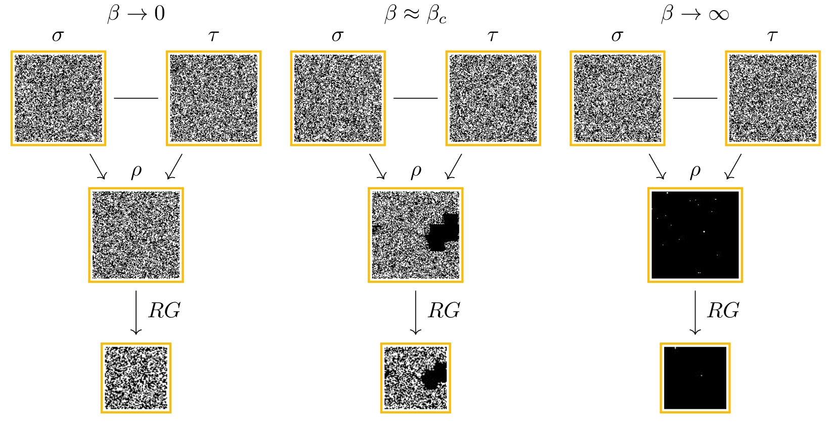
Figure 1: Illustrative examples of the renormalization group implementation based on the mapping of two replicas $\sigma$, $\tau$ to an overlap configuration $\rho$. The spin glass phase transition of the three-dimensional Edwards-Anderson model is mapped to a system with overlap degrees of freedom which manifests critical behavior that resembles ferromagnetism. The emergence of the spin glass correlation length can then be explicitly observed in the overlap configuration based on the creation of clusters. Renormalization group transformations, using the majority rule, are directly implemented on the overlap degrees of freedom. The $\beta\rightarrow\infty$ illustration depicts the case where the overlap order parameter $q\approx-1$.

Furthermore, in this manuscript, we utilize the renormalization group to study the explicit symmetry breaking within the two-replica Hamiltonian of the three-dimensional Edwards-Anderson model. Specifically, we couple the overlap order parameter to a fictitious field and introduce it within the two-replica Hamiltonian to break explicitly its symmetry. We then construct mappings which relate the original and the renormalized fictitious fields, and extract the critical exponent associated with the divergence of the correlation length in relation to the field of the overlap order parameter. Finally, we conclude by discussing how overlap renormalization group transformations, which do not require a renormalization of the random couplings of a system, enable the extraction of multiple critical exponents in phase transitions which are fully characterized by overlap order parameters.

II Spin glasses and the overlap

We consider the case of the three-dimensional Edwards-Anderson model with three replicas $\sigma$, $\tau$, $\upsilon$ which comprise spins $s$, $t$, $u$, respectively. To simplify notation we will derive equations based on two replicas $\sigma$, $\tau$. For a specific inverse temperature $\beta$ the Hamiltonian of the system is defined as:

$$E_{\sigma,\tau}=E_{\sigma}+E_{\tau}=-\sum_{\langle ij\rangle}J_{ij}(s_{i}s_{j}+t_{i}t_{j}),$$ (1)

where $\langle ij\rangle$ denotes a nearest-neighbor interaction for spins $s,t=\pm 1$, and $J_{ij}$ are random couplings sampled as $J_{ij}=\pm 1$ with equal probability. The replicas experience the same realization of disorder $\{J_{ij}\}$.

The system defines a joint Boltzmann probability distribution $p_{\sigma_{i},\tau_{j}}$ for two configurations $\sigma_{i}$, $\tau_{j}$ at inverse temperature $\beta$:

$$p_{\sigma_{i},\tau_{j}}=\frac{\exp[-\beta(E_{\sigma_{i}}+E_{\tau_{j}})]}{\sum_{\sigma}\sum_{\tau}\exp[-\beta(E_{\sigma}+E_{\tau})]},$$ (2)

where $Z_{\sigma,\tau}=\sum_{\sigma}\sum_{\tau}\exp[-\beta(E_{\sigma}+E_{\tau})]$ is the partition function and the sums are over all possible configurations $\sigma$, $\tau$. We remark that $Z_{\sigma,\tau}=Z_{\sigma}Z_{\tau}=Z_{\sigma}^{2}=Z_{\tau}^{2}\equiv Z^{2}$ in terms of the equilibrium occupation probabilities. However we keep the partition functions separated as we aim to estimate them independently based on a finite size of samples which is obtained from Markov chain Monte Carlo simulations.

An important quantity which characterizes the phase transition of the three-dimensional Edwards-Anderson model is the overlap order parameter $q$ defined in terms of two replicas $\sigma$ and $\tau$:

$$q_{\sigma\tau}=\frac{1}{V}\sum_{i}s_{i}t_{i},$$ (3)

where $V=L^{3}$ is the volume of the system.

The overlap order parameter is bound between $[-1,1]$. When in the spin glass phase, the value $q=1$ corresponds to the case where the spins in each set $\{s_{i},t_{i}\}$ of the two replicas $\sigma$, $\tau$ have identical values. In constrast, the value $q=-1$ corresponds to the case where all the spins $\{s_{i},t_{i}\}$ in the two replicas have exactly different values. In addition one can define the overlap susceptibility $\chi_{q}$ as:

$$\chi_{q}=\beta V(\langle q^{2}\rangle-\langle q\rangle^{2})=\beta V\langle q^{2}\rangle,$$ (4)

where $\langle q\rangle=0$.

It is now possible to map the two-replica system, based on the Haake-Lewenstein-Wilkens perspective, into a single system which comprises overlap degrees of freedom. Specifically, given two replicas $\sigma$, $\tau$ with spins $s$, $t$ and lattice size $L$ in each dimension we define a configuration $\rho$ with degrees of freedom $\varrho_{i}=s_{i}t_{i}$ and lattice size $\mathcal{L}=L$. This mapping defines an effective Hamiltonian $E^{\textrm{eff}}$, partition function $Z^{\textrm{eff}}$, and Boltzmann probability distribution $p^{\textrm{eff}}_{\rho_{i}}$ for the three-dimensional Edwards-Anderson model. The effective probability distribution $p^{\textrm{eff}}_{\rho_{i}}$, for a specific realization of disorder $\{J_{ij}\}$, has the form [16]:

$$p^{\textrm{eff}}_{\rho_{i}}[\{J_{ij}\}]=\frac{\exp\big{[}-\beta E^{\textrm{eff}}_{\rho_{i},\{J_{ij}\}}\big{]}}{Z^{\textrm{eff}}_{\rho}[\{J_{ij}\}]}=\sum_{\{s\}}\frac{\exp\big{[}\beta\sum_{\langle ij\rangle}J_{ij}(1+\varrho_{i}\varrho_{j})s_{i}s_{j}\big{]}}{Z^{2}[\{J_{ij}\}]}=2^{V}\frac{\exp\big{[}\beta\sum_{\langle ij\rangle}J_{ij}(1+\varrho_{i}\varrho_{j})\big{]}}{Z^{2}[\{J_{ij}\}]},$$ (5)

where the gauge transformation $J_{ij}=J_{ij}s_{i}s_{j}$ was used to obtain the last equation.

The first implication, which emerges from the aforementioned mapping, is that one can define the equivalent of a magnetization $m$ in the system with overlap degrees of freedom $\varrho$:

$$m=\frac{1}{V}\sum_{i}\varrho_{i}.$$ (6)

By recalling that $\varrho_{i}=s_{i}t_{i}$ we establish that the spin glass phase transition of the two-replica Hamiltonian, which is characterized by the overlap order parameter $q$, is now mapped to the phase transition of an effective system, characterized by the magnetization $m$, and with critical behavior which resembles ferromagnetism. Formally:

$$[\langle q\rangle]=\Big{[}\sum_{\sigma}\sum_{\tau}q_{\sigma\tau}p_{\sigma,\tau}\Big{]}=\Big{[}\sum_{\rho}m_{\rho}p_{\rho}^{\textrm{eff}}\Big{]}=\big{[}\langle m\rangle_{\textrm{eff}}\big{]},$$ (7)

where $\langle\rangle$ is the thermal average and $[]$ the average over realizations of disorder.

The mapping from the two-replica system to the effective system has certain implications in relation to the phase transition. Specifically, if we denote as $\xi(\sigma,\tau,\beta)$ and $\xi(\rho,\beta)$ the correlation lengths of the two-replica and the effective system respectively, then $\xi(\sigma,\tau,\beta)=\xi(\rho,\beta)\ \forall\ \beta\in(0,\infty)$. The two systems therefore have an identical correlation length for all inverse temperatures $\beta$. Since the correlation length diverges at the critical fixed point $\xi(\sigma,\tau,\beta_{c},L=\infty)=\xi(\rho,\beta_{c},\mathcal{L}=\infty)=\infty$ the aforementioned observation implies that the two systems have an identical fixed point $\beta_{c}$. In addition since observables of the two systems diverge according to the same correlation length $\xi$ this implies that the critical exponents of quantities associated with the overlap order parameter $q$ or, equivalently, with the magnetization $m$ are also identical for the two systems.

Monte Carlo renormalization group methods were first developed for the effective system by Wang and Swendsen [8]. One considers that the application of a renormalization group transformation is established on the effective probability distribution $p^{\textrm{eff}}$ to obtain a renormalized probability distribution $p^{{}^{\prime}\textrm{eff}}$ as:

$$p^{{}^{\prime}\textrm{eff}}_{\rho^{\prime}}=\sum_{\rho}T(\rho^{\prime},\rho)p^{\textrm{eff}}_{\rho},$$ (8)

where $T(\rho^{\prime},\rho)$ corresponds to the majority rule. Since $T(\rho^{\prime},\rho)$ has no explicit dependence on the random couplings the renormalization group transformation can be interchanged with the averaging over the realizations of disorder. The approach, including the application of renormalization group transformations on the system with overlap degrees of freedom is illustrated in Fig. 1.

We remark that, while it is of interest to introduce, within a renormalization group setting, correlation functions which have, for instance, the form of neighbor interactions $\varrho_{i}\varrho_{j}$ between the overlap degrees of freedom $\varrho$, we will not pursue this direction here. Instead, we will focus solely on quantities derived from the overlap order parameter $q$. These remain, probabilistically, observables of the original system and are therefore Boltzmann-distributed based on the original probability distribution of Eq. (2). We will then incorporate reweighting techniques within the computational renormalization group method to determine the critical fixed point and to extract four critical exponents.

III Parallel Tempering and Multi-histogram Reweighting

While one can, in principle, simulate directly the three-dimensional Edwards-Anderson model using a conventional Markov chain Monte Carlo simulation with the Metropolis algorithm, such computations can be prohibitively long due to issues pertinent to the thermalization of the Markov chain and the critical slowing down effect. To alleviate simulational problems, we utilize the parallel tempering technique.

We consider a set of inverse temperatures $\{\beta_{0},\beta_{1},\ldots,\beta_{m}\}$, with $\beta_{0}<\beta_{1}<\beta_{m}$. Specifically, we consider $m=19$ and $\beta_{0}=0.55$, $\beta_{m}=1.15$ where the set of inverse temperatures extends to the spin glass phase. In addition we impose the constraint that two adjacent inverse temperatures are sufficiently close in parameter space: this implies that there exists an overlap between the energy histograms for systems simulated at the two inverse temperatures.

We implement the parallel tempering technique by attempting an exchange of configurations for two simulated replicas at adjacent inverse temperatures. Specifically, if we consider two replicas at inverse temperatures $\beta_{0}$ and $\beta_{1}$ which have an energy difference of $\Delta E=E_{1}-E_{0}$, then an exchange of configurations is accepted based on the acceptance probability $\mathcal{A}$:

$$\mathcal{A}=\begin{cases}\exp\big{[}-(\beta_{0}-\beta_{1})\Delta E\big{]}&\text{if}\ \Delta E>0\\ 1&\text{otherwise}.\end{cases}$$ (9)

We are additionally interested in a complementary method, namely the multi-histogram reweighting technique. We aim to utilize the multiple histogram method to reweight observables of the renormalized systems under the probability distributions of the original systems. To the best of our knowledge, while reweighting has been utilized in disordered systems [30], this manuscript documents the first use of the multiple histogram method within a Monte Carlo renormalization group calculation of a disordered system. Detailed derivations for the multiple histogram method can be found, for instance, in Ref. [31].

To implement the multi-histogram reweighting technique for the replica $\sigma$ we optimize the partition function $Z_{\sigma,l}$ for each inverse temperature which belongs in the set $\{\beta_{0},\beta_{1},\ldots,\beta_{m}\}$ via:

$$Z_{\sigma,l}=\sum_{i,x}\frac{1}{\sum_{j}n_{j}Z_{\sigma,j}^{-1}\exp[(\beta_{l}-\beta_{j})E_{ix}]},$$ (10)

where the sum is over configurations $x$ which are sampled at simulation $i$ and have energy $E_{ix}$, $j$ is a sum over all simulations at inverse temperatures of the set $\{\beta_{0},\beta_{1},\ldots,\beta_{m}\}$ and $n_{j}$ is the number of configurations sampled at simulation $j$. After convergence is achieved, we estimate the partition function $Z_{\sigma}(\beta)$ for every inverse temperature $\beta$ in the continuous range $\beta\in[\beta_{0},\beta_{m}]$ via:

$$Z_{\sigma}(\beta)=\sum_{i,x}\frac{1}{\sum_{j}n_{j}Z_{\sigma,j}^{-1}\exp[(\beta-\beta_{j})E_{ix}]}.$$ (11)

Figure 2: The probability density function for the overlap order parameters $q_{\sigma\tau}$, $q_{\tau\upsilon}$, $q_{\sigma\upsilon}$ of three replicas $\sigma$, $\tau$, $\upsilon$ at inverse temperature $\beta=0.95$ and lattice size $L=16$ in each dimension. An initial number of configurations is discarded due to the thermalization of the Markov chain and the results are obtained based on subsequent measurements.

We complete the above process for the partition functions of both replicas $Z_{\sigma}$ and $Z_{\tau}$. For a given realization of disorder $J_{ij}$ the expectation value of any arbitrary observable $O$ defined on the two-replica Hamiltonian, can then be estimated via:

$$\langle O\rangle_{\beta}=\frac{1}{Z_{\sigma}(\beta)Z_{\tau}(\beta)}\sum_{i,x,y}\frac{O_{ixy}}{\sum_{j}n_{j}Z_{\sigma,j}^{-1}Z_{\tau,j}^{-1}\exp[-(\beta-\beta_{j})(E_{ix}+E_{iy})]},$$ (12)

where the sum is over configurations $x$, $y$ of replicas $\sigma$, $\tau$. We emphasize that the above equation can be additionally utilized to reweight observables $O^{\prime}$ of renormalized systems under the original probability distribution by substituting every occurence of $O$ with $O^{\prime}$. We consider an averaging over $25$ and $50$ realizations of disorder for systems with lattice sizes $L=16$ and $L=8$ in each dimension, respectively.

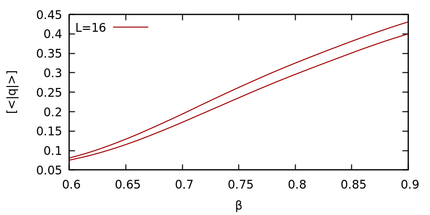
Figure 3: Expectation of the absolute value of the overlap order parameter $q$ calculated under a thermal $\langle\rangle$ and disorder $[]$ average versus the inverse temperature $\beta$. The results are obtained using parallel tempering and multi-histogram reweighting on a two-replica Hamiltonian. The space bounded by the lines corresponds to the statistical uncertainty.

In this manuscript we consider three replicas and thus we are able to calculate three values $q_{\sigma\tau}$, $q_{\tau\upsilon}$, $q_{\sigma\upsilon}$ of the overlap order parameter. In fact, we utilize these separate calculations, obtained via parallel tempering, to establish that the ensemble has successfully thermalized. The probability density function for $q_{\sigma\tau}$, $q_{\tau\upsilon}$, $q_{\sigma\upsilon}$ of a system at inverse temperature $\beta=0.95$ with lattice size $L=16$ and one realization of disorder is depicted in Fig. 2. We observe that the distribution is symmetric and in agreement for the three calculations, thus indicating that the system has successfully reached thermal equilibrium.

Having established a criterion for thermal equilibium we now utilize multi-histogram reweighting to interpolate the overlap order parameter in the range of $\beta\in[\beta_{0},\beta_{m}]$. Results within the critical region are depicted in Fig. 3. We emphasize that the use of multi-histogram reweighting simplifies considerably the renormalization group implementation as it provides results in the entire critical region and is essential to the computational approach discussed here.

IV Overlap renormalization group transformations

IV.1 The renormalization group

We are now able to implement a renormalization group transformation. which transforms the degrees of freedom defined by the overlap of the two replicas, for the three-dimensional Edwards-Anderson model. We recall that, given two replicas $\sigma$, $\tau$, we define a new lattice $\mathcal{L}$ where each site $i$ has the value $\varrho_{i}=s_{i}t_{i}$. Based on a rescaling factor of $b=2$ we then separate the lattice into blocks of size $b$ in each dimension and select the rescaled degree of freedom by applying the majority rule on the spins $\varrho$ within each block. When the number of positive and negative spins is equal we select randomly the rescaled degree of freedom.

Given an original system with overlap degrees of freedom and lattice size $\mathcal{L}$ or, equivalently, two replicas of lattice size $L$ in each dimension, we obtain via the renormalization group a rescaled system with lattice size $\mathcal{L}^{\prime}$:

$$\mathcal{L}^{\prime}=\frac{\mathcal{L}}{b}.$$ (13)

The spin glass correlation length $\xi$ of the original system is therefore transformed, in terms of lattice units, as:

$$\xi^{\prime}=\frac{\xi}{b}.$$ (14)

We remark that since the correlation length is a quantity which arises dynamically as we approach the critical fixed point, and the original and the renormalized systems are described by different correlation lengths $\xi$ and $\xi^{\prime}$ then this implies that the two systems have a different distance from the critical fixed point. Consequently, the two systems are described by different inverse temperatures $\beta$ and $\beta^{\prime}$ or, equivalently, by a different set of coupling constants.

IV.2 The fixed point and the exponents $\gamma/\nu$, $\kappa_{q}/\nu$

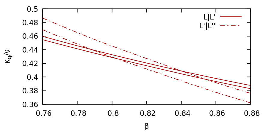
Figure 4: The critical exponent $\kappa_{q}/\nu$ versus the inverse temperature $\beta$. The space bounded by the lines corresponds to the statistical uncertainty.

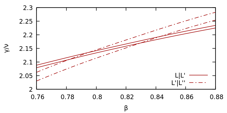
Figure 5: The critical exponent $\gamma/\nu$ versus the inverse temperature $\beta$. The space bounded by the lines corresponds to the statistical uncertainty.

We are now able to conduct a renormalization group study of the three-dimensional Edwards-Anderson model based on transformations applied on the degrees of freedom $\varrho$ defined by the overlap of two replicas. This is achieved by utilizing exclusively quantities derived from the overlap order parameter $q$, thus avoiding the need to undergo a renormalization of the random couplings of the system. We will calculate the critical fixed point and two critical exponents via a direct computational implementation of the Kadanoff scaling picture.

As an initial step we are interested in locating the critical fixed point which describes the finite-temperature spin glass transition of the system at a critical $\beta_{c}$. We define the reduced coupling constants $t$ and $t^{\prime}$ which measure the distance from the critical fixed point for an original and a renormalized system:

$$t=\frac{\beta_{c}-\beta}{\beta_{c}},\ t^{\prime}=\frac{\beta_{c}-\beta^{\prime}}{\beta_{c}},$$ (15)

We now define a critical exponent $\kappa_{q}$ which governs the divergence of the overlap order parameters $q$, $q^{\prime}$ of the original and the renormalized systems:

$$q\sim|t|^{\kappa_{q}},\ q^{\prime}\sim|t^{\prime}|^{\kappa_{q}}.$$ (16)

We remark that while the exponent coupled to the order parameter is often denoted as $\beta$, we utilize $\kappa_{q}$ to avoid confusion with the inverse temperature $\beta$. The above equations can be equivalently expressed in terms of the spin glass correlation lengths $\xi$, $\xi^{\prime}$ as:

$$q\sim\xi^{-\kappa_{q}/\nu},\ q^{\prime}\sim\xi^{\prime-\kappa_{q}/\nu},$$ (17)

where $\nu$ is the correlation length exponent. By dividing the above equations and taking the natural logarithm we arrive at the expression:

$$\frac{\kappa_{q}}{\nu}=\frac{\log\frac{q^{\prime}}{q}}{\log b}.$$ (18)

Following an analogous process we are able to calculate the exponent $\gamma$ of the overlap susceptibility $\chi_{q}$ via:

$$\frac{\gamma}{\nu}=-\frac{\log\frac{\chi_{q}^{\prime}}{\chi_{q}}}{\log b}.$$ (19)

We remark that since the correlation length diverges at the critical point $\xi(\beta_{c})=\xi^{\prime}(\beta_{c})=\infty$, one anticipates that all intensive observables $O$, $O^{\prime}$ of an original and a renormalized system intersect $O(\beta_{c})=O^{\prime}(\beta_{c})$. Nevertheless, while this observation is mathematically valid, in practical implementations such intersections are subject to finite size-effects and are not always observed. However, there exists another approach to determine the fixed point even under the presence of finite-size effects: one can directly search for an intersection between the exponents themselves [32].

Based on the above observation, we utilize multi-histogram reweighting to obtain calculations of effective critical exponents $\kappa_{q}/\nu$, $\gamma/\nu$ in the continuous range $\beta\in[\beta_{0},\beta_{m}]$. This simplifies significantly the computational calculations since it is not necessary to conduct additional simulations. The results, obtained by two iterative renormalization group applications on a system with lattice size $\mathcal{L}=16$ to produce two renormalized systems of lattice sizes $\mathcal{L}_{16}^{\prime}=8$ and $\mathcal{L}_{16}^{\prime\prime}=4$ in each dimension, are depicted in Figs. 4 and 5. We observe an intersection in parameter space for both calculations of the critical exponents. Consequently we obtain two estimates of the fixed point $\beta_{c}=0.814(32)$, $\beta_{c}=0.825(28)$ and the critical exponents $\gamma/\nu=2.17(4)$, $\kappa_{q}/\nu=0.41(2)$. For the calculation pertinent to the exponent $\kappa_{q}$ we utilize the absolute value of the overlap order parameter $|q|$.

We remark that, in the previous renormalization group approach, calculations are conducted based on quantities derived from the overlap order parameter, which can be calculated on original and renormalized configurations without knowledge of the random couplings. In addition, renormalized observables $O^{\prime}$ are reweighted under the original probability distribution and, therefore, under the original random couplings $\{J_{ij}\}$, which are known. In the next subsections, we will further improve on the previous calculations of the critical exponents by linearizing the renormalization group transformation.

IV.3 Inverse mappings and the exponent $\nu$

We will now utilize a different approach, namely the Wilson two-lattice matching Monte Carlo renormalization group. The method concerns the comparison of an original and a renormalized system of identical lattice size $\mathcal{L}=\mathcal{L}^{\prime}$. These two systems are described by different realizations of disorder $\{J_{ij}\}\neq\{J_{ij}^{\prime}\}$. Consequently the renormalization group method to be discussed below is affected more strongly by systematic errors pertinent to the averaging over a small number of disorder realizations but is affected less by systematic errors pertinent to finite-size effects.

To describe the method we consider again an original system of lattice size $\mathcal{L}=16$ to which we apply one renormalization group transformation to produce a renormalized system of lattice size $\mathcal{L}^{\prime}_{16}=8$. We now compare observables of the renormalized system $\mathcal{L}^{\prime}_{16}=8$ against observables of an original system $\mathcal{L}$ with $\mathcal{L}=\mathcal{L}^{\prime}_{16}=8$. By applying another renormalization group transformation on both systems we additionally conduct calculations for systems with $\mathcal{L}^{\prime}_{8}=\mathcal{L}^{\prime\prime}_{16}=4$. The benefit of the discussed renormalization group method is that by comparing two systems of identical lattice size one partially eliminates finite-size effects, and thus accurate calculations can be obtained on trivially small lattice sizes.

Figure 6: Expectation of the absolute value of the overlap order parameter, calculated with multi-histogram reweighting under thermal and disorder averaging, for an original and a renormalized system of identical lattice size $L=L_{16}^{\prime}=8$. The space bounded by the lines corresponds to the statistical uncertainty.

Figure 7: Expectation of the absolute value of the overlap order parameter, calculated with multi-histogram reweighting under thermal and disorder averaging, for two renormalized systems of identical lattice size $L_{8}^{\prime}=L_{16}^{\prime\prime}=4$. The space bounded by the lines corresponds to the statistical uncertainty.

We now utilize multi-histogram reweighting to obtain the absolute value of the overlap order parameter for systems with identical lattice size. The results are depicted in Figs. 6 and 7. Under the reduction of finite-size effects we are now able to observe an intersection of observables at the critical fixed point. Based on the discussed renormalization group approach, we obtain an estimate of the critical inverse temperature $\beta_{c}=0.751(47)$. This is comparable with related renormalization group implementations [8].

We additionally observe that the expected renormalization group flows have emerged. Specifically, for $\beta>\beta_{c}$ the overlap order parameter has values $|q^{\prime}|>|q|$ since the system has been driven deeper to the spin glass phase due to the reduction of the correlation length. In an analogous manner, for $\beta<\beta_{c}$ the renormalized system has been driven towards the zero inverse temperature, and thus $|q^{\prime}|<|q|$.

Having established that the renormalization group method produces the anticipated behaviour, it is now possible to determine the renormalized coupling parameters. Specifically, we are interested in extracting a function which is able to relate, for instance, the original and the renormalized inverse temperatures $\beta$, $\beta^{\prime}$. This can be achieved via the inverse mapping:

$$\beta^{\prime}=O^{-1}(O^{\prime}(\beta)).$$ (20)

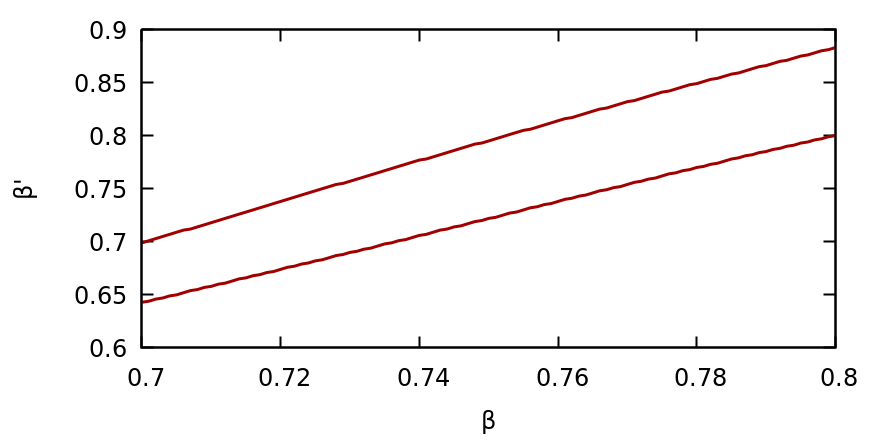
Figure 8: Renormalized inverse temperature $\beta^{\prime}$ versus original inverse temperature $\beta$. The space bounded by the lines corresponds to the statistical uncertainty.

Figure 9: Disorder-averaged renormalized inverse temperature $\beta^{\prime}$ versus disorder-averaged original inverse temperature $\beta$. The space bounded by the lines corresponds to the statistical uncertainty.

We can now utilize these mappings to extract the correlation length exponent $\nu$. Specifically, the divergence of the correlation lengths $\xi$, $\xi^{\prime}$ in terms of the reduced inverse temperatures $t$, $t^{\prime}$ is given by:

$$\xi\sim|t|^{-\nu},\ \xi^{\prime}\sim|t^{\prime}|^{-\nu}.$$ (21)

By dividing the two expressions, linearizing the transformation with a Taylor expansion [33], taking the natural logarithm, and considering one renormalization group application, we obtain the following relation which is valid in the vicinity of the critical point $\beta_{c}$:

$$\nu=\frac{\log b}{\log\frac{d\beta^{\prime}}{d\beta}}.$$ (22)

Based on the above expression, we are then able to calculate the correlation length exponent numerically.

Due to the nature of disordered systems and, specifically, the averaging over disorder there exist two distinct approaches that can be utilized to calculate the correlation length exponent: these produce different results. In the former approach we first conduct the thermal and disorder averaging to obtain $[\langle q^{\prime}\rangle]$, $[\langle q\rangle]$ and then construct the inverse mappings:

$$\beta^{\prime}=[\langle q\rangle]^{-1}([\langle q^{\prime}\rangle](\beta)).$$ (23)

By following this procedure, the results of which are depicted in Fig. 8, we obtain a calculation of the correlation length exponent as $\nu=1.24(4)$.

The second approach concerns the construction of mappings between $\beta^{\prime}$ and $\beta$ for individual realizations of disorder as:

$$\beta^{\prime}_{\{J_{ij}^{\prime}\}}=\langle q_{\{J_{ij}\}}\rangle^{-1}(\langle q_{\{J_{ij}^{\prime}\}}^{\prime}\rangle(\beta_{\{J_{ij}\}})).$$ (24)

In contrast to the previous approach, we will now construct disorder-averaged mappings. Specifically, since we consider $25$ and $50$ realizations of disorder for the systems with lattice sizes $\mathcal{L}^{\prime}_{16}=8$ and $\mathcal{L}=8$ we obtain $1250$ sets of mappings $\beta_{\{J_{ij}\}}$ to $\beta^{\prime}_{\{J_{ij}^{\prime}\}}$ from which we calculate the disorder-averaged mappings $[\beta]$ to $[\beta^{\prime}]$ that are depicted in Fig. 9. Following this procedure, we calculate the correlation length exponent as $\nu=2.60(7)$.

We observe a discrepancy in the calculation of the exponent $\nu$ depending on how the averaging over disorder is conducted. This discrepancy could be of numerical nature: the method is dependent on the construction of mappings by establishing an equivalence of observables between two systems over a large region of parameter space which extends above and below the fixed point. It is of interest to explore if this discrepancy would vanish in larger lattices and under an averaging over a larger number of realizations of disorder.

IV.4 Explicit symmetry breaking and the exponent $\theta_{\epsilon}$

We have so far utilized quantities derived from the overlap order parameter $q$ to obtain independent calculations of the critical exponents $\nu$, $\gamma/\nu$ and $\kappa_{q}/\nu$. This is achieved by studying the corresponding phase transition based on the divergence of the correlation length $\xi$ in relation to the inverse temperature $\beta$.

We proceed to study a different setting with the Wilson two-lattice matching renormalization group. Specifically, we are now interested in coupling the overlap order parameter $q$ to a fictitious field $\epsilon$ and introducing it within the two-replica Hamiltonian of the three-dimensional Edwards-Anderson to induce explicit symmetry breaking. We will then construct mappings which relate the original and the renormalized fields $\epsilon$, $\epsilon^{\prime}$ and we will extract an additional exponent, namely the exponent $\theta_{\epsilon}$ which, in this case, governs the divergence of the spin glass correlation length $\xi$ in relation to the fictitious field $\epsilon$.

To initiate our study we modify the Hamiltonian of Eq. (1) by introducing the overlap order parameter $q$ coupled to a fictitious field $\epsilon$. For simplicity, we will subsequently call $\epsilon$ the replica field. The modified Hamiltonian is:

$$E_{\sigma,\tau}^{\prime}=E_{\sigma}+E_{\tau}-\epsilon Vq_{\sigma\tau},$$ (25)

and defines a modified Boltzmann probability distribution:

$$p_{\sigma_{i},\tau_{j}}^{\prime}=\frac{\exp[-\beta(E_{\sigma_{i}}+E_{\tau_{j}}-\epsilon Vq_{\sigma_{i}\tau_{j}})]}{\sum_{\sigma}\sum_{\tau}\exp[-\beta(E_{\sigma}+E_{\tau}-\epsilon Vq_{\sigma\tau})]}.$$ (26)

We remark that, in principle, the above probability distribution could be directly sampled with Markov chain Monte Carlo simulations. Nevertheless we anticipate that, due to the introduced term, such simulations might be complicated. To avoid sampling we instead utilize reweighting to obtain expectation values pertinent to the above probability distribution based on the original configurations sampled with the probability distribution of Eq. (2). Specifically, we consider, for a given realization of disorder, the expectation value of an arbitrary observable $O$ calculated under the two-replica probability distribution $p_{\sigma_{i},\tau_{j}}^{\prime}$:

$$\langle O\rangle=\frac{\sum_{\sigma}\sum_{\tau}O_{\sigma\tau}\exp[-\beta(E_{\sigma}+E_{\tau}-\epsilon Vq_{\sigma\tau})]}{\sum_{\sigma}\sum_{\tau}\exp[-\beta(E_{\sigma}+E_{\tau}-\epsilon Vq_{\sigma\tau})]},$$ (27)

where the sums are over all configurations. We aim to approximate the above expectation value based on a numerical estimator with a set of sampling probabilities $\tilde{p}_{\sigma_{i},\tau_{j}}$:

$$\langle O\rangle=\frac{\sum_{i=1}^{N_{\sigma}}\sum_{j=1}^{N_{\tau}}O_{\sigma_{i}\tau_{j}}\tilde{p}_{\sigma_{i},\tau_{j}}^{-1}\exp[-\beta(E_{\sigma_{i}}+E_{\tau_{j}}-\epsilon Vq_{\sigma_{i}\tau_{j}})]}{\sum_{i=1}^{N_{\sigma}}\sum_{j=1}^{N_{\tau}}\tilde{p}_{\sigma_{i},\tau_{j}}^{-1}\exp[-\beta(E_{\sigma_{i}}+E_{\tau_{j}}-\epsilon Vq_{\sigma_{i}\tau_{j}})]}.$$ (28)

where $N_{\sigma}$ and $N_{\tau}$ correspond to the number of configurations sampled for each replica $\sigma$, $\tau$.

Since we will sample $p_{\sigma,\tau}^{\prime}$ with the probability distribution of the original system we set $\tilde{p}_{\sigma,\tau}=p_{\sigma,\tau}$ and we obtain:

$$\langle O\rangle=\frac{\sum_{i=1}^{N_{\sigma}}\sum_{j=1}^{N_{\tau}}O_{\sigma_{i}\tau_{j}}\exp[\beta\epsilon Vq_{\sigma_{i}\tau_{j}})]}{\sum_{i=1}^{N_{\sigma}}\sum_{j=1}^{N_{\tau}}\exp[\beta\epsilon Vq_{\sigma_{i}\tau_{j}})]}.$$ (29)

Using the above reweighting expression, which is agnostic to the original Hamiltonian [26], we are able to calculate expectation values of observables $O_{\sigma\tau}$ at inverse temperature $\beta$ for a nonzero replica field $\epsilon$. We achieve this by utilizing instead the original configurations at the same inverse temperature $\beta$ which have been simulated for a zero value of the replica field. We emphasize that, by substituting every occurence of $O$ with $O^{\prime}$ we are additionally able to obtain expectation values for any renormalized observable $O^{\prime}$.

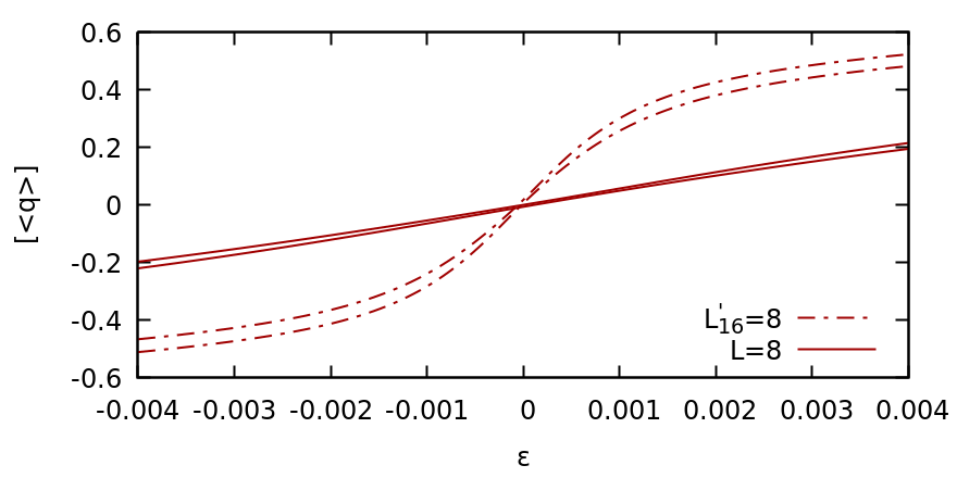
Figure 10: Expectation of the overlap order parameter $q$ versus the replica field $\epsilon$ for an original and a renormalized system. The space bounded by the lines corresponds to the statistical uncertainty.

The expectation value of the overlap order parameter $q_{\sigma\tau}$ for an original and a renormalized system of identical lattice size is depicted for nonzero values of the replica field $\epsilon$ in Fig. 10. We observe that the overlap order parameter $q$ is driven towards positive or negative values when the replica field $\epsilon$ is positive or negative, respectively. This behavior is attributed to explicit symmetry breaking. Consequently, for positive or negative values of $\epsilon$ the spins of the two replicas tend to identical or exactly different values, respectively.

We are now interested in utilizing the results depicted in Fig. 10 to extract the critical exponent associated with the divergence of the spin glass correlation length $\xi$ in relation to the replica field $\epsilon$. To achieve this, we first construct inverse mappings which relate the original and the renormalized replica fields $\epsilon$, $\epsilon^{\prime}$ via:

$$\epsilon^{\prime}=O^{-1}(O^{\prime}(\epsilon)).$$ (30)

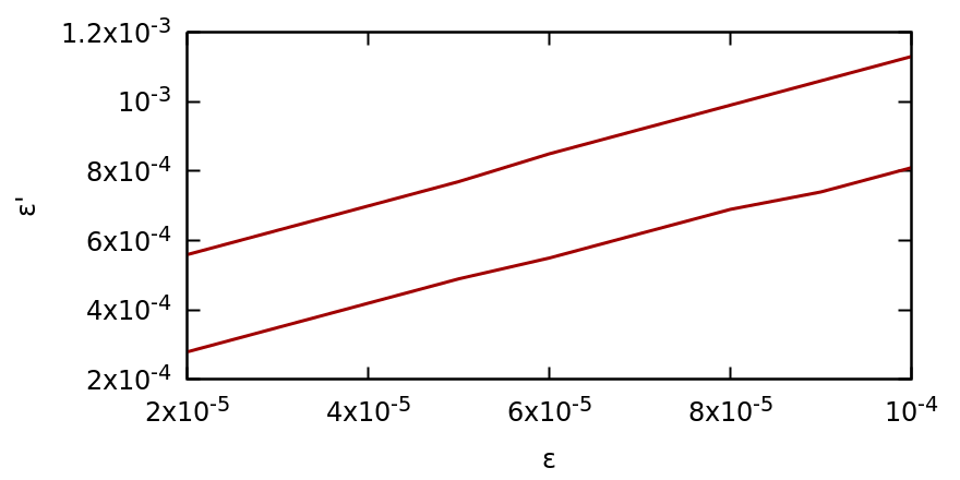
Figure 11: Renormalized replica field $\epsilon^{\prime}$ versus original replica field $\epsilon$. The space bounded by the lines corresponds to the statistical uncertainty.

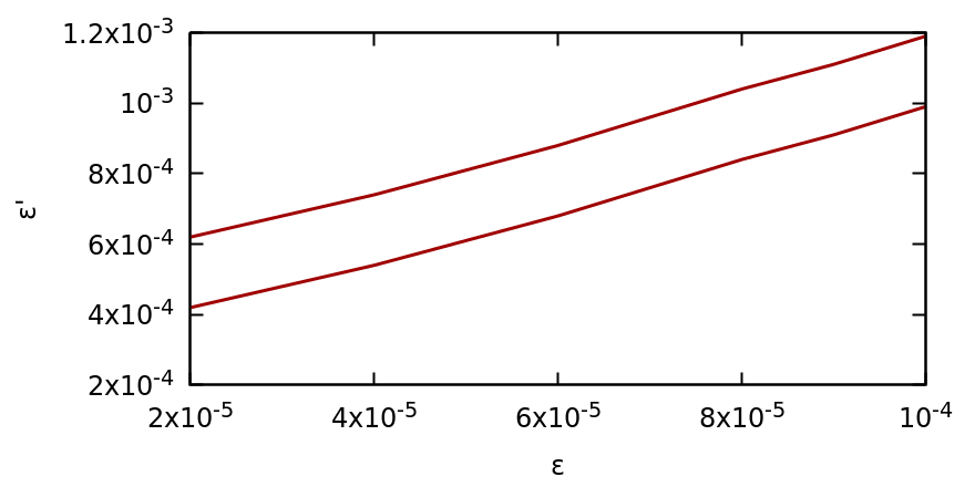
Figure 12: Disorder-averaged renormalized replica field $\epsilon^{\prime}$ versus disorder-averaged original replica field $\epsilon$. The space bounded by the lines corresponds to the statistical uncertainty.

We now define an exponent $\theta_{\epsilon}$ which governs the divergence of the spin glass correlation length in terms of the replica fields $\epsilon$, $\epsilon^{\prime}$ as:

$$\xi\sim|\epsilon|^{-\theta_{\epsilon}},\ \xi^{\prime}\sim|\epsilon^{\prime}|^{-\theta_{\epsilon}}.$$ (31)

The numerical calculation of the exponent $\theta$ is therefore achieved via:

$$\theta_{\epsilon}=\frac{\ln b}{\ln\frac{d\epsilon^{\prime}}{d\epsilon}}.$$ (32)

The above expression is valid in the vicinity of the critical fixed point $\beta_{c}$ and while $\epsilon\rightarrow 0$.

Following the same approach as for the exponent $\nu$ we conduct two calculations of $\theta_{\epsilon}$: the former is conducted by constructing mappings after the thermal and disorder averaging of the observables $[\langle q^{\prime}\rangle]$, $[\langle q\rangle]$ and the latter by constructing mappings for each individual realization of $\{J_{ij}\}$, $\{J_{ij}^{\prime}\}$ which are then averaged over disorder to obtain $[\epsilon^{\prime}]$, $[\epsilon]$. The mappings for the former and the latter approach are depicted in Figs. 11 and 12. We obtain a calculation of $\theta_{\epsilon}=0.370(9)$ and $\theta_{\epsilon}=0.377(7)$, respectively.

We observe, in constrast to the calculation of the exponent $\nu$, that there exists no large discrepancy in the calculation of the exponent $\theta_{\epsilon}$ with the two approaches. This is anticipated as, in contrast to the inverse temperature where the mappings are constructed in an extended region of parameter space above and below the fixed point $\beta_{c}$, in the case of $\theta_{\epsilon}$ the mappings are constructed in a small region of parameter space of range $10^{-4}$ as $\epsilon\rightarrow 0^{+}$.

IV.5 Improving the calculations of $\gamma/\nu$, $\kappa_{q}/\nu$

Having obtained a critical fixed point from the Wilson two-lattice matching Monte Carlo renormalization group method we can now conduct another set of calculations for the exponents $\gamma/\nu$, $\kappa_{q}/\nu$. The previous calculations of $\gamma/\nu$, $\kappa_{q}/\nu$ served only as a means to obtain an initial estimate of the fixed point without assuming any prior knowledge about the phase transition of the system. In fact, these calculations utilize equations which are strictly correct for the infinite-volume system and the estimates for these exponents should not be regarded as high-precision measurements.

We will improve the accuracy of the previous calculations and render the equations suitable for finite systems by linearizing the renormalization group transformation. In contrast to the previous calculations of $\gamma/\nu$, $\kappa_{q}/\nu$, which are conducted at a specific point in parameter space, we will now conduct the calculations via the use of finite differences. The benefit of considering finite differences is that one obtains robust calculations of critical quantities even if the system does not reside exactly at the critical fixed point. Specifically, we utilize L’H$\mathrm{\hat{o}}$pital’s rule to obtain [27]:

$$\frac{\kappa_{q}}{\nu}=\frac{\log\frac{dq^{\prime}}{dq}}{\log b},$$ (33)

$$\frac{\gamma}{\nu}=-\frac{\log\frac{d\chi_{q}^{\prime}}{d\chi_{q}^{\prime}}}{\log b}.$$ (34)

We now proceed to conduct the calculation of the exponents in the critical region which corresponds to the fixed point that emerged from the two-lattice matching approach. Based on the values of the overlap order parameter, which are depicted in Figs. 3 and 6, we utilize systems with lattice sizes $\mathcal{L}^{\prime}\neq\mathcal{L}$ to obtain a calculation of $\kappa_{q}/\nu=0.32(2)$. The values of the overlap susceptibility for the two systems are depicted in Figs. 13 and 14. We obtain for the overlap susceptibility exponent $\gamma/\nu=2.26(4)$.

Figure 13: Expectation value of the overlap susceptibility $\chi_{q}$ versus the inverse temperature for lattice size $L=16$. The space bounded by the lines corresponds to the statistical uncertainty.

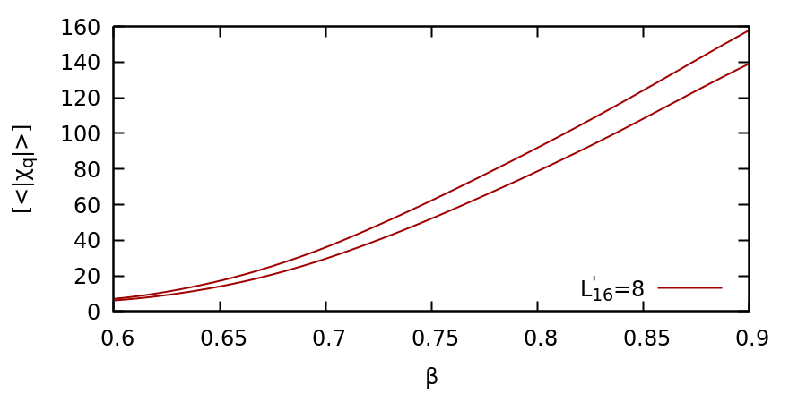
Figure 14: Expectation value of the overlap susceptibility $\chi_{q}$ versus the inverse temperature for lattice size $L^{\prime}_{16}=8$. The space bounded by the lines corresponds to the statistical uncertainty.

V Discussion

The results of this manuscript, obtained via the Wilson two-lattice matching renormalization group method or from a direct computational implementation of the Kadanoff scaling picture are summarized in Table 1. We find that calculations of the two critical exponents $\nu=1/{y_{t}}$ and $\theta_{\epsilon}=1/y_{h}$, which are obtained with the Wilson two-lattice matching method, are in agreement, within statistical errors, with Monte Carlo renormalization group calculations of the linearized matrix [8]. Based on the effective system, which comprises overlap degrees of freedom, it is conjectured within the Haake-Lewenstein-Wilkens [16, 34] perspective that the three-dimensional Edwards-Anderson model is characterized by a correlation length exponent $\nu$ which is two times the correlation length exponent of the conventional three-dimensional Ising model. The result of $\nu=1.24(4)$, obtained by first averaging over disorder and then constructing the mappings, supports this conjecture. Critical exponents for the three-dimensional Ising model have been calculated, for instance, with the conformal bootstrap method [35]. We remark that different renormalization group transformations produce different fixed points: these are not necessarily representative of physical values [21]. Nevertheless, the emergence of a critical fixed point supports, based on renormalization group arguments, the evidence for the presence of a finite-temperature spin glass transition for the three-dimensional Edwards-Anderson model.

Alternative theoretical methods which are commonly used to obtain critical exponents and the critical inverse temperature of systems that undergo phase transitions include finite-size scaling, nonequilibrium relaxation approaches and series expansions. These are generally conducted on the original Hamiltonian. Critical exponents can additionally be calculated via experiments [36]. Specifically, $\mathrm{Fe_{0.5}Mn_{0.5}TiO_{3}}$ is anticipated to manifest behavior similar to the three-dimensional Edwards-Anderson model with the spins aligned along the hexagonal c-axis. The experimental results are affected strongly by the choice of the critical temperature and are summarized in Ref. [37].

Historical values of critical quantities based on Refs. [38, 39, 40, 41, 42, 43, 44, 45, 46, 47, 48, 49, 50, 51, 52, 53, 54, 55, 56] are summarized in Ref. [57]. More recent results [58] include calculations conducted on the Janus dedicated computer [59]. We remark that, within errors, calculations of the correlation length exponent in these theoretical studies range from $\nu=1.1$ to $\nu=3.9$: this is not surprising given the difficulty in studying spin glasses. Nevertheless, the calculation of the correlation length exponent $\nu=2.60(7)$ obtained by first constructing the mappings between individual realizations of disorder and then averaging, is in agreement within statistical errors with the calculation by the Janus dedicated computer [59]. It might be interesting to comment on the fact, discussed in Ref. [57] that, even within the same finite-size scaling analysis, the method utilized to obtain the infinite-volume limit extrapolation can produce substantially different values, such as $\nu=2.39(5)$ or $\nu=1.49(6)$. An analogous discrepancy in the approach utilized to calculate the correlation length exponent with the renormalization group is additionally observed in the current manuscript.

We emphasize that, since four critical exponents have been calculated, it is possible to utilize scaling relations [31] to obtain multiple calculations of all exponents that describe the phase transition of the model. In fact, independent calculations of multiple critical exponents can additionally be utilized to verify if there exists a violation in scaling relations. For completeness, some scaling relations are:

$$\alpha=2-\nu d,$$ (35)

$$\frac{\kappa_{q}}{\nu}=d-\frac{1}{\theta_{\epsilon}},$$ (36)

$$\frac{\gamma}{\nu}=\frac{2}{\theta_{\epsilon}}-d,$$ (37)

$$\delta=\frac{1}{d\theta_{\epsilon}-1},$$ (38)

$$\eta=d+2-\frac{2}{\theta_{\epsilon}},$$ (39)

where $\alpha$ is the critical exponent which governs the singularity in the specific heat $c\sim|t|^{-\alpha}$, $\delta$ the exponent which governs the singularity of the overlap order parameter $q$ in terms of the replica field $\epsilon$, $q\sim\epsilon^{\frac{1}{\delta}}$, and $\eta$ the exponent defined from the two point correlation function $G$, $G(r,t)\sim 1/(r^{d-2+\eta})$. We have not assumed any form of correction or violation in the above equations.

Besides cross-verifying results with the four estimated critical exponents, it is of interest to utilize the estimations to calculate the critical exponent $\alpha$ of the specific heat. In general, to obtain a direct calculation of the exponent $\alpha$ within a renormalization group setting one would need to calculate the internal energy of the system and, consequently, one would need to renormalize the random couplings. Nevertheless, by utilizing the overlap order parameter $q$ to obtain an estimation of the correlation length exponent $\nu$ it is still possible to estimate $\alpha$, an exponent associated with an experimentally relevant quantity, without undergoing a renormalization of the random couplings. By utilizing the scaling relation we therefore obtain, based on the values of the correlation length exponent $\nu=1.24(4)$, $\nu=2.60(7)$, estimations of the specific heat exponent $\alpha=-1.72(12)$ and $\alpha=-5.80(21)$.

The results in this manuscript consider only statistical errors. Systematic errors that emerge in the calculations include the averaging over a finite number of realizations of disorder, the finite-size effects from considering small lattice sizes and the operators utilized to conduct the renormalization group calculation. More simulations on larger lattices are required.

	$\nu$	$\kappa_{q}/\nu$	$\gamma/\nu$	$\theta_{\epsilon}$
W	$1.24(4)|2.60(7)$	$0.32(2)$	$2.26(4)$	$0.370(9)|0.377(7)$
K	-	$0.41(2)$	$2.17(4)$	-

Table 1: Estimates of the critical exponents $\nu$, $\kappa_{q}/\nu$, $\gamma/\nu$, $\theta_{q}$ for the three-dimensional Edwards-Anderson model. We denote the exponent of the overlap order parameter as $\kappa_{q}$ to avoid confusion with the inverse temperature $\beta$. The calculations are conducted based on the Wilson two-lattice matching approach (W) or a direct computational implementation of the Kadanoff scaling picture (K).

VI Conclusions

By mapping the spin glass phase transition of the three dimensional Edwards-Anderson model to an effective system, which manifests critical behavior that resembles ferromagnetism, we have shown that the implementation of renormalization group transformations on the overlap degrees of freedom enables the determination of the critical fixed point and the calculation of four critical exponents. Furthermore, we have conducted a renormalization group study of the explicit symmetry-breaking of the system. Specifically, we constructed inverse mappings to extract the function which relates the original and the renormalized field that is coupled to the overlap order parameter.

In addition, we have utilized reweighting techniques for renormalized observables under the original probability distribution to study the spin glass phase transition. These enable high-precision calculations for Monte Carlo renormalization group methods. Specifically, when combined with parallel tempering, the multiple histogram method provides results in the entire critical region: it is therefore possible to determine the critical fixed point via an intersection of original and renormalized observables without requiring additional simulations. Reweighting techniques in Monte Carlo renormalization group methods additionally overcome the need to simulate a Hamiltonian, which includes the overlap order parameter, to induce explicit symmetry breaking in the original or renormalized system.

In summary, the utilization of renormalization group transformations on the overlap degrees of freedom enables the determination of the fixed point and the calculation of four critical exponents without the need to conduct a renormalization of the random couplings of the system. All other critical exponents can then be obtained via scaling relations. Consequently the discussed approach, enables studies of phase transitions that are fully characterized by overlap order parameters. It is therefore of interest to extend these techniques to other disordered systems, which also manifest glassy behavior.

References

- Kadanoff [1966] L. P. Kadanoff, Scaling laws for ising models near , Physics Physique Fizika 2, 263 (1966).
- Wilson [1971] K. G. Wilson, Renormalization group and critical phenomena. i. renormalization group and the kadanoff scaling picture, Phys. Rev. B 4, 3174 (1971).
- Wilson and Fisher [1972] K. G. Wilson and M. E. Fisher, Critical exponents in 3.99 dimensions, Phys. Rev. Lett. 28, 240 (1972).
- Wilson and Kogut [1974] K. G. Wilson and J. Kogut, The renormalization group and the expansion, Physics Reports 12, 75 (1974).
- Wilson [1975] K. G. Wilson, The renormalization group: Critical phenomena and the kondo problem, Rev. Mod. Phys. 47, 773 (1975).
- Mézard et al. [1987] M. Mézard, G. Parisi, and M. A. Virasoro, Spin Glass Theory and Beyond: An Introduction to the Replica Method and Its Applications (World Scientific, Singapore, 1987).
- Harris et al. [1976] A. B. Harris, T. C. Lubensky, and J.-H. Chen, Critical properties of spin-glasses, Phys. Rev. Lett. 36, 415 (1976).
- Wang and Swendsen [1988a] J.-S. Wang and R. H. Swendsen, Monte carlo renormalization-group study of ising spin glasses, Phys. Rev. B 37, 7745 (1988a).
- Angelini et al. [2013] M. C. Angelini, G. Parisi, and F. Ricci-Tersenghi, Ensemble renormalization group for disordered systems, Phys. Rev. B 87, 134201 (2013).
- Angelini and Biroli [2015] M. C. Angelini and G. Biroli, Spin glass in a field: A new zero-temperature fixed point in finite dimensions, Phys. Rev. Lett. 114, 095701 (2015).
- Angelini and Biroli [2017] M. C. Angelini and G. Biroli, Real space migdal–kadanoff renormalisation of glassy systems: Recent results and a critical assessment, Journal of Statistical Physics 167, 476 (2017).
- Parisi [1979] G. Parisi, Infinite number of order parameters for spin-glasses, Phys. Rev. Lett. 43, 1754 (1979).
- Parisi [1983] G. Parisi, Order parameter for spin-glasses, Phys. Rev. Lett. 50, 1946 (1983).
- Mézard et al. [1984] M. Mézard, G. Parisi, N. Sourlas, G. Toulouse, and M. Virasoro, Nature of the spin-glass phase, Phys. Rev. Lett. 52, 1156 (1984).
- Edwards and Anderson [1975] S. F. Edwards and P. W. Anderson, Theory of spin glasses, Journal of Physics F: Metal Physics 5, 965 (1975).
- Haake et al. [1985] F. Haake, M. Lewenstein, and M. Wilkens, Relation of random and competing nonrandom couplings for spin-glasses, Phys. Rev. Lett. 55, 2606 (1985).
- Lewenstein et al. [2022] M. Lewenstein, D. Cirauqui, M. Ángel García-March, G. G. i Corominas, P. Grzybowski, J. R. M. Saavedra, M. Wilkens, and J. Wehr, Haake–lewenstein–wilkens approach to spin-glasses revisited, Journal of Physics A: Mathematical and Theoretical 55, 454002 (2022).
- Biroli et al. [2018a] G. Biroli, C. Cammarota, G. Tarjus, and M. Tarzia, Random-field ising-like effective theory of the glass transition. i. mean-field models, Phys. Rev. B 98, 174205 (2018a).
- Biroli et al. [2018b] G. Biroli, C. Cammarota, G. Tarjus, and M. Tarzia, Random field ising-like effective theory of the glass transition. ii. finite-dimensional models, Phys. Rev. B 98, 174206 (2018b).
- Swendsen and Wang [1986] R. H. Swendsen and J.-S. Wang, Replica monte carlo simulation of spin-glasses, Phys. Rev. Lett. 57, 2607 (1986).
- Swendsen [1979] R. H. Swendsen, Monte carlo renormalization group, Phys. Rev. Lett. 42, 859 (1979).
- Wilson [1980] K. G. Wilson, in Recent Developments in Gauge Theories, edited by G. Hooft, C. Itzykson, A. Jaffe, H. Lehmann, P. K. Mitter, I. M. Singer, and R. Stora (Springer New York, New York, 1980).
- Pawley et al. [1984] G. S. Pawley, R. H. Swendsen, D. J. Wallace, and K. G. Wilson, Monte Carlo renormalization-group calculations of critical behavior in the simple-cubic Ising model, Phys. Rev. B 29, 4030 (1984).
- Hukushima and Nemoto [1996] K. Hukushima and K. Nemoto, Exchange monte carlo method and application to spin glass simulations, Journal of the Physical Society of Japan 65, 1604 (1996), https://doi.org/10.1143/JPSJ.65.1604 .
- Marinari and Parisi [1992] E. Marinari and G. Parisi, Simulated tempering: A new monte carlo scheme, Europhysics Letters 19, 451 (1992).
- Bachtis et al. [2021] D. Bachtis, G. Aarts, and B. Lucini, Adding machine learning within hamiltonians: Renormalization group transformations, symmetry breaking and restoration, Phys. Rev. Research 3, 013134 (2021).
- Bachtis et al. [2022] D. Bachtis, G. Aarts, F. Di Renzo, and B. Lucini, Inverse renormalization group in quantum field theory, Phys. Rev. Lett. 128, 081603 (2022).
- Bachtis [2022] D. Bachtis, Reducing finite-size effects in quantum field theories with the renormalization group 10.48550/arxiv.2205.08156 (2022).
- Ferrenberg and Swendsen [1989] A. M. Ferrenberg and R. H. Swendsen, Optimized monte carlo data analysis, Phys. Rev. Lett. 63, 1195 (1989).
- Janke [2003] W. Janke, Histograms and all that, in Computer Simulations of Surfaces and Interfaces, edited by B. Dünweg, D. P. Landau, and A. I. Milchev (Springer Netherlands, Dordrecht, 2003) pp. 137–157.
- Newman and Barkema [1999] M. E. J. Newman and G. T. Barkema, Monte Carlo methods in statistical physics (Clarendon Press, Oxford, 1999).
- Swendsen and Krinsky [1979] R. H. Swendsen and S. Krinsky, Monte carlo renormalization group and ising models with n¿ 2, Phys. Rev. Lett. 43, 177 (1979).
- Niemeijer and van Leeuwen [1976] T. Niemeijer and J. M. J. van Leeuwen, Phase Transitions and Critical Phenomena (Academic Press, 1976) edited by C. Domb and M. S. Green.
- Wang and Swendsen [1988b] J.-S. Wang and R. H. Swendsen, Monte carlo and high-temperature-expansion calculations of a spin-glass effective hamiltonian, Phys. Rev. B 38, 9086 (1988b).
- El-Showk et al. [2014] S. El-Showk, M. F. Paulos, D. Poland, S. Rychkov, D. Simmons-Duffin, and A. Vichi, Solving the 3d ising model with the conformal bootstrap ii. $$c$$-minimization and precise critical exponents, Journal of Statistical Physics 157, 869 (2014).
- Gunnarsson et al. [1991] K. Gunnarsson, P. Svedlindh, P. Nordblad, L. Lundgren, H. Aruga, and A. Ito, Static scaling in a short-range ising spin glass, Phys. Rev. B 43, 8199 (1991).
- Young [1998] A. Young, Spin Glasses and Random Fields, Directions in condensed matter physics (World Scientific, 1998).
- Ogielski and Morgenstern [1985] A. T. Ogielski and I. Morgenstern, Critical behavior of three-dimensional ising spin-glass model, Phys. Rev. Lett. 54, 928 (1985).
- Ogielski [1985] A. T. Ogielski, Dynamics of three-dimensional ising spin glasses in thermal equilibrium, Phys. Rev. B 32, 7384 (1985).
- McMillan [1985] W. L. McMillan, Domain-wall renormalization-group study of the three-dimensional random ising model at finite temperature, Phys. Rev. B 31, 340 (1985).
- Singh and Chakravarty [1986] R. R. P. Singh and S. Chakravarty, Critical behavior of an ising spin-glass, Phys. Rev. Lett. 57, 245 (1986).
- Bray and Moore [1985] A. J. Bray and M. A. Moore, Critical behavior of the three-dimensional ising spin glass, Phys. Rev. B 31, 631 (1985).
- Bhatt and Young [1985] R. N. Bhatt and A. P. Young, Search for a transition in the three-dimensional j ising spin-glass, Phys. Rev. Lett. 54, 924 (1985).
- Bhatt and Young [1988] R. N. Bhatt and A. P. Young, Numerical studies of ising spin glasses in two, three, and four dimensions, Phys. Rev. B 37, 5606 (1988).
- Kawashima and Young [1996] N. Kawashima and A. P. Young, Phase transition in the three-dimensional ising spin glass, Phys. Rev. B 53, R484 (1996).
- Bernardi et al. [1996] L. W. Bernardi, S. Prakash, and I. A. Campbell, Ordering temperatures and critical exponents in ising spin glasses, Phys. Rev. Lett. 77, 2798 (1996).
- Iñiguez et al. [1996] D. Iñiguez, G. Parisi, and J. J. Ruiz-Lorenzo, Simulation of three-dimensional ising spin glass model using three replicas: study of binder cumulants, Journal of Physics A: Mathematical and General 29, 4337 (1996).
- Berg and Janke [1998] B. A. Berg and W. Janke, Multioverlap simulations of the 3d edwards-anderson ising spin glass, Phys. Rev. Lett. 80, 4771 (1998).
- Marinari et al. [1998] E. Marinari, G. Parisi, and J. J. Ruiz-Lorenzo, Phase structure of the three-dimensional edwards-anderson spin glass, Phys. Rev. B 58, 14852 (1998).
- Palassini and Caracciolo [1999] M. Palassini and S. Caracciolo, Universal finite-size scaling functions in the 3d ising spin glass, Phys. Rev. Lett. 82, 5128 (1999).
- Mari and Campbell [1999] P. O. Mari and I. A. Campbell, Ising spin glasses: Corrections to finite size scaling, freezing temperatures, and critical exponents, Phys. Rev. E 59, 2653 (1999).
- Ballesteros et al. [2000] H. G. Ballesteros, A. Cruz, L. A. Fernández, V. Martín-Mayor, J. Pech, J. J. Ruiz-Lorenzo, A. Tarancón, P. Téllez, C. L. Ullod, and C. Ungil, Critical behavior of the three-dimensional ising spin glass, Phys. Rev. B 62, 14237 (2000).
- Mari and Campbell [2002] P. O. Mari and I. A. Campbell, Ordering temperature and critical exponents of the binomial ising spin glass in dimension 3, Phys. Rev. B 65, 184409 (2002).
- Nakamura et al. [2003] T. Nakamura, S. ichi Endoh, and T. Yamamoto, Weak universality of spin-glass transitions in three-dimensional ±j models, Journal of Physics A: Mathematical and General 36, 10895 (2003).
- Pleimling and Campbell [2005] M. Pleimling and I. A. Campbell, Dynamic critical behavior in ising spin glasses, Phys. Rev. B 72, 184429 (2005).
- Toldin et al. [2006] F. P. Toldin, A. Pelissetto, and E. Vicari, Critical behaviour of the random-anisotropy model in the strong-anisotropy limit, Journal of Statistical Mechanics: Theory and Experiment 2006, P06002 (2006).
- Katzgraber et al. [2006] H. G. Katzgraber, M. Körner, and A. P. Young, Universality in three-dimensional ising spin glasses: A monte carlo study, Phys. Rev. B 73, 224432 (2006).
- Hasenbusch et al. [2008] M. Hasenbusch, A. Pelissetto, and E. Vicari, Critical behavior of three-dimensional ising spin glass models, Phys. Rev. B 78, 214205 (2008).
- Baity-Jesi et al. [2013] M. Baity-Jesi, R. A. Baños, A. Cruz, L. A. Fernandez, J. M. Gil-Narvion, A. Gordillo-Guerrero, D. Iñiguez, A. Maiorano, F. Mantovani, E. Marinari, V. Martin-Mayor, J. Monforte-Garcia, A. M. n. Sudupe, D. Navarro, G. Parisi, S. Perez-Gaviro, M. Pivanti, F. Ricci-Tersenghi, J. J. Ruiz-Lorenzo, S. F. Schifano, B. Seoane, A. Tarancon, R. Tripiccione, and D. Yllanes (Janus Collaboration), Critical parameters of the three-dimensional ising spin glass, Phys. Rev. B 88, 224416 (2013).