Solid State Neuroscience: Spiking Neural Networks as Time Matter

Abstract

We aim at building a bridge between to a priori disconnected fields: Neuroscience and Material Science. We construct an analogy based on identifying spikes events in time with the positions of particles of matter. We show that one may think of the dynamical states of spiking neurons and spiking neural networks as time-matter. Namely, a structure of spike-events in time having analogue properties to that of ordinary matter. We can define for neural systems notions equivalent to the equations of state, phase diagrams and their phase transitions. For instance, the familiar Ideal Gas Law relation (P$v$ = constant) emerges as analogue of the Ideal Integrate and Fire neuron model relation ($I_{in}$ISI = constant). We define the neural analogue of the spatial structure correlation function, that can characterize spiking states with temporal long-range order, such as regular tonic spiking. We also define the “neuro-compressibility” response function in analogy to the lattice compressibility. We show that similarly to the case of ordinary matter, the anomalous behavior of the neuro-compressibility is a precursor effect that signals the onset of changes in spiking states. We propose that the notion of neuro-compressibility may open the way to develop novel medical tools for the early diagnose of diseases. It may allow to predict impending anomalous neural states, such as Parkinson’s tremors, epileptic seizures, electric cardiopathies, and perhaps may even serve as a predictor of the likelihood of regaining consciousness.

I Introduction

The understanding of the mind is, arguably, the most mysterious scientific frontier. The ability of the mind to understand itself is puzzling. Nevertheless, it seems increasingly possible and within our reach. Neuroscience and Artificial Intelligence are making great progress in that regard, however, following very different paths and driven by very different motivations. In the first, the focus is to address fundamental questions of biology, while in the second, it is to develop brain inspired computational systems for practical applications for modern life. Evidently, there is also large overlap between them both.

The basic units that conform the physical support of the mind, namely the brain and the associated neuronal systems, are neurons. These are cells with electrical activity that interact via electric spikes, called action potentials [1]. In animals, neurons conform networks of a wide range of complexity. Ranging from a few hundred units in jelly fish, to a hundred billion in humans. A fundamental question to answer is how and why nature has adopted this electric signaling system. Its main functions are multifold: to sense and monitor the environment, then to produce behavior and decision making, and finally to drive the required motor actions to assure the survival of living beings. Neuroscience has already provided a good understanding of the electric behavior of individual neurons [2, 3]. A major milestone was the explanation by Hodgkin and Huxley of the physiological mechanism for the generation of the action potential [4]. At the other end, that of neural networks with large number of neurons, important contributions come from Artificial Intelligence. For instance, significant progress was made in the 80s following the pioneering work of Hopfield [5]. More recently, this area received a renewed boost of activity, enabled by the combination of new learning algorithms for Deep Convolutional Neural Networks [6] with the numerical power of modern computers [7]. However, the networks adopted in Artificial Intelligence overwhelmingly describe the neurons’ activity by their firing rate and not by individual spikes. These are conceptually different, a spike is a discrete event, while the spiking rate is a continuous variable. Hence, modeling neurons in terms of the latter does not directly address the question posed above, namely, the why and how of Nature using discrete spikes.

Here we propose to look at this problem under a different light, which to my knowledge has not been discussed before. Hopefully, this may bring new insights and perhaps help to develop our intuition for the challenging problem of understanding the mechanism of spiking neural networks. We shall postulate an analogy between matter states, as in organized spatial patterns of particles (or atoms or molecules) and that of neuronal states, as organized patterns of spikes in time. Since we are attempting to build a bridge between disconnected disciplines, we shall keep our presentation pedagogical.

Ultimately, as with any definition, our analogy will be of value if it turns to be a useful besides the intrinsic academic interest. With this in mind, we shall later discuss an exciting perspective that the present approach may perhaps open. Namely, to develop novel screening tools that could allow to detect an enhanced risk to develop neural diseases that involve anomalous spiking states, such as Parkinson’s, epilepsy, cardiopathies, unconsciousness.

II The analogy

As mentioned above, here we postulate an analogy between spatial matter states, such as solid, liquid and gas, and the dynamical states of spiking neurons and neural networks. More specifically, an analogy between the organization of matter in space and that of spiking events in time, which we call temporal-matter states.

To motivate this, in Fig.1 we show the familiar phase diagram of water as function of pressure and temperature ($p$,$T$). Next to it we show another phase diagram, that of an electronic bursting spiking neuron, which we introduce recently [8]. In the diagram, we observe various phases that correspond to qualitatively different states: tonic spiking (TS), fast spiking (FS), and two types of bursting (IB1, IB2). The phase diagram is obtained as a function of two parameters, the excitatory current $I$ and a circuit time constant $\tau_{s}$ (the circuit is shown in Fig.4).

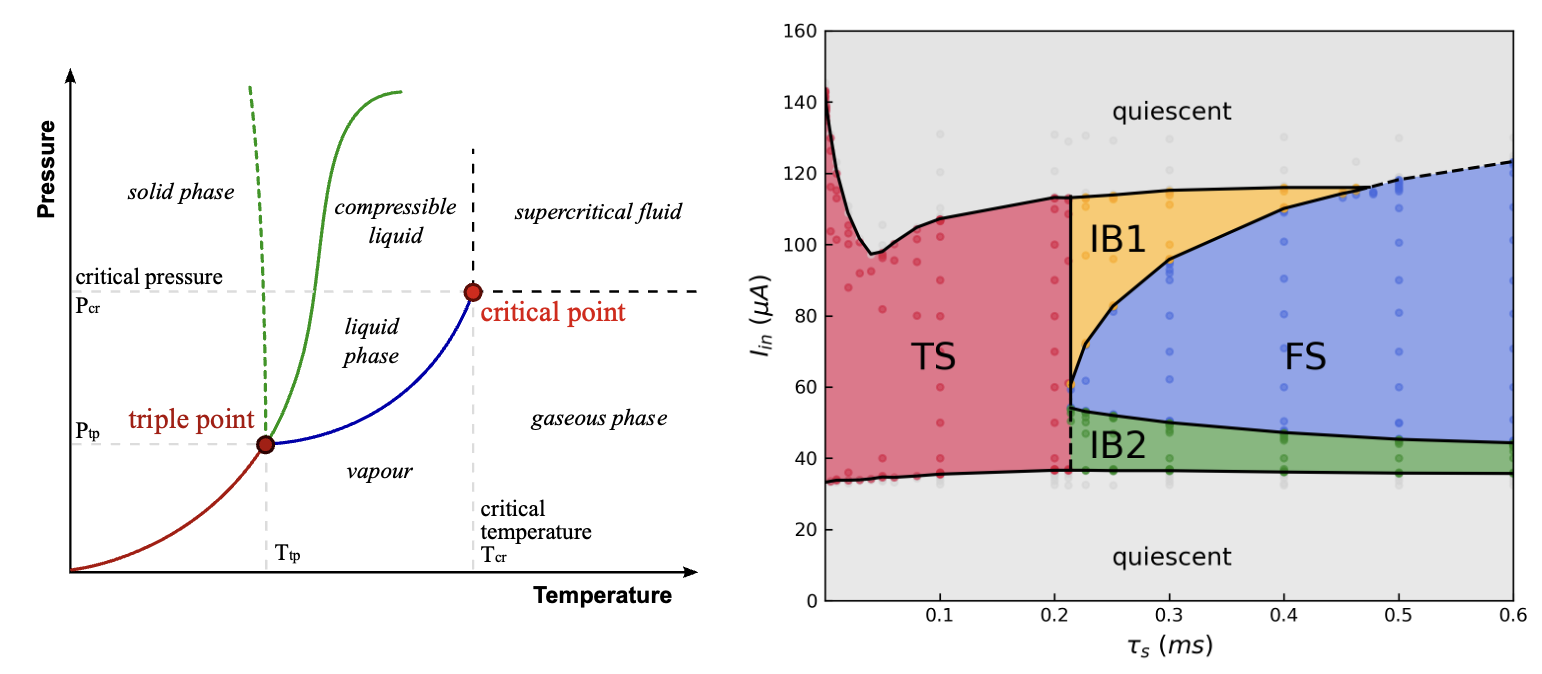
Figure 1: Left: Phase diagram of states of ordinary matter (water) showing the solid, liquid and gas phases. $P$ and $T$ determine the specific volume $v$ of the state, which is the inverse of the density $n$. Right: Measured phase diagram of temporal-matter states of an electronic neuron model. The system is a two-compartment bursting neuron, showing tonic spiking (TS), fast spiking (FS) and two different intrinsic bursting states (IB1 and IB2). The input current $I$ and the circuit time-constant $\tau_{s}$ determine the inter-spike interval of the state, which corresponds to the inverse of the frequency.

To characterize the spiking states in the phase diagram, we need to consider the nature of the discrete spiking events in the time domain. For instance, tonic spiking is characterized by a sequence of spikes that occur at equally spaced time-intervals. In Neuroscience, the time between two consecutive spike events is called the inter-spike interval (ISI). At the transition from the TS to FS phase, one observes a sudden decrease of the ISI (i.e. a jump in the spiking frequency) as function of the parameter $\tau_{s}$.

The ISI(t) characterizes the organization of the spikes in the time domain and it indicates the “time-distance” between spikes. If a sequence of spike events at times $t_{i}$ are indicated by the function

$$s(t)=\sum_{i}\delta(t-t_{i})$$ (1)

Then, it may be tempting to establish the analogy by simply identifying the time-position of spike events with the positions of particles in a matter state. The matter state is characterized by its particle density function,

$$n(x)=\sum_{i}\delta(x-x_{i})$$ (2)

where $x_{i}$ denotes the position of the $i^{th}$ particle. For simplicity, we assume point particles and one dimensional space. Similarly, in Eq.1 we have assume ideal spikes represented by $\delta$-functions, while in reality the action potentials have a typical duration of $\sim 1ms$ From the analogy, the simple tonic spiking case with equispaced spikes (i.e. constant ISI) would correspond to a perfect crystal of equally spaced particles (atoms). Thus, the familiar ISI of neuroscience would be the analogue of the familiar lattice constant $a$ (or specific volume $v$) for material science.

If one applies a pressure $P$ to matter, in general one observes the decrease of $v$, such as in the case of the Ideal Gas law $P$$v$ = constant. On the other hand, in neuroscience, it is well known that the ISI can be reduced by increasing the excitatory input current. Hence, one may be tempted to extend our analogy to associate the $P$ with the input $I$ in neural systems. We can make this more precise by introducing the simplest theoretical model of an ideal spiking neuron, the Integrate and Fire (IF) model [2].

In a very schematic view, as shown in Fig.2, a biological neuron is composed of three main parts: the dendrites, the soma and the axon. The neuron is excited through the input of electric signals arriving to the dendrites, which are called the synaptic currents. This input is integrated in the cell’s body, which leads to the increase in its electric potential with respect to its resting state. By means of intense excitation, the neuron eventually reaches a threshold potential value. At that point a dramatic event takes place, an electric spike is initiated, it propagates down the axon and eventually is communicated to the dendrites of a downstream neuron. This phenomenon is called the emission of an action potential, which was first described by Hodgkin and Huxley [4]. This qualitative description can be represented by the simple (leaky) IF model [2, 3]

$$\frac{du}{dt}=-\frac{1}{\tau}u(t)+I;\ \ if\ u\geq u_{th}\ then\ spike\ and\ u=u_{rest}$$ (3)

where $u(t)$ represents the potential of the soma, $u_{th}$ is the threshold potential, $u_{rest}$ is the resting potential value and $I$ is the input (synaptic) current. The time constant $\tau$ is a characteristic relaxation time of the neuron that represents the leakage of charge out of the soma. If the leakage is negligible, $\tau\to\infty$, and the integration is perfect, so one has an ideal IF model. The electric circuit representation of the model is straight forward. The soma is represented by a capacitor $C$ that accumulates the charge of the input current, and the leakage by a resistor $R$ in parallel. The threshold voltage can be represented by a switch that closes yielding the emission of the spike, which is the fast discharge of the charge accumulated in $C$, as a delta function of current.

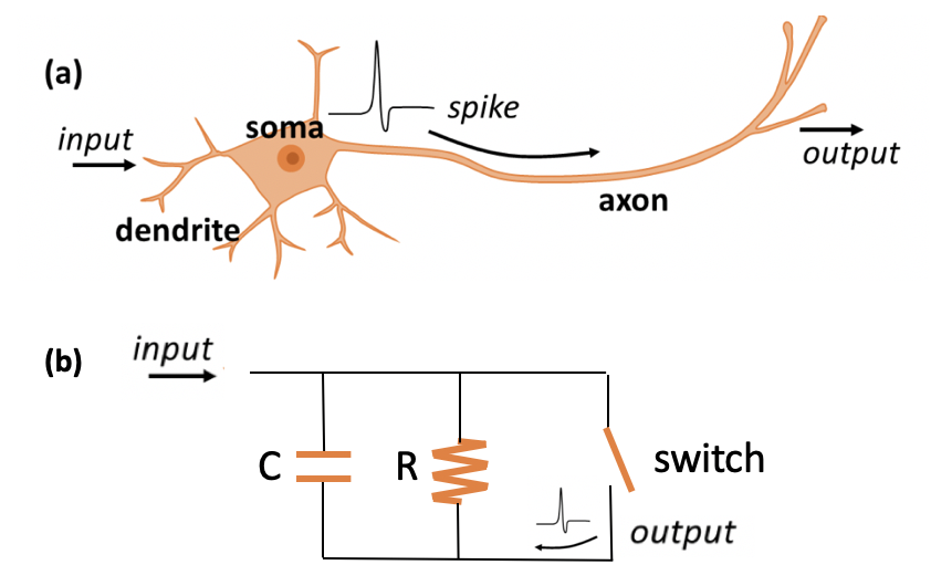
Figure 2: (a) Schematic biological neuron. (b) Electric circuit of the IF model (for the case $u_{res}$=0). The membrane of the cell’s body (soma) is represented by the capacitor $C_{m}$, which accumulates charge of the input current. If the resistor $R\to\infty$ then the current integration is perfect, however for a finite value there is a “leaky” integration and the model is called LIF, for leaky-integrate-and-fire.

The limit of zero leakage, i.e. the ideal Integrate and Fire is trivially solved. The potential $u$ due to the integrated charge in $C$ during an interval $t$ is $u(t)=Q/C=(I/C)t$. Thus, the spike fire time $t_{f}$ is given by the condition $u(t_{f})=u_{th}$. Which leads to $It_{f}=u_{th}C$, or $I{\rm ISI}=constant$.

Hence, we may extend our analogy by noting that the equation of state of the Ideal Gas has the same form as that of an ideal IF neuron, namely,

$$Pv{\rm=constant}\longleftrightarrow I{\rm ISI=constant}$$ (4)

where

$$P\longleftrightarrow I;\ \ \ v\longleftrightarrow{\rm ISI}$$ (5)

As the equation of state of a real gas departs from the ideal case, biological neurons and neuron models’ equation of state, will depart from the ideal IF “neuronal equation of state” above. Interestingly, the notion of neuronal equation of state should not appear so strange. Indeed, it is nothing else than the familiar concept in neuroscience of the neuron’s activation function, namely, the firing rate as a function of the excitatory input current, $f=f(I)$. For instance, some popular models are: the rectified linear units, or ReLU, where $f(I)=max[0,I]$; the sigmoid activation $f(I)=1/(1+e^{-I})$; etc. These are examples of mathematical neuron models, however, we may also include here physical neuron models, namely, models that are defined by an electronic circuit. In physical neuron models the equation of state $f(I)$ can be measured, as in real gases. We should mention that while the relation $Pv$= constant is familiar from the Ideal Gas law, it is in general valid for any liquid or solid in the linear regime.

Recently, we introduced a minimal model of a physical spiking neuron, which is achieved by exploiting the memristive properties of an “old” conventional electronic component, the thyristor. The model is minimal because it provides a physical realization of the basic leaky-integrate-and-fire (LIF) neuron model by associating exactly one component to each one of the three functions: a capacitor to integrate, a resistor to leak and the thyristor to fire. Qualitatively, the thyristor acts as the switch in the circuit of Fig.2.

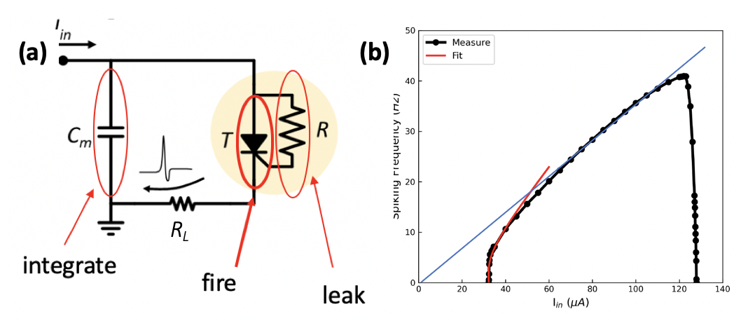
Figure 3: (a) Electric circuit that defines the physical neuron model based on the memristive properties of the thyristor. The function of the thyristor is that of a voltage controlled switch, as shown in Fig.2 above. The small “load” resistor $R_{L}$ is to transform the output spike current into a voltage action potential signal for measurement convenience. (b) The “neuron equation of state” or activation function $f(I)$. Near the threshold, the equation of state follows closely the functional form of a LIF model (red line),  $-1/[log(1-I_{c}/I)]$ where $I_{c}$ is the minimal activation current. The blue line corresponds to the Ideal IF behavior $I\propto$ 1/ISI$\ =f$.

In Fig.3 we show the circuit that defines physical neuron model just described, where we identify the role of each of the three components to the functions of the LIF. We call this artificial neuron model the Memristive Spiking Neuron (MSN), which is implicitly defined by its electronic circuit. In the right panel of the figure we show the experimental neuron equation of state, which is nothing other than the activation function, as noted above. We can observe that near the excitation threshold the equation of state is well represented by the functional form of the activation function of the LIF mathematical model (red fitting line in Fig.3). At intermediate input currents, the behavior approaches the Ideal IF neuron, whose equation of state is $f\propto I$ (see 4), since $f=1/ISI$

The same methodology allows us to consider more complex neuron models, which are also defined by their respective circuit implementation. For instance, we may consider the case of bursting neurons. From theoretical neuroscience we know that a requirement to obtain bursting behavior is by adding a second dynamical variable, besides the potential of the cell body $u(t)$, in Eq.4 and represented by the capacitor in the circuits of Fig.2 and 3. Thus, to do this we add a second $RC$ pair to our basic MSN circuit. A simple option is to add a capacitor $C_{L}$ in parallel to the (small) output resistor $R_{L}$, introducing a new time constant $\tau_{L}=R_{L}C_{L}$. The resulting circuit is shown in Fig.4a. In panel (b) we show the dynamical behavior that it now produces. We observe four qualitatively different spiking types: simple tonic spiking, fast spiking, and two bursting modes. These four spiking types are realized in the respective regions of the phase diagram of Fig.1 presented before.

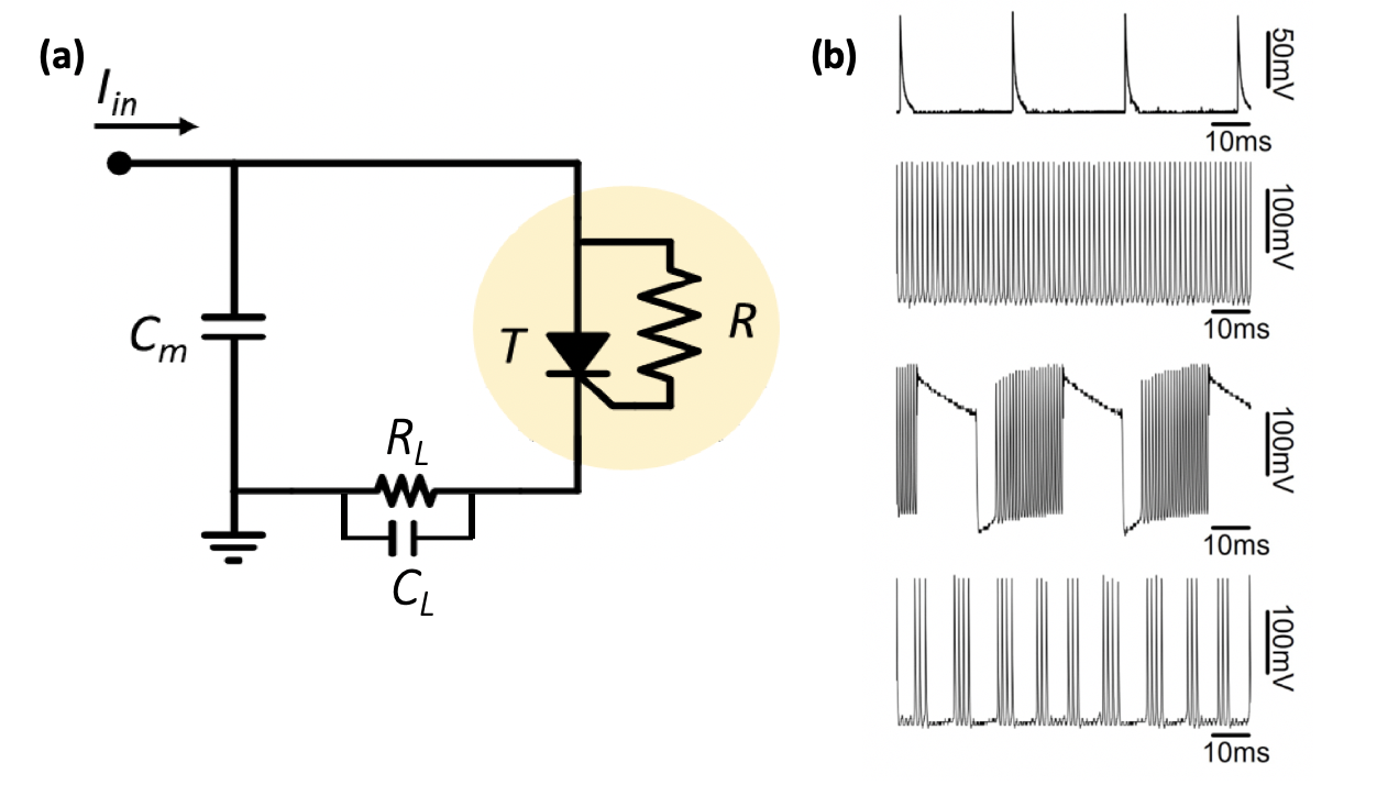
Figure 4: (a) Electric circuit that defines the physical model of a bursting neuron based on the MSN model and adding a second time constant $\tau_{L}=R_{L}C_{L}$. (b) The various dynamical behaviors produced by the circuit. From top to bottom: tonic spiking (TS), fast spiking (FS) and two bursting types (IB1, IB2), which correspond to the four phases of the phase diagram shown in Fig.1.

As done before for the basic MSN, we may also obtain the equation of state of the Memristor Bursting Neuron (MBN) model. In the present case, we can consider that the time constant $\tau_{L}$ plays the role of a third parameter, similarly as the temperature in the case of matter systems. Hence, in Fig.5 we show the curve $f_{\tau_{L}}(I)$ measured at a fixed $\tau_{L}$, indicated by the vertical purple line that crosses three phases. We observe the jumps in the frequency as the current drives the system from one phase to the other. This is reminiscent of changes in density when the pressure drives phase transitions at a fixed $T$ in the phase diagram of water in Fig.1.

It is interesting to mention that a biologically realistic theoretical model of bursting neurons introduced by Pinsky and Rinzel (PR) shows a qualitatively similar behavior [9]. The PR is an example of a two-compartment model, where both the soma and the dendrites are described. We may notice that in the MBN model the $R_{L}C_{L}$ block (see Fig.4) can be considered as a second compartment, which is connected to the output of the first. In the right panel of Fig.5, we reproduce the activation function (i.e. the neuronal equation of state) of the PR model. It is interesting to observe that in the simpler limits of only one compartment (soma alone and dendrite alone) the behavior of the PR is qualitatively the same as that of our basic MSN, which is also a single compartment model (see bottom curve of Fig.5a). More importantly, for the relevant case of two compartments (i.e. finite $g_{c}$) we observe a sudden changes in the firing rate as a function of excitatory input current, also in qualitative agreement with the MBN. In fact, both PR and MBN traverse the same sequence as the excitatory current is increased: initially quiescent below a critical current, then bursting, and finally jump in firing rate to the fast spiking mode. Hence, the phase transitions are abrupt, through a steep or a discontinuous change in the activation function. As we shall discuss in the next section this feature may have interesting consequences. Moreover, and we shall show that the $f(I)$ anomalies may be considered as the counterparts of certain phenomena occurring in phase transitions in matter systems.

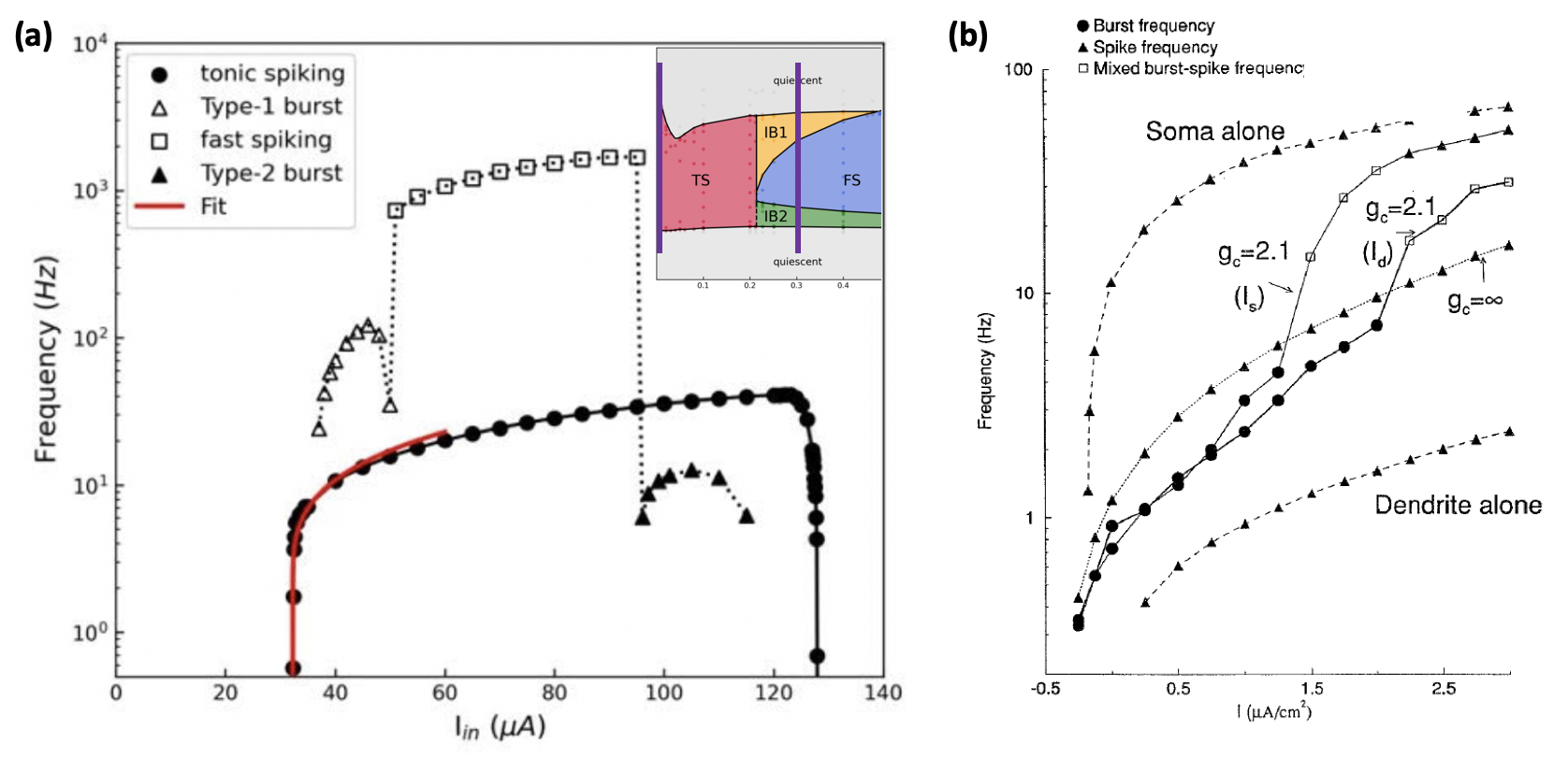
Figure 5: (a) Activation function $f(I)$ in semilog scale. The top curve corresponds to the MBN model along the right purple line at $\tau_{L}$=0.3ms indicated in the phase diagram in the inset. Following the definition of Pinsky and Rinzel, the frequency is defined as the inverse of the period between spike trains (bursts). The bottom $f(I)$ curve is that of the MSN model discussed before, which corresponds to the limit $\tau_{L}\to 0$ of the bursting neuron model (indicated with the left purple line in the inset). (b) Activation function of the Pinsky-Rinzel model reproduced from [9].

III Correlation and Response Functions

Correlation and response functions are useful concepts in material science, where they serve to characterize different states of matter. For instance, a regularity in the arrangement of positions of atoms is revealed by Bragg peaks in the x-ray spectra, which are maxima of the structure factor. In real space, the regularity is revealed by the pair correlation function

$$g({x})=\frac{\int n(x+x^{\prime})n(x^{\prime})dx^{\prime}}{\int n^{2}(x^{\prime})dx^{\prime}}$$ (6)

where $n(x)$ indicates the particle density (such as electrons, atoms, molecules, etc) at position $x$, and where we consider one dimension for simplicity. In the case of a crystalline order, $g(x)$ shows structure with peaks. For a simple arrangement of particles along one dimension with a lattice constant $a$, the peaks will be at $a$, $2a$, $3a$, … In contrast, for a disordered state, such as gas or liquid, the $g(x)$ is mostly featureless. The study of $g(x)$ is routinely done in condensed matter physics for the study of phase transitions (see, for example, [10]).

In our analogy, spiking systems are thought of as temporal-matter states, so it is natural to explore the behavior of the correlation-function analogue to $g(x)$. Since the position of particles correspond to position of spikes, by analogy we can define the neural correlation function $g_{n}(t)$ as

$$g_{n}(t)=\frac{\int s(t+t^{\prime})s(t^{\prime})dt^{\prime}}{\int s^{2}(t^{\prime})dt^{\prime}}$$ (7)

where $s(t)$ indicates a given spike trace. The function $g_{n}(t)$ can characterize different spiking states of a neuron. In Fig.6 we provide a concrete example, which is realized in the basic MSN model described before (see Fig.3).

Figure 6: (a) Measured spike traces $s(t)$ of the MSN model at two values of the input current: a “solid” state measured at $I$ = 45.3$\mu$A (top) and a “melted” state at $I$ = 36.4$\mu$A. The states are indicated with the green and blue dots in the activation function of the neuron reproduced in the inset. (b) The neural correlation function $g_{n}(t)$ computed for the respective traces shown in the left side panels (only a small portion of the measured traces is shown).

We can observe the two qualitatively different tonic spiking behaviors in the two left panels of the figure. They correspond to two constant current inputs (36.4$\mu$A and 45.3$\mu$A). In the first case, at higher input current (top panel), the spiking is perfectly regular. In contrast for a smaller current close to the threshold, the trace changes dramatically. The interval between spikes become very irregular. By analogy between spike and particles, we can think of the first case as that of a solid and the second as of the melting of the solid state. This qualitative description can be made more precise by the correlation function $g_{n}(t)$, shown on the right side panels of Fig.6.

The top panel shows a succession of delta functions at equally spaced at times, multiples of the constant inter-spike interval, $t_{k}$=$k$ISI. This indicates the long range order in time. It tells that given the presence of a spike at time $t=0$ we have a high probability (  1) of finding another spike event at times $t_{k}$ ($k$=1, 2, 3, …). In contrast, the $g_{n}(t)$ shown in the bottom panel is featureless, showing a small approximate constant value. This indicates total lack of order as the presence of a spike a time $t=0$ does not permit to predict the presence of ulterior spikes events. The emission of spikes is random as the positions of particles in a liquid or a gas.

The peaks of the $g_{n}(t)$ are very narrow, delta-function-like, because the spikes are very narrow with respect to the duration of the ISI. In a solid, the atoms have a size that is smaller but of the same order as the lattice spacing, so instead of narrow deltas one observes broad peaks in the $g(x)$ [10].

One may understand quite intuitively the physical origin of this dramatic changes in the time-structure. The key point is to realize that the “melted” state occurs in a regime where the activation function $f(I)$ is very steep, at the onset of neuron excitability, i.e. near the threshold. Therefore, small variations of the input current will reflect on significant variations in the ISI. This observation motivates the following important insight.

This enhanced sensitivity to current fluctuations is due to the large slope $df/dI$ in the activation function. Then, what is this feature related to, if one follows the analogy back to the matter systems? We recall that ISI plays the role of the lattice spacing, or specific volume (see Eqs.4 and 5), then $f$=1/ISI corresponds the particle density $n(x)=1/v(x)$. On the other hand, since the input current $I$ is like the pressure, then it follows that the slope $df/dI$ corresponds to $dn/dP$. This last quantity is closely related to the compressibility of matter systems

$$\beta=\frac{1}{n}\ (\frac{dn}{dP})$$ (8)

which is the inverse of the bulk modulus. We can therefore follow the analogy and introduce the concept of “neuro-compressibility”,

$$\beta_{n}=\frac{1}{f}\ (\frac{df}{dI})$$ (9)

It is important to mention that this quantity may be measured using experimental methods such as dynamic clamp, where a controlled synaptic current can be injected into a neuron while its activity is monitored [11]. Moreover, this definition may turn out to have important consequences, as we discuss next.

Anomalies in the compressibility of materials are precursor signatures of structural phase transitions. A sudden increase in the compressibility of a solid indicates the “softening” of a vibrational mode (a phonon mode), which leads to a change in the structure, or possibly a phase change. Then, the question is, what would the analogue phenomenon be for a neuronal system? For a single neuron, the enhancement of $\beta_{n}$ would indicate the proximity to a qualitative change in the spiking mode of a neuron, i.e. a “bifurcation” in its dynamics. This can in fact be seen in the panels of Fig.5. There, we observe that all the changes in the spiking modes for both, the MSN and for the MBN models, occur at current values where there are enhancements in $df/dI$ or jumps. Most notably, this is not only a feature of our artificial neuron circuits, but also can be clearly seen in the biologically realistic Pinsky-Rinzel model activation functions that we reproduced in Fig.5 [9]. The enhancements seen in the PR data occur at the onset of change from quiescent to spiking and also in the change from burst to tonic spiking (black circles and black triangles), in very good qualitative agreement to our electronic neuron model,

We may then speculate on an important implication of our observations. It would be interesting to explore if neuro-compressibility anomalies are also found across the boundaries of qualitatively different states in neuron networks. If that is the case, an intriguing and exciting possibility would be to investigate if anomalies in $\beta_{n}$ are also detected (by small current stimulation) in animal models of epilepsy and Parkinson’s disease. If this were the case, then one may envision a pathway to a novel diagnose tool for early detection or a risk predictor of mental diseases associated to abnormal spike patterns in humans. In even further speculation, one may also search for anomalies at the onset of regaining, or loosing, consciousness, which is another challenging frontier of research [12].

IV Bursting spikes as an ananlogue of formation of clusters defects

Here we describe another interesting connection between common a phenomena in spiking neurons and in material science. We shall show that missing spikes in a trace of a fast spiking state, can be thought of as the analogue of missing atoms, i.e, defects, in a crystal structure.

From Fig.7 we observe that the proliferation of missing spikes in a fast spiking state is a route to generate bursting behavior. This is illustrated in the sequence of traces shown in the figure, which were obtained for a step-wise decreasing input current to the MBN. The thick purple arrow in the vertical path followed in phase diagram (from blue to green to grey). In the top trace we indicate with small purple arrows the missing arrows, showing that one may understand the onset of bursting as the result of skipping spike events, which are initially few (i.e. dilute). As the current intensity is further reduced, the missing spikes become more numerous (i.e dense) and occurring in clusters of inactivity, which give rise to the stuttering mode bursts [13]. In our analogy, we think of spikes as of atoms in a lattice, therefore, the initial continuous fast spiking state is like a perfect crystal. The missing spikes then play the analogue role as vacancy defects, i.e. lacking atoms. Moreover, the missing spikes are the result of decreasing current, which in the analogy represents pressure. It is then interesting to observe that in thin-film deposition, which is a topic in material science, the partial pressure of oxygen $P$(O₂) is a relevant parameter for the quality of the growth of crystalline oxides. Moreover, it is well known that reducing the $P$(O₂) induces the creation of oxygen vacancy defects in the crystal structure [14, 15], which often cluster together forming dislocations [16], This is in full qualitative analogy to the spiking traces in the stuttering bursting mode shown in Fig.7.

We would like to emphasize that the path of phase transformations, i.e. the evolution from fast spiking, to bursting, to quiescent does not seem to be just a peculiarity of our MBN circuit model. In the lower panel of the Fig.7 we illustrate the striking resemblance of the traces of the MBN with those measured in bursting neuron of rats [17]. Quite remarkably, the experimental traces were obtained by solely changing the intensity of the excitatory DC current.

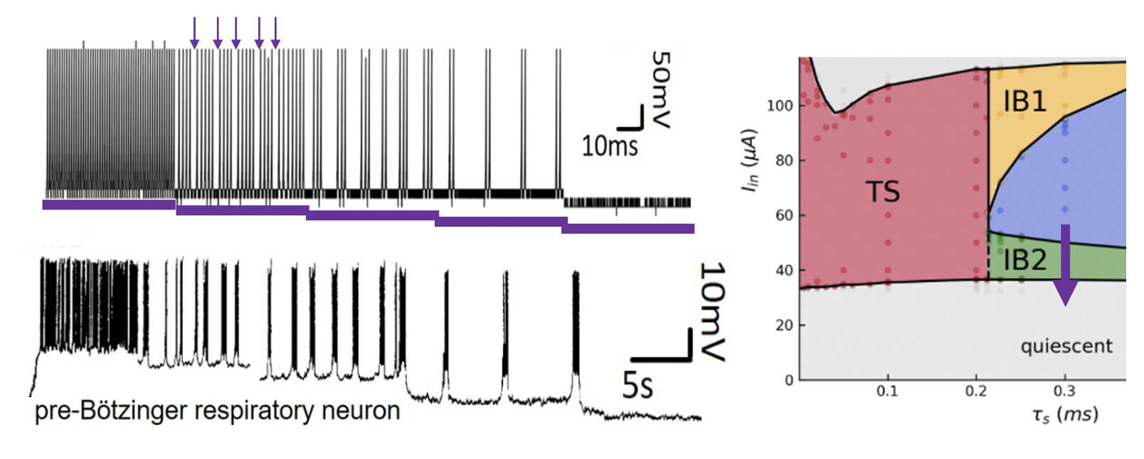
Figure 7: Top left: Measured spike traces of the MBN as a function of decreasing current in discrete steps (purple). The thin purple arrows indicate the missing spikes. Bottom left: Experimental trace of pre-Bötzinger bursting neurons from rats. The data is obtained by changing excitatory input current in discrete steps. Adapted from [17]. The circuit parameters may be easily adjusted to fit the experimental data [8]. Right: Phase diagram of the MBN where the purple arrow indicates the evolution from the fast spiking (blue) to the bursting type 1 phase (green) by decreasing current at constant $\tau_{L}$.

V Neural Networks

We now consider one important final aspect in our analogy that may eventually bring new light to the issue of how to think about inter-neuron coupling. So far we have considered essentially individual neurons, but we may ask what would it be to extend the analogy to multi-neuron systems, i.e. to neural networks.

As a first glimpse into this question, we shall consider the simplest network case, namely, just two neurons that are mutually excitatory or inhibitory. We focus first in a system of two identical neurons, each excited with equal input currents. The currents are above threshold, so the neurons are active and theirs spikes are transformed via conductances into mutually injected synaptic currents that are positive for the excitatory case and negative for the inhibitory one. This is schematically shown in Fig.8.

We shall see that our analogy takes an interesting twist, as the dynamical states of the two-neuron system can be considered as an analogue of a complex crystal, i.e. a crystal with two atoms in the unit cell. Moreover, the coupling between neurons is mediated by synaptic currents, which can be excitatory or inhibitory. Since in our analogy current plays the role of pressure, then the synaptic currents should also play such a role. More precisely, an excitatory synaptic current should correspond to a repulsive inter-particle interactions (positive pressure), and an inhibitory synaptic current should be an attractive interaction (negative pressure). We shall consider the two cases, which we study using realistic electronic circuit simulations (LTspice).

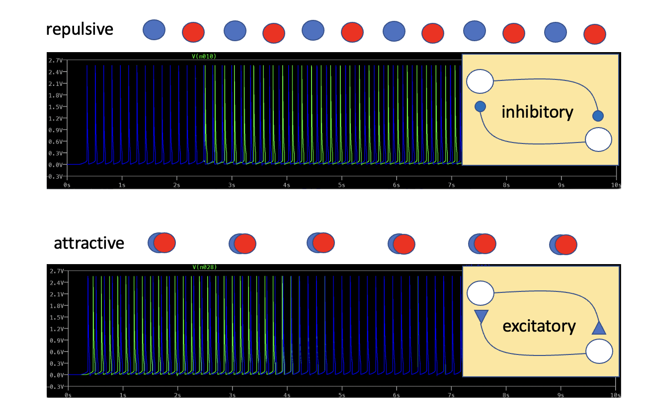
Figure 8: Top: two 1D space lattices (red and blue) with repulsive interaction and two neurons with inhibitory interactions. The neurons are prepared to start spiking synchronously and spontaneously adopt an alternating spiking pattern. Bottom: two 1D lattices with attractive interactions and two neuron network with excitatory interaction. They are prepared to alternate but spontaneously begin to spike in unison. Spike traces were produced by realistic simulations with LTSpice.

We first consider two spiking neurons with mutual inhibition. When one neuron spikes it inhibits the other, and vise-versa, so they try to avoid spiking at unison since we are synaptic current are instantaneous. After a transient period, they expectedly find a stable dynamical state where they alternate to emit spikes as shown in the top panel of Fig.8. Using our analogy, this spiking pattern corresponds two a perfect molecular crystal where the unit cell has an A-B atom pair (or a basis).

In the bottom panel of the figure we consider the second case, that of mutually excitatory neurons. Again after a transient time, the system adopts a periodic spiking pattern. However, in contrast to the previous case, now both neurons fire at unison. This is also intuitive, the excitatory synaptic current of emitted by a neuron that spiked promotes the spiking of the other one, and vise versa. So, naturally, the both spike at the same time, which is nothing else that excitatory synapses promote synchrony in neural networks [18]. Following our analogy, spiking at unison corresponds to a “dimerization” of the lattice. Namely, that the distance between the A-B pair atoms is reduced as due to an attractive interaction between the A and B atomic species.

These two cases are consistent with our analogy, where current is interpreted as pressure. Indeed, the volume of the unit cell in the inhibitory case is large, as expected for positive effective pressure between A and B, while in the excitatory case the volume is fully collapsed to zero, as expected for a negative pressure within the unit cell.

It is an interesting perspective for future work to consider increasingly complex networks of several neurons (motifs). The periodic states that emerge constitute spiking sequences, which are of great relevance for automatic motor behavior. By virtue of the analogy that we introduced in the present work, those periodic sequences should correspond to a variety of molecular crystals. It would be exciting to explore if new intuition for Neuroscience could be brought from from those traditional areas of Condensed Matter Physics and Chemistry [19].

VI Conclusion

In this work we introduced the idea that the dynamical states of neural networks may be though of as realizations of “time matter” states.

We started from the notion that a trace of spiking events of a neuron can be analogue to a snapshot of particles or atoms arranged in space. We then went on to explore and show that the analogy may be pushed far beyond that literary statement, and may provide new intuition in the challenging problem of understanding and designing spiking neural networks.

We identified analogue roles of basic quantities of Physics with those of Neuroscience, such as pressure and volume with input currents and inter-spike intervals. We then logically build on this assumption to show connections between correlation and response functions in both fields. Perhaps most significant was the finding that a neuro-compressibility can be defined, with possible far reaching consequences, including medical ones, that may be experimentally tested.

An exciting new road of discovery may open ahead.

VII Acknowledgments

We acknowledge support from the French ANR “MoMA” project ANR-19-CE30-0020.

References

- Bear et al. [2016] M. Bear, B. Connors, and M. Paradiso, Neuroscience: Exploring the Brain (Wolters Kluwer, Philadelphia, 4Th ed. international ed., 2016).
- Gerstner et al. [2014] W. Gerstner, W. Kistler, R. Naud, and L. Paninski, Neuronal Dynamics: From Single Neurons to Networks and Models of Cognition (Cambridge University Press, 2014).
- Ermentrout and Terman [2010] G. Ermentrout and D. Terman, Mathematical Foundations of Neuroscience, Interdisciplinary Applied Mathematics (Springer New York, 2010).
- Hodgkin and Huxley [1952] A. L. Hodgkin and A. F. Huxley, A quantitative description of membrane current and its application to conduction and excitation in nerve, The Journal of Physiology 117, 500 (1952).
- Hopfield [1982] J. J. Hopfield, Neural networks and physical systems with emergent collective computational abilities, Proceedings of the national academy of sciences 79, 2554 (1982).
- LeCun et al. [2015] Y. LeCun, Y. Bengio, and G. Hinton, Deep learning, Nature 521, 436 (2015).
- Merolla et al. [2014] P. A. Merolla, J. V. Arthur, R. Alvarez-Icaza, A. S. Cassidy, J. Sawada, F. Akopyan, B. L. Jackson, N. Imam, C. Guo, Y. Nakamura, et al., A million spiking-neuron integrated circuit with a scalable communication network and interface, Science 345, 668 (2014).
- Wu et al. [2023] J. Wu, O. Schneegans, K. Wang, P. Stoliar, and M. Rozenberg, submitted (2023).
- Pinsky and Rinzel [1994] P. F. Pinsky and J. Rinzel, Intrinsic and network rhythmogenesis in a reduced traub model for ca3 neurons, Journal of Computational Neuroscience 1, 39 (1994).
- Debela et al. [2014] T. T. Debela, X. D. Wang, Q. P. Cao, Y. H. Lu, D. X. Zhang, H.-J. Fecht, H. Tanaka, and J. Z. Jiang, Nucleation driven by orientational order in supercooled niobium as seen via ab initio molecular dynamics, Phys. Rev. B 89, 104205 (2014).
- Goaillard and Marder [2006] J.-M. Goaillard and E. Marder, Dynamic clamp analyses of cardiac, endocrine, and neural function, Physiology 21, 197 (2006), pMID: 16714478.
- Storm et al. [2017] J. F. Storm, M. Boly, A. G. Casali, M. Massimini, U. Olcese, C. M. A. Pennartz, and M. Wilke, Consciousness regained: Disentangling mechanisms, brain systems, and behavioral responses, The Journal of Neuroscience 37, 10882 (2017).
- Golomb et al. [2007] D. Golomb, K. Donner, L. Shacham, D. Shlosberg, Y. Amitai, and D. Hansel, Mechanisms of firing patterns in fast-spiking cortical interneurons, PLOS Computational Biology 3, e156 (2007).
- Ghenzi et al. [2015] N. Ghenzi, M. J. Rozenberg, R. Llopis, P. Levy, L. E. Hueso, and P. Stoliar, Tuning the resistive switching properties of tio2-x films, Applied Physics Letters 106, 123509 (2015).
- Liu et al. [2009] X. Liu, K. Zhou, L. Wang, B. Wang, and Y. Li, Oxygen vacancy clusters promoting reducibility and activity of ceria nanorods, Journal of the American Chemical Society 131, 3140 (2009).
- Szot et al. [2006] K. Szot, W. Speier, G. Bihlmayer, and R. Waser, Switching the electrical resistance of individual dislocations in single-crystalline srtio3, Nature Materials 5, 312 (2006).
- Butera et al. [1999] R. J. J. Butera, J. Rinzel, and J. C. Smith, Models of respiratory rhythm generation in the pre-bötzinger complex. i. bursting pacemaker neurons., J Neurophysiol 82, 382 (1999).
- Hansel et al. [1995] D. Hansel, G. Mato, and C. Meunier, Synchrony in Excitatory Neural Networks, Neural Computation 7, 307 (1995).
- Corpinot and Bučar [2019] M. K. Corpinot and D.-K. Bučar, A practical guide to the design of molecular crystals, Crystal Growth & Design 19, 1426 (2019).