Quantum work statistics at strong reservoir coupling

Abstract

Calculating the stochastic work done on a quantum system while strongly coupled to a reservoir is a formidable task, requiring the calculation of the full eigenspectrum of the combined system and reservoir. Here we show that this issue can be circumvented by using a polaron transformation that maps the system into a new frame where weak-coupling theory can be applied. It is shown that the work probability distribution is invariant under this transformation, allowing one to compute the full counting statistics of work at strong reservoir coupling. Crucially this polaron approach reproduces the Jarzynski fluctuation theorem, thus ensuring consistency with the laws of stochastic thermodynamics. We apply our formalism to a system driven across the Landau-Zener transition, where we identify clear signatures in the work distribution arising from a non-negligible coupling to the environment. Our results provide a new method for studying the stochastic thermodynamics of driven quantum systems beyond Markovian, weak-coupling regimes.

In macroscopic thermodynamics, the energy of the interaction between a system and a thermal environment is dwarfed by their respective bulk energies. Consequently, the interaction contribution to energy changes like heat and work can be safely ignored, and the equilibrium state of the system can be adequately described by a thermal Gibbs state at the same temperature as the environment. However, the weak coupling approximation becomes less well founded when we consider the thermodynamics of mesoscopic and quantum mechanical systems in which the interaction terms can become more comparable to the system’s energy scale Jarzynski (2017). As recent advancements in quantum control now makes this regime experimentally accessible Potočnik et al. (2018); Maier et al. (2019); Takahashi et al. (2020), there is significant interest in exploring how non-negligible interactions and structured environments can modify the equilibrium behaviour and thermodynamic laws of strongly coupled quantum systems Ingold et al. (2008); Strasberg et al. (2016); Perarnau-Llobet et al. (2018); Hsiang et al. (2018); Gelbwaser-Klimovsky and Aspuru-Guzik (2015); Strasberg (2019); Rivas (2020); Talkner and Hänggi (2020).

The first key deviation from standard thermodynamics lies in the fact that the equilibrium state of the system generally differs from the familiar Gibbs state when weak coupling breaks down. Studies of both exactly-solvable and approximate models of strongly coupled quantum systems provide evidence that, when left to equilibriate, the system reaches the partial trace of a global Gibbs state with respect to both system and environment Grabert et al. (1984); Subasi et al. (2012); Thingna et al. (2012); Cresser and Anders (2021); Trushechkin et al. (2022). This motivates the introduction of the so-called mean-force free energy $F_{S}^{*}$ Ford et al. (1985); Jarzynski (2004); Gelin and Thoss (2009); Philbin and Anders (2016); Miller (2018), which is an effective thermodynamic potential for the system that determines its properties at equilibrium while encoding information about interactions with the environment. This generalised notion of free energy also acts as the main ingredient for extending the laws of stochastic thermodynamics to the strong coupling regime out of equilibrium. For example, one can derive an extension of the Jarzynski fluctuation theorem when a system is driven away from a non-Gibbsian equilibrium state Campisi et al. (2009a):

$$\big{\langle}e^{-\beta W}\big{\rangle}=e^{-\beta\Delta F_{S}^{*}}.$$ (1)

Here $W$ denotes the work done on the open system, $\langle.\rangle$ denotes an average with respect to the work distribution $P(W)$, and $\Delta F_{S}^{*}$ denotes the change in the mean-force free energy of the system at inverse temperature $\beta$. While formally correct, the difficulty in verifying this theorem lies in the fact that the work distribution $P(W)$ is formidably difficult to compute in strong-coupling regimes since it is obtained from projecting the total system and environment into global energy eigenstates at the start and end of the process Campisi et al. (2009a); Talkner et al. (2009); Talkner and Hänggi (2020). Ultimately this has led to work statistics at strong coupling receiving little attention, with the exception of relatively few exactly solvable models Campisi et al. (2009b); Schmidt et al. (2015); Aurell (2017); Funo and Quan (2018). One significant issue is that numerically exact techniques for simulating open system dynamics, such as discrete time path-integral methods Makri and Makarov (1995); Strathearn et al. (2018); Cygorek et al. (2022), are formulated to describe the dynamics of the reduced state of the system, and therefore do not have straightforward access to the eigenspectrum of the composite system and environment required to construct the full work distribution.

In this paper we introduce an alternative approach based on the polaron framework Nazir (2009); Jang et al. (2008); McCutcheon and Nazir (2011) that is not hampered by these issues. The polaron method uses a unitary transformation to dress system states with vibrational modes of the environment, capturing the dominant non-Markovian effects and allowing the system-environment interaction to be included non-perturbatively. The polaron framework has been successfully adapted to study resonant energy transfer in photosynthetic complexes Kolli et al. (2011); Jang (2011), exciton-phonon interactions in semiconductor quantum dots McCutcheon and Nazir (2010), and heat exchange statistics in the time-independent spin-boson model with multiple reservoirs Wang et al. (2015); Popovic et al. (2021). Within the polaron transformed frame, we are able to derive a generalised master equation (GME) that governs the evolution of the characteristic function associated with $P(W)$ beyond weak coupling regimes. This can be used to infer the full statistics of work and reproduces the fluctuation theorem (1) as required for thermodynamic consistency. To demonstrate our approach, we consider a Landau-Zener (LZ) driving protocol on the system Hamiltonian. We find that stronger coupling creates new peaks in the distribution as well as imparting significant broadening and renormalisation, indicating clear signatures in the work statistics arising from interactions with the reservoir that are either not captured or severely underestimated by a weak-coupling approach.

Generalised Master Equation for Quantum Work– We begin by considering a general time-dependent spin-boson model, governed by the Hamiltonian,

$$H(t)=H_{S}(t)+H_{R}+\sigma_{z}\otimes\sum_{k}g_{k}(b_{k}^{\dagger}+b_{k}),$$ (2)

where the time-dependent system Hamiltonian is given by

$$H_{S}(t)=\frac{1}{2}\omega_{0}(t)\sigma_{z}+\frac{1}{2}\Delta\sigma_{x}.$$ (3)

Here $\omega_{0}(t)$ is a time-varying energy spacing and $\Delta$ is a fixed tunneling coefficient. The reservoir Hamiltonian is given by $H_{R}=\sum_{k}\omega_{k}b_{k}^{\dagger}b_{k}$, with $b_{k}$ the annihilation operator for the $k$th mode of frequency $\omega_{k}$. The final term in Eq. 2 describes the system-resevoir interaction mediated by a set of scalar coupling constants $g_{k}$. This interaction is fully characterised by the spectral density $J(\omega)=\alpha\omega_{c}^{-2}\omega^{3}\exp(-\omega/\omega_{c})$, with cutoff frequency $\omega_{c}$ and $\alpha$ a measure of the interaction strength. The composite state at a time $t$ is given by the density operator $\rho(t)=U(t)\rho(t_{i})U^{\dagger}(t)$ with initial state $\rho(t_{i})$ and time-ordered unitary $U(t)=\overleftarrow{\mathcal{T}}\text{exp}\big{(}-i\int^{t_{f}}_{t_{i}}dt^{\prime}H(t^{\prime})\big{)}$.

We now wish to compute the statistics of work done on the system during the driving protocol, that is we are interested in the total energetic change of the system and environment during the protocol, including any stochastic fluctuations of these quantities. Independent of the coupling strength, the work done can be defined using the two-point measurement protocol, where a projective energy measurement of the global Hamiltonian (2) is made at the initial and final times of the protocol, with the work done $W$ defined as the resulting energy difference Campisi et al. (2009a). The resulting distribution $P(W)$ can be characterised by its characteristic function (CF), given by its Fourier transform

$$\Phi(\eta)=\int^{\infty}_{-\infty}e^{i\eta W}P(W)dW=\tr{K(t_{f},\eta)}.$$ (4)

Here we define the work characteristic operator (WCO) Talkner et al. (2007),

$$K(t_{f},\eta):=e^{i\eta H(t_{f})}U(t_{f})e^{-i\eta H(t_{i})}\bar{\rho}(t_{i})U^{\dagger}(t_{f}),$$ (5)

where $\bar{\rho}(t_{i})=\sum_{n}\Pi^{i}_{n}\rho(t_{i})\Pi^{i}_{n}$ is the initial state dephased in the energy eigenbasis of $H(t_{i})$, with $\Pi^{i}_{n}$ a projector onto the $n$th eigenstate. Without further approximations, computing the CF even numerically is challenging due to the presence of the interaction term in (2). One immediate solution would be to assume the interaction is sufficiently weak, allowing one to derive a Lindblad-like master equation for the WCO (5) Esposito et al. (2009); Silaev et al. (2014); Suomela et al. (2015); Liu and Xi (2016). However, our aim is to probe regimes where this approximation is not appropriate, and so we require an alternative method for computing $K(t,\eta)$. Our approach is to use the fact that we are free to apply a trace-preserving operation to the WCO such as $K(t_{f},\eta)\mapsto K_{P}(t_{f},\eta)=e^{P}K(t_{f},\eta)e^{-P}.$ This will always leave the CF invariant so that $\Phi(\eta)=\tr{K_{P}(t_{f},\eta)}$. For our spin-boson model we choose the unitary polaron transformation McCutcheon and Nazir (2011), where $P=\sigma_{z}\otimes\sum_{k}(g_{k}/\omega_{k})(b_{k}^{\dagger}-b_{k})$. This transformation redraws the boundary between the system and environment by dressing the system states with vibrational modes of the environment. By moving into the polaron frame, we can account for a significant part of the interaction using these dressed system states, and the residual part of the interaction in this frame can be treated perturbatively. The transformed WCO is given by $K_{P}(t_{f},\eta)=e^{i\eta H_{P}(t_{f})}U_{P}(t_{f})e^{-i\eta H_{P}(0)}\bar{\rho}_{P}(t_{i})U_{P}^{\dagger}(t_{f}),$ where $\bar{\rho}_{P}(t_{i})=e^{P}\bar{\rho}(t_{i})e^{-P}$ and $U_{P}(t)=\overleftarrow{\mathcal{T}}\text{exp}\big{(}-i\int^{t_{f}}_{t_{i}}dt^{\prime}H_{P}(t^{\prime})\big{)}$ is the evolution operator with respect to the polaron-transformed Hamiltonian

$$H_{P}(t):=e^{P}H(t)e^{-P}=H_{PS}(t)+H_{R}+V_{P}.$$ (6)

Here we identify the polaron system Hamiltonian

$$H_{PS}(t)=\frac{1}{2}\omega_{0}(t)\sigma_{z}+\frac{1}{2}\Delta\kappa\sigma_{x},$$ (7)

where $0\leq\kappa\leq 1$ denotes the polaron renormalisation constant that lowers the tunneling coefficient of our transformed system. The degree of renormalisation is dependent on the structure of the reservoir, and can be computed from its spectral density according to

$$\kappa:=\exp\bigg(-2\int^{\infty}_{0}d\omega\frac{J(\omega)}{\omega^{2}}\coth\big(\beta\omega/2\big{missing})\bigg{missing}).$$ (8)

Furthermore, we have identified a new interaction term in the polaron frame given by

$$V_{P}=\frac{\Delta}{2}\bigg{(}\sigma_{x}\otimes\xi_{x}+\sigma_{y}\otimes\xi_{y}\bigg{)},$$ (9)

where $\xi_{x}=\frac{1}{2}(\xi_{+}+\xi_{-})-\kappa$ and $\xi_{y}=\frac{i}{2}(\xi_{+}-\xi_{-})$, with $\xi_{\pm}=\Pi_{k}D(\pm\alpha_{k})$. This new interaction can now be treated in a perturbative manner quantified by the parameter McCutcheon and Nazir (2011)

$$g:=\frac{\Delta}{2}\sqrt{(1+\kappa^{4})/2}.$$ (10)

Taking a weak-coupling approximation in this new frame will allow us to determine the work statistics of driven systems that are strongly coupled to the reservoir with respect to the original frame.

Let us assume that the system and environment have initially thermalised to a global Gibbs state with respect to the Hamiltonian in the original frame, $\rho(t_{i})=\pi^{eq}(t_{i}):=e^{-\beta H(t_{i})}/\tr{e^{-\beta H(t_{i})}}$ with $\beta=1/k_{B}T$ an inverse temperature. As our first approximation we suppose that the interaction strength in the polaron frame is weak enough relative to the reservoir temperature so that $\beta^{2}g^{2}\ll 1$. We can then neglect any correlations in the initial state and contributions of the interaction to the initial and final energy measurements, so that the polaron transformed WCO simplifies to

$$K_{P}(t_{f},\eta)\simeq e^{i\eta(H_{PS}(t_{f})+H_{B})}U_{P}(t_{f})e^{-i\eta(H_{PS}(t_{i})+H_{B})}$$

$$\ \ \ \ \ \ \ \ \ \ \ \ \ \times\big{(}\pi^{eq}_{PS}(t_{i})\otimes\pi^{eq}_{R}\big{)}U_{P}^{\dagger}(t_{f}),$$ (11)

where $\pi^{eq}_{R}$ is a Gibbs state of the bare reservoir with Hamiltonian $H_{R}$ while $\pi^{eq}_{PS}(t_{i})$ is a Gibbs state of the polaron system with the initial Hamiltonian $H_{PS}(t_{i})$. We emphasise that this approximation is valid in strong coupling regimes, unlike the typical weak coupling limit in which $\rho(t_{i})\simeq\pi^{eq}_{S}(t_{i})\otimes\pi^{eq}_{R}$ Talkner et al. (2009).

To obtain the work statistics we derive a master equation for the WCO of the system degrees of freedom in the polaron frame, which is obtained by taking a partial trace over the reservoir so that $K_{PS}(t_{f},\eta)=\text{Tr}_{\scriptscriptstyle R}\big{[}K_{P}(t_{f},\eta)\big{]}$. The derivation of an equation for the evolution of $K_{PS}(t_{f},\eta)$ then follows similar steps used to obtain an adiabatic master equation for the polaron state itself, and details are provided in Appendix A. This rests on a number of assumptions such as $(i)$ the Born-Markov approximation, stating that the coupling in the polaron frame is much smaller than the inverse of the decay time of the reservoir correlation function and $(ii)$ the adiabatic approximation, which ensures that the system Hamiltonian does not change too rapidly in time relative to its energy gaps and bath correlation time. Note that applying the Born-Markov approximation in the polaron frame is not equivalent to applying it in the original frame, and retains the dominant non-Markovian effects in the dynamics. Under these assumptions the general form of equation for the polaron WCO is then

$$\partial_{t}K_{PS}(t,\eta)=\mathcal{L}_{t}[K_{PS}(t,\eta)]+\mathcal{W}(t,\eta)[K_{PS}(t,\eta)],$$ (12)

where we define the work superoperator

$$\mathcal{W}(t,\eta)(.)=\big{[}\partial_{t}e^{i\eta H_{PS}(t)}\big{]}e^{-i\eta H_{PS}(t)}(.),$$ (13)

and $\mathcal{L}_{t}(.)=-i[H_{PS}(t)+H_{PLS}(t),(.)]+\mathcal{D}_{t}(.)$ is an adiabatic Lindblad generator with $H_{PLS}(t)$ the polaron lamb shift and $\mathcal{D}_{t}(.)$ the dissipator, which are both derived and defined in Appendix B. Physically, the dissipator drives transitions between the instantaneous energy eigenstates of the polaron system, defined as $\ket{\varepsilon_{+}(t)}=\cos(\theta_{t}/2)\ket{1}+\sin(\theta_{t}/2)\ket{0}$ and $\ket{\varepsilon_{-}(t)}=-\sin(\theta_{t}/2)\ket{1}+\cos(\theta_{t}/2)\ket{0}$ with $\theta_{t}=\arctan(\Delta\kappa/\omega_{0}(t))$ and energy eigenvalues $\varepsilon_{\pm}(t)=\pm\frac{1}{2}\omega(t)$, where $\omega(t)=\sqrt{\omega_{0}(t)^{2}+\kappa^{2}\Delta^{2}}$ is the transition frequency. This contrasts with the standard weak-coupling master equation (WCME) for time-dependent driving Albash et al. (2012), whose dissipator causes transitions between eigenstates of the original system Hamiltonian $H_{S}(t)$ (see Appendix B).

A key property of this generator is that it has an instantaneous thermal fixed point so that

$$\mathcal{L}_{t}[\pi^{eq}_{PS}(t)]=0;\ \ \ \ \pi^{eq}_{PS}(t)=\frac{e^{-\beta H_{PS}(t)}}{\text{tr}_{PS}\big{[}e^{-\beta H_{PS}(t)}\big{]}}.$$ (14)

Taking the trace of the solution to (12) for a given protocol with an initial condition set to $K_{PS}(t_{i},\eta)=\pi^{eq}_{PS}(t_{i})$ finally allows us to calculate the work CF. As a main consistency check, our formalism can be used to recover the quantum fluctuation theorem in the strong coupling regime Campisi et al. (2009a). In particular, one may combine the fixed point property (14) with our chosen initial conditions to show that $K_{PS}(t_{f},i\beta)=e^{-\beta H_{PS}(t_{f})}/\text{tr}_{PS}\big{[}e^{-\beta H_{PS}(t_{i})}\big{]}$ is a solution to (12). This immediately implies the quantum Jarzysnki equality

$$\big{\langle}e^{-\beta W}\big{\rangle}=e^{-\beta\Delta F_{PS}},$$ (15)

where $\Delta F_{PS}=F_{PS}(t_{f})-F_{PS}(t_{i})$ is the change in the polaron system free energy

$$F_{PS}(t) =-k_{B}T\ln\ \text{tr}_{PS}\big{[}e^{-\beta H_{PS}(t)}\big{]},$$

$$=-k_{B}T\ln\bigg(2\ \text{cosh}\bigg{[}\frac{\beta}{2}\sqrt{\omega_{0}^{2}(t)+\kappa^{2}\Delta^{2}}\bigg{]}\bigg{missing}).$$ (16)

Here we may interpret this quantity as an approximation to the original system’s mean-force free energy Campisi et al. (2009a); Miller (2018); Jarzynski (2017), defined by

$$F_{S}^{*}(t):=F_{SR}(t)-F_{R},$$ (17)

which is the difference between the total free energy $F_{SR}(t)=-\beta^{-1}\text{ln}\ \text{tr}\big{[}e^{-\beta H(t)}\big{]}$ of the composite state and the free energy of a bare reservoir, $F_{R}=-\beta^{-1}\text{ln}\ \text{tr}_{R}\big{[}e^{-\beta H_{R}}\big{]}$. It then follows from our approximation $\beta^{2}g^{2}\ll 1$ that the polaron free energy is equal to this mean force free energy to the same order in coupling; $F_{PS}(t)\simeq F_{S}^{*}(t)$ and hence we have recovered the Jarzynski equality (1) obtained within the original frame. From the validity of the fluctuation theorem, one can therefore conclude that the work distribution predicted by our equation (12) is consistent with the laws of stochastic thermodynamics Talkner and Hänggi (2020).

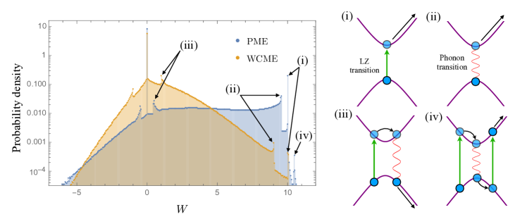
Figure 1: Left: Probability distribution of the dissipative LZ model as given by polaron (PME) and weak-coupling (WCME) generalised master equations. The CF step width is $\delta\eta=0.05$, the maximum counting-field value is $\eta_{\text{max}}=500$, and the bin width is $\delta W=0.05\Delta$. Other parameters are $\nu=0.1\Delta^{2}$, $t_{0}=-100/\Delta$, $t_{f}=100/\Delta$, $\alpha=0.4$, $\beta=1/\Delta$, $\omega_{c}=10\Delta$. The horizontal axis is in units of $\Delta$. Right: (i-iv) show the mechanisms leading to the labelled peaks in the probability distribution.

It is important to highlight the parameter regimes for which our model is valid; to do this, we shall consider the specific case of a two level system driven over a Landau-Zener crossing. In this case, the time dependent driving in the Hamiltonian may be written as $\omega_{0}(t)=\nu t$, where $\nu$ is the rate at which the driving occurs. First we consider the Born-Markov approximation in the polaron frame, which amounts to assuming that the environment can respond instantaneously to the dynamics of the system, where the dynamical timescale of the reservoir is proportional to the cutoff frequency $\omega_{c}$. From (10) this requires McCutcheon and Nazir (2011)

$$\frac{\Delta}{2\omega_{c}}\sqrt{(1+\kappa^{4})/2}\ll 1.$$ (18)

So long as we have a sufficiently large cutoff frequency $\Delta\ll\omega_{c}$, this condition can be satisfied from low to high temperatures, and from weak to strong coupling as defined by the original frame (small to large $\alpha$). This provides us with a much wider parameter regime to probe the work statistics than would be possible with the WCME. Second, to ensure that the adiabatic approximation holds for the time-dependent protocol, we need the rate of change of the polaron’s eigenbasis to be small relative to the energy gaps of its Hamiltonian. This is achieved when

$$\max_{t\in[t_{i},t_{f}]}\frac{\Delta\kappa\nu}{2(\nu^{2}t^{2}+\Delta^{2}\kappa^{2})^{3/2}}=\frac{\nu}{2\Delta^{2}\kappa^{2}}\ll 1,$$ (19)

where $t_{i}$ and $t_{f}$ are the initial and final times respectively Yamaguchi et al. (2017). The maximum is found at the intermediate avoided crossing where $t=0$. If we compare this condition with the Born-Markov condition (18), we see that this can be maintained at any temperature so long as we choose a large enough cutoff frequency $\omega_{c}$. As a final condition we also require that the rate of change of the polaron energy eigenbasis must be small relative to the reservoir dynamics Albash et al. (2012); Mozgunov and Lidar (2020); Dai et al. (2022); Chen and Lidar (2022), which means $\nu\ll 2\omega_{c}$; this is guaranteed if the previous conditions are satisfied. To confirm that polaron theory gives a faithful description of the reduced system, we have benchmarked the system population dynamics using the numerically exact TEMPO method Strathearn et al. (2018) in Appendix C and find excellent agreement with the adiabatic polaron dynamics at strong coupling, in contrast to the WCME. Therefore, we conclude that in the Landau-Zener model our master equation for the WCO Eq. (12) is accurate so long as $\Delta\ll\omega_{c}$ and $\nu\ll 2\Delta^{2}\kappa^{2}$.

Work Statistics— We now numerically solve the master equation (12) for the Landau-Zener model. In all following calculations, we choose $\nu=0.1\Delta^{2}$ and start and end the protocol far from the avoided crossing $-t_{0}=t_{f}=100$, this ensures that the adiabatic condition is satisfied. To ensure the validity of the PME we work in the scaling limit $\Delta/\omega_{c}\ll 1$ Nazir and McCutcheon (2016); McCutcheon and Nazir (2010), taking $\omega_{c}=10\Delta$. To calculate the work distributions we sample the CF via the solution to the generalised PME (12) over a range of counting-field values at intervals $\delta\eta$ up to some cut-off $\eta_{\text{max}}$, before performing a numerical inverse Fourier transformation on this data to obtain the work probability density function. A discrete work probability distribution is then found by numerically integrating the probability density over fixed intervals $\delta W$.

Before considering the work statistics of the full open quantum system, it is worth briefly discussing the expected behaviour for a closed system. If we start the system in the thermal state, such that the initial thermal occupation of the ground state is $p_{-}=1/(1-e^{-\beta\omega})$, then we expect there to be three possible contributions to the work distribution: if the system’s trajectory remains adiabatic there is no net change in the energy of the system, and therefore no work is done. This occurs with probability $P(W=0)=1-P_{LZ}$, where $P_{LZ}=1-\exp{-\pi\Delta^{2}/2\nu}$ is the LZ transition probability. If a LZ transition occurs, as shown in Fig. 1(i), the system can move from its ground to excited state. The work done on the system is given by the net energy change $W=\Delta E=(\omega_{0}(t_{f})-\omega_{0}(t_{i}))/2$, and occurs with probability $P(W=\Delta E)=p_{-}P_{LZ}$. As the system is initially in thermal equilibrium, the converse process may also occur, where a LZ transition occurs between the excited and ground states, extracting $W=-\Delta E$ of work. This occurs with probability $P(W=-\Delta E)=(1-p_{-})P_{LZ}$, and is expected to be heavily suppressed if the LZ protocol is initialised far from the avoided crossing.

Now let’s consider the more interesting case of the open quantum system. In Fig. 1 we show polaron and weak-coupling predictions for the quantum work distribution for a choice of $\alpha$ well into the strong coupling regime. The most immediate difference in the open system distribution is that it is continuous in contrast to the discrete distribution of the closed system. Since the bath is composed of a continuum of modes, it may exchange energy with the system at any of the continuous range of transition frequencies that the system moves through during the protocol.

In analogy to the closed system, both the polaron and weak-coupling distributions show a peak at $W=0$ and $W=\Delta E$ corresponding to the adiabatic and non-adiabatic system trajectories (again, see Fig. 1(i) for a schematic of the latter process ). Interestingly, non-adiabatic transitions are over two orders of magnitude more likely to occur in the polaron formalism versus the weak-coupling approach. This is a direct consequence of the renormalisation of the energy gap to $\Delta\kappa$, with $\kappa$ given by Eq. (8), meaning that the system dynamics must be slower to maintain the same degree of adiabaticity.

Unlike the closed system, both the weak-coupling and polaron probability distributions show a much richer structure due to phonon mediated processes. The simplest phonon process is shown schematically in Fig. 1(ii), where a phonon excites the system over the avoided crossing, which then continues to evolve adiabatically in the excited state. This requires $W=\Delta E-\Delta\approx 9\omega(t_{f})$ of work in weak coupling theory, which is reduced to $W=\Delta E-\Delta\kappa\approx 9.5\omega(t_{f})$ for the polaron approach due to the renormalisation of the avoided crossing.

The peaks in the distribution either side of the origin, which are due to a heat exchange event at the avoided crossing in combination with a nonadiabatic transition (Fig. 1(iii)), can be interpreted similarly and are brought closer together in the PME due to renormalisation. While renormalisation tends to shift such peaks, we also observe that strong coupling tends to increase the likelihood of larger amounts of work being done on the system. One explanation for this is routed in the fact that, as mentioned, non-adiabatic transitions are less suppressed in the PME, as can be seen from its larger adiabatic parameter (19) when compared with the WCME (for which $\kappa=1$). From a thermodynamic perspective, this leads to a greater probability of excitation and thus an increased likelihood of dissipation, which here corresponds to larger amounts of work being done to the system. As a final observation, the polaron approach predicts another type of process not apparent in the weak coupling theory and given schematically by Fig 1(iv), whereby a LZ transition excites the system, which emits a phonon, before a second LZ transition re-excites the system. The total work done in this situation is $W=\Delta E+\Delta\kappa\approx 10.5\omega(t_{f})$.

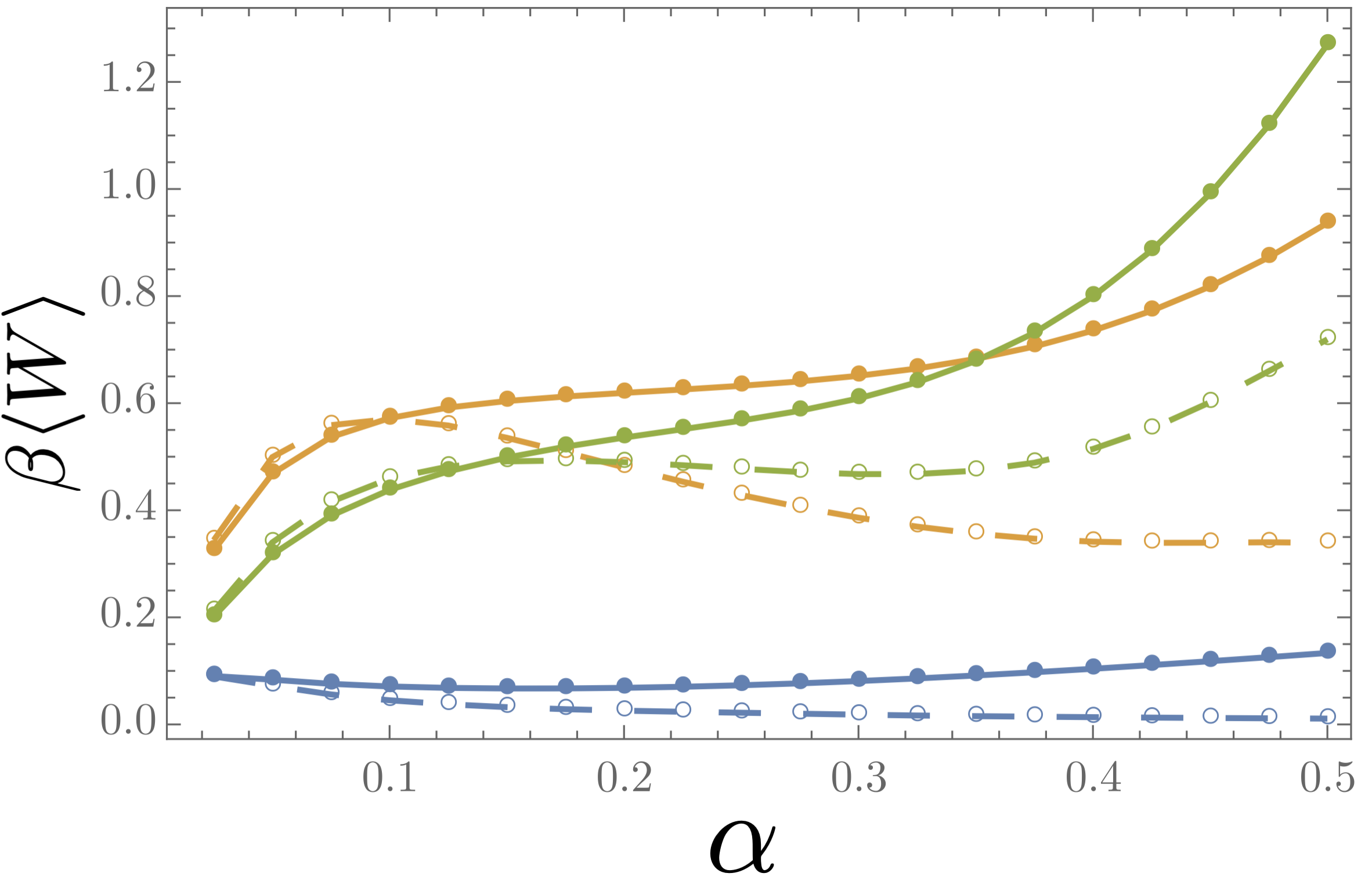
(a)

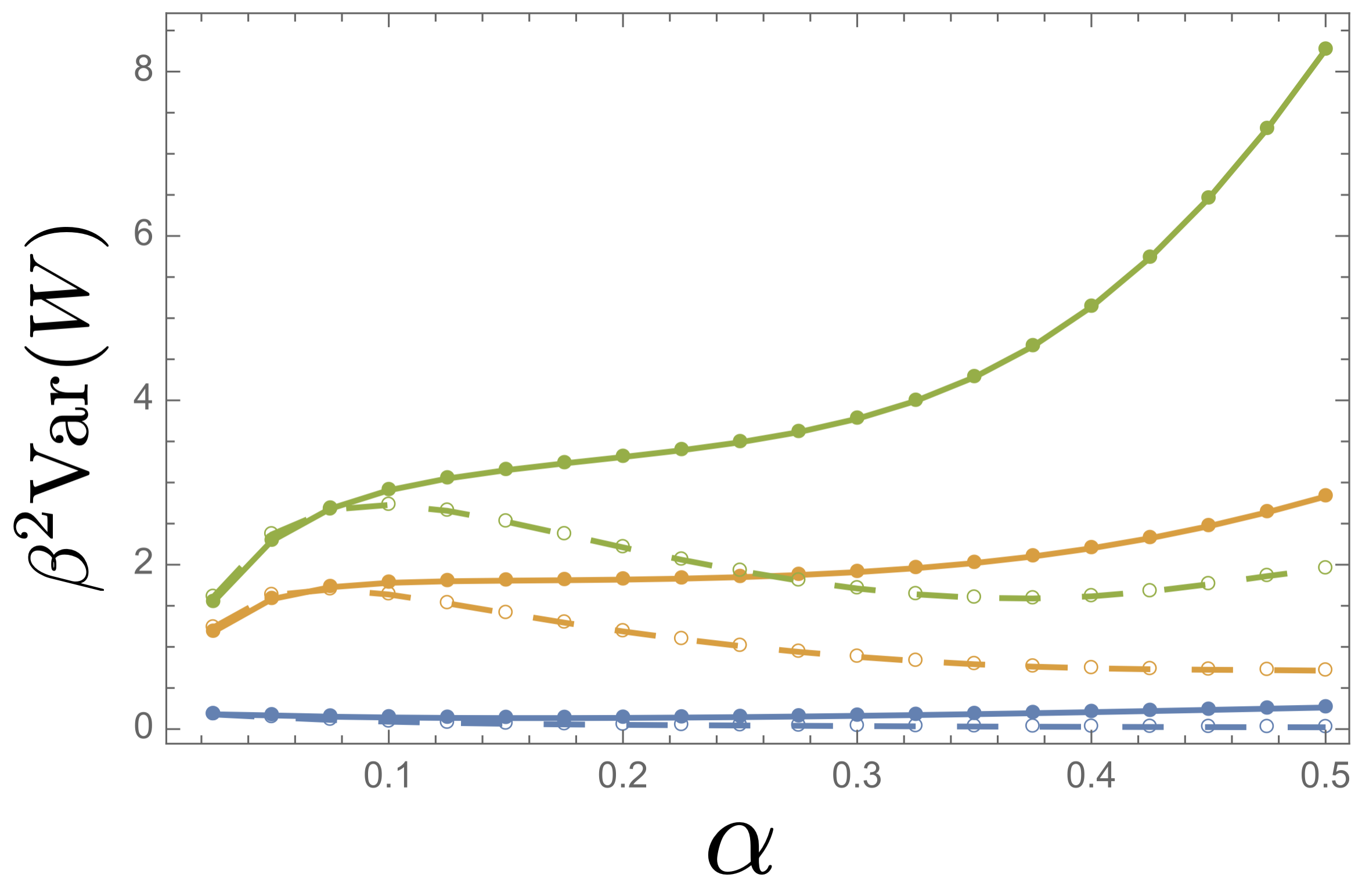
(b)

Figure 2: Average work done per $k_{B}T$ (top) and work variance per $k_{B}^{2}T^{2}$ (bottom) given by polaron (solid line and solid markers) and weak-coupling (dashed line and open markers) GMEs as a function of the coupling strength $\alpha$. We plot results for the inverse temperature fixed at $\beta=1/(5\Delta)$ (blue), $\beta=1/(2\Delta)$ (orange), and $\beta=1/\Delta$ (green). Other parameters are as in Figure 1.

We can also observe how the increased likelihood of stochastic dissipation of the system in the PME impacts both the average and fluctuations in work done. Figure 2 displays the average work $\expectationvalue{W}$ and variance $\operatorname{var}(W)=\expectationvalue{W^{2}}-\expectationvalue{W}^{2}$ calculated by the PME as functions of the coupling and inverse temperature, and compared to the corresponding predictions from the standard weak-coupling model. Since there is no change in the free-energy of the system-bath from the beginning to end of the protocol, any work done is dissipative. We see that for this range of coupling strengths and temperatures, the weak-coupling theory typically underestimates the average work and its variance, with this discrepancy only becoming negligible at small coupling and low temperature.

To summarise our findings, we see clear differences between predictions of the WCME and PME at the level of full work statistics. The stronger coupling manifests in the work distribution by shifting the positions of various peaks associated with both adiabatic and non-adiabatic transitions due to a renormalisation of the system Hamiltonian. Furthermore, higher coupling tends to drive the system further from equilibrium due to the increased level of non-adiabaticity in the PME. This results in an increased likelihood of stochastic work done on the system and leads to significant increases in the average dissipation and work fluctuations when compared to predictions from the weak coupling approach.

Conclusion— We have studied the full-counting statistics of work done in the time-dependent spin-boson model beyond the weak coupling regime and have derived a generalised master equation for the corresponding WCO (5). This has been achieved by exploiting the unitary invariance of the work characteristic function, from which it was possible to apply the polaron transformation to rotate the WCO into a new frame where we could revert to standard approximations from weak-coupling theory. This resulted in the master equation (12) that can be solved to give the full work probability distribution in parameter regimes where the standard Markovian model breaks down, such as strong coupling. We illustrated our general approach by solving the dissipative Landau-Zener model, where the polaron framework indicated significant increases in both average dissipation and work fluctuations in contrast to predictions from the weak coupling master equation. This serves to highlight the limitations of the usual weak-coupling approximation, as even modest increases in the coupling can have a noticeable impact on the stochastic thermodynamics of the system.

Our results lay the groundwork for further investigations into how correlations, non-Markovianity Schmidt et al. (2015) and other strong coupling effects can influence the full statistics of work in driven open quantum systems. The polaron framework could be applied to study higher order work fluctuations in thermal machines beyond weak coupling such as quantum Otto cycles Newman et al. (2017) and Carnot engines Gelbwaser-Klimovsky and Aspuru-Guzik (2015). It could also provide a route towards free energy estimation in strongly coupled systems via the fluctuation theorem (15). In principle, one could apply quantum jump unravelling techniques Hekking and Pekola (2013); Horowitz and Parrondo (2013) with respect to the polaron renormalised Hamiltonian to record the work statistics, which in turn could be used to establish estimates of the mean force free energy change using standard methods Gore et al. (2003); Park et al. (2003).

We conclude by noting a number of ways in which our approach could be generalised. Firstly, the polaron transformation that we have used is restricted to reservoirs with super-Ohmic spectral densities. However, this could be straightforwardly generalised using variational polaron theory Silbey and Harris (1984), which allows treatment of both Ohmic and sub-Ohmic spectral densities, as has been used recently to study heat transport in non-equilibrium steady states Hsieh et al. (2019). Furthermore, the unitary invariance of the work characteristic function allows for other transformations such as the reaction coordinate mapping Nazir and Schaller (2018). This approach could provide a means for computing work statistics in other strongly coupled systems, such as linearly coupled oscillators and fermionic environments.

Acknowledgements. O. D. acknowledges the EPSRC for PhD funding support, H. M. acknowledges funding from the Royal Commission for the Exhibition of 1851. We thank Ali Raza Mirza for helpful discussions.

Appendix A Deriving the WCO master equation

In this section we provide a derivation of the equation (12) starting from the polaron-transformed WCO in (Quantum work statistics at strong reservoir coupling). We write the interaction Hamiltonian (9) in a generic form

$$V_{P}=\sum_{a}A_{a}\otimes B_{a},$$ (20)

where are $A_{a}(B_{a})$ Hermitian system (bath) operators. The derivation closely follows a projection operator approach used by Liu (2018) to obtain an equation for the WCO with a standard weak-coupling adiabatic master equation. We start by differentiating (Quantum work statistics at strong reservoir coupling) and find that it satisfies the differential equation

$$\partial_{t}K_{P}(t,\eta)=-i\big{[}H_{P}(t),K_{P}(t,\eta)\big{]}-i\big{[}e^{i\eta(H_{PS}(t)+H_{R})},V_{P}\big{]}e^{-i\eta(H_{PS}(t)+H_{R})}K_{P}(t,\eta)+\left[\partial_{t}e^{i\eta H_{PS}(t)}\right]e^{-i\eta H_{PS}(t)}K_{P}(t,\eta).$$ (21)

with the initial condition $K_{P}(0)=\sum_{i,j}\Pi_{ij}(0)\rho(0)\Pi_{ij}(0)$, where $\rho_{P}(0)$ is the initial density matrix of the system-bath in the polaron frame and $\Pi_{ij}$ is the projection operator at the initial time that projects onto the eigenspace corresponding to the polaron frame system eigenenergy $\varepsilon_{i}(0)$ and the bath eigenenergy $\varepsilon^{B}_{j}$ i.e.

$$H_{PS}\Pi_{ij}(0) =\varepsilon_{i}(0)\Pi_{ij}(0),$$ (22)

$$H_{B}\Pi_{ij}(0) =\varepsilon^{B}_{j}(0)\Pi_{ij}(0).$$ (23)

To simplify notation we define a set of superoperators:

$$\mathcal{V}(t)[\cdot] \equiv-i[H_{P}(t),(\cdot)],$$ (24)

$$\mathcal{J}_{\eta}(t)[\cdot] =-i\big{[}e^{i\eta(H_{PS}(t)+H_{R})},V_{P}\big{]}e^{-i\eta(H_{PS}(t)+H_{R})}(\cdot),$$ (25)

$$\mathcal{W}_{\eta}(t)[\cdot] =[\partial_{t}e^{i\eta H_{PS}(t)}]e^{-i\eta H_{PS}(t)}(\cdot),$$ (26)

where the subscript $\eta$ denotes a dependence on the counting parameter. Next we move into to the interaction picture with respect to $H_{0}(t)=H_{PS}(t)+H_{R}$ and write the evolution equation as

$$\partial_{t}\tilde{K}_{P}(t,\eta)=\left[\tilde{\mathcal{V}}(t)+\tilde{\mathcal{J}}_{\eta}(t)+\tilde{\mathcal{W}}_{\eta}(t)\right]\tilde{K}_{P}(t,\eta).$$ (27)

where we indicate the interaction picture with a tilde. To get the reduced dynamics we will introduce the Nakajima-Zwanzig projection operators defined by:

$$\mathcal{P}O =\text{Tr}_{\scriptscriptstyle R}\big{[}O\big{]}\otimes\pi^{eq}_{R},$$ (28)

$$\mathcal{Q}O =[\mathds{1}-\mathcal{P}]O.$$ (29)

Due to the fact that $\text{Tr}_{\scriptscriptstyle R}\big{[}B_{a}\pi_{R}^{eq}\big{]}=0\ \ \forall a$ , we have

$$\mathcal{P}\tilde{\mathcal{W}}_{\eta}(t)=\tilde{\mathcal{W}}_{\eta}(t)\mathcal{P}$$ (30)

$$\mathcal{P}\tilde{\mathcal{J}}_{\eta}(t)\mathcal{P}=0$$ (31)

$$\mathcal{P}\tilde{\mathcal{V}}(t)\mathcal{P}=0$$ (32)

Now, applying the projection operators to (27), and using these properties we have

$$\partial_{t}\mathcal{P}\tilde{K}_{P}(t,\eta) =\mathcal{P}\left[\tilde{\mathcal{V}}(t)+\tilde{\mathcal{J}}_{\eta}(t)\right]\mathcal{Q}\tilde{K}_{P}(t,\eta)+\tilde{\mathcal{W}}_{\eta}(t)\mathcal{P}\tilde{K}_{P}(t,\eta),$$ (33)

$$\partial_{t}\mathcal{Q}\tilde{K}_{P}(t,\eta) =\left[\mathcal{Q}\left(\tilde{\mathcal{V}}(t)+\tilde{\mathcal{J}}_{\eta}(t)\right)+\tilde{\mathcal{W}}_{\eta}(t)\right]\mathcal{Q}\tilde{K}_{P}(t,\eta)+\mathcal{Q}\left(\tilde{\mathcal{V}}(t)+\tilde{\mathcal{J}}_{\eta}(t)\right)\mathcal{P}\tilde{K}_{P}(t,\eta).$$ (34)

The solution to the homogeneous version of the second equation is

$$[\mathcal{Q}\tilde{K}_{P}(t,\eta)]_{c}=\tilde{G}(t,s)\mathcal{Q}\tilde{K}_{P}(0,\eta),$$ (35)

where we have introduced the superpropagator

$$\tilde{G}(t,s)=\overleftarrow{\mathcal{T}}\text{exp}\bigg{(}\int^{t}_{s}du\left[\mathcal{Q}\left(\tilde{\mathcal{V}}(u)+\tilde{\mathcal{J}}_{\eta}(u)\right)+\tilde{\mathcal{W}}_{\eta}(u)\right]\bigg{)}.$$ (36)

To get the particular solution to the nonhomogeneous equation, we first multiply the complimentary solution from the right by an unknown operator $C(t)$:

$$[\mathcal{Q}\tilde{K}_{P}(t,\eta)]_{p}=\tilde{G}(t,0)\mathcal{Q}\tilde{K}_{P}(0,\eta)C(t).$$ (37)

Substituting this in to (34), we get the differential equation

$$\tilde{G}(t,0)\mathcal{Q}\tilde{K}_{P}(0,\eta)C^{\prime}(t)=\mathcal{Q}\left(\tilde{\mathcal{V}}(t)+\tilde{\mathcal{J}}_{\eta}(t)\right)\mathcal{P}\tilde{K}_{P}(t,\eta).$$ (38)

We solve this equation for $C(t)$ to find the particular solution

$$[\mathcal{Q}\tilde{K}_{P}(t,\eta)]_{p}=\int^{t}_{0}ds\ \tilde{G}(t,s)\mathcal{Q}[\tilde{\mathcal{V}}(s)+\tilde{\mathcal{J}}_{\eta}(s)]\mathcal{P}\tilde{K}_{P}(s,\eta),$$ (39)

where we have used the composition rule for the superpropagator $\tilde{G}(t,s)=\tilde{G}(t,0)\tilde{G}^{-1}(s,0)$ and have chosen the arbitrary initial condition $C(0)=0$. The general solution to the nonhomogeneous equation is

$$\begin{split}\mathcal{Q}\tilde{K}_{P}(t,\eta)&=[\mathcal{Q}\tilde{K}_{P}(t,\eta)]_{c}+[\mathcal{Q}\tilde{K}_{P}(t,\eta)]_{p}\\ &=\tilde{G}(t,s)\mathcal{Q}\tilde{K}_{P}(0,\eta)+\int^{t}_{0}ds\ \tilde{G}(t,s)\mathcal{Q}\left[\tilde{\mathcal{V}}(s)+g\tilde{\mathcal{J}}_{\eta}(s)\right]\mathcal{P}\tilde{K}_{P}(s,\eta).\end{split}$$ (40)

We now choose the initial condition $\mathcal{Q}\tilde{K}_{P}(0,\eta)=0$, which is true for an initial separable state, to get $\mathcal{Q}\tilde{K}_{P}(t,\eta)=\int^{t}_{0}ds\ \tilde{G}(t,s)\mathcal{Q}[\tilde{\mathcal{V}}(s)+\tilde{\mathcal{J}}_{\eta}(s)]\mathcal{P}\tilde{K}_{P}(s,\eta)$. Substituting this solution in to the first differential equation (33) we have

$$\partial_{t}\mathcal{P}\tilde{K}(t,\eta)=\tilde{\mathcal{W}}_{\eta}(t)\mathcal{P}\tilde{K}_{P}(t,\eta)+\mathcal{P}[\tilde{\mathcal{V}}(t)+\tilde{\mathcal{J}}_{\eta}(t)]\int^{t}_{0}ds\ \tilde{G}(t,s)\mathcal{Q}[\tilde{\mathcal{V}}(s)+\tilde{\mathcal{J}}_{\eta}(s)]\mathcal{P}\tilde{\mathcal{U}}(s,t)\tilde{K}_{P}(t,\eta),$$ (41)

where we have introduced

$$\tilde{\mathcal{U}}(s,t)\tilde{K}_{P}(t,\eta)=\tilde{U}(s,0)\ \overrightarrow{\mathcal{T}}\text{exp}\bigg{[}-\int^{t}_{s}du\ \tilde{U}^{\dagger}(u)\tilde{\mathcal{W}}_{\eta}(u)\tilde{U}(u)\bigg{]}\bigg{(}\tilde{U}^{\dagger}(t,0)\tilde{K}_{P}(t,\eta)\tilde{U}(t,0)\bigg{)}\tilde{U}^{\dagger}(s,0),$$ (42)

to bring the equation into a time-convolutionless form, with global unitary

$$U(t,t^{\prime})=\overleftarrow{\mathcal{T}}\text{exp}\bigg{(}-i\int^{t^{\prime}}_{t}ds\ \tilde{H}_{P}(s)\bigg{)}$$ (43)

in the interaction picture. If we rescale our interaction as $V_{P}\to gV_{P}$, such as we did in (9), then one can expand the propagators to zeroth order:

$$\tilde{G}(t,s)=\overleftarrow{\mathcal{T}}\text{exp}\bigg{(}\int^{t}_{s}du\ \tilde{\mathcal{W}}_{\eta}(u)\bigg{)}+\mathcal{O}(g),$$ (44)

$$\tilde{\mathcal{U}}(s,t)=\overrightarrow{\mathcal{T}}\text{exp}\bigg{(}-\int^{t}_{s}du\ \tilde{\mathcal{W}}_{\eta}(u)\bigg{)}+\mathcal{O}(g).$$ (45)

Four our purposes this expansion is justified under the Markov approximation, which assumes that

$$g\tau_{B}\ll 1,$$ (46)

where $\tau_{B}$ is the characteristic time of the bath correlation function. Using these expansions we obtain a master equation for the WCO correct to second order in the system-bath coupling:

$$\partial_{t}\mathcal{P}\tilde{K}_{P}(t,\eta)=\mathcal{P}[\tilde{\mathcal{V}}(t)+\tilde{\mathcal{J}}_{\eta}(t)]\int^{t}_{0}ds\ \overleftarrow{\mathcal{T}}\text{exp}\bigg{(}\int^{t}_{s}du\ \tilde{\mathcal{W}}_{\eta}(u)\bigg{)}[\tilde{\mathcal{V}}(s)+\tilde{\mathcal{J}}_{\eta}(s)]\mathcal{P}\ \overrightarrow{\mathcal{T}}\text{exp} \bigg{(}-\int^{t}_{s}du\ \tilde{\mathcal{W}}_{\eta}(u)\bigg{)}\tilde{K}_{P}(t,\eta)$$

$$+\tilde{\mathcal{W}}_{\eta}(t)\mathcal{P}\tilde{K}(t,\eta)+\mathcal{O}(g^{2}).$$ (47)

Explicitly writing the projection operators and $\tilde{\mathcal{V}}$ and $\tilde{\mathcal{J}}_{\eta}$, we obtain an equation for the reduced WCO:

$$\partial_{t}\tilde{K}_{PS}(t,\eta)-\tilde{\mathcal{W}}_{\eta}(t)\tilde{K}_{PS}(t,\eta)=\sum_{a,b}\int^{t}_{0}ds\big{[}e^{i\eta\tilde{H}_{PS}(t)}\tilde{A}^{\dagger}_{a}(t)e^{-i\eta\tilde{H}_{PS}(t)}\tilde{K}_{PS}(t,\eta)\tilde{A}_{b}(t-s)\big{\langle}\tilde{B}_{b}(-s-\eta)\tilde{B}_{a}(0)\big{>}\\ -\bigg{(}e^{i\eta\tilde{H}_{PS}(t)}\tilde{A}^{\dagger}_{a}(t)e^{-i\eta\tilde{H}_{PS}(t)}\overleftarrow{\mathcal{T}}\text{exp}\bigg{(}\int^{t}_{t-s}du\tilde{\mathcal{W}}_{\eta}(u)\bigg{)}e^{i\eta\tilde{H}_{PS}(t-s)}\tilde{A}_{b}(t-s)e^{-i\eta\tilde{H}_{PS}(t-s)}\\ \times\overrightarrow{\mathcal{T}}\text{exp}\bigg{(}-\int^{t}_{t-s}du\tilde{\mathcal{W}}_{\eta}(u)\bigg{)}\tilde{K}_{PS}(t,\eta)\big{\langle}\tilde{B}_{a}(s)\tilde{B}_{b}(0)\big{\rangle}\bigg{)}-\tilde{K}_{PS}(t,\eta)\tilde{A}_{b}(t-s)\tilde{A}^{\dagger}_{a}(t)\big{\langle}\tilde{B}_{b}(-s)\tilde{B}_{a}(0)\big{\rangle}\\ +\overleftarrow{\mathcal{T}}\text{exp}\bigg{(}\int^{t}_{t-s}du\tilde{\mathcal{W}_{\eta}}(u)\bigg{)}e^{i\eta\tilde{H}_{PS}(t-s)}\tilde{A}_{b}(t-s)e^{-i\eta\tilde{H}_{PS}(t-s)}\overrightarrow{\mathcal{T}}\text{exp}\bigg{(}-\int^{t}_{t-s}du\tilde{\mathcal{W}}_{\eta}(u)\bigg{)}\tilde{K}_{PS}(t,\eta)A_{a}^{\dagger}(t)\big{\langle}\tilde{B}_{a}(s-\eta)\tilde{B}_{b}(0)\big{\rangle}\Big{]}.$$ (48)

At this stage we will make an adiabatic approximation, following the approach of Albash et al. Albash et al. (2012), and assume that the system Hamiltonian is varied sufficiently slowly. If we decompose the polaron system Hamiltonian in terms of its energy eigenstates, $H_{PS}(t)=\sum_{n}\epsilon_{n}(t)\ket{\epsilon_{n}(t)}\bra{\epsilon_{n}(t)}$, then the standard condition for adiabaticity is

$$\mathcal{A}=\max_{t\in[0,t_{f}],n\neq m}\left|\frac{\bra{\epsilon_{n}(t)}{\partial_{t}H_{PS}(t)}\ket{\epsilon_{m}(t)}}{\omega_{nm}^{2}(t)}\right|\ll 1.$$ (49)

which means that the rate of change of the eigenbasis is small relative to the energy gaps of the polaron system Hamiltonian. We also require the rate of change of the eigenbasis,

$$h=\max_{t\in[0,t_{f}],n\neq m}|\bra{\epsilon_{n}(t)}{\partial_{t}H_{PS}(t)}\ket{\epsilon_{m}(t)}|,$$ (50)

to be small relative to the bath characteristic timescale $\tau_{B}$, so we have

$$h\tau_{B}^{2}\ll 1.$$ (51)

If these conditions hold true then the system interaction operators in the interaction picture become

$$\tilde{A}_{a}(t) =\sum_{n,m}A_{a,nm}^{\dagger}(t)e^{i\mu_{nm}(t)}=\sum_{n,m}A_{a,mn}(t)e^{-i\mu_{mn}(t)},$$ (52)

$$\tilde{A}_{a}(t-s) =\sum_{n,m}A_{a,nm}^{\dagger}(t)e^{i\mu_{nm}(t)-is\omega_{nm}(t)}=\sum_{n,m}A_{a,mn}(t)e^{-i\mu_{mn}(t)+is\omega_{mn}(t)},$$ (53)

where

$$A_{a,nm}^{\dagger}(t) =\bra{\epsilon_{n}(t)}A_{a}\ket{\epsilon_{m}(t)}\ket{\epsilon_{n}(0)}\bra{\epsilon_{m}(0)}=A_{a,mn}(t),$$ (54)

$$\mu_{nm}(t) =\mu_{n}(t)-\mu_{m}(t),$$ (55)

$$\omega_{mn}(t) =\epsilon_{m}(t)-\epsilon_{n}(t).$$ (56)

and

$$\mu_{n}(t)=\int^{t}_{0}ds[\epsilon_{n}(s)-i\langle\epsilon_{n}(s)|\dot{\epsilon}_{n}(s)\rangle],$$ (57)

is the time-integral of the sum of the adiabatic and geometric phases. From these definitions one can derive the following commutators:

$$[\tilde{H}_{PS}(t),\tilde{A}_{a,mn}(t)] =-\omega_{mn}(t)\tilde{A}_{a,mn}(t),$$ (58)

$$[\tilde{H}_{PS}(t),\tilde{A}^{\dagger}_{a,mn}(t)] =\omega_{mn}(t)\tilde{A}^{\dagger}_{a,mn}(t).$$ (59)

This implies

$$\tilde{A}_{a,mn}(t)e^{-i\eta\tilde{H}_{PS}(t)} =e^{-i\eta\omega_{nm}(t)}e^{-i\eta\tilde{H}_{PS}(t)}\tilde{A}_{a,mn}(t),$$ (60)

$$\tilde{A}^{\dagger}_{a,mn}(t)e^{-i\eta\tilde{H}_{PS}(t)} =e^{i\eta\omega_{nm}(t)}e^{-i\eta\tilde{H}_{PS}(t)}\tilde{A}^{\dagger}_{a,mn}(t),$$ (61)

We can use these identities along with our approximations of the interaction operators to evaluate the RHS of (48): RHS may be written as

$$\sum_{a,b,n,m,k,l}\int^{t}_{0}e^{i[\mu_{nm}(t)-\mu_{lk}(t)+s\omega_{lk}(t)]}e^{i\eta\tilde{H}_{PS}(t)}ds\Big{[}\tilde{A}^{\dagger}_{a,nm}(t)e^{-i\eta\tilde{H}_{PS}(t)}\tilde{K}_{PS}(t,\eta)\tilde{A}_{b,lk}(t)\mathcal{B}_{ba}(-s-\eta)\\ -\tilde{A}^{\dagger}_{a,nm}(t)\tilde{A}_{b,lk}(t)e^{-i\eta\tilde{H}_{PS}(t)}\tilde{K}_{PS}(t,\eta)\mathcal{B}_{ab}(s)-\tilde{K}_{PS}(t,\eta)\tilde{A}_{b,lk}(t)\tilde{A}^{\dagger}_{a,nm}(t)\mathcal{B}_{ab}(s)\\ +\tilde{A}_{b,lk}(t)e^{-i\eta\tilde{H}_{PS}(t)}\tilde{K}_{PS}(t,\eta)\tilde{A}^{\dagger}_{a,nm}(t)\mathcal{B}_{ab}(s-\eta)\Big{]},$$

where we introduce the bath correlation function

$$\mathcal{B}_{ab}(t)=\big{\langle}\tilde{B}_{a}(t)\tilde{B}_{b}(0)\big{\rangle},$$ (62)

We can pass the term $e^{-i\eta\tilde{H}_{PS}(t)}$ past the system interaction operators using (61) to get

$$\sum_{a,b,n,m,k,l}\int^{t}_{0}ds\ e^{i[\mu_{nm}(t)-\mu_{lk}(t)+s\omega_{lk}(t)]}\Big{[}\tilde{A}^{\dagger}_{a,nm}(t)\tilde{K}_{PS}(t,\eta)\tilde{A}_{b,lk}(t)e^{i\eta\omega_{nm}(t)}\mathcal{B}_{ba}(-s-\eta)\\ -\tilde{A}^{\dagger}_{a,nm}(t)\tilde{A}_{b,lk}(t)\tilde{K}_{PS}(t,\eta)e^{i\eta[\omega_{nm}(t)-\omega_{lk}(t)]}\mathcal{B}_{ab}(s)-\tilde{K}_{PS}(t,\eta)\tilde{A}_{b,lk}(t)\tilde{A}^{\dagger}_{a,nm}(t)\mathcal{B}_{ba}(-s)\\ +\tilde{A}_{b,lk}(t)\tilde{K}_{PS}(t,\eta)\tilde{A}^{\dagger}_{a,nm}(t)e^{-i\eta\omega_{lk}(t)}\mathcal{B}_{ab}(s-\eta)\Big{]}.$$

Again following Albash et al., we make a secular-like approximation, arguing that in the $t\to\infty$ limit the dominant terms will be those where $\mu_{nm}(t)-\mu_{lk}(t)=0$, which from (57) occurs when $n=m$ and $l=k$ or when $n=l$ and $m=k$. Here the integrated adiabatic phases $\mu_{nm}$ mirror the static Bohr frequencies that we make the standard secular approximation on. Removing the non-secular terms we see that the RHS is equal to the sum of two terms. The first term is

$$\sum_{a,b,n,m}\Big{[}\tilde{A}^{\dagger}_{a,nn}(t)\tilde{K}_{PS}(t,\eta)\tilde{A}_{b,mm}(t)\int^{\infty}_{0}ds\ \mathcal{B}_{ab}(s+\eta)-\tilde{A}^{\dagger}_{a,nn}(t)\tilde{A}_{b,mm}(t)\tilde{K}_{PS}(t,\eta)\int^{\infty}_{0}ds\ \mathcal{B}_{ab}(s)\\ -\tilde{K}_{PS}(t,\eta)\tilde{A}_{b,mm}(t)\tilde{A}^{\dagger}_{a,nn}(t)\int^{\infty}_{0}ds\ \mathcal{B}_{ba}(-s)+\tilde{A}_{b,mm}(t)\tilde{K}_{PS}(t,\eta)\tilde{A}^{\dagger}_{a,nn}(t)\int^{\infty}_{0}ds\ \mathcal{B}_{ab}(s-\eta)\Big{]},$$ (63)

and the second term is

$$\sum_{a,b,n\neq m}\Big{[}\tilde{A}^{\dagger}_{a,nm}(t)\tilde{K}_{PS}(t,\eta)\tilde{A}_{b,nm}(t)\int^{\infty}_{0}ds\ e^{i(s-\eta)\omega_{nm}(t)}\mathcal{B}_{ab}(s-\eta)-\tilde{A}^{\dagger}_{a,nm}(t)\tilde{A}_{b,nm}(t)\tilde{K}_{PS}(t,\eta)\int^{\infty}_{0}ds\ e^{is\omega_{nm}(t)}\mathcal{B}_{ab}(s)\\ -\tilde{K}_{PS}(t,\eta)\tilde{A}_{b,nm}(t)\tilde{A}^{\dagger}_{a,nm}(t)\int^{\infty}_{0}ds\ e^{is\omega_{nm}(t)}\mathcal{B}_{ba}(-s)+\tilde{A}_{b,nm}(t)\tilde{K}_{PS}(t,\eta)\tilde{A}^{\dagger}_{a,nm}(t)\int^{\infty}_{0}ds\ e^{i(s-\eta)\omega_{nm}(t)}\mathcal{B}_{ab}(s-\eta)\Big{]}.$$ (64)

The integrals over the bath correlation function may be rewritten as Fourier transforms (denoted by operation $\mathcal{F}(.)$). For example, the last integral of (64) can be expressed as

$$e^{-i\eta\omega}\int^{\infty}_{0}ds\ e^{is\omega}\mathcal{B}_{ab}(s-\eta)=e^{-i\eta\omega}\mathcal{F}[\mathcal{B}_{ab}(s-\eta)\Theta(s)]=e^{-i\eta\omega}\mathcal{F}[\mathcal{B}_{ab}(s-\eta)]\ast\mathcal{F}[\Theta(s)].$$ (65)

where $\Theta(s)$ denotes the step function. The first Fourier transform can be expressed in terms of the Hermitian part of the spectral density matrix

$$\mathcal{F}[\mathcal{B}_{ab}(s-\eta)]=e^{i\omega\eta}\gamma_{ab}(\omega),\ \ \ \ \ \ \ \gamma_{ab}(\omega)=\int^{\infty}_{-\infty}d\tau\ e^{i\omega\tau}\mathcal{B}_{ab}(\tau),$$ (66)

and for the second we can use $\mathcal{F}[\Theta(s)]=\text{p.v.}\frac{1}{i\omega}+\pi\delta(\omega)$. Using these results we have

$$e^{-i\eta\omega}\int^{\infty}_{0}ds\ e^{is\omega}\mathcal{B}_{ab}(s-\eta)=\frac{1}{2}\gamma_{ab}(\omega)-iS^{\eta}_{ab}(\omega),$$ (67)

where we have defined the counting-field shifted non-Hermitian part of the spectral density matrix:

$$S^{\eta}_{ab}(\omega)=\frac{1}{2\pi}\text{p.v.}\int^{\infty}_{-\infty}d\omega^{\prime}\frac{\gamma_{ab}(\omega^{\prime})}{\omega-\omega^{\prime}}e^{-i(\omega-\omega^{\prime})\eta}=S_{ba}^{-\eta}(\omega)^{\ast}.$$ (68)

In the second equality we used the property of the correlation function $\mathcal{B}_{ab}(\tau)=\mathcal{B}_{ba}(-\tau)^{\ast}$. Using the same procedure we find

$$e^{i\eta\omega}\int^{\infty}_{0}ds\ e^{is\omega}\mathcal{B}_{ba}(-s-\eta)=\frac{1}{2}\gamma_{ab}(-\omega)^{\ast}-iS^{-\eta}_{ab}(-\omega)^{\ast},$$ (69)

$$\int^{\infty}_{0}ds\ e^{is\omega}\mathcal{B}_{ab}(s)=\frac{1}{2}\gamma_{ab}(\omega)-iS_{ab}(\omega),$$ (70)

$$\int^{\infty}_{0}ds\ e^{is\omega}\mathcal{B}_{ba}(-s)=\frac{1}{2}\gamma_{ab}(-\omega)^{\ast}-iS_{ab}(-\omega)^{\ast}.$$ (71)

where we denoted $S_{ab}(\omega)=S^{\eta=0}_{ab}(\omega)$. Considering the final term in the sum in equation (64), and inserting the expressions for the integrals,

$$\sum_{\begin{subarray}{c}a,b\\ n\neq m\end{subarray}}\tilde{A}^{\dagger}_{a,nm}(t)\tilde{K}_{PS}(t,\eta)\tilde{A}_{b,nm}(t)\bigg{(}\frac{\gamma_{ab}[\omega_{nm}(t)]}{2}-iS^{\eta}_{ab}[\omega_{nm}(t)]\bigg{)}$$

$$\ \ \ \ \ \ \ \ \ \ \ \ \ \ \ \ \ \ \ \ \ \ \ \ \ \ \ \ \ \ \ \ \ +\tilde{A}_{b,nm}(t)\tilde{K}_{PS}(t,\eta)\tilde{A}^{\dagger}_{a,nm}(t)\bigg{(}\frac{\gamma_{ab}[-\omega_{nm}(t)]^{\ast}}{2}-iS^{-\eta}_{ab}[-\omega_{nm}(t)]^{\ast}\bigg{)}$$

$$=\sum_{\begin{subarray}{c}a,b\\ n\neq m\end{subarray}}\tilde{A}^{\dagger}_{a,nm}(t)\tilde{K}_{S}(t,\eta)\tilde{A}_{b,nm}(t)\bigg{(}\frac{\gamma_{ab}[\omega_{nm}(t)]}{2}-iS^{\eta}_{ab}[\omega_{nm}(t)]\bigg{)}$$

$$\ \ \ \ \ \ \ \ \ \ \ \ \ \ \ \ \ \ \ \ \ \ \ \ \ \ \ \ \ \ \ \ \ +\tilde{A}_{a,mn}(t)\tilde{K}_{PS}(t,\eta)\tilde{A}^{\dagger}_{b,mn}(t)\bigg{(}\frac{\gamma_{ba}[-\omega_{mn}(t)]^{\ast}}{2}-iS^{-\eta}_{ba}[-\omega_{mn}(t)]^{\ast}\bigg{)}$$

$$=\sum_{\begin{subarray}{c}a,b\\ n\neq m\end{subarray}}\tilde{A}^{\dagger}_{a,nm}(t)\tilde{K}_{PS}(t,\eta)\tilde{A}_{b,nm}(t)\bigg{(}\frac{\gamma_{ab}[\omega_{nm}(t)]}{2}-iS^{\eta}_{ab}[\omega_{nm}(t)]\bigg{)}$$

$$\ \ \ \ \ \ \ \ \ \ \ \ \ \ \ \ \ \ \ \ \ \ \ \ \ \ \ \ \ \ \ \ +\tilde{A}^{\dagger}_{a,nm}(t)\tilde{K}_{PS}(t,\eta)\tilde{A}_{b,nm}(t)\bigg{(}\frac{\gamma_{ba}[\omega_{nm}(t)]^{\ast}}{2}-iS^{-\eta}_{ba}[\omega_{nm}(t)]^{\ast}\bigg{)}$$

$$=\sum_{\begin{subarray}{c}a,b\\ n\neq m\end{subarray}}\gamma_{ab}[\omega_{nm}(t)]\tilde{A}^{\dagger}_{a,nm}(t)\tilde{K}_{PS}(t,\eta)\tilde{A}_{b,nm}(t),$$ (72)

where in the first equality we swapped indices $a\leftrightarrow b$ and $n\leftrightarrow m$, in the second we used the identities $\tilde{A}_{a,nm}=\tilde{A}_{a,mn}^{\dagger}$ and $\omega_{nm}=-\omega_{mn}$, and in the last we used the identities in (68) to cancel the principal value integrals. Repeating this procedure with the other terms we find that

$$\partial_{t}\tilde{K}_{PS}(t,\eta)=\tilde{\mathcal{L}}_{t}(\tilde{K}_{PS}(t,\eta))+[\partial_{t}e^{i\eta\tilde{H}_{PS}(t)}]e^{-i\eta\tilde{H}_{PS}(t)}\tilde{K}_{PS}(t,\eta),$$ (73)

or in the Schrödinger picture

$$\partial_{t}K_{PS}(t,\eta)=\mathcal{L}_{t}[K_{PS}(t,\eta)]+\mathcal{W}_{\eta}(t)K_{PS}(t,\eta),$$ (74)

where $\mathcal{L}_{t}$ is the adiabatic Lindbladian:

$$\mathcal{L}_{t}[.]=-i[H_{PS}(t)+H_{PLS}(t),(.)]+\sum_{a,b}\sum_{n\neq m}\gamma_{ab}(\omega_{mn}(t))\left[A_{nm,b}(t)(.)A_{nm,a}^{\dagger}(t)-\frac{1}{2}\big{\{}A_{nm,a}^{\dagger}(t)A_{nm,b}(t),(.)\big{\}}\right]\\ +\sum_{a,b}\sum_{n,m}\gamma_{ab}(0)\left[A_{nn,b}(t)(.)A_{mm,a}^{\dagger}(t)-\frac{1}{2}\big{\{}A_{nn,a}^{\dagger}(t)A_{mm,b}(t),(.)\big{\}}\right],$$ (75)

where the Lamb shift Hamiltonian is

$$H_{LS}(t)=\sum_{a,b}\sum_{n\neq m}A_{nm,a}^{\dagger}(t)A_{nm,b}(t)S_{ab}(\omega_{mn}(t))+\sum_{a,b}\sum_{n,m}A^{\dagger}_{nn,a}(t)A_{mm,b}(t)S_{ab}(0).$$ (76)

The jump operators are

$$A_{nm,a}(t)=A_{mn,a}^{\dagger}(t)=\bra{\epsilon_{n}(t)}A_{a}\ket{\epsilon_{m}(t)}\ket{\epsilon_{n}(t)}\bra{\epsilon_{m}(t)},$$ (77)

This concludes the derivation of the WCO master equation presented in the main text. In the next section we evaluate the specific jump operators and correlation functions for a polaron system.

Appendix B Polaron versus weak-coupling adiabatic master equations

In this appendix we provide detailed expressions for the dissipator and renormalisation factor used to model the dynamics of the system and its resulting work statistics. For comparison, we present the master equations obtained through (1) the polaron framework and (2) the weak coupling approximation.

B.1 The polaron adiabatic master equation

As stated in the main text, the interaction Hamiltonian in the polaron frame is given by

$$V_{P}=\frac{\Delta}{2}\big{(}\sigma_{x}\otimes\xi_{x}+\sigma_{y}\otimes\xi_{y}\big{)},$$

$$\xi_{x}=\frac{1}{2}\big{(}\xi_{+}+\xi_{-}-\kappa\big{)},$$

$$\xi_{y}=\frac{i}{2}\big{(}\xi_{+}-\xi_{-}\big{)},$$ (78)

where $\kappa$ is the polaron renormalisation factor and $\xi_{\pm}=\prod_{k}D(\pm\alpha_{k})$ is a product of displacement operators, where the $k$th mode is displaced by $\alpha_{k}=g_{k}/\omega_{k}$ with $\omega_{k}$ the frequency of the mode and $g_{k}$ its corresponding coupling constant. The bath is characterised by a cubic spectral density of the form

$$J(\omega)=\alpha\bigg{(}\frac{\omega^{3}}{\omega_{c}^{2}}\bigg{)}e^{-\omega/\omega_{c}},$$ (79)

To obtain the bath correlation function, one may show

$$\big{\langle}\xi_{\pm}(t)\xi_{\pm}(0)\big{\rangle} =\kappa^{2}e^{-\phi(t)},$$ (80)

$$\big{\langle}\xi_{\pm}(t)\xi_{\mp}(0)\big{\rangle} =\kappa^{2}e^{\phi(t)},$$ (81)

where

$$\phi(t) =4\int^{\infty}_{0}d\omega\frac{J(\omega)}{\omega^{2}}\left(\coth(\beta\omega/2)\cos\omega t-i\sin\omega t\right),$$

$$=-4\alpha\left[(1-i\omega_{c}t)^{-2}-\epsilon^{2}[\psi^{(1)}(\epsilon+it/\beta)+\psi^{(1)}(\epsilon-it/\beta)]\right]$$ (82)

is the bath propagator, where we have defined $\epsilon=1/\beta\omega_{c}$ and where $\psi^{(1)}(x)$ is the first polygamma function. The polaron normalisation constant evaluates to

$$\kappa =\exp\bigg(-2\int^{\infty}_{0}d\omega\frac{J(\omega)}{\omega^{2}}\coth\big(\beta\omega/2\big{missing})\bigg{missing}),$$

$$=\text{exp}\bigg{(}-2\alpha\big{(}2\epsilon^{2}\psi^{(1)}(\epsilon)-1\big{)}\bigg{)}$$ (83)

The correlation functions for the interaction terms are

$$\big{\langle}\xi_{x}(t)\xi_{x}(0)\big{\rangle} =[\cosh\phi(t)-1],$$ (84)

$$\big{\langle}\xi_{y}(t)\xi_{y}(0)\big{\rangle} =\kappa^{2}\sinh\phi(t),$$ (85)

$$\big{\langle}\xi_{x}(t)\xi_{y}(0)\big{\rangle} =\big{\langle}\xi_{y}(t)\xi_{x}(0)\big{\rangle}=0.$$ (86)

With these we can evaluate the hermitian part of the spectral density function:

$$\gamma_{xx}(\omega)=\kappa^{2}\int^{\infty}_{-\infty}d\tau\ e^{i\omega\tau}[\cosh\phi(t)-1],$$ (87)

$$\gamma_{yy}(\omega)=\kappa^{2}\int^{\infty}_{-\infty}d\tau\ e^{i\omega\tau}\sinh\phi(t),$$ (88)

and the imaginary part

$$S_{xx}(\omega)=\frac{1}{2\pi}\text{p.v.}\int^{\infty}_{-\infty}d\omega^{\prime}\frac{\gamma_{xx}(\omega^{\prime})}{\omega-\omega^{\prime}}$$ (89)

$$S_{yy}(\omega)=\frac{1}{2\pi}\text{p.v.}\int^{\infty}_{-\infty}d\omega^{\prime}\frac{\gamma_{yy}(\omega^{\prime})}{\omega-\omega^{\prime}}$$ (90)

The eigenstates of the polaron frame system Hamiltonian are

$$\ket{\varepsilon_{+}(t)} =\cos\frac{\theta(t)}{2}\ket{1}+\sin\frac{\theta(t)}{2}\ket{0},$$ (91)

$$\ket{\varepsilon_{-}(t)} =-\sin\frac{\theta(t)}{2}\ket{1}+\cos\frac{\theta(t)}{2}\ket{0},$$ (92)

where $\theta(t)=\arctan(\kappa\Delta/\omega_{0}(t))$, and the energy eigenvalues are $\varepsilon_{\pm}(t)=\pm\frac{1}{2}\omega(t)$, with $\omega(t)=\sqrt{\omega_{0}^{2}(t)+\kappa^{2}\Delta^{2}}$ the transition frequency. We now write the adiabatic Lindblad generator (75) in the form

$$\mathcal{L}_{t}(.)=-i[H_{PS}(t)+H_{PLS}(t),(.)]+\mathcal{D}_{t}(.)$$ (93)

where the dissipator is expressed more compactly as:

$$\mathcal{D}_{t}(.)=\sum_{n=\pm,0}\ \sum_{a=x,y}\gamma_{a,n}(t)\left(A_{a,n}(t)(.)A_{a,n}^{\dagger}(t)-\frac{1}{2}\{A_{a,n}(t)A^{\dagger}_{a,n}(t),(.)\}\right),$$ (94)

Here we have defined $\gamma_{a,\pm}(t)\equiv\gamma_{aa}(\mp\omega(t))$ and $\gamma_{a,0}\equiv\gamma_{aa}(0)$. The jump operators are now

$$A_{a,+}(t)=A_{a,-}^{\dagger}(t) =\bra{\varepsilon_{+}(t)}A_{a}\ket{\varepsilon_{-}(t)}\ket{\varepsilon_{+}(t)}\bra{\varepsilon_{-}(t)},$$ (95)

$$A_{a,0}(t) =\bra{\varepsilon_{+}(t)}A_{a}\ket{\varepsilon_{+}(t)}\ket{\varepsilon_{+}(t)}\bra{\varepsilon_{+}(t)}-\bra{\varepsilon_{-}(t)}A_{a}\ket{\varepsilon_{-}(t)}\ket{\varepsilon_{-}(t)}\bra{\varepsilon_{-}(t)},$$ (96)

and then using the definitions of the eigenstates and interaction Hamiltonian,

$$A_{x,+}(t)=A_{x,-}^{\dagger}(t) =\frac{\Delta}{2}\cos\theta(t)\ket{\varepsilon_{+}(t)}\bra{\varepsilon_{-}(t)},$$ (97)

$$A_{a,0}(t) =\frac{\Delta}{2}\sin\theta(t)\left(\ket{\varepsilon_{+}(t)}\bra{\varepsilon_{+}(t)}-\ket{\varepsilon_{-}(t)}\bra{\varepsilon_{-}(t)}\right),$$ (98)

$$A_{y,+}(t)=A_{y,-}^{\dagger}(t) =-\frac{i\Delta}{2}\ket{\varepsilon_{+}(t)}\bra{\varepsilon_{-}(t)},$$ (99)

$$A_{y,0}(t) =0.$$ (100)

The Lamb shift Hamiltonian is

$$H_{PLS}(t)=\sum_{n=\pm,0}\ \sum_{a=x,y}S_{a,n}(t)A^{\dagger}_{a,n}(t)A_{a,n}(t),$$ (101)

where we have defined $S_{a,\pm}(t)\equiv S_{aa}(\mp\omega(t))$ and $S_{a,0}\equiv S_{aa}(0)$.

B.2 Weak coupling master equation

From the previous section we have presented the polaron master equation (PME) (94) and found that it drives transitions between instantaneous eigenstates of the polaron system Hamiltonian $H_{PS}(t)$. In the main text we compare this with simulations of the standard adiabatic weak-coupling master equation (WCME), which instead drives transitions between eigenstates of the original Hamiltonian $H_{S}(t)$. These eigenstates are given by

$$\ket{\varepsilon_{+}(t)} =\cos\frac{\theta(t)}{2}\ket{1}+\sin\frac{\theta(t)}{2}\ket{0},$$ (102)

$$\ket{\varepsilon_{-}(t)} =-\sin\frac{\theta(t)}{2}\ket{1}+\cos\frac{\theta(t)}{2}\ket{0},$$ (103)

with $\theta(t)=\arctan(\Delta/\nu t)$ and energy eigenvalues $\varepsilon_{\pm}(t)=\pm\frac{1}{2}\omega(t)$ with $\omega(t)=\sqrt{\nu^{2}t^{2}+\Delta^{2}}$ the transition frequency. A time-dependent master equation can be derived under the weak coupling and adiabatic approximations using the approach of Albash et al. (2012). In contrast with the PME, there are only eigenoperators appearing in the WCME are $A_{+}(t)=A_{-}^{\dagger}(t)=\sin\theta(t)\outerproduct{\varepsilon_{+}(t)}{\varepsilon_{-}(t)}$ due to the fact that the interaction couples only through $\sigma_{x}$ in the original frame. The respective Lindblad rates are

$$\gamma_{-}(t) =2\pi J(\omega(t))(1+N(\omega(t))),$$ (104)

$$\gamma_{+}(t) =2\pi J(\omega(t))N(\omega(t)),$$ (105)

where the dephasing rate $\gamma_{0}(t)$ is zero because we consider a super-Ohmic spectral density, and $N(\omega)=1/(e^{\beta\omega}-1)$ the Bose-Einstein distribution. The WCME is then

$$\derivative{t}\rho_{S}(t)=-i\commutator*{H_{S}(t)+H_{LS}(t)}{\rho_{S}(t)}+\mathcal{D}_{t}(\rho(t)),$$ (106)

$$\mathcal{D}_{t}(\rho_{S}(t))=\sum_{n=+,-}\gamma_{n}(t)[A_{n}(t)\rho_{S}(t)A_{n}^{\dagger}(t)-\frac{1}{2}\anticommutator*{A_{n}^{\dagger}(t)A_{n}(t)}{\rho_{S}(t)}]$$ (107)

$$H_{LS}(t)=\sum_{n=+,-}S_{n}(t)A^{\dagger}_{n}(t)A_{n}(t),$$ (108)

and $S_{\pm}(t)=S_{x,\pm}(t)$ as defined in (101).

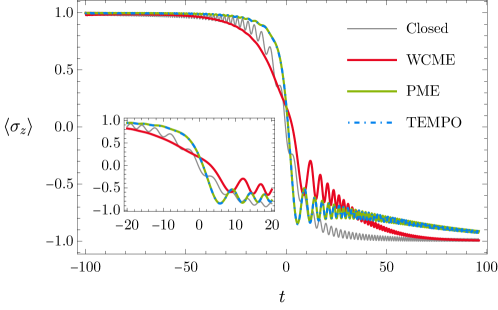
Figure 3: Population dynamics of the dissipative LZ model predicted by different dynamical models; closed unitary evolution, the weak-coupling master equation (WCME) (106), polaron master equation (PME) (94) and an exact numerical simulation provided by TEMPO. The inset shows the dynamics near to the avoided crossing. Parameters used: $\nu=0.1\Delta$, $t_{0}=-100/\Delta$, $t_{f}=100/\Delta$, $\alpha=0.4$, $\beta=1/\Delta$, $\omega_{c}=10\Delta$. The time axis is in units of $1/\Delta$.

Appendix C Benchmarking

Details of a simulation of the time-dependent LZ model to justify our choice of parameters used to compute the work statistics in Figure 1 and Figure 2 are provided here. We benchmark the reduced dynamics predicted by the PME (94) with numerically exact dynamics calculated with the TEMPO algorithm Strathearn et al. (2018); Gribben et al. (2022). In Figure 3 we show the population dynamics in the diabatic basis $\expectationvalue{\sigma_{z}}=\tr_{S}(\sigma_{z}\rho_{S}(t))=\tr_{S}(\sigma_{z}\rho_{PS}(t))$ with an initial state $\rho_{0}=\outerproduct{1}{1}$. We see excellent agreement between PME and TEMPO calculated dynamics, whilst the WCME (106) significantly overestimates the effect of the bath. For the tempo simulations, convergence was achieved with an singular value decomposition cutoff of $10^{-7}$, timestep of $\delta t=0.025$, and memory cutoff of $\tau_{c}=2$. Before starting the protocol, we allowed the bath to relax to a displaced thermal state, using a time window of $\tau_{W}=4$. This means that the protocol is initialised with the bath and system in a true equilibrium state of the system and environment.

References

- Jarzynski (2017) C. Jarzynski, Phys. Rev. X 7, 011008 (2017).
- Potočnik et al. (2018) A. Potočnik, A. Bargerbos, F. A. Schröder, S. A. Khan, M. C. Collodo, S. Gasparinetti, Y. Salathé, C. Creatore, C. Eichler, H. E. Türeci, et al., Nat. Comm. 9, 904 (2018).
- Maier et al. (2019) C. Maier, T. Brydges, P. Jurcevic, N. Trautmann, C. Hempel, B. Lanyon, P. Hauke, R. Blatt, and C. Roos, Phys. Rev. Lett. 122, 050501 (2019).
- Takahashi et al. (2020) H. Takahashi, E. Kassa, C. Christoforou, and M. Keller, Phys. Rev. Lett. 124, 013602 (2020).
- Ingold et al. (2008) G. Ingold, P. Hänggi, and P. Talkner, Phys. Rev. E 79, 061105 (2008).
- Strasberg et al. (2016) P. Strasberg, G. Schaller, N. Lambert, and T. Brandes, N. J. Phys 18, 073007 (2016).
- Perarnau-Llobet et al. (2018) M. Perarnau-Llobet, H. Wilming, A. Riera, R. Gallego, and J. Eisert, Phys. Rev. Lett. 120, 120602 (2018).
- Hsiang et al. (2018) J. T. Hsiang, C. H. Chou, Y. Subaşl, and B. L. Hu, Phys. Rev. E 97, 012135 (2018).
- Gelbwaser-Klimovsky and Aspuru-Guzik (2015) D. Gelbwaser-Klimovsky and A. Aspuru-Guzik, J. Phys. Chem.Lett. 6, 3477 (2015).
- Strasberg (2019) P. Strasberg, Phys. Rev. Lett. 123, 180604 (2019).
- Rivas (2020) Á. Rivas, Phys. Rev. Lett. 124, 160601 (2020).
- Talkner and Hänggi (2020) P. Talkner and P. Hänggi, Rev. Mod Phys. 92, 041002 (2020).
- Grabert et al. (1984) H. Grabert, U. Weiss, and P. Talkner, Z. Phys. B. 55, 87 (1984).
- Subasi et al. (2012) Y. Subasi, C. H. Fleming, J. M. Taylor, and B. L. Hu, Phys. Rev. E 86, 061132 (2012).
- Thingna et al. (2012) J. Thingna, J. S. Wang, and P. Hänggi, J. Chem. Phys 136, 194110 (2012).
- Cresser and Anders (2021) J. D. Cresser and J. Anders, Phys. Rev. Lett. 127, 250601 (2021).
- Trushechkin et al. (2022) A. S. Trushechkin, M. Merkli, J. D. Cresser, and J. Anders, AVS Quant. Sci. 4, 012301 (2022).
- Ford et al. (1985) G. W. Ford, J. T. Lewis, and R. F. O’Connell, Phys. Rev. Lett. 55, 2273 (1985).
- Jarzynski (2004) C. Jarzynski, J. Stat. Mech. 2004, P09005 (2004).
- Gelin and Thoss (2009) M. F. Gelin and M. Thoss, Phys. Rev. E 79, 051121 (2009).
- Philbin and Anders (2016) T. G. Philbin and J. Anders, J. Phys. A 49, 215303 (2016).
- Miller (2018) H. J. D. Miller, in Thermodynamics in the Quantum Regime: Fundamental Aspects and New Directions, Fundamental Theories of Physics, edited by F. Binder, L. A. Correa, C. Gogolin, J. Anders, and G. Adesso (Springer International Publishing, Cham, 2018) pp. 531–549.
- Campisi et al. (2009a) M. Campisi, P. Talkner, and P. Hänggi, Phys. Rev. Lett. 102, 210401 (2009a).
- Talkner et al. (2009) P. Talkner, M. Campisi, and P. Hänggi, J. Stat. Mech. Theory Exp. 2009, P02025 (2009).
- Campisi et al. (2009b) M. Campisi, P. Talkner, and P. Hänggi, J. Phys. A 42, 392002 (2009b).
- Schmidt et al. (2015) R. Schmidt, M. F. Carusela, J. P. Pekola, S. Suomela, and J. Ankerhold, Phys. Rev. B 91, 224303 (2015).
- Aurell (2017) E. Aurell, Entropy 19, 595 (2017).
- Funo and Quan (2018) K. Funo and H. T. Quan, Phys. Rev. Lett. 121, 40602 (2018).
- Makri and Makarov (1995) N. Makri and D. E. Makarov, J. Chem. Phys. 102, 4600 (1995).
- Strathearn et al. (2018) A. Strathearn, P. Kirton, D. Kilda, J. Keeling, and B. W. Lovett, Nat. Comm. 9, 3322 (2018).
- Cygorek et al. (2022) M. Cygorek, M. Cosacchi, A. Vagov, V. M. Axt, B. W. Lovett, J. Keeling, and E. M. Gauger, Nat. Phys. 18, 662 (2022).
- Nazir (2009) A. Nazir, Phys. Rev. Lett. 103, 146404 (2009).
- Jang et al. (2008) S. Jang, Y.-C. Cheng, D. R. Reichman, and J. D. Eaves, J. Chem. Phys. 129, 101104 (2008).
- McCutcheon and Nazir (2011) D. P. S. McCutcheon and A. Nazir, J. Chem. Phys 135, 114501 (2011).
- Kolli et al. (2011) A. Kolli, A. Nazir, and A. Olaya-Castro, J. Chem. Phys. 135, 154112 (2011).
- Jang (2011) S. Jang, J. Chem. Phys. 135, 34105 (2011).
- McCutcheon and Nazir (2010) D. P. McCutcheon and A. Nazir, N. J. Phys. 12, 113042 (2010).
- Wang et al. (2015) C. Wang, J. Ren, and J. Cao, Sci. Rep. 5, 11787 (2015).
- Popovic et al. (2021) M. Popovic, M. T. Mitchison, A. Strathearn, B. W. Lovett, J. Goold, and P. R. Eastham, PRX Quantum 2, 020338 (2021).
- Talkner et al. (2007) P. Talkner, E. Lutz, and P. Hänggi, Phys. Rev. E 75, 050102 (2007).
- Esposito et al. (2009) M. Esposito, U. Harbola, and S. Mukamel, Rev. Mod. Phys. 81, 1665 (2009).
- Silaev et al. (2014) M. Silaev, T. T. Heikkilä, and P. Virtanen, Phys. Rev. E 90, 22103 (2014).
- Suomela et al. (2015) S. Suomela, J. Salmilehto, I. G. Savenko, T. Ala-Nissila, and M. Möttönen, Phys. Rev. E 91, 22126 (2015).
- Liu and Xi (2016) F. Liu and J. Xi, Phys. Rev. E 94, 62133 (2016).
- Albash et al. (2012) T. Albash, S. Boixo, D. A. Lidar, and P. Zanardi, N. J. Phys 14, 123016 (2012).
- Yamaguchi et al. (2017) M. Yamaguchi, T. Yuge, and T. Ogawa, Phys. Rev. E 95, 012136 (2017).
- Mozgunov and Lidar (2020) E. Mozgunov and D. Lidar, Quantum 4, 227 (2020), 1908.01095 .
- Dai et al. (2022) X. Dai, R. Trappen, H. Chen, D. Melanson, M. A. Yurtalan, D. M. Tennant, A. J. Martinez, Y. Tang, E. Mozgunov, J. Gibson, J. A. Grover, S. M. Disseler, J. I. Basham, S. Novikov, R. Das, A. J. Melville, B. M. Niedzielski, C. F. Hirjibehedin, K. Serniak, S. J. Weber, J. L. Yoder, W. D. Oliver, K. M. Zick, D. A. Lidar, and A. Lupascu, (2022), arXiv:2207.02017 [quant-ph] .
- Chen and Lidar (2022) H. Chen and D. A. Lidar, Comm. Phys. 5, 112 (2022).
- Nazir and McCutcheon (2016) A. Nazir and D. P. S. McCutcheon, J. Phys. Cond. Matt. 28, 103002 (2016).
- Note (1) Both the weak coupling and polaron theory also show a peak at , however this is heavily suppressed when initialising the system in thermal equilibrium far from the anti-crossing.
- Newman et al. (2017) D. Newman, F. Mintert, and A. Nazir, Phys. Rev. E 95, 032139 (2017).
- Hekking and Pekola (2013) F. W. J. Hekking and J. P. Pekola, Phys. Rev. Lett. 111, 93602 (2013).
- Horowitz and Parrondo (2013) J. M. Horowitz and J. M. R. Parrondo, N. J. Phys 15, 085028 (2013).
- Gore et al. (2003) J. Gore, F. Ritort, and C. Bustamante, PNAS 100, 12564 (2003).
- Park et al. (2003) S. Park, F. Khalili-Araghi, E. Tajkhorshid, and K. Schulten, J. Chem. Phys. 119, 3559 (2003).
- Silbey and Harris (1984) R. Silbey and R. A. Harris, J. Chem. Phys. 80, 2615 (1984).
- Hsieh et al. (2019) C. Hsieh, J. Liu, C. Duan, and J. Cao, J. Phys. Chem. 123, 17196 (2019).
- Nazir and Schaller (2018) A. Nazir and G. Schaller, in Thermodynamics in the Quantum Regime: Fundamental Aspects and New Directions, Fundamental Theories of Physics, edited by F. Binder, L. A. Correa, C. Gogolin, J. Anders, and G. Adesso (Springer International Publishing, Cham, 2018) pp. 551–577.
- Liu (2018) F. Liu, Prog. Phys. 38, 1 (2018).
- Gribben et al. (2022) D. Gribben, D. M. Rouse, J. Iles-Smith, A. Strathearn, H. Maguire, P. Kirton, A. Nazir, E. M. Gauger, and B. W. Lovett, PRX Quantum 3, 010321 (2022).