Obtaining polynomial invariants for rooted trees from their random destruction

Abstract.

We use random destruction processes such as the random cutting model or site percolation on rooted trees to define several polynomial invariants for rooted trees. Some properties of these invariants are then exhibited, including recursion formulas and relations between them. The main result states that two of these invariants are complete, that is they distinguish rooted trees (in fact, even rooted forests) up to isomorphism. The proof method relies on recursion formulas and on irreducibility of the polynomials in suitable unique factorization domains. For other invariants, we provide counterexamples showing that they are not complete, although that question remains open for a certain trivariate invariant.

1. Introduction

The study of polynomial invariants in graph theory is of considerable tradition, with perhaps the best-known invariant being the Tutte polynomial [Tut47, Tut54]. For trees on $n$ vertices, it is well-known that the Tutte polynomial evaluates to $x^{n-1}$ and is thus of little use when investigating trees. To overcome this issue, Chaudhary, Gordon and McMahon in [GM89] and [CG91] defined specific Tutte polynomials for (rooted) trees by replacing the usual rank of a subgraph in the corank-nullity definition of the Tutte polynomial by different notions of tree rank. In these papers, several of the obtained (modified) Tutte polynomials introduced for rooted trees were shown to be complete invariants, that is, no two non-isomorphic rooted trees are assigned the same polynomial.

Since then, more complete polynomial invariants for rooted trees were found, such as polychromatic polynomials [BR00] and the rooted multivariable chromatic polynomial [LW22] – both invariants require a large number of variables. The bivariate Ising polynomial [AM09] and the Negami polynomial [NO96], originally defined for unrooted trees, were later shown to have versions for rooted trees that are complete invariants, see [Law11]. More recently, Liu [Liu21] found a complete bivariate polynomial as a generating function for a certain class of subtrees, and [RMW22] considers an extension of Liu’s polynomial to three variables.

In this paper, we define several polynomial invariants for rooted trees that come naturally out of random destruction processes on trees. Among these, two bivariate invariants are proven to be complete using an approach via irreducibility of polynomials and a suitable recursion, and for two more invariants examples are provided showing that they are not complete. Moreover, all polynomial invariants considered here are closely related, leading to several identities that might be interesting in their own right, or for the purpose of explicit computations relating to phenomena around the random cutting model or site percolation.

In Section 2, we fix notation and give a short explanation of the afore-mentioned random destruction processes, before we define the polynomial invariants in Section 3. Section 4 features several technical results like recursion identities for all polynomials. In Section 5 we formulate and prove the main theorem of the paper, Theorem 10. Finally, Section 6 contains several remarks, examples, and an open conjecture.

2. Preliminaries

Rooted trees and forests

For the purpose of this paper, a rooted tree $T$ is a finite tree with one distinguished vertex, called the root of $T$. It will be convenient to also consider rooted forests, by which we understand a finite (but possibly empty) disjoint union of rooted trees. By this convention, every component in a rooted forest is a rooted tree. A vertex is a leaf of a rooted forest if it has outdegree 0 (thus an isolated vertex is simultaneously a root and a leaf).

An isomorphism of rooted forests is a graph isomorphism that additionally maps roots to roots.

Given a rooted tree $T$, denote by $r$ the number of children of the root node $v_{0}$. We can construct a rooted forest from $T$ by removing $v_{0}$, thus creating a forest with $r$ components, and declaring the unique child of $v_{0}$ in each component to be the root node in that component. We will denote the resulting forest by $T-v_{0}$. The components of $T-v_{0}$ are also called the branches of $T$.

Conversely, given a rooted forest $F$ with $r\geq 0$ components, let $v_{0}$ be a vertex not in $F$ and draw an edge from $v_{0}$ to each of the $r$ roots in $F$. Upon declaring $v_{0}$ to be the root of the so-constructed tree, we have obtained a rooted tree. We will denote the resulting tree by $\wedge(F)$ or $\wedge(T_{1},\dots,T_{r})$ if $F$ is given by its components $T_{1},\dots,T_{r}$.

Since our definition allows for empty rooted forests (containing no vertices whatsoever), it follows immediately that $\wedge(F)-v_{0}\cong F$ and $\wedge(T-v_{0})\cong T$ for all rooted forests $F$ and all rooted trees $T$. In particular, removing the root of a tree and adding a joint root to a forest are inverse bijections between isomorphism classes of rooted trees and isomorphism classes of rooted forests.

For convenience, $\bullet$ will denote the rooted tree on one vertex.

Random destruction of trees

Two popular models for randomly destroying graphs are percolation and the cutting model. In $\mathsf{Ber}(q)$-site percolation, a probability $q\in[0,1]$ is fixed, and every vertex in a fixed underlying graph is deleted with probability $1-q$ and otherwise kept, independently from all other vertices. Percolation has been extensively studied, and we refer to [Gri99] as a general reference.

In the cutting model on a rooted tree $T$, vertices are deleted (i.e. cut) randomly one at a time, and all components not containing the root node are immediately discarded. This process necessarily stops once the root node is cut. Equivalently, one can equip each vertex $v$ in $T$ with an independent alarm clock ringing at a uniformly random time $X_{v}\in[0,1]$, at which the vertex $v$ is cut. It is easy to see that this continuous-time cutting model, as $t$ increases from 0 to 1, is exactly the evolution of the root cluster in the standard coupling of $\mathsf{Ber}(1-t)$-site percolation. The cutting model has first been considered by Meir and Moon in [MM70], but has received significant attention in the last two decades through works such as [Pan06, Jan06, Ber12, ABBH14], just to name a few.

For the cutting model on rooted trees, we say that separation occurs at the first time when the remaining tree does not contain any original leaf of $T$ anymore. The remaining tree at this point in time will be denoted by $T_{\mathfrak{S}}$ (cf. [Bur21]).

3. Setting the stage: Defining polynomials

Leaf-induced subforests

Let $F$ be a rooted forest. By a leaf-induced subforest $F^{\prime}$ we understand a rooted forest $F^{\prime}$ that is a (possibly empty) union of paths connecting roots of $F$ to leaves of $F$. In other words, any leaf of $F^{\prime}$ must also be a leaf of $F$. It follows that $F^{\prime}$ is completely determined by choosing a subset of the leaves of $F$, and connecting each of the chosen leaves to the root of its component. In particular, if $F$ has $\ell$ leaves, then it has $2^{\ell}$ leaf-induced subforests.

Definition 1.

For a rooted forest $F$, denote by $P_{F}(x,y)$ the bivariate generating function for leaf-induced subforests of $F$ according to their number of vertices and leaves. That is,

$$P_{F}(x,y)=\sum_{F^{\prime}\subseteq F\ \text{leaf-induced}}x^{|V(F^{\prime})|}y^{|L(F^{\prime})|},$$ (1)

where $V(F^{\prime})$ and $L(F^{\prime})$ denote the sets of vertices and leaves of $F^{\prime}$, respectively.

As an example, if $T$ is the path on $n$ vertices with the root situated on one end, then $P_{T}(x,y)=1+x^{n}y$, since the only leaf-induced subforests are the empty one and $T$ itself. For $T$ being the star on $n+1$ vertices, with the root being the central vertex, we have $P_{T}(x,y)=1+\sum_{k=1}^{n}\binom{n}{k}x^{k+1}y^{k}$, which can be seen directly from a combinatorial argument, or computed recursively as will be established in the next section.

For a rooted tree $T$, the connection between $P_{T}$ and continuous-time cuttings on $T$ comes from the specialization to $y=-1$; indeed, Propositions 18 and 21 in [Bur21] together state that

$$p_{T}(q):=1-P_{T}(q,-1)$$ (2)

for $q\in[0,1]$ equals the probability $\mathsf{Ber}(q)$-site percolation contains a path from the root to a leaf. (Equivalently, it is the probability that separation has not occurred by time $1-q$ in the continuous-time cutting model). This connection makes $p_{T}(q)$ useful for several other computations as well, which is why it reappears in other contexts in this paper. Moreover, $p_{T}(q)$ was also investigated in [Dev11, CCDT13] in the context of transversals in trees. Finally, Propositions 2.16 and 2.17 and the comment thereafter in [RMW22] establish a connection between the trivariate polynomial considered there, and $P_{T}$.

Admissible subtrees

By a subtree of a rooted tree $T$ we mean either the empty subgraph of $T$ or any connected subgraph of $T$ that contains the root (though we will break with this convention in the context of fringe subtrees which generally do not contain the root node of $T$, see the paragraph above Definition 4). A subgraph $T_{*}$ of a rooted tree $T$ is called admissible if $\mathbf{P}[T_{\mathfrak{S}}=T_{*}]>0$. It is easy to see that a non-empty connected subgraph $T_{*}$ is admissible if and only if it contains the root of $T$, but none of the leaves of $T$. The empty subtree is always admissible, as a consequence of the definition. We write $\mathscr{A}(T)$ for the set of all admissible subgraphs of $T$.

Since a subtree $T^{\prime}$ of $T$ is uniquely determined by its vertex set, we will not distinguish between $T^{\prime}$ and its vertex set.

Given a set $S$ of vertices in a rooted tree $T$, we denote by $\partial S$ the boundary of $S$, i.e. the set of all vertices that are adjacent to $S$ but not themselves in $S$. For our purposes, it is convenient to define $\partial\emptyset=\{\text{root}\}$.

Definition 2.

For a rooted tree $T$, denote by $S_{T}(x,y)$ (resp. $A_{T}(x,y)$) the bivariate generating function for subtrees (resp. admissible subtrees) of $T$ according to their number of vertices and boundary vertices. That is,

$$S_{T}(x,y)=\sum_{T^{\prime}\subseteq T}x^{|T^{\prime}|}y^{|\partial T^{\prime}|}$$ (3)

and

$$A_{T}(x,y)=\sum_{T^{\prime}\in\mathscr{A}(T)}x^{|T^{\prime}|}y^{|\partial T^{\prime}|}.$$ (4)

For example, if $T$ is the path on $n$ vertices, again with the root located at one of the endpoints, then any shorter path starting at the root is a non-empty admissible subtree, and thus $A_{T}(x,y)=y(1+x+\dots+x^{n-1})$. Additionally, the entire path itself is the only non-admissible subtree (with $n$ vertices and empty boundary), so $S_{T}(x,y)=A_{T}(x,y)+x^{n}$. On the other hand, for $T$ being the centrally-rooted star on $n+1$ vertices, we have only two admissible subtrees and obtain $A_{T}(x,y)=y+xy^{n}$, but $S_{T}(x,y)=y+x(x+y)^{n}$.

In the setting of $\mathsf{Ber}(q)$-site percolation on a rooted tree $T$, the term $q^{|T^{\prime}|}(1-q)^{|\partial T^{\prime}|}$ gives the probability that a subgraph $T^{\prime}$ of $T$ is the root cluster of the percolation. The restriction to admissible subgraphs in (4) will lead to connections between $A_{T}$ and the polynomials $p_{T}$ and $M_{T}$, see Lemma 9 below.

Remark 3.

We can extend Definition 2 to rooted forests, as follows: If $F$ is a rooted forest having components $T_{1},\dots,T_{r}$, then define

$$S_{F}(x,y):=\prod_{i=1}^{r}S_{T_{i}}(x,y)\qquad\text{ and }\qquad A_{F}(x,y):=\prod_{i=1}^{r}A_{T_{i}}(x,y).$$ (5)

It is still possible to relate these polynomials to the random destruction of rooted forests in a matter analogous to the case of trees, but we will omit the details here.

The graph at separation

The fringe subtree $T_{v}$ of a rooted tree $T$ is the induced subgraph of $T$ consisting of the vertex $v$ (which is designated the root of $T_{v}$) and all descendants of $v$. The following definition is motivated by its connection to equation (7), which will be discussed below.

Definition 4.

For a rooted tree $T$, denote by $M_{T}(x,y,z)$ the trivariate polynomial defined by

$$M_{T}(x,y,z)=\sum_{T^{\prime}\in\mathscr{A}(T)}x^{|T^{\prime}|}y^{|\partial T^{\prime}|-1}\sum_{v\in\partial T^{\prime}}\frac{1}{z}p_{v}(z),$$ (6)

where $p_{v}(z):=p_{T_{v}}(z)=1-P_{T_{v}}(z,-1)$.

It follows from either Lemma 5 below or from the probabilistic interpretation of $p_{v}$ that $p_{v}(0)=0$, so $\frac{1}{z}p_{v}(z)$ is indeed a polynomial in $z$.

Assume that the continuous-time cutting model separates $T$ at some time $q_{0}\in[0,1]$, and leaves behind an admissible graph $T^{\prime}$. Then immediately before separation, all but one of the vertices in $\partial T^{\prime}$ must have been cut already, with the exceptional vertex $v\in\partial T^{\prime}$ being such that there still is a path connecting the root to a leaf through $v$ present. Moreover, none of the vertices in $T^{\prime}$ can have been cut before $q_{0}$. In particular, at time $q_{0}$, the fringe subtree $T_{v}$ has not yet been separated itself. Employing this idea, it is possible to show that

$$\mathbf{P}[T_{\mathfrak{S}}=T^{\prime}]=\int_{0}^{1}u^{|T^{\prime}|-1}(1-u)^{|\partial T^{\prime}|-1}\sum_{v\in\partial T^{\prime}}p_{v}(u)\,\,\textnormal{d}u$$

(cf. Proposition 13 in [Bur21]). From this, it follows immediately that the probability generating function of $|T_{\mathfrak{S}}|$ is given by

$$\sum_{n\geq 0}\mathbf{P}[|T_{\mathfrak{S}}|=n]x^{n}=\int_{0}^{1}M_{T}(xu,1-u,u)\,\,\textnormal{d}u$$ (7)

It might therefore seem more useful to directly investigate the polynomial on the right-hand side of (7); however, a possible advantage of $M_{T}$ lies in the recursion (13).

4. Some identities

The purpose of this section is to exhibit recursion formulas for all relevant polynomials, as well as identities relating the polynomials to one another. The following first lemma will prove useful throughout:

Lemma 5.

Let $F$ be a rooted forest. Then:

1. The number of vertices of $F$ equals $\deg_{x}(P_{F})$.

2. The number $\ell$ of leaves of $F$ equals $\deg_{y}(P_{F})$.

3. Specializing to $x=1$ gives $P_{F}(1,y)=(1+y)^{\ell}$. In particular, we have $P_{F}(1,-1)=0$ unless $F$ is the empty forest, in which case $P_{F}\equiv 1$.

Proof.

Parts (a) and (b) are immediate from Definition 1. For part (c), note that $P_{F}(1,y)$ is the generating function for leaf-induced subforests with a given number of leaves. Since subsets of leaves are in bijection with leaf-induced subforests, we have $P_{F}(1,y)=\sum_{k=0}^{\ell}\binom{\ell}{k}y^{k}=(1+y)^{\ell}$. ∎

Lemma 6.

We have $P_{\bullet}(x,y)=1+xy$ and $p_{\bullet}(x)=x$. Let $F$ be a non-empty rooted forest with rooted trees $T_{1},\dots,T_{r}$ ($r\geq 1$) as its components.

1. We then have

   $$P_{F}(x,y)=\prod_{i=1}^{r}P_{T_{i}}(x,y).$$ (8)

2. For $T=\wedge(F)$, that is, for a tree having branches $T_{1},\dots,T_{r}$, we have

   $$P_{T}(x,y)=1-x+xP_{F}(x,y).$$ (9)

3. As a consequence,

   $$p_{T}(x)=x\left(1-\prod_{i=1}^{r}(1-p_{T_{i}}(x))\right).$$ (10)

Proof.

For part (a), let $F^{\prime}$ be any leaf-induced subforest of $F$. Then the intersections $F^{\prime}\cap T_{1},\dots,F^{\prime}\cap T_{r}$ are (possibly empty) leaf-induced subtrees of $T_{1},\dots,T_{r}$, respectively. In this way, we can identify $F^{\prime}$ with the $r$-tuple $(F^{\prime}\cap T_{1},\dots,F^{\prime}\cap T_{r})$, and both the number of vertices and the number of leaves in these components add up to the respective numbers of $F^{\prime}$. Thus the bivariate generating function $P_{F}$ equals the product $\prod_{i=1}^{r}P_{T_{i}}$.

For part (b), observe that there is a bijection between non-empty leaf-induced subforests of $F$ and leaf-induced subtrees of $\wedge(F)$, simply by adding the root node of $\wedge(F)$ to the subforest of $F$. Since this increases the number of vertices by 1, the generating function for those subtrees is given by $x\left(P_{F}(x,y)-1\right)$. Accounting for the empty subforest of $\wedge(F)$ as well yields the result.

Finally, part (c) follows from (a) and (b) after recalling the definition $p_{T}(x)=1-P_{T}(x,-1)$. ∎

Lemma 7.

We have $S_{\bullet}(x,y)=y+x$ and $A_{\bullet}(x,y)=y$. If $T$ is a rooted tree with branches $T_{1},\dots,T_{r}$, then

$$S_{T}(x,y)=y+x\prod_{i=1}^{r}S_{T_{i}}(x,y)$$ (11)

and

$$A_{T}(x,y)=y+x\prod_{i=1}^{r}A_{T_{i}}(x,y).$$ (12)

Proof.

The claims for the tree on one vertex are easily verified from the definitions.

Consider a subtree $T^{\prime}$ of $T$. Then $T^{\prime}$ is either empty, or it consists of the root together with the parts belonging to individual branches, $T_{i}^{\prime}=T^{\prime}\cap T_{i}$, for $i=1,\dots,r$. In the non-empty case, $T^{\prime}$ is uniquely determined by the $T_{i}^{\prime}$, and we have $|T^{\prime}|=1+\sum_{i}|T^{\prime}_{i}|$ and $|\partial T^{\prime}|=\sum_{i}|\partial T^{\prime}_{i}|$. Thus,

$$S_{T}(x,y) =\sum_{T^{\prime}\subseteq T}x^{|T^{\prime}|}y^{|\partial T^{\prime}|}=y+x\!\!\sum_{T^{\prime}_{1}\subseteq T_{1}}\!\!\cdots\!\!\sum_{T^{\prime}_{r}\subseteq T_{r}}\!\!x^{\sum_{\ell}|T^{\prime}_{\ell}|}y^{\sum_{\ell}|\partial T^{\prime}_{\ell}|}$$

$$=y+x\prod_{i=1}^{r}\sum_{T^{\prime}_{i}\subseteq T_{i}}x^{|T^{\prime}_{i}|}y^{|\partial T^{\prime}_{i}|}=y+x\prod_{i=1}^{r}S_{T_{i}}(x,y),$$

which proves (11).

Note that if $T^{\prime}$ is an admissible subtree of $T$, then the corresponding $T^{\prime}_{i}$ will be admissible subtrees of $T_{i}$, for each $i$. Conversely, any non-empty $T^{\prime}$ is again uniquely determined by the $T^{\prime}_{i}$. Hence, the computations for equation (12) are identical to the ones above. ∎

Lemma 8.

We have $M_{\bullet}(x,y,z)=1$. If $T$ is a rooted tree with branches $T_{1},\dots,T_{r}$ then

$$M_{T}(x,y,z)=\frac{1}{z}p_{T}(z)+x\sum_{i=1}^{r}M_{T_{i}}(x,y,z)\prod_{j\neq i}A_{T_{j}}(x,y)$$ (13)

Proof.

We use the same approach and notation as in the proof of Lemma 7. So, any $T^{\prime}\in\mathscr{A}(T)$ is either empty, or contains the root together with parts $T_{i}^{\prime}\in\mathscr{A}(T_{i})$ for each branch $T_{1},\dots,T_{r}$. Thus, we obtain

$$M {}_{T}(x,y,z)=\sum_{T^{\prime}\in\mathscr{A}(T)}x^{|T^{\prime}|}y^{|\partial T^{\prime}|-1}\sum_{v\in\partial T^{\prime}}\frac{p_{v}(z)}{z}$$

$$=\frac{p_{T}(z)}{z}+\!\!\sum_{T^{\prime}_{1}\in\mathscr{A}(T_{1})}\!\!\cdots\!\!\sum_{T^{\prime}_{r}\in\mathscr{A}(T_{r})}\!\!x^{1+\sum_{\ell}|T^{\prime}_{\ell}|}y^{\sum_{\ell}\partial|T^{\prime}_{\ell}|-1}\!\sum_{v\in\bigcup_{i}\partial T^{\prime}_{i}}\frac{p_{v}(z)}{z}$$

$$=\frac{p_{T}(z)}{z}+\frac{x}{yz}\sum_{i=1}^{r}\sum_{T^{\prime}_{1}\in\mathscr{A}(T_{1})}\!\!\cdots\!\!\sum_{T^{\prime}_{r}\in\mathscr{A}(T_{r})}\!\!x^{\sum_{\ell}|T^{\prime}_{\ell}|}y^{\sum_{\ell}\partial|T^{\prime}_{\ell}|}\sum_{v\in\partial T^{\prime}_{i}}p_{v}(z)$$

$$=\frac{p_{T}(z)}{z}+\frac{x}{yz}\sum_{i=1}^{r}\left(\prod_{j\neq i}\sum_{T^{\prime}_{j}\in\mathscr{A}(T_{j})}\!\!\!x^{|T^{\prime}_{j}|}y^{|\partial T^{\prime}_{j}|}\right)\!\!\sum_{T^{\prime}_{i}\in\mathscr{A}(T_{i})}\!\!\!x^{|T^{\prime}_{i}|}y^{|\partial T^{\prime}_{i}|}\sum_{v\in\partial T^{\prime}_{i}}p_{v}(z).$$

By comparing the final expression to Definitions 2 and 4, we obtain (13). ∎

Lemma 9.

For any rooted tree $T$, we have the following three identities:

$$M_{T}(x,y,1)=\frac{\partial}{\partial y}A_{T}(x,y)$$ (14)

$$A_{T}(x,1-x)=1-p_{T}(x)$$ (15)

$$M_{T}(x,1-x,x)=\frac{\,\textnormal{d}}{\,\textnormal{d}x}p_{T}(x).$$ (16)

Proof.

For the proof of (14), consider a vertex $v\in V(T)$. Then $p_{v}(1)=1-P_{T_{v}}(1,-1)=1$ by Lemma 5(c), and we thus have

$$x^{|T^{\prime}|}y^{|\partial T^{\prime}|-1}\sum_{v\in\partial T^{\prime}}\left.\frac{p_{v}(z)}{z}\right|_{z=1}=|\partial T^{\prime}|x^{|T^{\prime}|}y^{|\partial T^{\prime}|-1}$$

for any fixed $T^{\prime}\in\mathscr{A}(T)$. Hence

$$M_{T}(x,y,1)=\sum_{T^{\prime}\in\mathscr{A}(T)}|\partial T^{\prime}|x^{|T^{\prime}|}y^{|\partial T^{\prime}|-1}=\frac{\partial}{\partial y}A_{T}(x,y),$$

as required.

The identity (15) follows immediately from comparing the recursions (12) and (10).

Equality (16) is trivially true for $T=\bullet$, and we will now use an inductive argument: Assuming that the identity holds for any trees $T_{1},\dots,T_{r}$, we will show that it is also true for $T=\wedge(T_{1},\dots,T_{r})$. To do this, consider the recursion (10) and take the derivative:

$$\frac{\,\textnormal{d}p_{T}(x)}{\,\textnormal{d}x} =1-\prod_{i=1}^{r}(1-p_{T_{i}}(x))+x\sum_{i=1}^{r}\frac{\,\textnormal{d}p_{T_{i}}(x)}{\,\textnormal{d}x}\prod_{j\neq i}(1-p_{T_{j}}(x))$$

$$=\frac{p_{T}(x)}{x}+x\sum_{i=1}^{r}M_{T_{i}}(x,1-x,x)\prod_{j\neq i}A_{T_{j}}(x,1-x)$$

$$=M_{T}(x,1-x,x).$$

For the second equality, we used (10), (15), and the induction hypothesis, and the final equality follows from the recursion for $M$, (13). ∎

Observe that by (14), $A_{T}$ is uniquely determined by $M_{T}$, since $\eqref{eq:Arec}$ implies that $A_{T}(x,0)=0$. Moreover, $p_{T}$ is uniquely determined by $A_{T}$ according to (15).

5. Two complete invariants

As an immediate consequence of Definitions 1,2, and 4, we get that two isomorphic rooted trees $T_{1}\cong T_{2}$ have the same polynomials. The aim of this section is to show that the converse is true as well for the polynomials $P$ and $S$. Specifically, we will prove the following theorem:

Theorem 10.

The polynomials $P$ and $S$ as defined in Definition 1 and Remark 3 are complete invariants for rooted forests. In other words, for rooted forests $F_{1},F_{2}$ we have $P_{F_{1}}=P_{F_{2}}$ or $S_{F_{1}}=S_{F_{2}}$ if and only if $F_{1}\cong F_{2}$.

As pointed out above, it only remains to show that either of the two equalities is sufficient for $F_{1}\cong F_{2}$, and we devote the rest of the section to this proof.

A key ingredient for the proof will be that in a unique factorization domain (UFD), polynomials can – by definition – be factored uniquely into irreducibles; and we will employ the fact that both $\mathbb{Z}[x,y]$ and $\mathbb{C}[x,y]$ are UFDs.

By the stem of a rooted tree, we understand the set of vertices constructed in the following iterative way: Start by including the root node of $T$. If the last included vertex has a unique child, include that child as well. Otherwise stop. In other words, the stem consists of all those vertices between the root and the first “branching” of the tree (the two endpoints included). For convenience, we declare the stem of a rooted forest on zero or at least two components to be the empty set.

Lemma 11.

Let $F$ be a rooted forest. Then, the number $s$ of vertices in the stem of $F$ equals $p^{\prime}_{F}(1)=-\left.\frac{\partial P_{F}}{\partial x}\right|_{(1,-1)}$, with the partial derivative being zero if $F$ is not a tree.

Proof.

The claim is obviously true for the empty rooted forest. In all other cases, we use induction on $s$, beginning with $s=0$ (i.e. $F$ has at least two components).

For $s=0$, denote by $T_{1},\dots,T_{r}$ for $r\geq 2$ the components of $F$. Then $P_{T_{i}}(1,-1)=0$ for all $i=1,\dots,r$ by Lemma 5(c), so the polynomial

$$P_{F}(x,-1)=\prod_{i=1}^{r}P_{T_{i}}(x,-1)$$

has an $r$-fold zero at $x=1$. In particular, $\left.\frac{\partial P_{F}}{\partial x}\right|_{(1,-1)}=0$.

Assume that we have already shown the statement for some $s\geq 0$. Let $F$ be any rooted tree with $s+1$ vertices in its stem. Then $F=\wedge(F^{\prime})$ where $F^{\prime}$ is the forest obtained by removing the root of $F$, and $F^{\prime}$ is a rooted forest with $s$ stem vertices. In the special case where $F^{\prime}$ is the empty forest, $F$ is the rooted tree on a single vertex, and we can check directly that $-\left.\frac{\partial(1+xy)}{\partial x}\right|_{(1,-1)}=1$. In any other case, we employ Lemma 6(b) and the induction hypothesis to obtain

$$\left.\frac{\partial P_{F}}{\partial x}\right|_{(1,-1)}=-1+P_{F^{\prime}}(1,-1)+\left.\frac{\partial P_{F^{\prime}}}{\partial x}\right|_{(1,-1)}=-1-s,$$

since $P_{F^{\prime}}(1,-1)=0$. ∎

Proposition 12.

Let $F$ be a non-empty rooted forest. Then, $P_{F}$ is irreducible in $\mathbb{C}[x,y]$ if and only if $F$ is a tree.

Proof.

If $F$ is not a tree, then it consists of at least 2 components, each containing at least one vertex. Thus by part (a) in Lemma 6, $P_{F}$ factors into non-constant polynomials.

Now assume that $F$ is a tree on $n\geq 1$ vertices with $s\geq 1$ vertices in its stem, having $\ell\geq 1$ leaves. Assume $P_{F}=fg$ for $f,g\in\mathbb{C}[x,y]$. Specializing to $x=1$, we obtain $f(1,y)=(1+y)^{k_{1}}$ and $g(1,y)=(1+y)^{k_{2}}$ for $k_{1},k_{2}\geq 0$ with $k_{1}+k_{2}=\ell$, according to Lemma 5(c) and because the factors $1+y$ are irreducible. If both $k_{1},k_{2}>0$ then the product rule dictates

$$-s=\left.\frac{\partial P_{F}}{\partial x}\right|_{(1,-1)}=f(1,-1)\cdot\left.\frac{\partial g}{\partial x}\right|_{(1,-1)}+g(1,-1)\cdot\left.\frac{\partial f}{\partial x}\right|_{(1,-1)}=0,$$

a contradiction. Hence, without loss of generality $k_{1}=0,k_{2}=\ell$, and so $\deg_{y}(P_{F})=\ell=\deg_{y}(g)$, which implies $\deg_{y}(f)=0$. In other words, $f$ can be considered a univariate polynomial in $x$.

Now write

$$P_{F}(x,y)=a_{\ell}(x)y^{\ell}+\dots+a_{1}(x)y+a_{0}(x)$$

for suitable polynomials $a_{0},a_{1},\dots,a_{\ell}\in\mathbb{C}[x]$. If $f(x)$ is a divisor of $P_{F}$, it must therefore be a common divisor of $a_{0},\dots,a_{\ell}$. However, from Definition 1 we infer that $a_{0}(x)=1$. Thus $f(x)$ is a constant. ∎

Proposition 13.

Let $F$ be a non-empty rooted forest. Then $S_{F}$ is irreducible in $\mathbb{Z}[x,y]$ if and only if $F$ is a tree.

Proof.

If $F$ is not a tree, the reducibility of $S_{F}$ follows from the definition in Remark 3.

To show irreducibility in the case where $F$ is a rooted tree, we use Eisenstein’s criterion on the integral domain $\mathfrak{D}:=\mathbb{Z}[y]$. Since $\mathbb{Z}[x,y]\cong\mathfrak{D}[x]$, we can consider the prime ideal $\mathfrak{p}=\langle y\rangle$ in $\mathfrak{D}$. Writing $S_{F}$ as

$$S_{F}(x,y)=a_{0}(y)+a_{1}(y)x+\dots+a_{n}(y)x^{n}$$ (17)

with $a_{0},a_{1},\dots,a_{n}\in\mathfrak{D}$, we note that $a_{n}=1$ since the highest $x$-degree term in $S_{F}$ stems from the subgraph that is the entire tree, which contains $n=|V(F)|$ vertices, and no boundary vertices. Hence $a_{n}\notin\mathfrak{p}$. Moreover, any smaller subtree $T^{\prime}\subseteq F$ omits a vertex in $F$, and therefore has a vertex adjacent to, but not in $T^{\prime}$ (in the special case where $T^{\prime}=\emptyset$, this vertex is the root of $F$). Thus, the strict subtrees all contribute monomials divisible by $y$, and hence $a_{0},\dots,a_{n-1}\in\mathfrak{p}$. Finally, for $T^{\prime}=\emptyset$ we have $\partial T^{\prime}=\{\textnormal{root}\}$, thus $a_{0}(y)=y\notin\mathfrak{p}^{2}$ (and this is only correct if $F$ is a tree). Therefore $S_{F}$ cannot be factored into non-constant polynomials in $\mathfrak{D}[x]$ according to Eisenstein’s criterion, and since $a_{n}=1$ it is even irreducible in $\mathbb{Z}[x,y]$. ∎

We now have all the tools assembled to prove Theorem 10.

Proof of Theorem 10.

Assume first $P_{F_{1}}=P_{F_{2}}$. Since the polynomial determines the number of vertices and the number of vertices in the stem, those characteristics of $F_{1}$ and $F_{2}$ coincide, and we denote them by $n$ and $s$, respectively, as in the proof of Proposition 12.

Suppose the claim is false. Then there exist non-isomorphic $F_{1},F_{2}$ with $P_{F_{1}}=P_{F_{2}}$, and we can consider such a pair with $n$ minimal. If $s\geq 1$, then $F_{i}$ is a tree with root $\rho_{i}$ (for $i=1,2$), and we can consider $F_{1}-\rho_{1}$ and $F_{2}-\rho_{2}$ instead. As noted in the previous section, we have $F_{i}\cong\wedge(F_{i}-\rho_{i})$ for $i=1,2$, so by Lemma 6(b) we obtain $P_{F_{1}-\rho_{1}}=P_{F_{2}-\rho_{2}}$. By the minimality of $F_{1},F_{2}$, it follows that $F_{1}-\rho_{1}\cong F_{2}-\rho_{2}$, and hence $F_{1}\cong F_{2}$, a contradiction. Therefore, the minimal counterexamples $F_{1},F_{2}$ have to be either empty (which is trivially not a counterexample) or forests with at least 2 components each.

So, denote by $T_{1},\dots,T_{r}$ and $T^{\prime}_{1},\dots,T^{\prime}_{r^{\prime}}$ the components of $F_{1}$ and $F_{2}$, respectively. Lemma 6 yields

$$\prod_{i=1}^{r}P_{T_{i}}=P_{F_{1}}=P_{F_{2}}=\prod_{j=1}^{r^{\prime}}P_{T^{\prime}_{j}}.$$

As we are working in the UFD $\mathbb{C}[x,y]$ and the factors $P_{T_{i}}$ and $P_{T^{\prime}_{j}}$ are monic irreducibles by Proposition 12, it follows that $r=r^{\prime}$ and that there is a permutation $\pi\in S_{r}$ with $P_{T_{i}}=P_{T^{\prime}_{\pi(i)}}$ for $i=1,\dots,r$. Invoking again the minimality of $F_{1},F_{2}$, we conclude $T_{i}\cong T^{\prime}_{\pi(i)}$, and these isomorphisms can be glued together to an isomorphism $F_{1}\cong F_{2}$, which is the desired contradiction.

Assume now $S_{F_{1}}=S_{F_{2}}$ instead. Observe that $S$ again determines the number of vertices, $n$ and the number of vertices in the stem, $s$. Indeed, $n$ is given as the $x$-degree, and $s=\max(j,n)$, where $j$ is the lowest index such that $\deg_{y}a_{j}(y)>1$ when we represent $S$ as in equation (17) (this is because the last vertex in the stem is the closest vertex to the root that has more than one descendant, so the subtree induced by the stem is the smallest subtree to have a boundary with more than one vertex, unless $s=n$). Observe moreover that for a rooted tree $T$, we have $S_{T-\textnormal{root}}=\frac{1}{x}(S_{T}-y)$, which follows from comparing the recursion (11) with (5).

With these observations in place, the rest of the argument works entirely analogously to the previous case, except that we work in the UFD $\mathbb{Z}[x,y]$ (rather than $\mathbb{C}[x,y]$), due to Proposition 13. ∎

6. Remarks, examples, and open problems

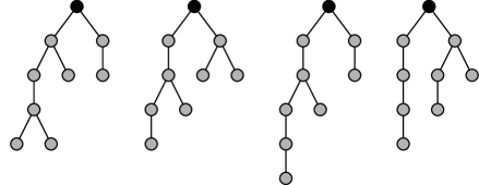
Figure 1. Non-isomorphic rooted trees $T_{1},T_{2},T_{3},T_{4}$ (from left to right).

Remark 14.

Unlike $P$, the univariate polynomial $p$ is not a complete invariant for rooted trees: As S. Wagner pointed out (​​[Wag]), the trees $T_{1},T_{2}$ and $T_{3},T_{4}$ in Figure 1 form two pairs of non-isomorphic trees that share the same polynomial, namely

$$p_{T_{1}}(x)=p_{T_{2}}(x) =2x^{3}+x^{5}-3x^{6}-x^{7}+3x^{8}-x^{9},\ \text{and}$$

$$p_{T_{3}}(x)=p_{T_{4}}(x) =x^{3}+x^{4}-x^{7}-x^{8}+x^{9}.$$

In fact, it can be verified by a computer search that these are the smallest such pairs. To exemplify Theorem 10, the corresponding bivariate polynomials are given by

$$P_{T_{1}} =2x^{3}y+2x^{5}y+x^{5}y^{2}+3x^{6}y^{2}+2x^{7}y^{2}+x^{7}y^{3}+3x^{8}y^{3}+x^{9}y^{4}$$

$$P_{T_{2}} =2x^{3}y+x^{4}y+x^{4}y^{2}+x^{5}y+3x^{6}y^{2}+2x^{7}y^{2}+x^{7}y^{3}+3x^{8}y^{3}+x^{9}y^{4}$$

$$P_{T_{3}} =x^{3}y+x^{4}y+x^{6}y+x^{6}y^{2}+x^{7}y^{2}+x^{8}y^{2}+x^{9}y^{3}$$

$$P_{T_{4}} =x^{3}y+x^{4}y+x^{5}y+x^{5}y^{2}+x^{7}y^{2}+x^{8}y^{2}+x^{9}y^{3},$$

which are pairwise different.

Remark 15.

Lemma 9 implies that $M$ is a stronger invariant (in the sense that it distinguishes more trees) than $A$, and $A$ is a stronger invariant than $p$. In fact, these relations are strict: The trees $T_{3}$ and $T_{4}$ from Figure 1 are distinguished by $A$ but not by $p$, and the trees $T_{1}$ and $T_{2}$ are distinguished by $M$ but not by $A$. Indeed, we have

$$A_{T_{1}} =A_{T_{2}}=y+xy^{2}+x^{2}y^{2}+x^{2}y^{3}+2x^{3}y^{3}+x^{4}y^{3}+x^{4}y^{4}+x^{5}y^{4}$$

$$A_{T_{3}} =y+xy^{2}+2x^{2}y^{2}+x^{3}y^{2}+x^{3}y^{3}+2x^{4}y^{3}+2x^{5}y^{3}+x^{6}y^{3}$$

$$A_{T_{4}} =y+xy^{2}+x^{2}y^{2}+x^{2}y^{3}+x^{3}y^{2}+2x^{3}y^{3}+x^{4}y^{2}+2x^{4}y^{3}+2x^{5}y^{3}+x^{6}y^{3}$$

and

$$M_{T_{1}} =\frac{p_{T_{1}}(z)}{z}+xy(2z+2z^{3}-3z^{4}+z^{5})+x^{2}y(1+z+2z^{3}-3z^{4}+z^{5})$$

$$\quad+x^{2}y^{2}(1+z+2z^{2}-z^{3})+2x^{3}y^{2}(3+3z+z^{2}-z^{3})$$

$$\quad+x^{4}y^{2}(2+2z-z^{2})+x^{4}y^{3}(3+z)+4x^{5}y^{3}$$

$$M_{T_{2}} =\frac{p_{T_{2}}(z)}{z}+xy(2z+z^{3}-z^{4})+x^{2}y(3z-z^{3})+x^{2}y^{2}(2+z^{2}+z^{3}-z^{4})$$

$$\quad+2x^{3}y^{2}(3+4z-z^{3})+x^{4}y^{2}(2+2z-z^{2})+x^{4}y^{3}(3+z)+4x^{5}y^{3}.$$

In light of these examples, it is worth noting that it is possible to fully describe all trees with 3 leaves that share the same $p_{T}$ with a different tree. In fact, they are of the structure depicted in Figure 2 (but we omit the proof in the interest of brevity). It is then easy to see that these trees will always be distinguished by $A$, since $T$ has an admissible subgraph with $s+3k-\beta-2$ vertices, and 2 boundary vertices; whereas the largest admissible subgraph in $\tilde{T}$ with 2 boundary vertices contains only $s+3k-2\beta-2$ vertices, hence $\deg_{x}[y^{2}]A_{T}>\deg_{x}[y^{2}]A_{\tilde{T}}$.

In full generality, it appears to be a difficult problem to give a graph-theoretic description for the rooted trees $T$ that have a “cousin” $T^{\prime}$ such that $p_{T}=p_{T^{\prime}}$ (or $A_{T}=A_{T^{\prime}}$).

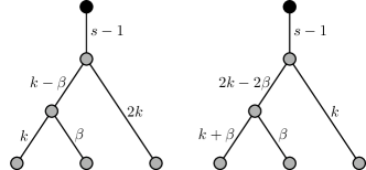
Figure 2. The structure of non-isomorphic rooted trees $T$ (left) and $\tilde{T}$ (right) with 3 leaves with $p_{T}(x)=p_{\tilde{T}}(x)=x^{s}(x^{k}+x^{2k-\beta}-x^{3k}-x^{4k-\beta}+x^{4k})$. An edge labelled by $x$ indicates a path on $x$ edges. Here, $s$ denotes the number of vertices in the stem, $k\geq 2$, and $\beta\in\{1,\dots,k-1\}$.

Remark 16.

It is worth emphasizing that despite satisfying the same recursion formula – compare (11) and (12) – and only differing in their initial values, the polynomial $S$ is a complete invariant, whereas the polynomial $A$ is not. In particular, it follows from the proof of Theorem 10 that $A_{T}$ is reducible for some trees $T$. This is obvious at first glance, since $y$ is a divisor of $A_{T}$ for every $T$, but this cannot be the only obstacle since otherwise $\frac{1}{y}A$ could be a complete invariant, and therefore also $A$. Indeed, the branches of the trees $T_{1}$ and $T_{2}$ from the previous remarks have a more interesting factorization, namely

$$y(1+xy)(1+x^{2}y)\quad\text{ and }\quad y(1+x)$$

for the two branches of $T_{1}$, and

$$y(1+x)(1+x^{2}y)\quad\text{ and }\quad y(1+xy)$$

for the two branches of $T_{2}$.

Remark 17.

Theorem 3.2 in [Liu21] gives a method to obtain a complete invariant for unrooted trees from a complete polynomial invariant for rooted trees that is irreducible in a suitable polynomial ring. The idea is to replace the unrooted tree by a rooted forest that determines the tree up to isomorphism, and then assign to the forest the product of the polynomials of its connected components. While the same idea works for the polynomials of Theorem 10, we prefer to formulate the statement in terms of complete invariants for rooted trees instead.

Conjecture 18.

The polynomial $M$ defines a complete invariant for rooted trees.

This has been verified using Mathematica for all rooted trees up to 20 vertices, by evaluating $M$ with Lemma 8 for all the trees that are not already distinguished by $A$. However, we at present do not have a proof or counterexample for this conjecture. Moreover, since the recursion formula (13) for $M$ does not involve a product of the $M_{T_{i}}$ it seems likely that any proof of the conjecture would require an approach different from the one via irreducibility of polynomials used in the proof of Theorem 10. On a related note, we also do not know if the probability generating function obtained from $M$ in (7) is a complete invariant in $\mathbb{Q}[x]$. Using Mathematica and employing similar considerations as above, this has been checked for all rooted trees on up to 15 vertices.

In this context, it should be pointed out that each of the polynomials we considered in this paper are either complete invariants of rooted trees; or asymptotically almost all trees on $n$ vertices have a cousin with the same associated polynomial. Indeed, assume one of the invariants $p,P,S,A,M$ is not complete, then there exist rooted trees $T^{\prime}\ncong T^{\prime\prime}$ such that both $T^{\prime}$ and $T^{\prime\prime}$ are assigned the same value of the invariant. If $T$ is any tree that has a copy of $T^{\prime}$ as fringe subtree, one can replace that copy by a copy of $T^{\prime\prime}$ instead. This produces a tree that is indistinguishable from $T$ via the invariant, according to the recursive formulas in Lemmas 6,7, and 8. But since asymptotically almost all rooted trees contain a given tree $T^{\prime}$ as a fringe subtree (this follows e.g. from Theorem 3.1 in [Wag15], where the additive functional is the number of fringe subtrees isomorphic to $T^{\prime}$), the proportion of rooted trees with such a cousin will tend to 1.

In particular, either Conjecture 18 holds true, or

$$\mathbf{P}\left[\left\{\text{There are rooted trees $T^{\prime}\ncong T^{\prime\prime}$ on $n$ vertices s.t. }M_{T^{\prime}}=M_{T^{\prime\prime}}\right\}\right]\to 1$$

as $n\to\infty$ where $\mathbf{P}$ is the uniform probability measure on the set of non-isomorphic rooted trees on $n$ vertices.

Acknowledgements

The author wishes to thank his academic advisors, Cecilia Holmgren and Svante Janson, for their generous support throughout. The gratitude is extended to Stephan Wagner for the many helpful comments and discussions. This work was partially supported by grants from the Knut and Alice Wallenberg Foundation, the Ragnar Söderberg Foundation, and the Swedish Research Council.

References

- [ABBH14] L. Addario-Berry, N. Broutin, and C. Holmgren. Cutting down trees with a Markov chainsaw. Annals of Applied Probability, 24(6):2297–2339, 2014.
- [AM09] D. Andrén and K. Markström. The bivariate Ising polynomial of a graph. Discrete Applied Mathematics, 157(11):2515–2524, 2009.
- [Ber12] J. Bertoin. Fires on trees. In Annales de l’IHP Probabilités et statistiques, volume 48, pages 909–921, 2012.
- [BR00] B. Bollobás and O. Riordan. Polychromatic polynomials. Discrete Mathematics, 219(1-3):1–7, 2000.
- [Bur21] F. Burghart. A modification of the random cutting model. arXiv preprint arXiv:2111.02968, 2021.
- [CCDT13] V. Campos, V. Chvatal, L. Devroye, and P. Taslakian. Transversals in trees. Journal of graph theory, 73(1):32–43, 2013.
- [CG91] S. Chaudhary and G. Gordon. Tutte polynomials for trees. Journal of graph theory, 15(3):317–331, 1991.
- [Dev11] L. Devroye. A note on the probability of cutting a Galton-Watson tree. Electronic Journal of Probability, 16:2001–2019, 2011.
- [GM89] G. Gordon and E. McMahon. A greedoid polynomial which distinguishes rooted arborescences. Proceedings of the American Mathematical Society, 107(2):287–298, 1989.
- [Gri99] G. R. Grimmett. Percolation. Die Grundlehren der mathematischen Wissenschaften in Einzeldarstellungen. Springer, 2nd edition, 1999.
- [Jan06] S. Janson. Random cutting and records in deterministic and random trees. Random Structures & Algorithms, 29(2):139–179, 2006.
- [Law11] H. Law. Trees and graphs: congestion, polynomials and reconstruction. PhD thesis, Oxford University, UK, 2011.
- [Liu21] P. Liu. A tree distinguishing polynomial. Discrete Applied Mathematics, 288:1–8, 2021.
- [LW22] N.A. Loehr and G.S. Warrington. Proof of a rooted version of Stanley’s chromatic conjecture for trees. arXiv preprint arXiv:2206.05392, 2022.
- [MM70] A. Meir and J. W. Moon. Cutting down random trees. Journal of the Australian Mathematical Society, 11(3):313–324, 1970.
- [NO96] S. Negami and K. Ota. Polynomial invariants of graphs II. Graphs and Combinatorics, 12(2):189–198, 1996.
- [Pan06] A. Panholzer. Cutting down very simple trees. Quaestiones Mathematicae, 29(2):211–227, 2006.
- [RMW22] V. Razanajatovo Misanantenaina and S. Wagner. A polynomial associated with rooted trees and specific posets. Transactions on Combinatorics, 11(3):255–279, 2022.
- [Tut47] W. T. Tutte. A ring in graph theory. Mathematical proceedings of the Cambridge Philosophical Society, 43:26–40, 1947.
- [Tut54] W. T. Tutte. A contribution to the theory of chromatic polynomials. Canadian journal of mathematics, 6:80–91, 1954.
- [Wag] S. Wagner. Personal communication.
- [Wag15] S. Wagner. Central limit theorems for additive tree parameters with small toll functions. Combinatorics, Probability and Computing, 24(1):329–353, 2015.