Topological Neural Discrete Representation Learning à la Kohonen

Abstract

Unsupervised learning of discrete representations from continuous ones in neural networks (NNs) is the cornerstone of several applications today. Vector Quantisation (VQ) has become a popular method to achieve such representations, in particular in the context of generative models such as Variational Auto-Encoders (VAEs). For example, the exponential moving average-based VQ (EMA-VQ) algorithm is often used. Here we study an alternative VQ algorithm based on the learning rule of Kohonen Self-Organising Maps (KSOMs; 1982) of which EMA-VQ is a special case. In fact, KSOM is a classic VQ algorithm which is known to offer two potential benefits over the latter: empirically, KSOM is known to perform faster VQ, and discrete representations learned by KSOM form a topological structure on the grid whose nodes are the discrete symbols, resulting in an artificial version of the topographic map in the brain. We revisit these properties by using KSOM in VQ-VAEs for image processing. In particular, our experiments show that, while the speed-up compared to well-configured EMA-VQ is only observable at the beginning of training, KSOM is generally much more robust than EMA-VQ, e.g., w.r.t. the choice of initialisation schemes. Our code is public.

1 Introduction

Internal representations in artificial neural networks (NNs) are continuous-valued vectors. As such, they can take arbitrary values that are mostly never identical in different contexts. In many scenarios, however, it is natural and desirable to treat some of these representations, that are not identical but similar, as representing a common discrete symbol from a fixed-size codebook/lexicon shared across various contexts. Such discrete representations would allow us to express and manipulate hidden representations of NNs using a set of symbols. Unsupervised learning of such discrete representations is motivated in various contexts. For example, in certain algorithmic or reasoning tasks (e.g., Liska et al. (2018); Hupkes et al. (2019); Csordás et al. (2022)), learning of such representations may be a key for generalisation, since intermediate results in such tasks are inherently discrete.

Recently, discrete representation learning via Vector Quantisation (VQ) has become popular for practical reasons too. Initiated by van den Oord et al. (2017) in their Vector Quantised-Variational Auto-Encoders (VQ-VAEs), VQ is used as a pre-processing step to tokenise high-dimensional data, such as images, i.e., to represent an image as a sequence of discrete symbols. The resulting sequence can then be processed by a powerful sequence processor, e.g., a Transformer variant (Vaswani et al., 2017; Schmidhuber, 1991; Schlag et al., 2021). Similar techniques have been applied to other kinds of data such as video (Walker et al., 2021; Yan et al., 2021) and audio (Baevski et al., 2020; Dhariwal et al., 2020; Tjandra et al., 2020; Borsos et al., 2022)). Today, many large-scale text-to-image systems such as DALL-E (Ramesh et al., 2021), Parti (Yu et al., 2022b), or Latent Diffusion Models (Rombach et al., 2022), also use VQ in one way or another.

Here we study the learning rules of Kohonen Self-Organising Maps or Kohonen Maps (Kohonen, 1982, 2001) as the VQ algorithm for discrete representation learning in NNs. For shorthand, we refer to the corresponding algorithm as KSOM (reviewed in Sec. 2). In fact, KSOM is a classic VQ algorithm (Nasrabadi & Feng, 1988), and the exponential moving average-based VQ (EMA-VQ; van den Oord et al. (2017); Razavi et al. (2019); Kaiser et al. (2018); Roy et al. (2018)) commonly used today is a special case thereof (Sec. 3). KSOM is known to offer two potential benefits over EMA-VQ. First, KSOM is empirically reported to perform faster VQ (see, e.g., De Bodt et al. (2004)). Second, discrete representations learned by KSOM form a topological structure in the pre-specified grid whose nodes represent the discrete symbols from the codebook. Such a grid is typically one- or two-dimensional, and symbols that are spatially close to each other on the grid represent features that are close to each other in the original input space. This topological mapping property has helped practitioners in certain applications to visualise/interpret their data (see, e.g. Tirunagari et al. (2016)). While such a property is arguably of limited importance in today’s deep learning, Kohonen’s algorithm is specifically designed to achieve this property which is known in the brain as topographic organisation. KSOM allows to naturally achieve an artificial version thereof, as a by-product of the VQ algorithm.

We explore these properties in modern NNs by using KSOM as the VQ algorithm in VQ-VAEs (van den Oord et al., 2017; Razavi et al., 2019) for image processing. Importantly, we also revisit the configuration details of the baseline EMA-VQ (e.g., initialisation of EMAs). We show that proper configurations are crucial for EMA-VQ to optimally perform, while KSOM is robust, and performs well in all cases.

2 Background: Kohonen Maps

Here we provide a brief but pedagogical review of Kohonen’s Self-Organising Maps (KSOMs).

2.1 (Online) Algorithm

Teuvo Kohonen (1934-2021)’s Self-Organising Map (Kohonen, 1982) is an unsupervised learning/clustering algorithm which achieves both vector quantisation (VQ) and topological mapping (Sec. 2.3). Let $T$, $K$, $d_{\text{in}}$ and $t$ denote positive integers. The algorithm requires to define a distance function $\delta:\mathbb{R}^{d_{\text{in}}}\times\mathbb{R}^{d_{\text{in}}}\rightarrow\mathbb{R}_{\geq 0}$ as well as a neighbourhood matrix ${\bm{A}}\in\mathbb{R}^{K\times K}$ with $0\leq{\bm{A}}_{i,j}\leq 1$ for all $i,j\in\{1,...,K\}$, whose roles are specified later. We consider $T$ input vectors $({\bm{x}}_{1},...,{\bm{x}}_{T})$ with ${\bm{x}}_{t}\in\mathbb{R}^{d_{\text{in}}}$ for $t\in\{1,...,T\}$, and a weight matrix ${\bm{W}}\in\mathbb{R}^{K\times d_{\text{in}}}$ which we describe as a list of $K$ weight vectors $({\bm{w}}_{1},...,{\bm{w}}_{K})={\bm{W}}^{\intercal}$ with ${\bm{w}}_{k}\in\mathbb{R}^{d_{\text{in}}}$ for $k\in\{1,...,K\}$ representing a codebook of size $K$. The algorithm clusters input vectors into $K$ clusters where the prototype (or the centroid) of cluster $k\in\{1,...,K\}$ is ${\bm{w}}_{k}$. At the beginning, these weight vectors are randomly initialised as $({\bm{w}}_{1}^{(0)},...,{\bm{w}}_{K}^{(0)})$ where the super-script denotes the iteration step. The KSOM algorithm learns these weight vectors iteratively as follows.

For each step $t\in\{1,...,T\}$, we process an input ${\bm{x}}_{t}$ by computing the index $k^{*}$ (typically called best matching unit) of the weight vector that is the closest to the input ${\bm{x}}_{t}$ according to $\delta$, i.e.,

$$k^{*} =\underset{1\leq k\leq K}{\operatorname*{arg\,min}}\,\delta({\bm{x}}_{t},{\bm{w}}_{k}^{(t-1)})$$ (1)

then the weights are updated; for all $k\in\{1,...,K\}$,

$${\bm{w}}_{k}^{(t)} ={\bm{w}}_{k}^{(t-1)}+\beta{\bm{A}}_{k^{*},k}^{(t-1)}({\bm{x}}_{t}-{\bm{w}}_{k}^{(t-1)})$$ (2)

where $\beta\in\mathbb{R}_{>0}$ is the learning rate, and the super-script added to ${\bm{A}}_{k^{*},k}^{(t)}$ indicates that it also changes over time.

Now, we need to specify the distance function $\delta$ in Eq. 1 and the neighbourhood matrix ${\bm{A}}^{(t)}$ in Eq. 2.

Distance function $\delta$.

A typical choice for $\delta$ is the Euclidean distance which we also use in all our experiments. Strictly speaking, $\delta$ does not have to be a metric; any kind of (dis)similarity function can be used, e.g., negative dot product is also a common choice (dot-SOM (Kohonen, 2001)).

Grid of Codebook Indices.

In order to define the neighbourhood matrix ${\bm{A}}^{(t)}$, we first need to define a grid or lattice of the codebook indices on which neighbourhoods are defined. Let $D$ denote a positive integer. We define a map $\mathcal{G}:\{1,...,K\}\rightarrow\mathbb{N}^{D}$ which maps each codebook index $k\in\{1,...,K\}$ to its Cartesian coordinates $\mathcal{G}(k)\in\mathbb{N}^{D}$ in the $D$-dimensional space representing the grid in question. Typically, the grid is 1D or 2D ($D=$ $1$ or $2$). In the 1D case, the original index $k\in\{1,...,K\}$ and its coordinates on the map $\mathcal{G}(k)$ are the same: $\mathcal{G}(k)=k$. In the 2D case, $\mathcal{G}(k)$ corresponds to the Cartesian $(x,y)$-coordinates on a 2D-rectangular grid formed by $K$ nodes (assuming that $K$ is chosen such that this is possible). Once $\mathcal{G}$ is defined, one can measure the “distance” between two codebook indices $i,j\in\{1,...,K\}$ as their Euclidean distance on the grid, i.e., $\|\mathcal{G}(i)-\mathcal{G}(j)\|$. This finally allows us to define the neighbourhood: given a pre-defined threshold distance $d(\mathcal{G})\in\mathbb{R}_{\geq 0}$, for $i,j\in\{1,...,K\}$, $i$ is within the neighbourhood of $j$ on the map $\mathcal{G}$ if and only if $\|\mathcal{G}(i)-\mathcal{G}(j)\|\leq d(\mathcal{G})$.

Neighbourhood Matrix ${\bm{A}}^{(t)}$.

In Eq. 2, the coefficient of the neighbourhood matrix ${\bm{A}}_{k^{*},k}^{(t)}$ has the role of adapting the weights/strengths of updates for each cluster $k$ according to its distance from the best matching unit $k^{*}$ on the map $\mathcal{G}$: as can be seen in Eq. 2, $\beta{\bm{A}}_{k^{*},k}^{(t)}$ is the effective learning rate for the update. Essentially, the best matching unit obtains the full update ${\bm{A}}_{k^{*},k^{*}}^{(t)}=1$, while the updates for all others ($k\neq k^{*}$) are scaled down by $0\leq{\bm{A}}_{k^{*},k}^{(t)}\leq 1$. In practice, there are various ways to define such an ${\bm{A}}^{(t)}$. Here we focus on two variants: hard and Gaussian neighbourhoods.

Let us first define the hard variant without dependency on the time index $t$. In the hard variant, for all $i\in\{1,...,K\}$, ${\bm{A}}_{i,i}=1$, and for all $i,j$ such that $i\neq j$,

$${\bm{A}}_{i,j}=\begin{cases}1&\text{if}\,\,\|\mathcal{G}(i)-\mathcal{G}(j)\|\leq d(\mathcal{G})\\ 0&\text{otherwise}\end{cases}$$ (3)

In the 1D case, setting $d(\mathcal{G})=1$ yields two neighbour indices. Similarly, in the 2D case, $d(\mathcal{G})=\sqrt{2}$ defines the eight surrounding nodes as the neighbours, which are illustrated in Figure 1.

In practice, we introduce an extra dependency on time $t$ with the goal of shrinking the neighbourhood over time. For all $i\in\{1,...,K\}$, ${\bm{A}}_{i,i}^{(t)}=1$, and for all $i,j$ such that $i\neq j$,

$${\bm{A}}_{i,j}^{(t)}=\begin{cases}1/(1+t*\tau)&\text{if}\,\,\|\mathcal{G}(i)-\mathcal{G}(j)\|\leq d(\mathcal{G})\\ 0&\text{otherwise}\end{cases}$$ (4)

where $\tau\in\mathbb{R}_{>0}$ is a hyper-parameter representing the shrinking step which controls the speed of shrinking: larger $\tau$ implies faster shrinking. Shrinking in KSOM is important to obtain good performance at convergence (Kohonen, 2001).

In the alternative, Gaussian variant, ${\bm{A}}_{i,j}^{(t)}$ is expressed as an exponential function of the distance between indices on $\mathcal{G}$:

$${\bm{A}}_{i,j}^{(t)}=\exp(-\|\mathcal{G}(i)-\mathcal{G}(j)\|^{2}/\sigma(t)^{2})$$ (5)

where for $\sigma(t)\in\mathbb{R}$ we take $\sigma(t)^{2}=1/(1+t*\tau)$. One can verify that, also in this case, ${\bm{A}}^{(t)}$ reduces to an identity matrix when $t\rightarrow+\infty$. Figure 2 provides an illustration.

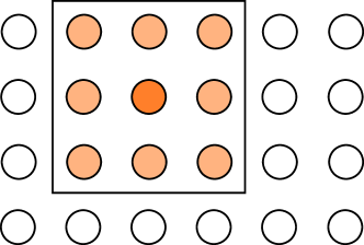
Figure 1: An illustration of hard neighbourhoods (Eq. 3) in the 2D case. This is a 4x6 grid with $K=24$ nodes. Considering the left-bottom corner node as the origin (0, 0), the eight neighbours of the node (2, 2) are highlighted.

Relation to Hebbian Learning.

We note that the online algorithm of Eqs. 1-2 can be also interpreted (see also Yin (2008) on this relation) as a variant of Hebbian learning (Hebb, 1949). Using the dot product based similarity function for $\delta$ in Eq. 1, and by defining $\mathrm{hardmax}:\mathbb{R}^{K}\rightarrow\mathbb{R}^{K}$ as the function that outputs 1 for the largest entry of the input vector, and 0 for all others, we can express Eqs. 1-2 in a fully matrix-form by defining a one-hot vector ${\bm{y}}_{t}\in\mathbb{R}^{K}$,

$${\bm{y}}_{t} =\mathrm{hardmax}({\bm{W}}_{t-1}{\bm{x}}_{t})$$ (6)

$${\bm{W}}_{t} ={\bm{W}}_{t-1}+(\beta{\bm{A}}^{(t-1)}{\bm{y}}_{t})\otimes({\bm{x}}_{t}-{\bm{W}}_{t-1}^{\intercal}{\bm{y}}_{t})$$ (7)

where $\otimes$ denotes outer product. With the neighbourhood reduced to zero, this is essentially the winner-take-all Hebbian learning. While this relation is not central to this work, we come back to this when we discuss the differentiable version of KSOM later in Sec. 5.

In passing, we also note that the last term in Eqs. 2 and 7 corresponds to Oja (1982)’s forgetting term which is not part of the original 1982 algorithm (Kohonen, 1982) but has been added later (see, e.g., Kohonen (2001)).

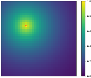
(a) Early training

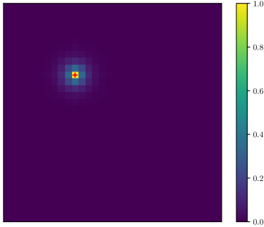
(b) Mid training

Figure 2: An illustration of Gaussian neighbourhoods in the 2D case with shrinking (Eq. 5) at two different stages of training.

2.2 Batch Algorithm & Relation to K-means

The algorithm described above is an online algorithm which updates weights after every input. The batch version thereof (Kohonen (1999, 2001); see also Cottrell et al. (2018)), which takes into account all data points $({\bm{x}}_{1},...,{\bm{x}}_{T})$ for a single update of $\{{\bm{w}}_{1},...,{\bm{w}}_{K}\}$, can be defined as follows.

At each iteration step $t$, we compute the best matching unit for each input $x_{i}$ for all $i\in\{1,..,T\}$ (we now use the sub-script $i$ to index data points not to confuse it with the iteration index $t$). Each input $x_{i}$ is a member of one of the $K$ clusters. The results can be summarised for each cluster $k\in\{1,..,K\}$ as the set $\mathcal{C}_{k}^{(t)}$ containing indices of its members at step $t$. We denote its cardinality by $|\mathcal{C}_{k}^{(t)}|$. The batch algorithm updates the weight vector ${\bm{w}}_{k}^{(t)}$ for cluster $k$ as the average of its members and their neighbours weighted by the neighbourhood coefficients. That is, ${\bm{w}}_{k}^{(t)}$ is computed as the quotient of the sum ${\bm{m}}_{k}^{(t)}$ of all inputs belonging to the corresponding cluster $k$ and their neighbours weighted by the neighbourhood coefficients, and the corresponding weighted count $N_{k}^{(t)}$, i.e.,

$${\bm{m}}_{k}^{(t)} =\sum_{j=1}^{K}{\bm{A}}_{j,k}^{(t-1)}\sum_{i\in\mathcal{C}_{j}^{(t)}}{\bm{x}}_{i}$$ (8)

$$N_{k}^{(t)} =\sum_{j=1}^{K}{\bm{A}}_{j,k}^{(t-1)}|\mathcal{C}_{j}^{(t)}|$$ (9)

$${\bm{w}}_{k}^{(t)} ={\bm{m}}_{k}^{(t)}/N_{k}^{(t)}$$ (10)

Remark 2.1 (Relation to K-means).

In the case where the neighbourhood is reduced to zero, i.e., for all $t$, ${\bm{A}}_{i,i}^{(t)}=1$ and for all $i,j$ such that $i\neq j$, ${\bm{A}}_{i,j}^{(t)}=0$, Eqs. 8-10 reduce to the standard K-means algorithm (Lloyd, 1982). Similarly, in such a case, Eqs. 1-2 reduce to an online K-means algorithm (MacQueen, 1967).

For deep learning applications, the algorithm needs to be both online and mini-batch; we discuss the corresponding extensions in Sec. 3.

2.3 Topographical Maps in the Brain as Motivation

The sub-sections above describe how KSOM performs clustering, i.e., vector quantisation. Here we discuss another property of this algorithm which is topological mapping.

It is known that there are multiple levels of topographical maps in the brain. For example, different regions of the brain specialise to different types of sensory inputs (vision, audio, touch, etc), and e.g., within the somatosensory part, regions that are responsible for different parts of the body are ordered according to the anatomical order in the body. A famous illustration of this is the “sensory homunculus.”

The design of KSOM is inspired by such topographical maps. Many have proposed computational mechanisms to achieve such a property in the 1970s/80s (von der Malsburg, 1973; von der Malsburg & Willshaw, 1977; Willshaw & von der Malsburg, 1979, 1976; Amari, 1980). Kohonen (1982) achieves this by introducing the concept of neighbourhoods between the (output) neurons. In the algorithm above (Sec. 2.1), all output neurons first compete against each other (Eq. 1) to yield a winner neuron. Then, the update is distributed to neurons that are spatially close to the winner through the coefficients of the neighbourhood matrix (Eqs. 2 and 8). As a result, clusters whose indices are spatially close on the grid are encouraged to store inputs that are close to each other in the feature space.

This is an unconventional feature for artificial NNs, since unlike the biological ones, artificial NNs do not have any physical constraints; there is no geometry nor distance between neurons. KSOM’s neighbourhoods introduce such a structure. From the machine learning perspective, the resulting topological ordering has limited practical benefits. Even if it may potentially facilitate interpretation via direct visualisation, other embedding visualisation tools could fit the bill equally well. From the neuroscience perspective, however, it may be a property that contributes in filling the gap between artificial NNs and the biological ones (see also Constantinescu et al. (2016)).

3 Alternative VQ in VQ-VAEs

The general idea of this work is to replace the VQ algorithm used in standard VQ-VAEs by Kohonen’s algorithm (Sec. 2). While the method can be applied to various data modalities, we focus on image processing as a representative example.

3.1 Background: VQ-VAEs

Let $d_{\text{in}},d_{\text{emb}},N,K$ be positive integers. A VQ-VAE (van den Oord et al., 2017) consists of an encoder NN, $\mathtt{Enc}:\mathbb{R}^{d_{\text{in}}}\rightarrow\mathbb{R}^{N\times d_{\text{emb}}}$, a decoder NN, $\mathtt{Dec}:\mathbb{R}^{N\times d_{\text{emb}}}\rightarrow\mathbb{R}^{d_{\text{in}}}$, and a codebook of size $K$ whose weights are $({\bm{w}}_{1},...,{\bm{w}}_{K})$ with ${\bm{w}}_{k}\in\mathbb{R}^{d_{\text{emb}}}$ for $k\in\{1,...,K\}$. The encoder transforms an input ${\bm{x}}\in\mathbb{R}^{d_{\text{in}}}$ to a sequence of $N$ embedding vectors $({\bm{e}}_{1},...,{\bm{e}}_{N})={\bm{E}}$ with ${\bm{e}}_{i}\in\mathbb{R}^{d_{\text{emb}}}$ for $i\in\{1,...,N\}$. Each of these embeddings is quantised to yield $(\mathtt{VQ}({\bm{e}}_{1}),...,\mathtt{VQ}({\bm{e}}_{N}))={\bm{E}}^{\prime}$ with $\mathtt{VQ}({\bm{e}}_{i})\in\mathbb{R}^{d_{\text{emb}}}$ for $i\in\{1,...,N\}$ where $\mathtt{VQ}$ denotes the VQ operation. The decoder transforms the quantised embeddings ${\bm{E}}^{\prime}$ to a reconstruction of the original input $\hat{{\bm{x}}}\in\mathbb{R}^{d_{\text{in}}}$. The corresponding operations can be expressed as follows.

$$({\bm{e}}_{1},...,{\bm{e}}_{N}) =\mathtt{Enc}({\bm{x}})$$ (11)

$$\text{For all}\,\,i\in\{1,...,N\},\,\,k_{i}^{*} =\underset{1\leq k\leq K}{\operatorname*{arg\,min}}\,\|{\bm{e}}_{i}-{\bm{w}}_{k}\|_{2}$$ (12)

$${\bm{E}}^{\prime}=(\mathtt{VQ}({\bm{e}}_{1}),...,\mathtt{VQ}({\bm{e}}_{N})) =({\bm{w}}_{k_{1}^{*}},...,{\bm{w}}_{k_{N}^{*}})$$ (13)

$$\hat{{\bm{x}}} =\mathtt{Dec}({\bm{E}}^{\prime})$$ (14)

The parameters of the encoder and decoder are trained to minimise the following loss:

$$\|{\bm{x}}-\hat{{\bm{x}}}\|_{2}^{2}+\alpha\dfrac{1}{N}\sum_{i=1}^{N}\|\mathtt{sg}({\bm{w}}_{k_{i}^{*}})-{\bm{e}}_{i}\|_{2}^{2}$$ (15)

where the first term is the reconstruction loss, and the second term is the so-called commitment loss, weighted by a hyper-parameter $\alpha\in\mathbb{R}_{>0}$, which encourages the encoder to output embeddings that are close to their quantised counterparts ($\mathtt{sg}$ denotes “stop gradient” operation to prevent gradients to propagate through ${\bm{w}}_{k_{i}^{*}}$). As noted in van den Oord et al. (2017), by assuming a uniform prior over the discrete latents, the standard KL term of the VAE loss (Kingma & Welling, 2014) can be omitted as a constant. In the reconstruction term, as the quantisation operation is non-differentiable, the straight-through estimator (Hinton, 2012; Bengio et al., 2013) is used, i.e., gradients are directly copied from the decoder input to the encoder output.

The weights of the codebook prototypes $({\bm{w}}_{1},...,{\bm{w}}_{K})$ are trained by a variant of online mini-batch K-means algorithm which keeps track of exponential moving averages (EMAs) of two quantities for each cluster $k$: the sum of updates ${\bm{m}}_{k}^{(t)}$, and the count of members in the cluster $N_{k}^{(t)}$. Their quotient yields the estimate of the weights at step $t$. Using the same notation $\mathcal{C}_{k}^{(t)}$ as in Sec. 2.2 for the set of encoder output indices (ranging from 1 to $N*B$ where $B$ is a positive integer denoting the batch size) that are members of cluster $k$ at step $t$, and by denoting encoder outputs in the batch as $({\bm{e}}_{1},...,{\bm{e}}_{N*B})$, it yields:

$${\bm{m}}_{k}^{(t)} =(1-\beta){\bm{m}}_{k}^{(t-1)}+\beta\sum_{i\in\mathcal{C}_{k}^{(t)}}{\bm{e}}_{i}^{(t)}$$ (16)

$$N_{k}^{(t)} =(1-\beta)N_{k}^{(t)}+\beta|\mathcal{C}_{k}^{(t)}|$$ (17)

$${\bm{w}}_{k}^{(t)} ={\bm{m}}_{k}^{(t)}/N_{k}^{(t)}$$ (18)

where $\alpha=1-\beta$ is the EMA decay typically set to $0.99$ (i.e., $\beta=0.01$). For shorthand, we refer to this algorithm as EMA-VQ.

While it is also possible to train these codebook parameters through gradient descent by introducing an extra term in the loss of Eq. 15 (batching is omitted for consistency): $1/N\sum_{i=1}^{N}\|{\bm{w}}_{k_{i}^{*}}-\mathtt{sg}({\bm{e}}_{i})\|_{2}^{2}$, van den Oord et al. (2017) recommend the EMA-based approach above, and many later works (Razavi et al., 2019; Ozair et al., 2021) follow this practice, while in VQ-GANs (Esser et al., 2021; Yu et al., 2022a), the gradient-based approach is also commonly used.

3.2 Kohonen-VAEs

We use KSOM (Sec. 2) as the VQ algorithm to learn the codebook weights in VQ-VAEs (Sec. 3.1). Essentially, we replace the EMA-VQ algorithm of Eqs. 16-18 by an online mini-batch version of KSOM. Such an algorithm can be obtained by introducing exponential moving averaging into the batch version of KSOM (Eqs. 8-10) with a decay of $1-\beta$. That is, we keep track of EMAs of both the weighted sum of the updates (${\bm{m}}_{k}^{(t)}$; Eq. 8) and the weighted count of members ($N_{k}^{(t)}$; Eq. 9) for each cluster $k\in\{1,...,K\}$ (where weights are the neighbourhood coefficients). Their quotient yields the estimate of the weights of codebook prototypes at step $t$. Using the same notations as in Sec. 3.1, i.e., $\mathcal{C}_{k}^{(t)}$ denotes the set of indices of encoder outputs that are members of cluster $k$ at step $t$, and $({\bm{e}}_{1},...,{\bm{e}}_{N*B})$ denotes the encoder outputs in the batch, it yields:

$${\bm{m}}_{k}^{(t)} =(1-\beta){\bm{m}}_{k}^{(t-1)}+\beta\sum_{j=1}^{K}{\bm{A}}_{j,k}^{(t-1)}\sum_{i\in\mathcal{C}_{j}^{(t)}}{\bm{e}}_{i}^{(t)}$$ (19)

$$N_{k}^{(t)} =(1-\beta)N_{k}^{(t)}+\beta\sum_{j=1}^{K}{\bm{A}}_{j,k}^{(t-1)}|\mathcal{C}_{j}^{(t)}|$$ (20)

$${\bm{w}}_{k}^{(t)} ={\bm{m}}_{k}^{(t)}/N_{k}^{(t)}$$ (21)

All other aspects are kept the same as in the basic VQ-VAE (Sec. 3.1). We refer to this approach as Kohonen-VAE.

Remark 3.1 (Relation to EMA-VQ).

If the neighbourhood is reduced to zero (see, Remark 2.1), this approach falls back to the standard EMA-VQ VAEs (Sec. 3.1).

3.3 Initialisation & Updates of EMAs

Initialisation.

Both the basic EMA-VQ (Sec. 3.1) and KSOM (Sec. 3.2) require to initialise two EMAs: ${\bm{m}}_{k}^{(0)}$ (Eq. 16 and 19) and $N_{k}^{(0)}$ (Eq. 17 and 20). This is an important detail which is omitted in the common description of VQ-VAEs. Standard public implementations of VQ-VAEs, including the official one by van den Oord et al. (2017), initialise ${\bm{m}}_{k}^{(0)}$ by a random Gaussian vector, and $N_{k}^{(0)}$ by $0$. The latter is problematic for the following reason.

In fact, standard implementations apply the updates of Eqs. 16-18 to all clusters including those that have no members in the batch—later, we show that this is another important detail for EMA-VQ. Since $N_{k}^{(0)}$ is initialised with $0$, $N_{k}^{(1)}$ remains $0$ at the first iteration for the clusters with no members in the first batch. To avoid division by zero, smoothing over counts $(N_{1}^{(t)},...,N_{K}^{(t)})$—typically additive smoothing; see, e.g., Chen & Goodman (1999)—is applied to obtain smoothed counts $(\tilde{N}_{1}^{(t)},...,\tilde{N}_{K}^{(t)})$ such that $N_{k}^{(1)}=0$ becomes $\tilde{N}_{k}^{(1)}=\epsilon$ where typically $\epsilon\sim 10^{-5}$. While this allows to avoid division by zero, the resulting multiplication of ${\bm{m}}_{k}^{(1)}$ by $1/\epsilon\sim 10^{5}$ in Eq. 18 also seems unreasonable. Our experiments (Sec. 4.1) show that this effectively results in certain sub-optimality in training. Instead, we propose $N_{k}^{(0)}=1$ initialisation, which is consistent with non-zero initialisation of ${\bm{m}}_{k}^{(0)}$.

Updating EMAs of Clusters without Members.

Given the update equations above (Eqs. 16-18 and 19-21), there remains the question whether the EMAs of clusters that have no members in the batch should be updated. As mentioned already in the previous paragraph, standard implementations update all EMAs. We conduct the corresponding ablation study in Sec. 4.1, and empirically show that, indeed, it is crucial to update all EMAs in the baseline EMA-VQ algorithm used in VQ-VAEs to achieve optimal performance.

In the next section, we’ll also show that, unlike the standard EMA-VQ which is sensitive to these configurations, KSOM is robust, and performs well under any configurations.

4 Experiments

The goal of our experiments is to revisit the properties of KSOM when integrated into VQ-VAEs. In particular, we demonstrate its robustness, and analyse learned representations. Before that, we start with showing the sensitivity of the standard EMA-VQ w.r.t. various configuration details.

4.1 Sensitivity of the baseline EMA-VQ

We first present two sets of experiments for the baseline EMA-VQ, which reveal its sensitivity to initialisation and update schemes of EMAs, as discussed in Sec. 3.3.

Improving Initialisation. We start with evaluating $N_{k}^{(0)}=1$ initialisation (instead of the standard $N_{k}^{(0)}=0$) discussed in Sec. 3.3. Figure 3 shows the evolution of the validation reconstruction loss of VQ-VAEs trained with EMA-VQ on CIFAR-10 (Krizhevsky, 2009) for two runs of 10 seeds each with $N_{k}^{(0)}=0$ (denoted by N=0/run1 and N=0/run2), and one run of 10 seeds with $N_{k}^{(0)}=1$ (denoted by N=1). In both runs with N=0, we observe a plateau at the beginning of training. The variability of the results is also high: the performance of one of them (N=0/run1; the blue curve) remains above that of the N=1 case, even after the plateau, while the other one (N=0/run2, the orange curve) successfully reaches the performance of N=1. The final/best validation reconstruction losses ($\times 10^{3}$) achieved by the respective configurations are: $148.7\pm 299.7$ vs. $52.1\pm 0.6$. In contrast, such a variability was not observed with $N_{k}^{(0)}=1$.

Updating Clusters without Members.

Now we also evaluate the effect of updating EMAs for the clusters that have no members in the batch. Table 1 shows the corresponding results. In all cases (with or without $N_{k}^{(0)}=1$ initialisation), updating all clusters including those that have no member is crucial for good performance of the baseline EMA-VQ.

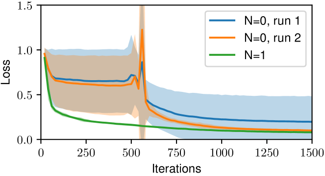
Figure 3: Evolution of validation reconstruction loss on CIFAR-10 for baseline EMA-VQ with different initialisations $N_{k}^{(0)}$ in Eq. 9.

4.2 Reconstruction Performance and Speed

We evaluate the reconstruction performance and convergence speed of VQ-VAEs trained with KSOM. We conduct experiments on three datasets: CIFAR-10 (Krizhevsky, 2009), ImageNet (Deng et al., 2009), and a mixture of CelebA-HQ (Karras et al., 2018) and Animal Faces HQ (AFHQ; Choi et al. (2020)). We use the basic VQ-VAE architecture (van den Oord et al., 2017) for CIFAR-10 and its extension VQ-VAE-2 (Razavi et al., 2019) for ImageNet and CelebA-HQ/AFHQ without architectural modifications. Further experimental details can be found in Appendix A.

Comparison to Optimised EMA-VQ.

We first compare models trained with KSOM with those trained using carefully configured EMA-VQ (Sec. 4.1). Table 2 summarises the results. We first observe that all methods achieve a similar validation reconstruction loss, with slight improvements obtained by KSOM over the baseline on CelebA-HQ/AFHQ. To compare the “speed of convergence,” we measure the number of steps needed by each algorithm to achieve $+10\%$ and $+20\%$ of their final performance. Here “steps” correspond to the number of updates, and the batch size is the same for all methods. We observe that, indeed, KSOM tends to be faster than the basic EMA-VQ at the beginning of training, as can be seen in the column $+20\%$ (especially for the hard variant on CelebA-HQ/AFHQ). However, the baseline catches up later, and the difference becomes rather marginal at the $+10\%$ threshold: the corresponding speed up by KSOM is less than 5% relative compared to carefully configured EMA-VQ. In what follows, we show that KSOM is much more robust than EMA-VQ, and performs well under all configurations, including those that are sub-optimal for EMA-VQ.

Table 1: Sensitivity of the baseline EMA-VQ. VQ-VAEs trained with EMA-VQ on CIFAR-10. “$N_{k}^{(0)}$” indicates its initialisation with 0 or 1. “Update-0” indicates whether to update clusters that have 0 members in the batch. “# Steps” is the number of training steps needed to achieve +10% of the final loss. Mean and std are computed using 10 seeds. For the $N_{k}^{(0)}=0$ case, there is a high variability among results even with 10 seeds, as we report in Sec. 4.1: here, we report the result obtained using 10 good seeds.

$N_{k}^{(0)}$	Update-0	Loss ($\times 10^{3}$)	# Steps ($\times 10^{3}$)
0	No	148.8 $\pm$ 11.0	13.5 $\pm$ 0.7
1	No	68.3 $\pm$   0.8	16.3 $\pm$ 1.4
0	Yes	52.1 $\pm$ 0.6	6.8 $\pm$ 0.6
1	Yes	51.9 $\pm$ 0.2	5.4 $\pm$ 0.5

Table 2: Validation reconstruction loss and number of steps needed to achieve +10% and +20% of the final loss for various Kohonen-VAEs. “None” in column “Neighbours” corresponds to our well-configured EMA-VQ (Sec. 4.1; “$N_{k}^{(0)}=1$” and “Update-0, Yes” in Table 3). 2D grid is used for both “Hard” and “Gaussian” cases. Mean and standard deviations are computed with 10 seeds for CIFAR-10 and 5 seeds each for ImageNet and CelebA-HQ/AFHQ. Image resolution is 32x32 for CIFAR-10 and 256x256 for ImageNet and CelebA-HQ/AFHQ.

	CIFAR-10			ImageNet			CelebA-HQ/AFHQ
		# Steps ($\times 10^{3}$)			# Steps ($\times 10^{3}$)			# Steps ($\times 10^{3}$)
Neighbours	Loss ($\times 10^{3}$)	+10%	+20%	Loss ($\times 10^{3}$)	+10%	+20%	Loss ($\times 10^{4}$)	+10%	+20%
None	51.9 $\pm$ 0.2	5.4 $\pm$ 0.5	3.7 $\pm$ 0.5	23.0 $\pm$ 0.4	15.2 $\pm$ 1.6	8.4 $\pm$ 0.6	18.6 $\pm$ 1.0	17.0 $\pm$ 1.0	14.1 $\pm$ 1.4
Hard	52.1 $\pm$ 0.2	5.2 $\pm$ 0.6	2.5 $\pm$ 0.5	23.5 $\pm$ 0.4	13.6 $\pm$ 2.2	7.4 $\pm$ 0.9	17.3 $\pm$ 0.1	17.0 $\pm$ 1.6	10.8 $\pm$ 1.3
Gaussian	51.8 $\pm$ 0.2	5.2 $\pm$ 0.6	3.0 $\pm$ 0.0	23.2 $\pm$ 0.4	14.0 $\pm$ 1.4	7.6 $\pm$ 0.6	17.5 $\pm$ 0.3	17.8 $\pm$ 1.8	11.8 $\pm$ 1.3

Table 3: Validation reconstruction loss and number of steps needed to achieve +10% of the final loss (“# Steps”), showing the robustness of KSOM w.r.t. configurations that are sub-optimal for EMA-VQ. “$N_{k}^{(0)}$” indicates its initialisation with 0 or 1. “Update-0” indicates whether to update clusters that have 0 members in the batch. Numbers for the hard variant are reported (results are similar for Gaussian).

			CIFAR-10		ImageNet		CelebA-HQ/AFHQ
	$N_{k}^{(0)}$	Update-0	Loss ($\times 10^{3}$)	# Steps ($\times 10^{3}$)	Loss ($\times 10^{3}$)	# Steps ($\times 10^{3}$)	Loss ($\times 10^{4}$)	# Steps ($\times 10^{3}$)
EMA-VQ	0	No	148.8 $\pm$ 11.0	13.5 $\pm$ 0.7	44.7 $\pm$ 2.6	13.5 $\pm$ 0.7	$37.3\pm 1.2$	$21.2\pm 3.9$
KSOM			51.8 $\pm$   0.2	5.2 $\pm$ 0.6	24.4 $\pm$ 1.3	12.6 $\pm$ 0.9	17.4 $\pm$ 0.4	17.6 $\pm$ 3.6
EMA-VQ	1	No	68.3 $\pm$ 0.8	16.3 $\pm$ 1.4	27.9 $\pm$ 1.0	21.2 $\pm$ 1.5	$30.1\pm 2.8$	$22.6\pm 0.5$
KSOM			52.1 $\pm$ 0.3	4.8 $\pm$ 0.9	24.1 $\pm$ 1.3	12.2 $\pm$ 1.3	17.4 $\pm$ 0.2	16.6 $\pm$ 1.5
EMA-VQ	0	Yes	52.1 $\pm$ 0.6	6.8 $\pm$ 0.6	23.6 $\pm$ 0.9	15.4 $\pm$ 2.7	$18.0\pm 1.0$	$17.6\pm 1.5$
KSOM			51.9 $\pm$ 0.2	4.8 $\pm$ 0.6	23.7 $\pm$ 0.7	14.2 $\pm$ 1.6	17.2 $\pm$ 0.1	16.8 $\pm$ 1.9

Robustness of KSOM against EMA-VQ Issues.

Above we report that the performance gain (both in speed and reconstruction quality) by KSOM is rather marginal compared to our carefully configured EMA-VQ baseline obtained in Sec. 4.1. Here we compare the two approaches under various configurations. Table 3 shows the results. We observe that KSOM is remarkably robust: in all configurations, including those that are sub-optimal for EMA-VQ, KSOM achieves the same best validation loss as in the optimal configuration (Table 2). KSOM’s neighbourhood updating scheme naturally fixes the problematic cases of the original EMA-VQ above. In these configurations, KSOM also generally converges faster than the baseline EMA-VQ. These results hold for both VQ-VAEs trained on CIFAR-10 and for VQ-VAE-2s trained on ImageNet and CelebA-HQ/AFHQ. In addition, in Appendix B.1, we show that KSOM also tends to improve the codebook utilisation.

4.3 Topologically Ordered Discrete Representations

Finally, we analyse the discrete representations learned by KSOM. We show that they are “topologically” ordered on the grid of indices, and consequently, reconstructed images remain close to the original ones even when we slightly shift their latent representations in the discrete index space.

Grid Visualisation.

We first visualise how learned discrete representations are distributed over the grid. Here we use a VQ-VAE trained with KSOM (2D with hard neighbourhoods) on CIFAR-10, and proceed as follows. A discrete latent representation consists of $N$ integers (Sec. 3.1). For each index in the codebook (corresponding to one of the nodes on the grid), we create a discrete latent representation whose $N$ codes are all the same and equal to the corresponding index, and feed it to the decoder to obtain an output image. This results in a grid of images shown in Figure 4. We observe that each code seems to correspond to some colour, we can effectively observe several local “islands” of colours which group colours that are visually close.

Impact of Perturbation in the Discrete Latent Space.

To further illustrate the presence of neighbourhoods developed by KSOM in the discrete latent space, we show images obtained by perturbing the discrete latent code representing a proper image in the index space (by adding or subtracting an integer offset to each coordinates of the code indices). Here we use VQ-VAE-2 trained on ImageNet with 2D KSOM with hard neighbourhoods. The VQ-VAE-2 (Razavi et al., 2019) has two levels of discretisation: we shift all of them by the same offset on both $x$ and $y$ axes of the 2D grid for KSOM or directly shift the code indices for EMA-VQ. Figure 5 shows the results. Obviously, with the baseline VQ-VAE-2 trained with EMA-VQ, the output images become complete noises under such perturbations, even with an offset of one. With the KSOM-trained representations, there is a certain degree of continuity in the space of indices (as illustrated in Figure 4): the output images preserve the original contents though they become noisier as the offset increases. This illustrates the neighbourhoods learned by KSOM.

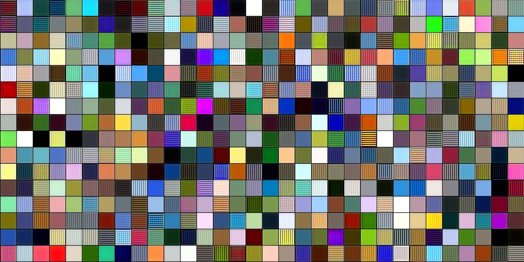
(a) EMA-VQ

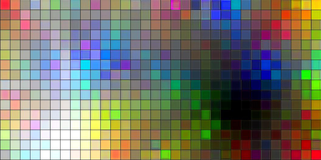
(b) KSOM

Figure 4: A visualization of codebook ($K=512$) of VQ-VAEs trained on CIFAR10 with (a) EMA-VQ or (b) KSOM. The codebook of EMA-VQ obviously has no structure but serves as a reference. Similar visualisations for VQ-VAE-2 trained on ImageNet can be found in Appendix B.3.

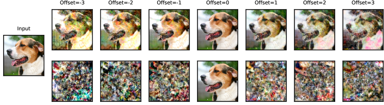
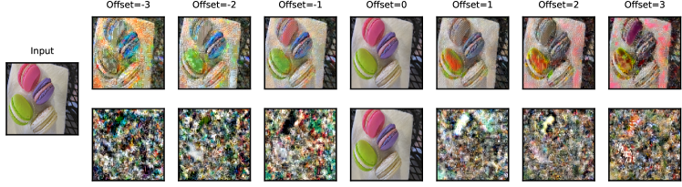
Figure 5: Effects of perturbations to the discrete latent code on reconstructed images. For each image, the top row shows the results for KSOM, and the bottom row shows those for EMA-VQ. “Offset” indicates the offset added to the indices of the latent representations.

5 Discussion

Recommendations.

Our first recommendation for any EMA-VQ implementation is to modify $N_{k}^{(0)}=0$ to $N_{k}^{(0)}=1$ (Sec. 4.1). For a more robust solution, we recommend using KSOM. Extending the standard implementation of EMA-VQ (Sec. 3.1) to KSOM (Sec. 3.2) is straightforward. While we introduce one extra hyper-parameter, shrink step $\tau$ (Eqs. 4-5), we found $\tau=0.1$ to perform well across all tasks. Regarding the model variations, we recommend using the 2D variant with hard neighbourhoods. Virtually, any VQ implementation should benefit from these modifications.

Related Work.

The work that is the most related to ours is Fortuin et al. (2019)’s SOM-VAE which is also inspired by KSOM. The core difference between the SOM-VAE and our approach is that Fortuin et al. (2019) train the codebook weights by gradient descent: The gradients of the codebook weights are copied to the neighbour weights. While this is indeed inspired by Kohonen’s neighbourhoods, none of Kohonen’s learning rules (Sec. 2) is used. Also, the main focus of Fortuin et al. (2019) is on modelling and interpreting time series. In fact, SOM-VAEs are extended by Manduchi et al. (2021) for further applications to heath care.

There are also several other works which attempt to improve the VQ algorithm. For example, Zeghidour et al. (2021) propose to initialise all codebook weights using examples in the first batch. Lee et al. (2022) propose residual VQ that iteratively performs VQ for improved reconstruction quality.

Applications of VQ.

Following the VQ-VAE of van den Oord et al. (2017), VQ has become popular across various modalities and applications. Besides the standard use case for high-dimensional data such as images, audio, and video, VQ has been also used for texts. For example, Kaiser et al. (2018); Roy et al. (2018) downsample target sentences via VQ to speed up decoding in machine translation. Liu & Niehues (2022) explore VQ to improve multi-lingual translation. Ozair et al. (2021) applies VQ to model-based reinforcement learning/planning by quantising state-action sequences. Many text-to-image generation systems also include VQ components, e.g., Ramesh et al. (2021) make use of discrete VAEs with Gumbel-softmax (Jang et al., 2017)), and Yu et al. (2022b) build upon VQ-GAN-2 (Yu et al., 2022a). Discrete representation learning is also motivated by out-of-distribution (or systematic) generalisation in certain tasks (Liu et al., 2021, 2022; Träuble et al., 2022).

Differentiable Relaxation of KSOM.

While working very well in practice, the use of the straight-through estimator (Sec. 3.1) to pass the gradients through the quantisation operation seems sub-optimal at first. For example, Agustsson et al. (2017) show the possibility to perform discrete representation learning in fully differentiable NNs by using softmax with temperature annealing. In fact, we can also naturally derive a differentiable version of KSOM by replacing $\mathrm{hardmax}$ in Eq. 6 (presented in Sec. 2) by the softmax function. However, in our preliminary experiments, none of our differentiable variants with temperature annealing obtained a successful model that achieves a good reconstruction loss when the softmax is discretised for testing.

Semantic Codebook.

While we demonstrate the emergence of neighbourhoods in the discrete space of codebook indices learned by KSOM, the features encoded by them remain low-level (mostly colours). While learning of more “semantic” discrete codes is out of scope here, we expect KSOM with such representations to be even more interesting, as it may potentially enable interpolation in the discrete latent space.

6 Conclusion

We revisit the learning rule of Kohonen’s Self-Organising Maps (KSOM) as the vector quantisation (VQ) algorithm for discrete representation learning in NNs. KSOM is a generalisation of the exponential moving-average based VQ algorithm (EMA-VQ) commonly used in VQ-VAEs. We empirically demonstrate that, unlike the standard EMA-VQ, KSOM is robust w.r.t. initialisation and EMA update schemes. Our recipes can easily be integrated into existing code for VQ-VAEs. In addition, we show that discrete representations learned by KSOM effectively develop topological structures. We provide illustrations of the learned neighbourhoods in the image domain.

Appendix A Experimental Details

Datasets.

We use three datasets (one of them is a mixture of two standard datasets): CIFAR-10 (Krizhevsky, 2009), ImageNet (Deng et al., 2009), and a mixture of CelebA-HQ (Karras et al., 2018) and Animal Faces HQ (AFHQ; Choi et al. (2020)). The number of images and the resolution we use are: 60 K and 32x32, 1.3 M and 256x256, 43 K (the sum of 28 K for CelebA-HQ and 15 K for AFHQ) and 256x256, respectively. For any further details, we refer the readers to the original references.

Model Architectures.

We use the basic configuration (including hyper-parameters) of VQ-VAE (van den Oord et al., 2017) for CIFAR-10 and that of VQ-VAE-2 (Razavi et al., 2019) for ImageNet and CelebA-HQ/AFHQ from the original papers. The only change we introduce is the learning algorithm to train the codebook weights (Sec. 3.2). Again, for any further details on the model architectures, we refer the readers to the original references above. The dimension of latent representation for VQ-VAE on CIFAR-10 is 8x8x64, i.e, $N=8\times 8=64$ and $d_{\text{emb}}=64$ using our notations of Sec. 3.1. VQ-VAE-2 has two codebooks (“top” and “bottom”) with respective embedding dimensions of 32x32x64 ($N=32\times 32$) and 64x64x64 ($N=64\times 64$) with $d_{\text{emb}}=64$ for both. We use the codebook size of $K=512$ everywhere for all datasets.

Reference Baseline Implementations.

We looked into several public implementations of the baseline VQ-VAEs, including the original implementation of VQ-VAE/EMA-VQ https://github.com/deepmind/sonnet/blob/v2/sonnet/src/nets/vqvae.py, its PyTorch re-implementation https://github.com/zalandoresearch/pytorch-vq-vae (see also https://github.com/lucidrains/vector-quantize-pytorch), and VQ-VAE-2 https://github.com/rosinality/vq-vae-2-pytorch. The GitHub link to our code can be found on the first page.

Appendix B Extra Experimental Results

Here we provide several extra experimental results which we could not report in the main text due to space limitation.

B.1 Codebook Utilisation

Here we show that KSOM also helps boosting the codebook utilisation of VQ-VAE and VQ-VAE-2. As a measure of codebook utilisation, we compute perplexity for each batch as $\exp(\sum_{k=1}^{K}p(k)\log(p(k)))$ where $p(k)=C(k)/(N*B)$ with $C(k)$ denoting the number of times the code $k$ is used in the batch (with a batch size $B$ and the number of embeddings $N$; the same notation as in the main text). Figure 6 shows the evolution of perplexity on all datasets (for VQ-VAE-2s, we show that for the two codebooks). With the only exception of the “bottom” codebook of VQ-VAE-2 trained on CelebA-HQ/AFHQ, overall, we observe that the code utilisation of KSOM variants tends to be higher than that of the baseline EMA-VQ. In particular, for the “top” codebook of VQ-VAE-2 trained on CelebA-HQ/AFHQ (Figure 6 (d)), the hard KSOM’s mean perplexity exceeds 300 while the baseline EMA-VQ’s is below 100.

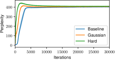
(a) CIFAR-10, VQ-VAE

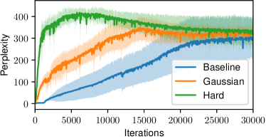
(b) ImageNet, VQ-VAE-2, Top

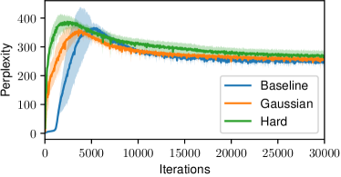
(c) ImageNet, VQ-VAE-2, Bottom

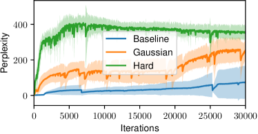
(d) CelebA-HQ/AFHQ, VQ-VAE-2, Top

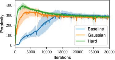
(e) CelebA-HQ/AFHQ, VQ-VAE-2, Bottom

Figure 6: Evolution of perplexity (codebook utilisation) as a function of training iterations. The codebook size is $K=512$ in all cases. “Baseline” is the standard EMA-VQ. “Hard” and “Gaussian” indicate the corresponding neighbourhood type for KSOM.

B.2 Ablation Studies

In the main text, we show that the performances of the hard and Gaussian variants are rather close (Table 2). We also conduct ablation studies to compare 1D vs. 2D grids, and different values of shrinking step $\tau\in\{1,0.1,0.01\}$, and observe that these different variations yield rather similar performance. For the sake of completeness, Table 4 presents the corresponding results. In terms of neighbourhoods, as expected, we find that the variants with small shrinking steps $\tau$ of $0.01$ or $0.1$ yield smoother codebook grids than those obtained with $\tau=1$.

Table 4: Ablation studies on the 1d/2D grid and shrinking step size $\tau$. Validation reconstruction loss and number of steps needed to achieve +10% and +20% of the final loss. Mean and standard deviations are computed with 10 seeds for CIFAR-10 and 5 seeds each for CelebA-HQ/AFHQ. Image resolution is 32x32 for CIFAR-10 and 256x256 for CelebA-HQ/AFHQ. The best numbers for “hard” and “Gaussian” groups are highlighted in bold separately.

		CIFAR-10			CelebA-HQ/AFHQ
			# Steps ($\times 10^{3}$)			# Steps ($\times 10^{3}$)
Neighbours	$\tau$	Loss ($\times 10^{3}$)	+10%	+20%	Loss ($\times 10^{4}$)	+10%	+20%
Hard 1D	0.1	52.0 $\pm$ 0.2	$5.3\pm 0.5$	$3.1\pm 0.3$	$17.4\pm 0.2$	15.8 $\pm$ 0.8	10.8 $\pm$ 1.5
Hard 2D	1	$52.1\pm 0.4$	4.7 $\pm$ 0.7	2.6 $\pm$ 0.5	$17.4\pm 0.2$	$18.0\pm 1.6$	$11.4\pm 1.1$
Hard 2D	0.1	52.0 $\pm$ 0.3	4.9 $\pm$ 0.3	2.4 $\pm$ 0.5	17.3 $\pm$ 0.2	$18.0\pm 1.6$	$12.4\pm 1.1$
Hard 2D	0.01	$52.1\pm 0.3$	$5.5\pm 0.7$	$3.0\pm 0.0$	$17.6\pm 0.3$	$17.0\pm 2.9$	$12.4\pm 2.1$
Gaussian 1D	0.1	$51.9\pm 0.4$	$5.2\pm 0.4$	$3.1\pm 0.3$	$17.8\pm 0.5$	$18.0\pm 2.7$	11.6 $\pm$ 1.3
Gaussian 2D	1	$51.9\pm 0.2$	$5.3\pm 0.5$	$3.3\pm 0.5$	$18.3\pm 0.4$	16.4 $\pm$ 1.9	11.8 $\pm$ 1.8
Gaussian 2D	0.1	$51.8\pm 0.3$	5.1 $\pm$ 0.3	3.1 $\pm$ 0.3	$17.6\pm 0.2$	$18.6\pm 2.1$	$13.2\pm 0.8$
Gaussian 2D	0.01	51.7 $\pm$ 0.2	$5.4\pm 0.5$	$3.6\pm 0.5$	17.5 $\pm$ 0.5	$18.4\pm 2.6$	$11.8\pm 1.3$

B.3 More Visualisations for VQ-VAE-2

Grid Visualisation for VQ-VAE-2.

In Figure 4 in the main text, we visualise the 2D grid representation of the codebook for a VQ-VAE trained on CIFAR-10. Here we show similar visualisations for VQ-VAE-2 trained on ImageNet. One complication for such visualisations for VQ-VAE-2 is that it has two codebooks (“top” and “bottom”). We therefore cannot exhaustively visualise all combinations. We show a few of them by fixing all codes in either the top or bottom representations, and varying the others. Figure 7 shows the results. While hue/value/saturation change for different values of fixed top or bottom code, we again observe many “islands” of similar colours grouped together.

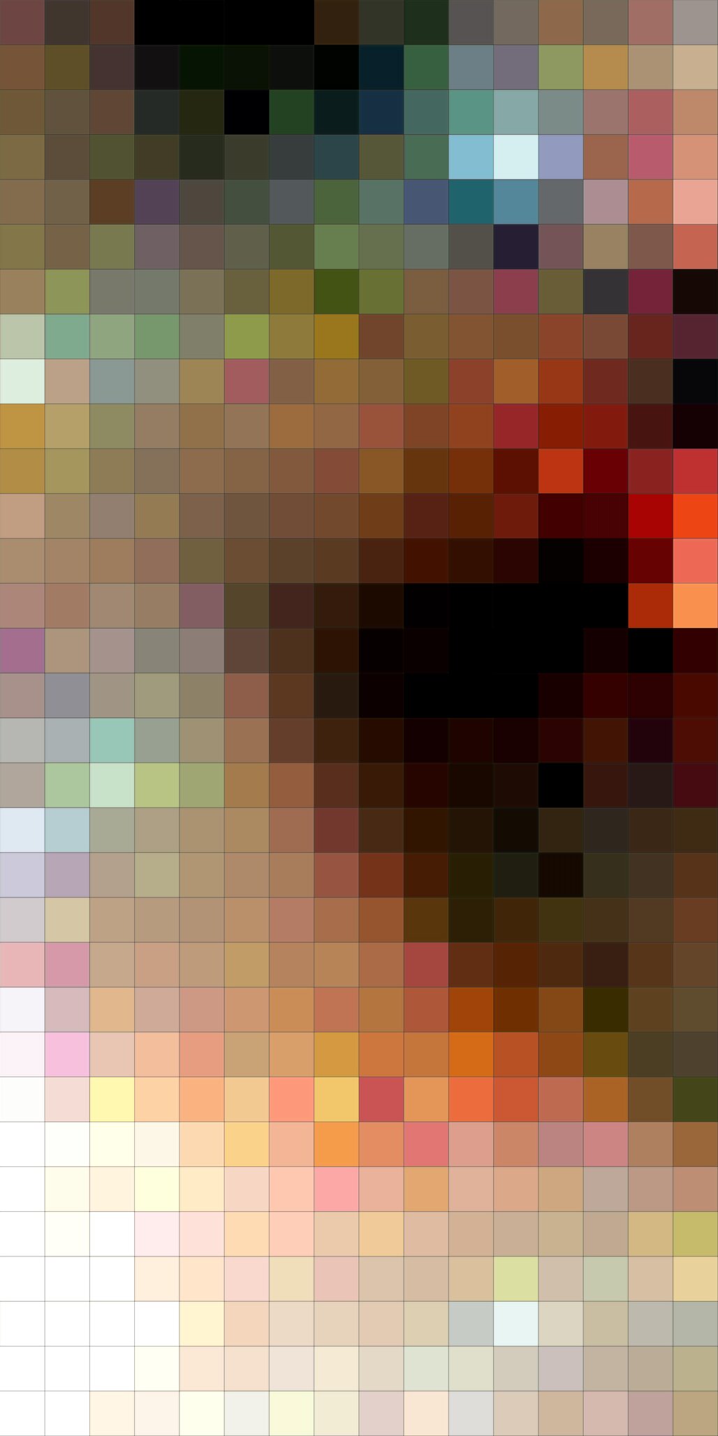
(a) Top=(0, 0)

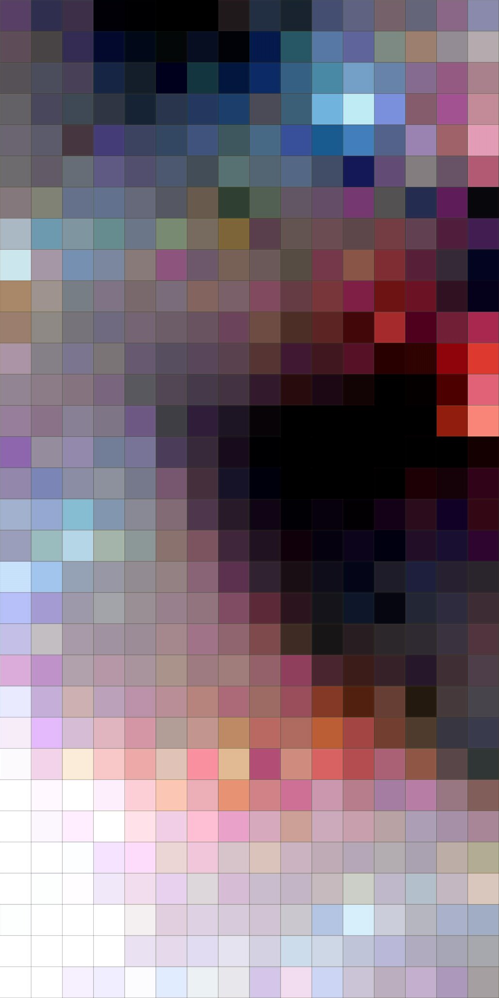
(b) Top=(18, 15)

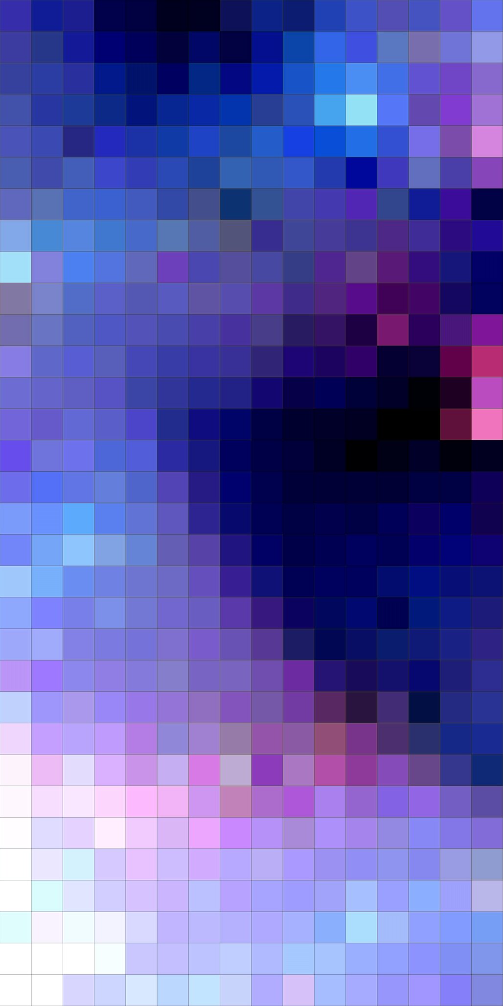
(c) Top=(27, 3)

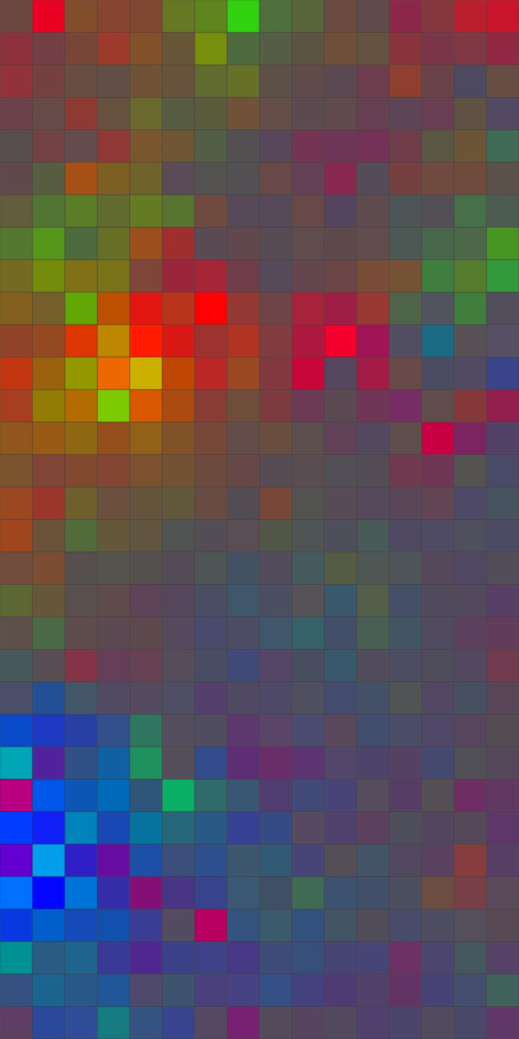
(d) Bottom=(0, 0)

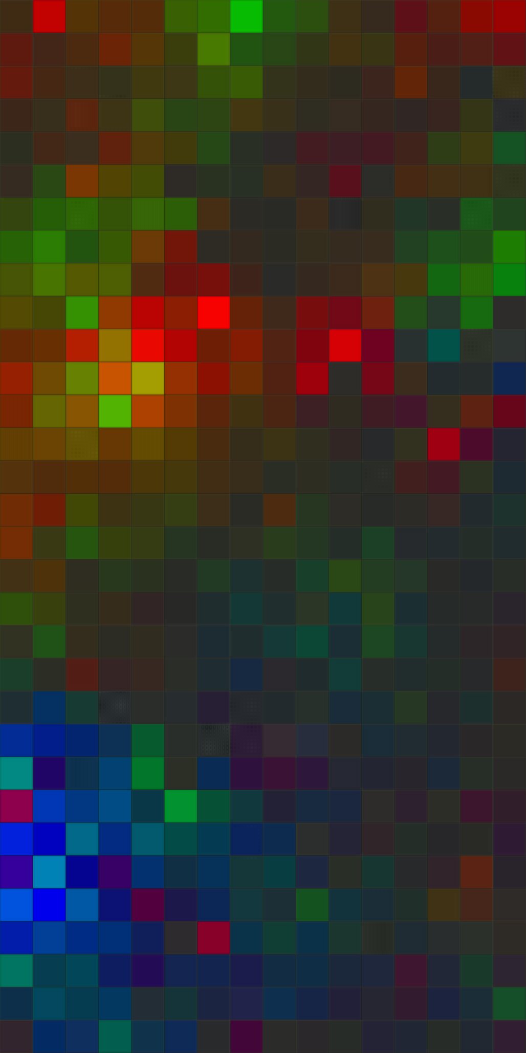
(e) Bottom=(18, 15)

(f) Bottom=(27, 3)

Figure 7: Codebook visualisations for VQ-VAE-2 trained on ImageNet with 2D-Hard KSOM. The description in the caption specifies which of the top or bottom latent representations is fixed to which coordinates.

Perturbing only one of the two latent representations in VQ-VAE-2.

In Figure 5 in the main text, we apply an offset to all indices in the two latent representations (“top” and “bottom”) of VQ-VAE-2. Here we show the effect of perturbing only one of the two latent representations, i.e., we keep one of the “top” or “bottom” latent representations fixed (to that of a proper image), and apply offsets to the other one. Figures 8 and 9 show the corresponding results. Since one of the two latent representations is fixed, the “contents” of the original image is somewhat preserved in all cases. The comparison is interesting in the case where we perturb the top latent code: in the KSOM case, the changes of top latent code seem to gradually affect the hue/value of the image.

(a) KSOM, shift top representation

(b) KSOM, shift bottom representation

(c) EMA-VQ Baseline, shift top representation

(d) EMA-VQ Baseline, shift bottom representation

Figure 8: Effects of perturbing only one of the top or bottom latent representations in VQ-VAE-2 (“dog”)

(a) KSOM, shift top representation

(b) KSOM, shift bottom representation

(c) EMA-VQ Baseline, shift top representation

(d) EMA-VQ Baseline, shift bottom representation

Figure 9: Effects of perturbing only one of the top or bottom latent representations in VQ-VAE-2 (“macaron”)

References

- Agustsson et al. (2017) Agustsson, E., Mentzer, F., Tschannen, M., Cavigelli, L., Timofte, R., Benini, L., and Gool, L. V. Soft-to-hard vector quantization for end-to-end learning compressible representations. In Proc. Advances in Neural Information Processing Systems (NIPS), pp. 1141–1151, December 2017.
- Amari (1980) Amari, S.-I. Topographic organization of nerve fields. Bulletin of Mathematical Biology, 42(3):339–364, 1980.
- Baevski et al. (2020) Baevski, A., Schneider, S., and Auli, M. vq-wav2vec: Self-supervised learning of discrete speech representations. In Int. Conf. on Learning Representations (ICLR), Virtual only, April 2020.
- Bengio et al. (2013) Bengio, Y., Léonard, N., and Courville, A. Estimating or propagating gradients through stochastic neurons for conditional computation. Preprint arXiv:1308.3432, 2013.
- Borsos et al. (2022) Borsos, Z., Marinier, R., Vincent, D., Kharitonov, E., Pietquin, O., Sharifi, M., Teboul, O., Grangier, D., Tagliasacchi, M., and Zeghidour, N. AudioLM: a language modeling approach to audio generation. Preprint arXiv:2209.03143, 2022.
- Chen & Goodman (1999) Chen, S. F. and Goodman, J. An empirical study of smoothing techniques for language modeling. Computer Speech & Language, 13(4):359–393, 1999.
- Choi et al. (2020) Choi, Y., Uh, Y., Yoo, J., and Ha, J. StarGAN v2: Diverse image synthesis for multiple domains. In Proc. IEEE Conf. on Computer Vision and Pattern Recognition (CVPR), pp. 8185–8194, Virtual only, June 2020.
- Constantinescu et al. (2016) Constantinescu, A. O., O’Reilly, J. X., and Behrens, T. E. Organizing conceptual knowledge in humans with a gridlike code. Science, 352(6292):1464–1468, 2016.
- Cottrell et al. (2018) Cottrell, M., Olteanu, M., Rossi, F., and Villa-Vialaneix, N. Self-organizing maps, theory and applications. Revista de Investigacion Operacional, 39(1):1–22, 2018.
- Csordás et al. (2022) Csordás, R., Irie, K., and Schmidhuber, J. CTL++: Evaluating generalization on never-seen compositional patterns of known functions, and compatibility of neural representations. In Proc. Conf. on Empirical Methods in Natural Language Processing (EMNLP), Abu Dhabi, UAE, December 2022.
- De Bodt et al. (2004) De Bodt, E., Cottrell, M., Letremy, P., and Verleysen, M. On the use of self-organizing maps to accelerate vector quantization. Neurocomputing, 56:187–203, 2004.
- Deng et al. (2009) Deng, J., Dong, W., Socher, R., Li, L., Li, K., and Fei-Fei, L. ImageNet: A large-scale hierarchical image database. In Proc. IEEE Conf. on Computer Vision and Pattern Recognition (CVPR), pp. 248–255, Miami, Florida, USA, June 2009.
- Dhariwal et al. (2020) Dhariwal, P., Jun, H., Payne, C., Kim, J. W., Radford, A., and Sutskever, I. Jukebox: A generative model for music. Preprint arXiv:2005.00341, 2020.
- Esser et al. (2021) Esser, P., Rombach, R., and Ommer, B. Taming transformers for high-resolution image synthesis. In Proc. IEEE Conf. on Computer Vision and Pattern Recognition (CVPR), pp. 12873–12883, Virtual only, June 2021.
- Fortuin et al. (2019) Fortuin, V., Hüser, M., Locatello, F., Strathmann, H., and Rätsch, G. SOM-VAE: interpretable discrete representation learning on time series. In Int. Conf. on Learning Representations (ICLR), New Orleans, LA, USA, May 2019.
- Hebb (1949) Hebb, D. O. The organization of behavior; a neuropsycholocigal theory. A Wiley Book in Clinical Psychology, 62:78, 1949.
- Hinton (2012) Hinton, G. Neural networks for machine learning. Coursera, video lectures, 2012.
- Hupkes et al. (2019) Hupkes, D., Singh, A., Korrel, K., Kruszewski, G., and Bruni, E. Learning compositionally through attentive guidance. In Proc. Int. Conf. on Computational Linguistics and Intelligent Text Processing, La Rochelle, France, April 2019.
- Jang et al. (2017) Jang, E., Gu, S., and Poole, B. Categorical reparameterization with gumbel-softmax. In Int. Conf. on Learning Representations (ICLR), Toulon, France, April 2017.
- Kaiser et al. (2018) Kaiser, L., Bengio, S., Roy, A., Vaswani, A., Parmar, N., Uszkoreit, J., and Shazeer, N. Fast decoding in sequence models using discrete latent variables. In Proc. Int. Conf. on Machine Learning (ICML), pp. 2395–2404, Stockholm, Sweden, July 2018.
- Karras et al. (2018) Karras, T., Aila, T., Laine, S., and Lehtinen, J. Progressive growing of GANs for improved quality, stability, and variation. In Int. Conf. on Learning Representations (ICLR), Vancouver, Canada, April 2018.
- Kingma & Welling (2014) Kingma, D. P. and Welling, M. Auto-encoding variational bayes. In Int. Conf. on Learning Representations (ICLR), Banff, Canada, April 2014.
- Kohonen (1982) Kohonen, T. Self-organized formation of topologically correct feature maps. Biological cybernetics, 43(1):59–69, 1982.
- Kohonen (1999) Kohonen, T. Comparison of SOM point densities based on different criteria. Neural Computation, 11(8):2081–2095, 1999.
- Kohonen (2001) Kohonen, T. Self-organizing maps. Springer (the first edition published in 1995), 2001.
- Krizhevsky (2009) Krizhevsky, A. Learning multiple layers of features from tiny images. Master’s thesis, Computer Science Department, University of Toronto, 2009.
- Lee et al. (2022) Lee, D., Kim, C., Kim, S., Cho, M., and Han, W.-S. Autoregressive image generation using residual quantization. In Proc. IEEE Conf. on Computer Vision and Pattern Recognition (CVPR), pp. 11523–11532, New Orleans, LA, USA, June 2022.
- Liska et al. (2018) Liska, A., Kruszewski, G., and Baroni, M. Memorize or generalize? searching for a compositional RNN in a haystack. In AEGAP Workshop ICML, Stockholm, Sweden, July 2018.
- Liu & Niehues (2022) Liu, D. and Niehues, J. Learning an artificial language for knowledge-sharing in multilingual translation. In Proc. Conf. on Machine Translation (WMT), pp. 188–202, Abu Dhabi, December 2022.
- Liu et al. (2021) Liu, D., Lamb, A., Kawaguchi, K., Goyal, A., Sun, C., Mozer, M. C., and Bengio, Y. Discrete-valued neural communication. In Proc. Advances in Neural Information Processing Systems (NeurIPS), pp. 2109–2121, Virtual only, December 2021.
- Liu et al. (2022) Liu, D., Lamb, A., Ji, X., Notsawo, P., Mozer, M., Bengio, Y., and Kawaguchi, K. Adaptive discrete communication bottlenecks with dynamic vector quantization. Preprint arXiv:2202.01334, 2022.
- Lloyd (1982) Lloyd, S. Least squares quantization in PCM. IEEE Transactions on Information Theory, 28(2):129–137, 1982.
- MacQueen (1967) MacQueen, J. Classification and analysis of multivariate observations. In Proc. Berkeley Symp. Math. Statist. Probability, pp. 281–297, 1967.
- Manduchi et al. (2021) Manduchi, L., Hüser, M., Faltys, M., Vogt, J. E., Rätsch, G., and Fortuin, V. T-DPSOM: an interpretable clustering method for unsupervised learning of patient health states. In Proc. Conf. on Health, Inference, and Learning (CHIL), pp. 236–245, Virtual only, April 2021.
- Nasrabadi & Feng (1988) Nasrabadi, N. M. and Feng, Y. Vector quantization of images based upon the Kohonen self-organizing feature maps. In Proc. IEEE Int. Conf. on Neural Networks (ICNN), volume 1, pp. 101–105, 1988.
- Oja (1982) Oja, E. Simplified neuron model as a principal component analyzer. Journal of mathematical biology, 15(3):267–273, 1982.
- Ozair et al. (2021) Ozair, S., Li, Y., Razavi, A., Antonoglou, I., van den Oord, A., and Vinyals, O. Vector quantized models for planning. In Proc. Int. Conf. on Machine Learning (ICML), pp. 8302–8313, Virtual only, July 2021.
- Ramesh et al. (2021) Ramesh, A., Pavlov, M., Goh, G., Gray, S., Voss, C., Radford, A., Chen, M., and Sutskever, I. Zero-shot text-to-image generation. In Proc. Int. Conf. on Machine Learning (ICML), volume 139, pp. 8821–8831, Virtual only, December 2021.
- Razavi et al. (2019) Razavi, A., van den Oord, A., and Vinyals, O. Generating diverse high-fidelity images with VQ-VAE-2. In Proc. Advances in Neural Information Processing Systems (NeurIPS), pp. 14837–14847, Vancouver, Canada, December 2019.
- Rombach et al. (2022) Rombach, R., Blattmann, A., Lorenz, D., Esser, P., and Ommer, B. High-resolution image synthesis with latent diffusion models. In Proc. IEEE Conf. on Computer Vision and Pattern Recognition (CVPR), pp. 10674–10685, New Orleans, LA, USA, June 2022.
- Roy et al. (2018) Roy, A., Vaswani, A., Parmar, N., and Neelakantan, A. Towards a better understanding of vector quantized autoencoders. OpenReview, 2018.
- Schlag et al. (2021) Schlag, I., Irie, K., and Schmidhuber, J. Linear Transformers are secretly fast weight programmers. In Proc. Int. Conf. on Machine Learning (ICML), Virtual only, July 2021.
- Schmidhuber (1991) Schmidhuber, J. Learning to control fast-weight memories: An alternative to recurrent nets. Technical Report FKI-147-91, Institut für Informatik, Technische Universität München, March 1991.
- Tirunagari et al. (2016) Tirunagari, S., Bull, S., Kouchaki, S., Cooke, D., and Poh, N. Visualisation of survey responses using self-organising maps: a case study on diabetes self-care factors. In Proc. IEEE Symposium Series on Computational Intelligence (SSCI), pp. 1–6, 2016.
- Tjandra et al. (2020) Tjandra, A., Sakti, S., and Nakamura, S. Transformer VQ-VAE for unsupervised unit discovery and speech synthesis: Zerospeech 2020 challenge. In Proc. Interspeech, pp. 4851–4855, Virtual only, October 2020.
- Träuble et al. (2022) Träuble, F., Goyal, A., Rahaman, N., Mozer, M., Kawaguchi, K., Bengio, Y., and Schölkopf, B. Discrete key-value bottleneck. Preprint arXiv:2207.11240, 2022.
- van den Oord et al. (2017) van den Oord, A., Vinyals, O., and Kavukcuoglu, K. Neural discrete representation learning. In Proc. Advances in Neural Information Processing Systems (NIPS), pp. 6306–6315, Long Beach, CA, December 2017.
- Vaswani et al. (2017) Vaswani, A., Shazeer, N., Parmar, N., Uszkoreit, J., Jones, L., Gomez, A. N., Kaiser, Ł., and Polosukhin, I. Attention is all you need. In Proc. Advances in Neural Information Processing Systems (NIPS), pp. 5998–6008, Long Beach, CA, USA, December 2017.
- von der Malsburg (1973) von der Malsburg, C. Self-organization of orientation sensitive cells in the striate cortex. Kybernetik, 14(2):85–100, 1973.
- von der Malsburg & Willshaw (1977) von der Malsburg, C. and Willshaw, D. J. How to label nerve cells so that they can interconnect in an ordered fashion. Proc. the National Academy of Sciences, 74(11):5176–5178, 1977.
- Walker et al. (2021) Walker, J., Razavi, A., and Oord, A. v. d. Predicting video with VQVAE. Preprint arXiv:2103.01950, 2021.
- Willshaw & von der Malsburg (1976) Willshaw, D. J. and von der Malsburg, C. How patterned neural connections can be set up by self-organization. Proceedings of the Royal Society of London. Series B. Biological Sciences, 194(1117):431–445, 1976.
- Willshaw & von der Malsburg (1979) Willshaw, D. J. and von der Malsburg, C. A marker induction mechanism for the establishment of ordered neural mappings: its application to the retinotectal problem. Philosophical Transactions of the Royal Society of London. B, Biological Sciences, 287(1021):203–243, 1979.
- Yan et al. (2021) Yan, W., Zhang, Y., Abbeel, P., and Srinivas, A. VideoGPT: Video generation using vq-vae and transformers. Preprint arXiv:2104.10157, 2021.
- Yin (2008) Yin, H. The self-organizing maps: background, theories, extensions and applications. In Computational intelligence: A compendium, pp. 715–762. 2008.
- Yu et al. (2022a) Yu, J., Li, X., Koh, J. Y., Zhang, H., Pang, R., Qin, J., Ku, A., Xu, Y., Baldridge, J., and Wu, Y. Vector-quantized image modeling with improved VQGAN. In Int. Conf. on Learning Representations (ICLR), Virtual only, April 2022a.
- Yu et al. (2022b) Yu, J., Xu, Y., Koh, J. Y., Luong, T., Baid, G., Wang, Z., Vasudevan, V., Ku, A., Yang, Y., Ayan, B. K., et al. Scaling autoregressive models for content-rich text-to-image generation. Preprint arXiv:2206.10789, 2022b.
- Zeghidour et al. (2021) Zeghidour, N., Luebs, A., Omran, A., Skoglund, J., and Tagliasacchi, M. Soundstream: An end-to-end neural audio codec. IEEE/ACM Transactions on Audio, Speech, and Language Processing, 30:495–507, 2021.