Online Tool Selection with Learned Grasp Prediction Models Technical Report

Date: © OSARO Inc. All rights reserved. Materials may not be published, broadcast, rewritten, or redistributed without express written consent of OSARO Inc.

Abstract

Deep learning-based grasp prediction models have become an industry standard for robotic bin-picking systems. To maximize pick success, production environments are often equipped with several end-effector tools that can be swapped on-the-fly, based on the target object. Tool-change, however, takes time. Choosing the order of grasps to perform, and corresponding tool-change actions, can improve system throughput; this is the topic of our work. The main challenge in planning tool change is uncertainty – we typically cannot see objects in the bin that are currently occluded. Inspired by queuing and admission control problems, we model the problem as a Markov Decision Process (MDP), where the goal is to maximize expected throughput, and we pursue an approximate solution based on model predictive control, where at each time step we plan based only on the currently visible objects. Special to our method is the idea of void zones, which are geometrical boundaries in which an unknown object will be present, and therefore cannot be accounted for during planning. Our planning problem can be solved using integer linear programming (ILP). However, we find that an approximate solution based on sparse tree search yields near optimal performance at a fraction of the time. Another question that we explore is how to measure the performance of tool-change planning: we find that throughput alone can fail to capture delicate and smooth behavior, and propose a principled alternative. Finally, we demonstrate our algorithms on both synthetic and real world bin picking tasks.

1 Introduction

Automated bin picking has gained considerable attention from manufacturing, e-commerce order fulfillment, and warehouse automation. The problem generally involves grasping of a diverse set of novel objects, which are often packed randomly inside a bin (Figure 1(b)). A common model-free bin picking approach is based on learning grasp prediction models – deep neural networks that map an image of the bin to success probabilities for different grasps [ZSY⁺18, LLS15] (see Figures 1(c) and 1(d) for examples of learned grasp prediction models for two different vacuum suctions with diameters $30$mm and $50$mm respectively).

In order to handle a diverse range of objects, robotic cells are often equipped with a tool changer mechanism (Figure 1(a)), allowing the robot to select a new end-effector from a set of available end-effectors (e.g., vacuum end-effectors varying in size, antipodal end-effectors) and swap it with the current one automatically in real time (for example $50$mm vacuum end-effector grasp prediction model depicted in Figure 1(d) places more probability mass over the larger objects, while $30$mm vacuum end-effector grasp prediction model model depicted in Figure 1(d) places more probability mass over the smaller objects for the example bin image given in Figure 1(b)). Choosing the right tool for each object can increase the pick success, potentially leading to improved throughput. Tool changing, however, comes at a cost of cycle time: navigating the end-effector to the tool changing station, and performing the swap.

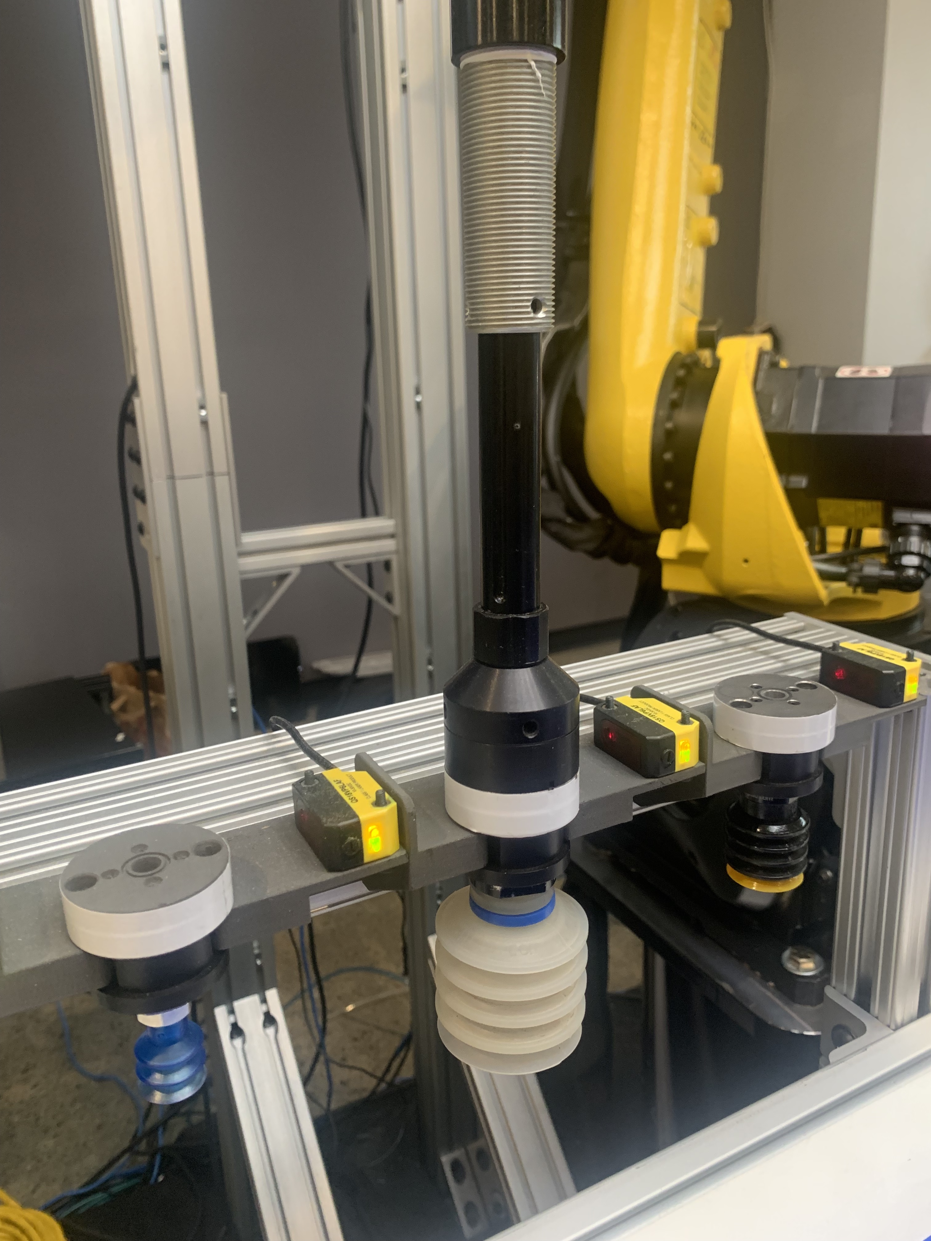
(a)

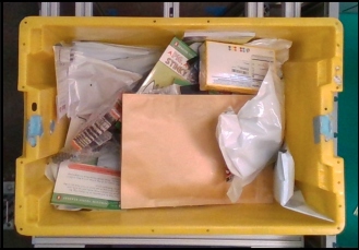
(b)

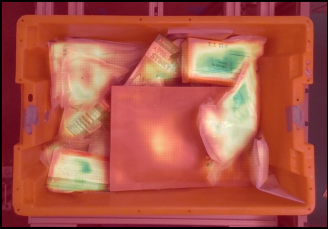
(c)

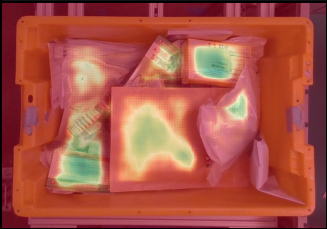
(d)

Figure 1: (a) Tool-changer station hosting different vacuum end-effectors of various sizes. The current selection is already mounted on the robot; (b) Example of a bin containing an assortment of various objects; (c) and (d) depict grasp score heat maps for a $30$mm and a $50$mm vacuum suction cups respectively (green spectrum denotes higher grasp scores). Note that the grasp prediction model for vacuum suction cup $50$mm generally places more probability mass over the larger objects compared to the $30$mm vacuum suction cup.

In common picking tasks, the agent is free to choose the order of objects to pick, and respectively, the order of tool changes. Thus, by carefully planning the picking order, we can potentially improve picking efficiency, by, e.g., using the same tool repeatedly for several objects. This is our main objective in this work. Optimizing tool selection, however, is challenging due to several reasons. Typically, some objects in the bin are occluded, and even objects that are currently visible may move unexpectedly due to grasp attempts of nearby objects, affecting their optimal tool selection in the future. Furthermore, even if the objects positions were known in advance, the complexity of computing the optimal picking order scales exponentially with the planning horizon, and is effectively intractable for real-time operation. Our goal in this work is to develop a scalable, well-performing, and fast method for approximately optimal tool selection.

We present a general formulation of this stochastic decision making problem, which we term Grasp Tool Selection Problem (GTSP), as a Markov Decision Process (MDP) (Section 2). In practice, solving this MDP is difficult due to its large state space and difficult-to-estimate transition dynamics. To address this, we introduce an approximation of the problem where we: (1) replace the discounted horizon problem with a receding horizon Model Predictive Control (MPC); (2) In the inner planning loop of the MPC component, we replace the stochastic optimization with an approximate deterministic problem that does not require the complete knowledge of the true transition dynamics. We show that this deterministic problem is an instance of integer linear programming (ILP), which can be solved using off-the-shelf software packages. However, we further show that an approximate solution method based on a sparse tree search improves the planning speed by orders of magnitude, with a negligible effect on the solution quality, and is fast enough to run in real time.

Our approach decouples grasp prediction learning from tool selection planning – we only require access to a set of pre-trained grasp prediction models for each individual end-effector. Thus, our method can be applied ad hoc in production environments whenever such models are available. In our experiments, on both synthetic and real-world environments, we demonstrate that our planning method significantly improves system throughput when compared to heuristic selection methods. Another novel contribution of this work is the derivation of a set of metrics for benchmarking tool selection algorithms, based on practical considerations relevant to the bin picking problem.

Related Work

There is extensive literature on learning grasp prediction models [LPKQ16, RA15, MMS⁺19]. To the best of our knowledge, few previous studies considered tool change optimization. The closest related work is [MMS⁺19] in the context of controlling an ambidextrous robot for bin picking problem. That work focused on scaling the learning of the grasp prediction models, and not on the tool selection problem. In their approach, the best tool is selected greedily based on the grasp prediction scores generated by the end-effector grasp prediction models. Tackling problems with uncertain transitions by replanning using deterministic models is a common approach in planning [RN95] and robotics, where it is commonly referred to as model predictive control [CA13, TTZ⁺16]. To our knowledge, this work is the first application of this idea to tool change optimization with learned grasp models. Several studies focused on planning with deep visual predictors [FL16, EFLL17, EFD⁺18, XELF19], where a deep visual predictive model is learned and combined with MPC. Our work differs from these approaches in that we perform planning directly in grasp proposal space, based on our void zone approximation.

2 Grasp Tool Selection Problem (GTSP) Formulation

We assume a planar workspace $\mathcal{I}$, discretized into a grid of $W\times H$ points. For example, $\mathcal{I}$ could be the bin image, as in Figure 1(b), where every pixel maps to a potential grasp point in the robot frame. A grasp proposal evaluates the probability of succeeding in grasping at a particular point. Formally, a grasp proposal is a tuple $\omega\coloneqq\{\mathcal{E},u,\rho\}$, where $\mathcal{E}$ is an end-effector, $u\in\mathcal{I}$ is a position to perform a grasp (e.g., a pixel in the image), and $0\leq\rho\leq 1$ is the probability of a successful grasp when the end-effector $\mathcal{E}$ is used to perform a grasp on position $u$. We also use the notations $\omega^{\mathcal{E}},\omega^{u}$, and $\omega^{\rho}$ when referring to individual elements of a grasp proposal $\omega$.

A grasp prediction model $\Gamma_{\mathcal{E}}:\mathcal{I}\rightarrow\{\omega_{i}\}_{i=1}^{W\times H}$ gives a set of grasp proposals for an input image $\mathcal{I}$ and end-effector $\mathcal{E}$. In practice, only a small subset of grasp proposals yield good grasps. Thus, without loss of generality, we denote $\Gamma^{k}_{\mathcal{E}}(\mathcal{I})=\{\omega_{i}\}_{i=1}^{k}$, limiting the model only to the $k$ best grasps (in terms of grasp success probability). Given a set of $n$ end-effector grasp proposal models $\{\Gamma_{i}\}_{i=1}^{n}$, we define the grasp plan space $\Omega\coloneqq\cup_{i=1}^{n}\Gamma^{k}_{i}(\mathcal{I})$, which denotes the space of all plannable grasps. We will further denote by $\Omega_{t}$ the grasp plan space that is available at time $t$ of the task.

Grasp Tool Selection Problem (GTSP):

We model the problem as a Markov Decision Process (MDP [Ber12]) $\mathcal{M}\equiv\langle\mathcal{S},\mathcal{A},\mathcal{R},\mathcal{T}\rangle$ defined as follows: $\mathcal{S}$ is a set of states, where each $s=\langle\Omega,\mathcal{E}\rangle\in\mathcal{S}$ consists of the current grasp plan space and the current end-effector on the robot. We denote by $s^{\Omega}$ and $s^{\mathcal{E}}$ the individual elements of state $s$. The action space $\mathcal{A}=\Omega$ is the set of all plannable grasp proposals. The reward balances pick success and tool change cost, and we chose it as:

$${\mathcal{R}}(s,\omega)=\hskip 0.72229pt\omega^{\rho}+c\hskip 1.4457pt\mathbf{1}(s^{\mathcal{E}}\neq\omega^{\mathcal{E}}),$$ (1)

where $\omega^{\rho}$ is the grasp success score, $c<0$ reflects a negative reward for tool changing, and $\mathbf{1}(\cdot)$ is the indicator function. The state transition function $\mathcal{T}(s_{t},\omega_{t},s_{t+1})\rightarrow[0,1]$ gives the probability of observing the next state $s_{t+1}$ after executing grasp proposal $\omega_{t}$ in state $s_{t}$. As a result of performing a grasp, and depending on the grasp outcome, an object is removed from the bin and some other object randomly appears at the position of the executed grasp and new graspable positions will be exposed. The optimal policy $\pi^{*}:\mathcal{S}\to\Omega$ is defined as: $\pi^{*}=\operatorname*{argmax}_{\pi}\operatorname{\mathbb{E}}_{\pi}\left[\sum_{t=0}^{\infty}\gamma^{t}\mathcal{R}(s_{t},\omega_{t})|\omega_{t}\sim\pi(s_{t})\right]$.

3 Approximate GTSP Solution

Solving GTSP is difficult for following reasons: (1) Prediction: we do not know the true state transitions, as they capture the future grasps that will be made possible after a grasp attempt, which effectively requires a prediction of objects in the bin that are not directly visible (see, e.g., Figure 1(b)). Although several studies investigated learning visual predictive models (see [FL16, EFLL17, EFD⁺18, XELF19]), learning such models in production environments with a high variability of objects is not yet practical. (2) Optimization: even if the state transitions were known, the resulting MDP would have an intractable number of states, precluding the use of standard MDP optimization methods.

We address (1) by replacing the stochastic optimization with an approximate deterministic problem that does not require the complete knowledge of the true transitions, based on the idea of void zones. We address (2) by replacing the infinite horizon discounted horizon problem with an online solver, which at each time step chooses the grasp that is optimal for the next several time steps; we term this part the model predictive control (MPC) component. We propose two computational methods for solving the short horizon problem in the inner MPC loop, either accurately, based on integer linear programming (ILP) outlined in Section 3.2, or approximately, using a sparse tree search method (STS) outlined in Section 3.3.

Algorithm 1 outlines the generic Model Predictive Control (MPC) for solving the GTSP. At every step, the current observations (e.g., bin image $\mathcal{I}$) is fed to the set of pre-trained end-effector models to obtain the plan space $\Omega_{t}$. Next, a GTSP-void-Solver is called over the current state $s_{t}\leftarrow\langle\Omega_{t},\mathcal{E}_{t}\rangle$ which will return an optimized plan $\omega$, and finally the first step (i.e., grasp proposal) of the plan is executed. We have already described the ILP solver in the paper and will outline the Sparse Tree Search (STS) solver in the next section.

Algorithm 1 Model Predictive Control (MPC)

1:Inputs: Set of end-effector models $\{\Gamma_{i}\}_{i=1}^{n}$, maximum number of best grasp proposals per end-effector model to include $m$, receding horizon $H$, tool changing costs $c<0$, void radius $l$

2:for $t=1,2,\ldots$ do

3:     Observe the current bin image $\mathcal{I}_{t}$, and current end-effector $\mathcal{E}_{t}$

4:     Construct the current plan space: $\Omega_{t}\leftarrow\cup_{i=1}^{n}\Gamma^{m}_{i}(\mathcal{I}_{t})$

5:     $s_{t}\leftarrow\langle\Omega_{t},\mathcal{E}_{t}\rangle$

6:     $(\omega,v_{\omega})\leftarrow$ GTSP-void-Solver($s_{t},H,c,l$) $\triangleright$ ILP, or Sparse-Tree-Search (STS)

7:     Execute the grasp proposal $\omega$

8:end for

3.1 Approximate Prediction using Void Zones

We seek to replace the stochastic (and unknown) transitions in GTSP by deterministic dynamics, such that the solution of the deterministic problem will yield a reasonable approximation of the true optimal controller. Our approach is based on the idea of a void zone – not allow a grasp that is in very close proximity to any previous grasp, as movement of objects in the bin resulting from the previous grasp attempt could render a future grasp in its close vicinity impossible.

We motivate void zones with the following working hypothesis: As long as the objects are sufficiently small, when a grasp is attempted, the set of grasp proposals that are sufficiently distant from the attempted grasp position will remain valid in the next state.

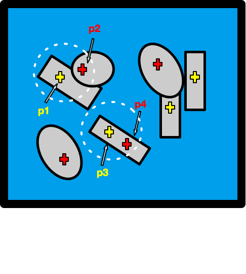
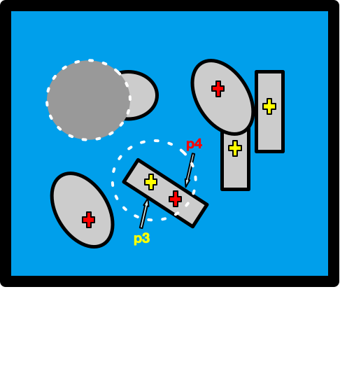
Figure 2: (Left) examples of cases where performing a grasp proposal would invalidate some other grasp proposals ($p_{1}$ invalidates $p_{2}$, and $p_{3}$ invalidates $p_{4}$); (Right) updated grasp plan space for the next horizon step by voiding the impacted grasp proposal (in this case voiding $p_{2}$ as a result of committing to the grasp proposal $p_{1}$).

This observation is illustrated in Figure 2(Left), for a bin picking problem with two end-effectors. The grasp proposals are color coded for each end-effector. In some cases, grasp proposals lie over different objects where one object might be partially occluding the other one (e.g., $p_{1}$ and $p_{2}$). In other cases, two or more grasp proposals might lie on the same object. In either case, performing one of the grasp proposals will invalidate some other grasp proposal and hence those proposals should not be available to the planner in the next steps.

We define the void zone based on the Euclidean distance, as follows:

Definition 1 (l-separation).

Let $d_{i,j}=\left\lVert\omega^{u}_{i}-\omega^{u}_{j}\right\rVert$ denote the Euclidean distance on the plane between grasp proposals $\omega_{i}$ and $\omega_{j}$. A pair of grasp proposals $\langle\omega_{i},\omega_{j}\rangle$ is called $l$-separated if $d_{i,j}>l$. We refer to $l$ as void radius and use the notation $\Psi_{l}(\omega)$ to refer to a set of grasp proposals which are l-separated from $\omega$. Note that by definition $\omega\not\in\Psi_{l}(\omega)$.

Based on the above definition, we can formally define deterministic dynamics in GTSP, which we will henceforth refer to as GTSP-void. At state $s_{t}=\langle\Omega_{t},\mathcal{E}_{t}\rangle$, taking action $\omega_{t}$ results in a next state,

$$\small s_{t+1}= \langle\Omega_{t+1},\omega^{\mathcal{E}}_{t}\rangle,$$

$$\Omega_{t+1}= \{\omega\hskip 3.61371pt|\hskip 3.61371pt\omega\in\Omega_{t}\land\omega\in\Psi_{l}(\omega_{t})\}$$ (2)

That is, the end-effector in the next state is as chosen by $\omega_{t}$, and the grasp plan space is updated to exclude all grasp proposals within the void zone.

As shown in Figure 2, by setting the void zone large enough, we can safely ignore the local changes as a result of executing a grasp. Obviously, using void zones comes at some cost of sub-optimality – as we ignore possible future grasps inside the void zones. To mitigate this cost, we propose a model predictive control (MPC) approach. At every step, the current observation (i.e., bin image $\mathcal{I}$) is fed to the set of pre-trained end-effector models to obtain the plan space $\Omega_{t}$. Next, we solve the corresponding GTSP-void problem with some fixed horizon $H$, and the first step of the plan $\omega$ is executed.

Replanning at every step allows our method to adapt to the real transitions observed in the bin. Next, we propose two methods for solving the inner GTSP-void optimiztion problem within our MPC.

3.2 Approximate Optimization using Integer Linear Programming

In this section we show that the GTSP-void problem can be formulated as an integer linear program (ILP). To motivate this approach, note that GTSP-void with horizon $H$ seeks to find a trajectory of $H$ $l$-separated grasp proposals in $\Omega_{t}$ with the highest accumulated return. This motivates us to think of the problem as a walk over a directed graph generating an elementary path of length $H$ of $l$-separated grasp proposals with the highest return, where the nodes of the graph are the grasp proposals in the current state, $s^{\Omega}_{t}$, and the directed edges represent the order at which the grasp proposals are executed. Our formulation is mainly inspired by the ILP formulation of the well known Travelling Salesman Problem (TSP) [DFJ54] with the following changes: (1) the main objective is modified to finding an elementary path of length $h$ with maximal return, anywhere on the graph (as opposed to the conventional tour definition in TSP); (2) addition of the $l$-separation constraints to enforce voiding; (3) a modification of Miller-Tucker-Zemlin sub-tour elimination technique [MTZ60] for ensuring the path does not contain any sub-tour.

Algorithm 2 Integer Linear Program (ILP)

1:Objective: $v^{*}=\underset{\omega_{ij}}{\text{max}}\sum_{w_{ij}}r_{ij}\omega_{ij}\hskip 7.22743pt\mbox{s.t.}$

2:$\omega_{ij}\in\{0,1\},\hskip 3.61371pt\forall{i,j\in\mathcal{V}}$ $\triangleright$ binary variables representing edges in the solution

3:$\sum_{j\in\mathcal{V}\backslash\{s,e\}}\omega_{sj}=1$ $\triangleright$ constraint enforcing one outgoing edge from the initial node $s$

4:$\sum_{i\in\mathcal{V}\backslash\{s,e\}}\omega_{ie}=1$ $\triangleright$ constraint enforcing one incoming edge to the terminal node $e$

5:$\sum_{i,j\in\mathcal{V}\backslash\{s,e\}}\omega_{ij}=H$ $\triangleright$ constraint enforcing the trajectory length to be exactly $H$

6:$\sum_{j\in\mathcal{V}\backslash\{s,i,e\}}\omega_{ij}=\sum_{j\in\mathcal{V}\backslash\{s,i,e\}}\omega_{ji},\hskip 3.61371pt\forall i\in\mathcal{V}\backslash\{s,e\}$

7:$\sum_{j\in\mathcal{V}\backslash\{s,i,e\}}\omega_{ij}\leq 1$ $\triangleright$ Steps $6$ and $7$ specify constraints enforcing the flow conservation

8:$\omega+\omega^{\prime}\leq 1,\hskip 3.61371pt\forall\omega\in\phi_{i},\forall\omega^{\prime}\in\phi_{j},\hskip 3.61371pt\mbox{if}\left\lVert\omega^{u}_{i}-\omega^{u}_{j}\right\rVert\leq l,\forall i,j\in\mathcal{V}\backslash\{s,e\}$ $\triangleright$ $l$-separation constraints (see text)

9:$u_{i}\in\{0,1,2,\ldots,|\mathcal{V}|\},\hskip 3.61371pt\forall{i\in\{1,\ldots,\mathcal{V}\}}$

10:$u_{1}=1$ and $u_{|\mathcal{V}|}=|\mathcal{V}|$,   $2\leq u_{i}\leq|\mathcal{V}|-1$, $\forall{i\in\{2,\ldots,|\mathcal{V}|-1\}}$

11:$u_{i}-u_{j}+1\leq(H+1)(1-\omega_{ij})$, $\forall{i,j\in\{2,\ldots,|\mathcal{V}|-1\}}$ $\triangleright$ steps $9$-$11$ specify Miller-Tucker-Zemlin (MTZ) sub-tour elimination constraints

12:return $(\omega_{i},v^{*})\hskip 3.61371pt\mbox{s.t.}\hskip 3.61371pt\omega_{si}=1$

Given the current state $s_{t}=\langle\Omega_{t},\mathcal{E}_{t}\rangle$, we represent the grasp plan space as a graph $\mathcal{G}=\langle\mathcal{V},E\rangle$ where the nodes of the graph are grasp proposals $\omega_{i}\in s^{\Omega}_{t}$ plus two auxiliary initial and terminal nodes $\{s,e\}$: $\mathcal{V}=\{1,\ldots,|\Omega_{t}|\}\cup\{s,e\}$. We index the initial and terminal nodes by $1$ and $|\mathcal{V}|$, respectively. For any pair of $l$-separated grasp proposals $\omega_{i}$ and $\omega_{j}$ ($i,j\in\mathcal{V}\backslash\{s,e\}$) we add directed edges $\{e_{ij},e_{ji}\}\in E$ with a reward $r_{ij}\coloneqq\rho_{\omega_{i}}+c\mathbf{1}{(\omega^{\mathcal{E}}_{i}\neq\omega^{\mathcal{E}}_{j})}$ (cf. Equation 1). For such pairs of grasp proposals we also add binary variables $\{\omega_{ij},\omega_{ji}\}$ to ILP. We connect the initial node $s$ to the set of all grasp proposal nodes with reward defined as $r_{si}\coloneqq c\hskip 1.4457pt\mathbf{1}{(\omega^{\mathcal{E}}_{s}\neq\omega^{\mathcal{E}}_{i}})$ and add binary variables $\omega_{si}\hskip 1.4457pt(\forall i\in\mathcal{V}\backslash\{s,e\})$ to ILP. We also connect the set of all grasp proposal nodes to the terminal node $e$ with reward $r_{ie}\coloneqq\omega^{\rho}_{i}$, and add corresponding binary variables $\omega_{ie}\hskip 1.4457pt(\forall i\in\mathcal{V}\backslash\{s,e\})$ to ILP. The optimization objective is defined as maximization $v^{*}=\underset{\omega_{ij}}{\text{max}}\sum_{w_{ij}}r_{ij}\omega_{ij}$ subject to a set of constraint that enforce an elementary path of length $H$.

The complete ILP formulation is outlined in Algorithm 2. The constraints in lines 2-7 are similar to a standard TSP formulation [DFJ54]. Constraints on line 2 enforce binary constraints on $\omega_{i,j}$ variables where $\omega_{i,j}=1$ selects the pair of grasp proposals $\omega_{i}$ and $\omega_{j}$ to be included in the solution, in that order. Constraint on line 3 ensures only one outgoing connection exists from the auxiliary start node $s$ to grasp proposal nodes (marking the start of the path). Constraint on line 4 ensures only one incoming connection exists from grasp proposal nodes to the auxiliary sink node $e$ (marking the end of the path). Constraint on line 5 enforces the length of the elementary path to be exactly $H$. Constraints on line 6 are flow conservation constraints, while the constraint on line 7 ensures that the outgoing degree of each node is at most one (standard flow conservation constraints in TSP (see [DFJ54])). Line 8 defines the $l$-separation constraints. We denote by $\phi_{i}\coloneqq\{\omega_{j,k}|j=i\vee k=i\}$ the set of all incoming and outgoing edges of the node $i$. For two nodes $i,j$ that are not $l$-separated, the constraint only allows for at most one element of $\phi_{i},\phi_{j}$ to be included in the solution. The constraints on lines 9-11 specify our adaptation of the Miller-Tucker-Zemlin sub-tour elimination technique [MTZ60]. For each node in the graph (including the source and sink nodes) we add an integer variable $u_{i}$. (with $u_{1}$ associated with the source node $s$ and $u_{|\mathcal{V}|}$ associated with the source node $e$). We enforce $u_{1}=1$ and $u_{|\mathcal{V}|}=|\mathcal{V}|$ to ensure the source node $s$ marks the start of the trajectory and the sink node $e$ marks the end of the trajectory (line 10). The rest of variables $u_{i}$ could take on values in between (line 10). These constraints, together with line 11 induces an ordering of the grasp proposals which prevents sub-tours.

3.3 Approximate Optimization using Sparse Tree Search

We now present a simple alternative to ILP for approximately solving GTSP-void  based on a sparse tree search (STS). Our approach, outlined in Algorithm 3, performs a tree search of depth $H$ where tree node expansion takes place over a sparse subset of grasp proposals respecting the l-separation constraint (see Definition 1 in Section 3.1). At every search step a node is expanded using a sparse subset of available grasp proposals (line 6). In our approach we use the union of top $k$ grasp proposals per end-effector according to the grasp proposal scores $\omega^{\rho}$. The parameter $k$ – hereafter the sparsity factor – determines the sparsity of the subset of grasp proposals for the tree search node expansion. While expanding over the set of all available grasp proposals at every node is possible and optimally solves the problem in theory, in practice it makes the planning significantly slow and hence is not suitable for real world production environments. The algorithm then recursively calculates a sub-plan rooted at that node for a receding horizon of $H$ (line 9), accumulates the results of each recursion and computes the value of the sub plan (line 10), and it returns the best sub-plan and its value among all the sub-plans calculated at that horizon.

Algorithm 3 Sparse Tree Search (STS)

1:function STS($s_{t},H,c,l,k$)$\triangleright$ current state $s_{t}=\langle\Omega_{t},\Gamma_{t}\rangle$; horizon $H$, tool changing costs $c<0$, void radius $l$, $k$ is the sparsity factor where it specifies the top $k$ grasp proposals per end-effector to be included for the search tree node expansion

2:    if $H=0$ then

3:         return $(\_,0)$

4:    end if

5:    $\Xi\leftarrow\emptyset$

6:    Let $\hskip 1.4457pt\Lambda^{k}_{t}\subset\Omega_{t}$ be the union of the top $k$ grasp proposals per end-effector (in terms of grasp score $\omega^{\rho}$) available in $\Omega_{t}$

7:    for $\omega\in\Lambda^{k}_{t}$ do $\triangleright$ $\omega=\langle\mathcal{E},u,\rho\rangle$

8:         $s_{t+1}=\mathcal{T}_{l}(s_{t},\omega)$ $\triangleright$ forward dynamics in Equation 2

9:         $(\omega^{+},v_{\omega^{+}})\leftarrow$ STS($s_{t+1},H-1,c,l,k$)

10:         $v_{\omega}=\bar{\mathcal{R}}(s_{t},\omega)+v_{\omega^{+}}$ $\triangleright$ reward function defined in Equation1

11:         $\Xi\leftarrow\Xi\cup(\omega,v_{\omega})$

12:    end for

13:    return $\operatorname*{argmax}_{v_{\omega}}(\Xi)$

14:    

15:end function

4 Experiments

We divide our presentation to an investigation on synthetic problems, aimed at quantifying our algorithmic choices, and a real robot study evaluating the performance of our method in practice.

4.1 Synthetic Experiments

In the first set of experiments we conducted a comparative analysis of the two GTSP-void solvers outlined in Sections 3.2 and 3.3. Our goal is to answer the following question: How do the ILP and STS solvers compare in terms of the optimization quality and speed?

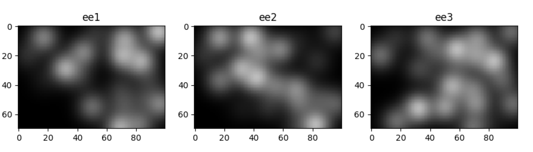
Figure 3: Synthetic end-effector grasp proposal model generation for three end-effectors generated over a fixed grid resolution $70\times 110$.

We crafted a synthetic tool selection problem generator as follows. A problem instance $\mathcal{T}$ is generated by first selecting the number of end-effectors and then, for each end-effector, we generate a random set of grasp proposals over a fixed grid resolution H$\times$W (we used H=$70$, W=$110$ in our experiments) To generate realistic grasp proposals, we first choose $n=25$ random object positions, uniformly sampled on the grid.

Next, for each-end effector we generate random Gaussian kernels with randomized scale and standard deviation, centered on each object position. The resulting grasp proposal grid for each pixel gives a higher probability of success to pixels that are closer to an object center.

Algorithm 4 outlines the pseudocode for generating synthetic experiments. Function GenerateGraspModel generates a ransom grasp proposal model for a given resolution $\langle H,W\rangle$ with higher grasp scores centered on a set of pixel positions $p^{i}=\langle p^{i}_{x},p^{i}_{y}\rangle$ (mimicking object centers).This is simply done by defining randomly scaled normal distributions with means centered on positions $p^{i}$ and random standard deviations $\sigma_{i}$. Function RunExperiment describes the main loop for generating synthetic experiments. Given an ablation over experiment parameters (i.e., number of end-effectors $n_{ee}$, horizon $h$, sparsity factor $k$, void radius $l$, tool changing costs $c<0$) and a number of episodes $N$ (for calculating the statistics), we first sample $m$ positions (mimicking object centers) and then generate $n_{ee}$ random grasp models using GenerateGraspModel. Next, we run both ILP and STS solvers and collect performance results in terms of plan value and plan time for each solver. Figure 3 shows examples of synthetic grasp map generated by this function for three end-effectors.

Algorithm 4 Synthetic Experiments

1:function GenerateGraspModel($\langle H,W\rangle,\{p^{i}\}^{m}_{i=1}$)

2:     Inputs: $\langle H,W\rangle$ are the height and the width of the grasp map, $m$ positions $p^{i}=\langle p^{i}_{x},p^{i}_{y}\rangle$ where $0\leq p^{i}_{x}\leq W-1$ and $0\leq p^{i}_{y}\leq H-1$ (mimicking object positions)

3:     set $\mathcal{G}\leftarrow\mathbf{1}_{H\times W}$

4:     for $i=1,\ldots,m$ do

5:         Sample a random standard deviation $\sigma_{i}\in[0,1]$ and a scale $\beta_{i}\in[0,1]$

6:         Update: $\mathcal{G}\leftarrow\mathcal{G}\times\beta_{i}\mathcal{N}(p_{i},\sigma_{i})$

7:     end for

8:     return $\mathcal{G}$

9:end function

10:

11:function RunExperiment($N,\langle H,W\rangle,m,n_{ee},h,k,l,c$)

12:     Inputs: number of episodes $N$, number of end-effectors $\langle H,W\rangle$ are the height and the width of the synthetic grasp map, $m$ number of object centers, number of end-effectors $n_{ee}$, horizon $h$, sparsity factor $k$, void radius $l$, tool changing costs $c<0$

13:     for $i=1,2,\ldots,N$ do

14:         Select a random end-effector $\mathcal{E}\in\{1,\ldots,n_{ee}\}$

15:         Sample $m$ random object centers $\{p^{i}\}^{m}_{i=1}$

16:         for $j=1,2,\ldots,n_{ee}$ do

17:              $\bar{\Gamma}_{j}\leftarrow\mathit{GenerateGraspModel}(\langle H,W\rangle,\{p^{i}\}^{m}_{i=1})$

18:         end for

19:         Construct the current plan space: $\Omega\leftarrow\cup_{j=1}^{n_{ee}}\bar{\Gamma}_{j}$

20:         Set state $s\leftarrow\langle\Omega,\mathcal{E}\rangle$

21:         Run ILP($s,h,c,l$) and STS($s,h,c,l,k$), calculate and store plan value and plan time for both solvers

22:     end for

23:end function

In our experiments, we report the advantage metric, defined as:

$$\mbox{Adv}(\mathcal{T})=\mbox{ILP}(\mathcal{T})-\mbox{STS}(\mathcal{T})$$ (3)

where $\mbox{ILP}(\mathcal{T})$ and $\mbox{STS}(\mathcal{T})$ denote the return of the best plan in each algorithm calculated for horizon $H$ using the reward function defined in Equation 1, respectively. These values represent the long-horizon performance of each algorithm. We report $\mbox{Adv}(\mathcal{T})$ which measures the advantage in optimization quality of ILP over STS, and the planning time for each algorithm, both evaluated on our Python implementation of STS, and the commercial Gurobi [Gur22] ILP solver, using MacBook Pro 2.8 GHz Quad-Core Intel Core i7 hardware. We used a fixed void radius $l=20$ and swap cost $c=-0.2$, and report results over $n=100$ random problem instances as defined above.

Figure 3 shows our results for number of end-effectors 2 (Top two rows), and 3 (Bottom two rows). In each group, the top row shows the advantage results over STS sparsity factor $k\in\{1,2,3\}$ and various horizons. The bottom row shows the planning time for each case. In terms of quality, STS is observed to perform as well as ILP or just marginally worse. In terms of planning speed, STS is orders of magnitude faster in both cases. Yet, we observe that even in this setting, reducing $k$ significantly improves speed with a negligible effect on quality. These results motivate us to use STS in our real world application.

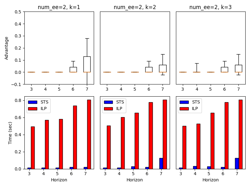
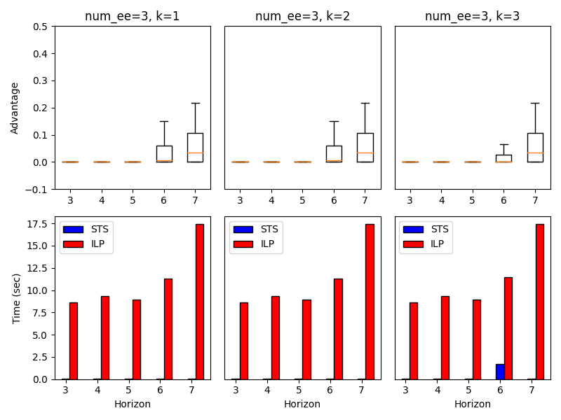
Figure 4: Performance results for synthetic experiments: (Top 2 rows) 2 end-effectors; (Bottom 2 rows) 3 end-effectors. While ILP marginally is better than STS in terms of advantage, STS yields superior speedup over ILP.

4.2 Real World Experiments

We conducted experiments to evaluate the performance of various grasp tool selection algorithms, and to validate the adequacy of the proposed tool changing score in capturing efficiency. First, we compare the MPC-STS with a set of heuristic baselines. Next, we compare the performance of MPC-STS and heuristics baselines against experiments where only a single end-effector was used (no tool changing allowed). We also conduct a series of ablations on MPC-STS in terms of its void radius and max horizon (i.e., $H$). Before we present our results, we first discuss how real-world performance should be best evaluated.

Metric Definitions

Our primary goal is to minimize the cost associated with changing tools, yet still maximize pick success. One way to measure performance is by grasp throughput – the average number of successful picks in a unit time. However, grasp throughput does not correctly penalize strategies that execute many failed grasps quickly, which can be inappropriate for scenarios where items may become damaged as a result of repeated, aggressive picking.

To address this, we propose a combined score based on pick success rate (PSR), and tool consistency rate (TCR), defined as: $\small\mbox{PSR}=\frac{\mbox{PS}}{\mbox{PA}},\hskip 14.45377pt\mbox{TCR}=1-\frac{\mbox{TC}}{\mbox{PA}},$ where PS is the pick success count, PA is the pick attempt count, and TC is the tool change count (here, we do assume that there is no more than one tool change per pick attempt). Ideally, we would like both scores to be high. Also, the PSR and TCR should be balanced according to the time cost of tool change compared to the time cost of a failed grasp. We posit that the following $\beta\text{-}\mbox{TC}\text{-}\mbox{score}$ score captures these desiderata,

$$\small\beta\text{-}\mbox{TC}\text{-}\mbox{score}=\frac{(1+\beta^{2})*\mbox{PSR}*\mbox{TCR}}{\beta^{2}\mbox{PSR}+\mbox{TCR}},$$ (4)

where $\beta$ is analogous to an $F\text{-}beta$ score [BYRN⁺99]. We recommend that $\beta$ be set to the opportunity cost of a single tool change – the approximate number successful picks that could have been completed in the time it takes to execute a tool change. For our setup, we estimated $\beta$ to be $0.33$.

To further motivate the idea behind this metric, we present a simple numerical example that further clarifies the $\beta\text{-}\mbox{TC}\text{-}\mbox{score}$ (see Equation 3, in Real World Experiments in the main paper): consider two tool selection algorithms A, B, being evaluated over a similar scenario (independently) with two items in the bin (i.e., each needs two successful picks to clear the bin):

$$A :T\hskip 1.4457ptF\hskip 1.4457ptF\hskip 1.4457ptF\hskip 1.4457ptS\hskip 1.4457ptT\hskip 1.4457ptS$$

$$B :T\hskip 1.4457ptF\hskip 1.4457ptF\hskip 1.4457ptF\hskip 1.4457ptS\hskip 1.4457ptF\hskip 1.4457ptF\hskip 1.4457ptF\hskip 1.4457ptS$$

In these sequences, T is a tool change event, F is pick fail, and S is pick success. Assume each pick attempt takes 1 second, and each tool change takes 3 seconds. In the above trajectories, both A and B have the same throughput (2 successes per 11 seconds). But we have a preference for A due to less failed pick attempts (A has 3 vs. 6 in B). In each case we have:

$$A :PSR=2/5,TCR=1-2/5=3/5$$

$$B :PSR=2/8,TCR=1-1/8=7/8$$

For small values of $\beta$ (e.g., $\beta<1.0$), TC score places more importance on PSR. For extreme value $\beta=0$, we have TCR = PSR, ignoring the cost of tool change.

For $\beta=0.0$, we are favoring pick success rate:

$$A :\beta\text{-}\mbox{TC}=PSR=0.4$$

$$B :\beta\text{-}\mbox{TC}=PSR=0.25$$

For larger values of $\beta$ (e.g., $\beta>1.0$), TCR gains more importance and in the limit of $\beta=\inf$, we have TC = TCR. In the above example, for $\beta=2$, the TC scores B higher than A.

For $\beta=2$, we are penalizing tool changing more (by letting TCR impact the score more dominantly than PSR):

$$A :\beta\text{-}\mbox{TC}=5*(2/5)*(3/5)/(4*(2/5)+(3/5))=0.545$$

$$B :\beta\text{-}\mbox{TC}=5*(2/8)*(7/8)/(4*(2/8)+(7/8))=0.583$$

As we suggested in the paper, a good balance is obtained when selecting $\beta$ to be the opportunity cost. Here, the overall pick success rate is (2+2)/(5+8) 0.3, and therefore the opportunity cost is slightly less than 1.

For $\beta=1$ we obtain:

$$A :\beta\text{-}\mbox{TC}=2*(2/5)*(3/5)/(1*(2/5)+(3/5))=0.48$$

$$B :\beta\text{-}\mbox{TC}=2*(2/8)*(7/8)/(1*(2/8)+(7/8))=0.39$$

Favoring A, but taking into account the cost of tool swap.

Experimental Setup

We used a Fanuc LRMate 200iD/7L arm, with a tool selection hardware using two vacuum end-effectors: Piab BL30-3P.4L.04AJ (30mm) and Piab BL50-2.10.05AD (50mm). We used an assortment of mixed items (various sizes, weights, shapes, colors, etc., see Figure 1(b) for an example). Each end-effector is associated with a grasp proposal model trained using previously collected production data appropriate for that end-effector. Since it is not in the scope of this paper, we only provide a brief overview of our grasp proposal model architecture. Our grasp proposal models are inspired by the architecture proposed in [GKR20] which consists of encoder-decoder convolutional neural nets consisting of a feature pyramid network [LDG⁺17] on a ResNet-101 backbone and a pixelwise sigmoidal output of volume $W\times H$, where $W\times H$ are the dimensions of the grasp success probabilities $\Gamma_{\mathcal{E}}$. The network is then trained end-to-end using previously collected grasp success/failure data consisting of $\leavevmode\nobreak\ 5k$ grasp data per end-effector using stochastic gradient descent with momentum ($LR=0.0003;p=0.8$). Following the synthetic experiments conclusion, we only used the STS solver.

Comparison with Baselines

Algorithm (w/30mm + 50mm)	TC	PA	PS	TC-Score ($\beta$=0.33)	PS/hr
Randomized	800	2191	744	0.3558	186
Naive Greedy	733	2093	1268	0.6099	317
Greedy	261	2702	1288	0.4999	295.41
MPC-STS	229	2563	1719	0.6885	429.75

Table 1: Performance comparison over different tool selection algorithms. PS/hr is the throughput.

Table 1 compares our method (MPC-STS) with 3 baselines. The first is a randomized selector, which randomly changes tools with probability $p=0.75$ at each step, and forcing a change if not swapped after 10 steps. The second baseline is naive greedy selector, which chooses the next grasp proposal based on one-step reward function (see Equation 1). The third baseline is greedy selector, which accumulates the top $n=5$ likelihood scores for each tool, and selects the tool with the highest sum. Our MPC-STS selector was configured with a void radius of $l=100$mm (roughly $60$ pixels), a maximum of $10$ initial grasp proposal samples per end-effector, sparsity factor $k=2$, and a max horizon of $H=2$ (since it yielded the best results for MPC-STS in this domain based on the ablation results in Table 4). Observe that MPC-STS significantly outperforms the other baselines in terms of both TC-score and pick success rate per hour (improving over the best baseline by $50\%$).

Single end-effector Comparison

This set of comparisons is based on a separate set of shorter experimental runs with similar items; results are reported in Table 2. Here, note the divergence between the TC-score and the throughput (PS/hr) in the ordering of the performance of the single $50$mm end-effector and the naive greedy baseline.

Configuration	TC	PA	PS	TC-Score ($\beta=0.33$)	PS/hr
Single (30mm)	0	745	359	0.508	287.2
Single (50mm)	0	864	572	0.685	490.3
Naive Greedy	217	636	465	0.751	348.8
(30mm + 50mm)
MPC-STS	71	691	524	0.770	507.1
(30mm + 50mm)

Table 2: Comparison of single end-effector performance vs multiple end-effectors and tool selection.

While the throughput for the single $50$mm strategy is higher, the TC-score correctly reflects that this strategy is less pick efficient. Indeed, the successful pick percentage for the $50$mm strategy is  $66\%$ while the successful pick percentage for the naive greedy strategy is  $73\%$. The throughput in this case is inflated by executing failing picks quickly. As expected, MPC-STS outperforms all the baselines.

Parameter Study

In these experiments, reported in Tables 3 and 4, we investigate the dependence on the void radius and max horizon.

MPC-STS (H=3, k=2)	TC	PA	PS	TC-Score ($\beta=0.33$)	PS/hr
l = 50mm	72	720	586	0.822	540.9
l = 100mm	58	649	431	0.682	417.1
l = 150mm	98	619	409	0.675	348.8

Table 3: Investigation of void radius $l$ (in mm).

On our item set, increasing the size of the void radius leads to a decrease in tool-changing efficiency and overall throughput at an MPC-STS with $H=3$. As the tree search progresses, the bin becomes increasingly voided. For large void radii, a large fraction of the bin will be voided, leading to unreliable reward estimates.

Thus, as long as the void radius is large enough to cover areas disturbed by previous picks, the smaller radius the better. We also see that increasing the max horizon $H$ from $1$ to $2$ leads to an increase in performance, but thereafter there is a decrease in performance metrics even though the overall tool change count remains similar.

MPC-STS ($k=2$, $l$=100mm)	TC	PA	PS	TC-Score ($\beta=0.33$)	PS/hr
H = 1	64	712	522	0.747	481.8
H = 2	60	653	511	0.793	502.6
H = 3	58	649	431	0.682	417.1
H = 5	65	646	365	0.586	353.2

Table 4: Investigation of planning horizon.

We conjecture that this is due the crude approximation of the deterministic dynamics, which are not reliable for a long planning horizon.

5 Conclusions and Future Directions

In this work we introduced the Grasp Tool Selection Problem (GTSP), and presented several approximate solutions that can be deployed in real time on realistic robotic setups. Our experiments demonstrated that significant gains can be reaped by carefully planning the tool selection. For industrial bin picking, where every performance gain is directly translated to revenue, we believe that our method could be valuable.

Deep learning based prediction models are becoming increasingly popular in robotics. Our work explored an optimization-based approach for maximizing the utilization of the learned models. In general, we believe that optimally choosing between several learned models could be relevant for other robotic tasks, for example, choosing between different gaits in robotic locomotion. The ideas in this work may inspire algorithms for more general problems.

References

- [Ber12] Dimitri Bertsekas. Dynamic programming and optimal control: Volume I, volume 1. Athena scientific, 2012.
- [BYRN+99] Ricardo Baeza-Yates, Berthier Ribeiro-Neto, et al. Modern information retrieval, volume 463. ACM press New York, 1999.
- [CA13] E. F. Camacho and C. B. Alba. Model predictive control. In Springer Science & Business Media, 2013.
- [DFJ54] George Bernard Dantzig, D. R. Fulkerson, and Selmer Martin Johnson. Solution of a Large-Scale Traveling-Salesman Problem. RAND Corporation, Santa Monica, CA, 1954.
- [EFD+18] Frederik Ebert, Chelsea Finn, Sudeep Dasari, Annie Xie, Alex Lee, and Sergey Levine. Visual foresight: Model-based deep reinforcement learning for vision-based robotic control, 2018.
- [EFLL17] Frederik Ebert, Chelsea Finn, Alex X. Lee, and Sergey Levine. Self-supervised visual planning with temporal skip connections, 2017.
- [FL16] Chelsea Finn and Sergey Levine. Deep visual foresight for planning robot motion. CoRR, abs/1610.00696, 2016.
- [GKR20] Ben Goodrich, Alex Kuefler, and William D. Richards. Depth by poking: Learning to estimate depth from self-supervised grasping. CoRR, abs/2006.08903, 2020.
- [Gur22] Gurobi Optimization, LLC. Gurobi Optimizer Reference Manual, 2022.
- [LDG+17] T. Lin, P. Dollár, R. Girshick, K. He, B. Hariharan, and S. Belongie. Feature pyramid networks for object detection. In 2017 IEEE Conference on Computer Vision and Pattern Recognition (CVPR), pages 936–944, 2017.
- [LLS15] Ian Lenz, Honglak Lee, and Ashutosh Saxena. Deep learning for detecting robotic grasps. The International Journal of Robotics Research, 34(4-5):705–724, 2015.
- [LPKQ16] Sergey Levine, Peter Pastor, Alex Krizhevsky, and Deirdre Quillen. Learning hand-eye coordination for robotic grasping with deep learning and large-scale data collection, 2016.
- [MMS+19] Jeffrey Mahler, Matthew Matl, Vishal Satish, Michael Danielczuk, Bill DeRose, Stephen McKinley, and Ken Goldberg. Learning ambidextrous robot grasping policies. Science Robotics, 4(26), 2019.
- [MTZ60] C.E. Miller, A.W. Tucker, and R.A. Zemlin. Integer programming formulations and traveling salesman problems. Journal of Association for Computing Machinery, 7:326–329, 1960.
- [RA15] Joseph Redmon and Anelia Angelova. Real-time grasp detection using convolutional neural networks, 2015.
- [RN95] Stuart Jonathan Russell and Peter Norvig. Artificial intelligence: A modern approach. 1995.
- [TTZ+16] Aviv Tamar, Garrett Thomas, Tianhao Zhang, Sergey Levine, and Pieter Abbeel. Learning from the hindsight plan - episodic MPC improvement. CoRR, abs/1609.09001, 2016.
- [XELF19] Annie Xie, Frederik Ebert, Sergey Levine, and Chelsea Finn. Improvisation through physical understanding: Using novel objects as tools with visual foresight, 2019.
- [ZSY+18] Andy Zeng, Shuran Song, Kuan-Ting Yu, Elliott Donlon, Francois R Hogan, Maria Bauza, Daolin Ma, Orion Taylor, Melody Liu, Eudald Romo, et al. Robotic pick-and-place of novel objects in clutter with multi-affordance grasping and cross-domain image matching. In 2018 IEEE international conference on robotics and automation (ICRA), pages 3750–3757. IEEE, 2018.