Bandit Social Learning: Exploration under Myopic Behavior

Abstract

We study social learning dynamics motivated by reviews on online platforms. The agents collectively follow a simple multi-armed bandit protocol, but each agent acts myopically, without regards to exploration. We allow a wide range of myopic behaviors that are consistent with (parameterized) confidence intervals for the arms’ expected rewards. We derive stark learning failures for any such behavior, and provide matching positive results. As a special case, we obtain the first general results on failure of the greedy algorithm in bandits, thus providing a theoretical foundation for why bandit algorithms should explore.

1 Introduction

Reviews and ratings are pervasive in many online platforms. A customer consults reviews/ratings, then chooses a product and then (often) leaves feedback, which is aggregated by the platform and served to future customers. Collectively, customers face a tradeoff between exploration and exploitation, i.e., between acquiring new information while making potentially suboptimal decisions and making optimal decisions using available information. However, individual customers tend to act myopically and favor exploitation, without regards to exploration for the sake of the others. On a high level, we ask whether/how the myopic behavior interferes with efficient exploration. We are particularly interested in learning failures when only a few agents choose an optimal action.

Our model. We distill this issue down to its purest form. We posit that the customers make one decision each and do not observe any personalized payoff-relevant information prior to their decision, whether public or private. In particular, the customers believe they are similar to one another. They have only two alternative products/experiences to choose from, a.k.a., arms, and no way to infer anything about one arm from the other. The platform provides each customer with full history on the previous agents.

Concretely, we posit Bandit Social Learning ($\mathtt{BSL}$): a variant of social learning in which the customers (henceforth, agents) follow a simple multi-armed bandit protocol. The agents arrive sequentially. Each agent observes full history, chooses an arm, and receives a reward: a Bernoulli random draw whose mean is specific to this arm and not known to the agents. Initial knowledge — a dataset with some samples of each arm — may be available to all agents. When all agents are governed by a centralized algorithm, this setting is known as stochastic bandits, a standard and well-understood variant of multi-armed bandits.

We allow a wide range of myopic behaviors that are consistent with available observations. Consider standard upper/lower confidence bounds for the reward of each arm: the sample average plus/minus the “confidence term” that scales as a square root of the number of samples. Each agent evaluates each arm to an index: some number that is consistent with these confidence bounds (but could be arbitrary otherwise), and chooses an arm with a largest index. The confidence term is parameterized by some factor $\sqrt{\eta}\geq 0$ to ensure that the true mean reward lies between the confidence bounds with probability at least $1-e^{-2\eta}$. We call such agents $\eta$-confident. We emphasize that $\eta$ is a parameter of the model, rather than something that can be adjusted.

This model subsumes the “unbiased” behavior, when the index equals the sample average, as well as “optimism” and “pessimism”, when the index is, resp., larger or smaller than the sample average. Such optimism/pessimism can also be interpreted as risk preferences. The index can be randomized, so that the less preferred arm is chosen with a smaller, but strictly positive probability. Further, an agent may be more optimistic about one arm than the other, and the exact amount of optimism / pessimism may depend on the previously observed rewards of either arm, and even favor more recent observations. Finally, different agents may exhibit different behaviours within the permitted range. (We discuss these behaviors more in Related Work and Section 2.1.)

We target the regime when parameter $\eta$ is a constant relative to $T$, the number of agents, i.e., the agents’ population is characterized by a constant $\eta$. We are interested in the asymptotic behavior when $T$ increases.

An extreme version of our model, with $\eta\sim\log(T)$, is only considered for intuition and sanity checks. Interestingly, this extreme version subsumes two well-known bandit algorithms: UCB1 (Auer et al., 2002a) and Thompson Sampling (Thompson, 1933; Russo et al., 2018), which achieve optimal regret bounds. These algorithms exemplify standard design paradigms – resp., optimism under uncertainty and posterior sampling – which usefully extend to many scenarios in bandits and reinforcement learning. They can also be seen as behaviors: resp., extreme optimism and probability matching (Myers, 1976; Vulkan, 2000), a well-known randomized behavior. More “moderate” versions of these behaviors are consistent with $\eta$-confidence as defined above, and are subject to the learning failures described below.

Mean rewards	Beliefs	Behavior	Results
fixed	“frequentist”	$\eta$-confident	Thm. 3.2 (main),
	confidence intervals		Thm. 3.11 (small $N_{0}$).
		unbiased/Greedy	Cor. 3.8
		$\eta_{t}$-pessimistic	Thm. 3.12
	Bayesian (independent)	Bayesian-unbiased	Thm. 5.1(a)
		$\eta$-Bayesian-confident	Thm. 5.1(b)
Bayesian (correlated)	Bayesian (and correct)	Bayesian-unbiased	Thm. 6.1; Cor. 6.2, 6.4

Table 1: Our negative results: learning failures.

Our results. We are interested in learning failures when all but a few agents choose the bad arm, and how the failure probability scales with the $\eta$ parameter.

Our main result is that if all agents are $\eta$-confident, the failure probability is at least $e^{-O(\eta)}$ (see Section 3). Consequently, regret is at least $\Omega(T\cdot e^{-O(\eta)})$ for any given problem instance, in contrast with the $O(\log T)$ regret rate obtained by optimal bandit algorithms. Further, the $e^{-O(\eta)}$ scaling is the best possible: indeed, regret for optimistic agents is at most $O\left(\,T\cdot e^{-\Omega(\eta)}+\eta\,\right)$ for a given problem instance (Theorem 4.1). Note that the negative result deteriorates as $\eta$ increases, and becomes vacuous when $\eta\sim\log T$; the upper bound then essentially matches the optimal $O(\log T)$ regret of the UCB algorithm Auer et al. (2002a)).

We refine these results in several directions:

• If all agents are “unbiased”, the failure probability scales as the difference in expected reward between the two arms (Corollary 3.8).

• If all agents are pessimistic, then any level of pessimism, whether small or large or different across agents, leads to the similar failure probability as in the unbiased case (Theorem 3.12).

• A small fraction of optimists goes a long way! If all agents are $\eta$-confident and even a $q$-fraction of them are $\eta$-optimistic, this yields regret $O\left(\,T\cdot e^{-\Omega(\eta)}+\eta/q\,\right)$.

Our results extend to Bayesian agents who have beliefs (i.e., Bayesian priors) and act according to their posteriors. When agents’ beliefs are independent across arms and expressed by Beta distributions, such agents are consistent with our main model of $\eta$-confident agents, and therefore are subject to the same negative results (Section 5). Further, we focus on Bayesian-unbiased agents and allow arbitrary correlated Bayesian beliefs, when the agents can make inferences about one arm from the observations on the other (Section 6). We derive a general result on learning failures, assuming that the mean rewards are actually drawn according to the beliefs .

Our results are summarized in Tables 1 and 2. Further, we extend our negative results to $K\geq 2$ arms (Section 7) and provide some numerical simulations to illustrate our key findings (Section 8).

Mean rewards	Beliefs	Behavior	Result
fixed	“frequentist”	$\eta$-optimistic	Thm. 4.1
	confidence	$\eta_{t}$-optimistic, $\eta_{t}\in[\eta,\eta_{\max}]$	Thm. 4.4
	intervals	small fraction of optimists	Thm. 4.5

Table 2: Our positive results: upper bounds on regret.

Implications for multi-armed bandits. The negative results for unbiased agents can be seen as general results on the failure of the greedy algorithm: a bandit algorithm that always exploits. This is a theoretical foundation for why bandit algorithms should explore – and indeed why one should design them. We are not aware of any general results of this nature, whether published or known previously as ”folklore”. This is quite surprising given the enormous literature on multi-armed bandits. Therefore, we believe our results fill an important gap in this literature.

How surprising are these results? It has been folklore knowledge for several decades that the greedy algorithm is inefficient in some simple special cases, and folklore belief that this should hold much more generally. However, recent results reveal a more complex picture: the greedy algorithm fails under some strong assumptions, but works well under some other strong assumptions (see Related Work). Thus, it has arguably became less clear which assumptions would be needed for negative results and what would be the “shape” and probability of learning failures.

Further, our results on $\eta$-confident agents explain why UCB1 algorithm requires extreme optimism, why any algorithm based on narrow (constant-$\eta$) confidence intervals is doomed to fail, and also why “pessimism under uncertainty” is not a productive approach for exploration.

Novelty and significance. $\mathtt{BSL}$ was not well-understood previously even with unbiased agents, as discussed above, let alone for more permissive behavioral models. It was very unclear a priori how to analyze learning failures and how strong would be the guarantees, in terms of the generality of agents’ behaviors, the failure events/probabilities, and the technical assumptions.

On a technical level, our proofs have very little (if anything) to do with standard lower-bound analyses in bandits stemming from Lai and Robbins (1985) and Auer et al. (2002b). These analysis apply any algorithm and prove “sublinear” lower bounds on regret, such as $\Omega(\log T)$ for a given problem instance and $\Omega(\sqrt{T})$ in the worst case. Their main technical tool is KL-divergence analysis showing that no algorithm can distinguish between a given tuple of ”similar” problem instances. In contrast, we prove linear lower bounds on regret, our results apply to a particular family of behaviors/algorithms, and we never consider a tuple of similar problem instances. Instead, we use anti-concentration and martingale tools to argue that the best arm is never played (or played only a few times), with some probability. While the tools themselves are not very standard, the novelty is primarily in how we use these tools. The result on correlated beliefs in Section 6 has a rather short but ”conceptual” proof which we believe is well-suited for a textbook.

While our positive results in Section 4 are restricted to “optimistic” agents, we do not assert that such agents are necessarily typical. The primary point here is that our results on learning failures are essentially tight. That said, “optimism” is a well-documented behavioral bias (e.g., see (Puri and Robinson, 2007) and references therein). So, a small fraction of optimists (leveraged in Theorem 4.5) is not unrealistic.

Our proofs are more involved compared to the standard analysis of the UCB1 algorithm. This is because we cannot make the $\eta$ parameter as large as needed to ensure that the complements of certain “clean events” can be ignored. Instead, we need to define and analyze these “clean events” in a more careful way. These difficulties are compounded in Theorem 4.5, our most general result. As far as the statements are concerned, the basic result in Theorem 4.1 is perhaps what one would expect to hold, whereas the extensions in Theorem 4.4 and Theorem 4.5 are more surprising.

Framing. We target the scenario in social learning when both actions and rewards are observable in the future, and the agents do not receive any other payoff-relevant signals. The primary goal is to analyze the learning behavior of a system of agents (rather than design an algorithm or a mechanism). As in much of algorithmic game theory, we discuss the influence of self-interested behavior on the overall welfare of the system. We consider how such behaviour can cause “learning failures”, which is a typical framing in the literature on social learning. From the perspective of multi-armed bandits, we investigate the failures of the greedy algorithm, and more generally any algorithm that operates on narrow confidence intervals. We do not attempt to design new algorithms, as a version of UCB1 is proved optimal.

Map of the paper. Section 2 introduces our model in detail and discusses various allowed behaviors. Section 3 derives the learning failures. Section 4 presents our positive results. Section 5 and Section 6 handle agents with Bayesian beliefs. Negative results for $K\geq 2$ arms are Section 7. Numerical simulations are in Section 8. Some unessential proofs are moved to appendices.

1.1 Related Work

Social learning. A vast literature on social learning studies agents that learn over time in a shared environment. A prominent topic is the presence or absence of learning failures such as ours. Models vary across several dimensions, such as: which information is acquired or transmitted, what is the communication network, whether agents are long-lived or only act once, how they choose their actions, etc. All models from prior work are very different from ours. Below we separate our model from several lines of work that are most relevant.

In “sequential social learning”, starting from (Banerjee, 1992; Welch, 1992; Bikhchandani et al., 1992; Smith and Sørensen, 2000), agents observe private signals, but only the chosen actions are observable in the future; see Golub and Sadler (2016) for a survey. The social planner (who chooses agents’ actions given access to the knowledge of all previous agents) only needs to exploit, i.e., choose the best action given the previous agents’ signals, whereas in our model it also needs to explore. Learning failures are (also) of primary interest, but they occur for an entirely different reason: restricted information flow, since the private signals are not observable in the future.

“Strategic experimentation”, starting from Bolton and Harris (1999) and Keller et al. (2005), studies long-lived learning agents that observe both actions and rewards of one another; see Hörner and Skrzypacz (2017) for a survey. Here, the social planner also solves a version of multi-armed bandits, albeit a very different one (with time-discounting, “safe” arm that is completely known, and “risky” arm that follows a stochastic process). The main difference is that the agents engage in a complex repeated game where they explore but prefer to free-ride on exploration by others.

Bala and Goyal (1998) and Lazer and Friedman (2007) consider a network of myopic learners, all faced with the same bandit problem and observing each other’s actions and rewards. The interaction protocol is very different from ours: agents are long-lived, act all at once, and only observe their neighbors on the network. Other specifics are different, too. Bala and Goyal (1998) makes strong assumptions on learners’ beliefs, which would essentially cause the greedy algorithm to work well in $\mathtt{BSL}$. In Lazer and Friedman (2007), each learner only retains the best observed action, rather than the full history. The focus is on comparing the impact of different network topologies, theoretically (Bala and Goyal, 1998) and via simulations (Lazer and Friedman, 2007).

Prominent recent work, e.g., (Heidhues et al., 2018; Bohren and Hauser, 2021; Fudenberg et al., 2021; Lanzani, 2023), targets agents with misspecified beliefs, i.e., beliefs whose support does not include the correct model. The framing is similar to $\mathtt{BSL}$ with Bayesian-unbiased agents: agents arrive one by one and face the same decision problem, whereby each agent makes a rational decision after observing the outcomes of the previous agents. Rational decisions under misspecified beliefs make a big difference compared to $\mathtt{BSL}$, and structural assumptions about rewards/observations and the state space tend to be very different from ours. The technical questions being asked tend to be different, too. E.g., convergence of beliefs is of primary interest, whereas the chosen arms and agents’ beliefs/estimates trivially converge in our setting.

The greedy algorithm. Positive results for the greedy bandit algorithm focus on contextual bandits, an extension of stochastic bandits where a payoff-relevant signal (context) is available before each round. Equivalently, this is a version of $\mathtt{BSL}$ where each agent observes an idiosyncratic signal along with the history, and the signals are public, i.e., visible to the future agents. The greedy algorithm has been proved to work well under very strong assumptions on the primitives of the economic environment: linearity of rewards and diversity of contexts (Kannan et al., 2018; Bastani et al., 2021; Raghavan et al., 2023). Acemoglu et al. (2022) obtain similar results for $\mathtt{BSL}$ with private signals (i.e., not visible to the future agents), under different (and also very strong) assumptions on structure and diversity. In all this work, agents’ diversity substitutes for exploration, and structural assumptions allow aggregation across agents. We focus on a more basic model, where this channel is ruled out.

The greedy algorithm is also known to attain $o(T)$ regret in various scenarios with a very large number of near-optimal arms (Bayati et al., 2020; Jedor et al., 2021), e.g., for Bayesian bandits with $\gg\sqrt{T}$ arms, where the arms’ mean rewards are sampled independently and uniformly.

Learning failures for the greedy algorithm are derived for bandit problems with 1-dimensional action spaces under (strong) structural assumptions: e.g., dynamic pricing with linear demands (Harrison et al., 2012; den Boer and Zwart, 2014) and dynamic control in a (generalized) linear model (Lai and Robbins, 1982; Keskin and Zeevi, 2018). In all these results, the failure probability is only proved positive, but not otherwise characterized. The greedy algorithm is restricted to one or two initial samples (which is a trivial case in our setting, as per Footnote 8).

$\mathtt{BSL}$ and mechanism design. Incentivized exploration takes a mechanism design perspective on $\mathtt{BSL}$, whereby the platform strives to incentivize individual agents to explore for the sake of the common good. In most of this work, starting from (Kremer et al., 2014; Che and Hörner, 2018), the platform controls the information flow, e.g., can withhold history and instead issue recommendations, and uses this information asymmetry to create incentives; surveys can be found in (Slivkins, 2023) and (Slivkins, 2019, Ch. 11). In particular, (Mansour et al., 2020; Immorlica et al., 2020; Sellke and Slivkins, 2022) target stochastic bandits as the underlying learning problem, same as we do. Most related is Immorlica et al. (2020), where the platform constructs a (very) particular communication network for the agents, and then the agents engage in $\mathtt{BSL}$ on this network.

Alternatively, the agents are allowed to observe full history, but the platform uses monetary payments to create incentives (Frazier et al., 2014; Han et al., 2015; Chen et al., 2018). The platform’s goal is to optimize the welfare vs. payments tradeoff under time-discounting.

Behaviorial models. Non-Bayesian models of behavior are prominent in the literature on social learning, starting from DeGroot (1974). In these models, agents use variants of statistical inference and/or naive rules-of-thumb to infer the state of the world from observations. In particular, our model of $\eta$-confident agents is essentially a special case of “case-based decision theory” of Gilboa and Schmeidler (1995).

Our model accommodates versions of several behaviorial biases:

• optimism (e.g., see (Puri and Robinson, 2007) and references therein),

• pessimism (e.g., see (Chang, 2000; Bateson, 2016) and references therein),

• risk attitudes (e.g., see (Kahneman and Tversky, 1982; Barberis and Thaler, 2003)),

• recency bias (e.g., see (Fudenberg and Levine, 2014) and references therein),

• randomized decisions (with theory tracing back to Luce (1959)), and

• probability matching more specifically (e.g., see surveys (Myers, 1976; Vulkan, 2000)).

All these biases are well-documented and well-studied in the literature on economics and psychology. A technical discussion of how these and other behaviors fit into our model is in Section 2.1.

Multi-armed bandits. Our perspective of multi-armed bandits is very standard in machine learning theory: we consider asymptotic regret rates without time-discounting (rather than Bayesian-optimal time-discounted rewards, a more standard economic perspective). The vast literature on regret-minimizing bandits is summarized in books (Bubeck and Cesa-Bianchi, 2012; Slivkins, 2019; Lattimore and Szepesvári, 2020).

Stochastic bandits is a standard, basic version with i.i.d. rewards and no auxiliary structure. Most relevant are the UCB1 algorithm (Auer et al., 2002a), Thompson Sampling and the “frequentist” analyses thereof (Thompson, 1933; Russo et al., 2018; Agrawal and Goyal, 2012a, 2017; Kaufmann et al., 2012), and the lower bounds (e.g.,  Lai and Robbins, 1985; Auer et al., 2002b). The general design paradigms associated with UCB1 and Thompson Sampling are surveyed in (Bubeck and Cesa-Bianchi, 2012; Slivkins, 2019; Lattimore and Szepesvári, 2020; Russo et al., 2018).

Markovian, time-discounted bandit formulations (Gittins et al., 2011; Bergemann and Välimäki, 2006) and various other connections between bandits and self-interested behavior (surveyed, e.g., in Slivkins (2019, Chapter 11.7)) are less relevant to this paper.

2 Our model and preliminaries

Our model, called Bandit Social Learning, is defined as follows. There are $T$ rounds, where $T\in\mathbb{N}$ is the time horizon, and two arms (i.e., alternative actions). We use $[T]$ and $[2]$ to denote the set of rounds and arms, respectively. In each round $t\in[T]$, a new agent arrives, observes history $\mathtt{hist}_{t}$ (defined below), chooses an arm $a_{t}\in[2]$, receives reward $r_{t}\in[0,1]$ for this arm, and leaves forever. When a given arm $a\in[2]$ is chosen, its reward is drawn independently from Bernoulli distribution with mean $\mu_{a}\in[0,1]$. The mean reward is fixed over time, but not known to the agents. Some initial data is available to all agents, namely $N_{0}\geq 1$ samples of each arm $a\in[2]$. We denote them $r^{0}_{a,i}\in[0,1]$, $i\in[N_{0}]$. The history in round $t$ consists of both the initial data and the data generated by the previous agents. Formally, it is a tuple of arm-reward pairs,

$$\mathtt{hist}_{t}:=\left(\,(a,r^{0}_{a,i}):\;a\in[2],i\in[N_{0}];\;(a_{s},r_{s}):\;s\in[t-1]\,\right).$$

We summarize the protocol for Bandit Social Learning as Protocol 1.

Problem instance: two arms $a\in[2]$ with (fixed, but unknown) mean rewards $\mu_{1},\mu_{2}\in[0,1]$ ;

Initialization: $\mathtt{hist}\leftarrow\left\{\,\text{$N_{0}$ samples of each arm}\,\right\}$;

for each round $t=1,2,\ldots,T$ do

       agent $t$ arrives, observes $\mathtt{hist}$ and chooses an arm $a_{t}\in[2]$ ;

       reward $r_{t}\in\left[\,0,1\,\right]$ is drawn from Bernoulli distribution with mean $\mu_{a_{t}}$;

       new datapoint $(a_{t},r_{t})$ is added to $\mathtt{hist}$

Protocol 1 Bandit Social Learning

Remark 2.1.

The initial data-points represent reports created outside of our model, e.g., by ghost shoppers, influencers, paid reviewers, journalists, etc., and available before (or soon after) the products enter the market. While the actual reports may have a different format, they shape agents’ initial beliefs. So, one could interpret our initial data-points as a simple “frequentist” representation for the initial beliefs. Accordingly, parameter $N_{0}$ determines the “strength” of the beliefs. We posit $N_{0}\geq 1$ to ensure that the arms’ average rewards are always well-defined.

If the agents were controlled by an algorithm, this protocol would correspond to stochastic bandits with two arms, the most basic version of multi-armed bandits. A standard performance measure in multi-armed bandits (and online machine learning more generally) is regret, defined as

$$\textnormal{Regret}(T)\mathrel{:=}\textstyle\mu^{*}\cdot T-{\mathbb{E}\left[\,\sum_{t\in[T]}\;\mu_{a_{t}}\,\right]},$$ (2.1)

where $\mu^{*}=\max(\mu_{1},\mu_{2})$ is the maximal expected reward of an arm.

Each agent $t$ chooses its arm $a_{t}$ myopically, without regard to future agents. Each agent is endowed with some (possibly randomized) mapping from histories to arms, and chooses an arm accordingly. This mapping, called behavioral type, encapsulates how the agent resolves uncertainty on the rewards. More concretely, each agent maps the observed history $\mathtt{hist}_{t}$ to an index $\mathtt{Ind}_{a,t}\in\mathbb{R}$ for each arm $a\in[2]$, and chooses an arm with a largest index. The ties are broken independently and uniformly at random.

We allow for a range of myopic behaviors, whereby each index can take an arbitrary value in the (parameterized) confidence interval for the corresponding arm. Formally, fix arm $a\in[2]$ and round $t\in[T]$. Let $n_{a,t}$ denote the number of times this arm has been chosen in the history $\mathtt{hist}_{t}$ (including the initial data), and let ${\hat{\mu}}_{a,t}$ denote the corresponding average reward. Given these samples, standard (frequentist, truncated) upper and lower confidence bounds for the arm’s mean reward $\mu_{a}$ (UCB and LCB, for short) are defined as follows:

$$\mathtt{UCB}^{\eta}_{a,t}:=\min\left\{\,1,{\hat{\mu}}_{a,t}+\sqrt{\eta/n_{a,t}}\,\right\}\quad\text{and}\quad\mathtt{LCB}^{\eta}_{a,t}:=\max\left\{\,0,{\hat{\mu}}_{a,t}-\sqrt{\eta/n_{a,t}}\,\right\},$$ (2.2)

where $\eta\geq 0$ is a parameter. The interval $\left[\,\mathtt{LCB}^{\eta}_{a,t},\mathtt{UCB}^{\eta}_{a,t}\,\right]$ will be referred to as $\eta$-confidence interval. Standard concentration inequalities imply that $\mu_{a}$ is contained in this interval with probability at least $1-2\,e^{-2\eta}$ (where the probability is over the random rewards, for any fixed value of $\mu_{a}$). We allow the index to take an arbitrary value in this interval:

$$\mathtt{Ind}_{a,t}\in\left[\,\mathtt{LCB}^{\eta}_{a,t},\mathtt{UCB}^{\eta}_{a,t}\,\right],\quad\text{for each arm $a\in[2]$}.$$ (2.3)

We refer to such agents as $\eta$-confident; $\eta>0$ will be a crucial parameter throughout.

We posit that the agents come from some population characterized by some fixed $\eta$, while the number of agents ($T$) can grow arbitrarily large. Thus, we are mainly interested in the regime when $\eta$ is a constant with respect to $T$.

2.1 Special cases of our model

We emphasize the following special cases of $\eta$-confident agents:

• unbiased agents set each index to the respective sample average: $\mathtt{Ind}_{a,t}={\hat{\mu}}_{a,t}$. This is a natural myopic behavior for a “frequentist” agent in the absence of behavioral biases.

• $\eta$-optimistic agents evaluate the uncertainty on each arm in the optimistic way, setting the index to the corresponding UCB: $\mathtt{Ind}_{a,t}=\mathtt{UCB}^{\eta}_{a,t}$.

• $\eta$-pessimistic agents exhibit pessimism, in the same sense: $\mathtt{Ind}_{a,t}=\mathtt{LCB}^{\eta}_{a,t}$.

Unbiased agents correspond precisely to the greedy algorithm in multi-armed bandits which is entirely driven by exploitation, and chooses arms as $a_{t}\in\operatorname*{argmax}_{a\in[2]}{\hat{\mu}}_{a,t}$. In contrast, $\eta$-optimistic agents with $\eta\sim\log T$ correspond to UCB1 (Auer et al., 2002a), a standard algorithm for stochastic bandits which achieves optimal regret rates. We interpret such agents as exhibiting extreme optimism, in that $\mathtt{Ind}_{a,t}\geq\mu_{a}$ with very high probability. Meanwhile, our model focuses on (more) moderate amounts of optimism, whereby $\eta$ is a constant with respect to $T$.

Other behavioral biases. One possible interpretation for $\mathtt{Ind}_{a,t}$ is that it can be seen as certainty equivalent, i.e., the smallest reward that agent $t$ is willing to take for sure instead of choosing arm $a$. Then $\eta$-optimism and $\eta$-pessimism corresponds to (moderate) risk-seeking and risk-aversion, respectively. In particular, $\eta$-pessimistic agents may be quite common.

Our model also accommodates a version of recency bias, whereby recent observations are given more weight. For example, an $\eta$-confident agent may be $\eta$-optimistic for a given arm if more recent rewards from this arm are better than the earlier ones.

An $\eta$-confident agent could have a preference towards a given arm $a$, and therefore, e.g., be $\eta$-optimistic for this arm and $\eta$-pessimistic for the other arm. The agent’s “attitude” towards arm $a$ could also be influenced by the rewards of the other arm, e.g., (s)he could be $\eta$-optimistic for arm $a$ if the rewards from the other arms are high.

Randomized agents. Our model also accommodates randomized $\eta$-confident agents, i.e., ones that draw their indices from some distribution conditional on the history $\mathtt{hist}_{t}$. Such randomization is consistent with a well-known type of behaviors when human agents choose a seemingly inferior alternative with smaller but non-zero probability.

A notable special case is related to probability matching, when the probability of choosing an arm equals to the (perceived) probability of this arm being the best. We formalize this case in a Bayesian framework, whereby all agents have a Bayesian prior such that the mean reward $\mu_{a}$ for each arm $a$ is drawn independently from the uniform distribution over $[0,1]$. Each agent $t$ computes the Bayesian posterior ${\mathcal{P}}_{a,t}$ on $\mu_{a}$ given the history $\mathtt{hist}_{t}$, then samples a number $\nu_{a,t}$ independently from this posterior. Finally, we define each index $\mathtt{Ind}_{a,t}$, $a\in[2]$ as the “projection” of $\nu_{a,t}$ into the corresponding $\eta$-confidence interval $\left[\,\mathtt{LCB}^{\eta}_{a,t},\mathtt{UCB}^{\eta}_{a,t}\,\right]$. Here, the projection of a number $x$ into an interval $[a,b]$ is defined as $a$ if $x<a$, $b$ if $x>b$, and $x$ otherwise.

Here’s why this construction is interesting. Without truncation, i.e., when $\mathtt{Ind}_{a,t}=\nu_{a,t}$, each arm is chosen precisely with probability of this arm being the best according to the posterior $\left(\,{\mathcal{P}}_{1,t},\,{\mathcal{P}}_{2,t}\,\right)$. In fact, this behavior precisely corresponds to Thompson Sampling (Thompson, 1933), another standard multi-armed bandit algorithm that attains optimal regret. For $\eta\sim\log T$, the system of agents behaves like Thompson Sampling with very high probability; we interpret such behavior as an extreme version of probability matching. Meanwhile, we focus on moderate regimes such that $\eta$ is a constant with respect to $T$. We refer to such agents as $\eta$-Thompson agents.

Let us flag two other randomized behaviors allowed by our model. First, a naive form of probability matching chooses an index of each arm independently and uniformly at random from the respective $\eta$-confidence interval. This is one way to express complete uncertainty on which values within each confidence interval are more likely. Second, an even more naive decision rule chooses an arm uniformly at random if the two $\eta$-confidence intervals overlap. Incidentally, this is active arms elimination (Even-Dar et al., 2006), a well-known (and regret-optimal) algorithm for multi-armed bandits. Both behaviors provide stylized reference points for how “naive” human agents may behave in practice.

Bayesian agents. We also accommodate agents that preprocess the observed data to a Bayesian posterior, and use the latter to define their indices; we term them Bayesian agents. We analyze Bayesian versions of unbiased agents and $\eta$-confident agents, interpreting them as (frequentist) $\eta^{\prime}$-confident agents defined above (with slightly larger parameter $\eta^{\prime}$). We restrict our analysis to Beta distributions that are independent across arms. The details are in Section 5.

2.2 Preliminaries

Reward-tape. It is convenient for our analyses to interpret the realized rewards of each arm as if they are written out in advance on a “tape”. We posit a matrix $\left(\,\mathtt{Tape}_{a,i}\in[0,1]:\;a\in[2],\;i\in[T]\,\right)$, called reward-tape, such that each entry $\mathtt{Tape}_{a,i}$ is an independent Bernoulli draw with mean $\mu_{a}$. This entry is returned as reward when and if arm $a$ is chosen for the $i$-th time. (We start counting from the initial samples, which comprise entries $i\in[N_{0}]$.) This is an equivalent (and well-known) representation of rewards in stochastic bandits.

We will use the notation for the UCBs/LCBs defined by the reward-tape. Fix arm $a\in[2]$ and $n\in[T]$. Let $\widehat{\mu}^{\mathtt{tape}}_{a,n}=\tfrac{1}{n}\sum_{i\in[n]}\mathtt{Tape}_{a,i}$ be the average over the first $n$ entries for arm $a$. Now, given $\eta\geq 0$, define the appropriate confidence bounds:

$$\mathtt{UCB}^{\mathtt{tape},\,\eta}_{a,n}:=\min\left\{\,1,\widehat{\mu}^{\mathtt{tape}}_{a,n}+\sqrt{\eta/n}\,\right\}\quad\text{and}\quad\mathtt{LCB}^{\mathtt{tape},\,\eta}_{a,n}:=\max\left\{\,0,\widehat{\mu}^{\mathtt{tape}}_{a,n}-\sqrt{\eta/n}\,\right\}.$$ (2.4)

Good/bad arm. When $\mu_{1},\mu_{2}$ are fixed (rather than drawn from a prior), we posit that $\mu_{1}>\mu_{2}$. That is, arm $1$ is the good arm, and arm $2$ is the bad arm. Our guarantees depend on $\Delta:=\mu_{1}-\mu_{2}$, called the gap (between the two arms), a very standard quantity in multi-armed bandits.

The big-O notation. We use the big-O notation to hide constant factors. Specifically, $O(X)$ and $\Omega(X)$ mean, resp., “at most $c_{0}\cdot X$” and “at least $c_{0}\cdot X$” for some absolute constant $c_{0}>0$ that is not specified in the paper. When and if $c_{0}$ depends on some other absolute constant $c$ that we specify explicitly, we point this out in words and/or by writing, resp., $O_{c}(X)$ and $\Omega_{c}(X)$.

Bandit algorithms. Algorithms UCB1 and Thompson Sampling achieve regret

$$\textnormal{Regret}(T)\leq O\left(\,\min\left(\,1/\Delta,\sqrt{T}\,\right)\cdot\log T\,\right).$$ (2.5)

This regret rate is essentially optimal among all bandit algorithms: it is optimal up to constant factors for fixed $\Delta>0$, and up to $O(\log T)$ factors for fixed $T$ (see Section 1.1 for citations).

A key property of a reasonable bandit algorithm is that $\textnormal{Regret}(T)/T\to 0$; this property is also called no-regret. Conversely, algorithms with $\textnormal{Regret}(T)\geq\Omega(T)$ are considered very inefficient.

A bandit algorithm implemented by a collective of $\eta$-confident agents will be called an $\eta$-confident algorithm. Likewise, $\eta$-optimistic algorithm and $\eta$-pessimistic algorithm.

3 Learning failures

In this section, we prove that the agents’ myopic behavior causes learning failures, i.e., all but a few agents choose the bad arm. More precisely:

Definition 3.1.

The $n$-sampling failure is an event that all but $\leq n$ agents choose the bad arm.

Our main result allows arbitrary $\eta$-confident agents. Essentially, it asserts that $0$-sampling failures happen with probability at least $p_{\mathtt{fail}}\sim e^{-O(\eta)}$. This is a stark learning failure when $\eta$ is a constant relative to the time horizon $T$.

We make two technical assumptions:

$$\text{arms' mean rewards lie in $(c,1-c)$, for some absolute constant $c\in(0,\nicefrac{{1}}{{2}})$},$$ (3.1)

$$\text{the number of initial samples satisfies $N_{0}\geq 64\,\eta/c^{2}+1/c$}.$$ (3.2)

The meaning of (3.1) is that it rules out degenerate behaviors when mean rewards are close to the known upper/lower bounds. The big-O notation hides the dependence on the absolute constant $c$, when and if explicitly stated so. Assumption (3.2) ensures that the $\eta$-confidence interval is a proper subset of $[0,1]$ for all agents; we sidestep this assumption later in Theorem 3.11.

Thus, the result is stated as follows:

Theorem 3.2 ($\eta$-confident agents).

Suppose all agents are $\eta$-confident, for some fixed $\eta\geq 0$. Make assumptions (3.1) and (3.2). Then the $0$-sampling failure occurs with probability at least

$$p_{\mathtt{fail}}=\Omega_{c}\left(\,\sqrt{(1+\eta)/N_{0}}\,\right)\cdot e^{-O_{c}\left(\,\eta\;+\;N_{0}\Delta^{2}\,\right)},\quad\text{where}\quad\Delta=\mu_{1}-\mu_{2}.$$ (3.3)

Consequently, $\textnormal{Regret}(T)\geq\Delta\cdot p_{\mathtt{fail}}\cdot T$.

Discussion 3.3.

The agents in Theorem 3.2 can exhibit any behaviors, possibly different for different agents and different arms, as long as these behaviors are consistent with the $\eta$-confidence property. In particular, this result applies to deterministic behaviours such as optimism/pessimism, and also to randomized behaviors such as $\eta$-Thompson agents defined in Section 2.1.

From the perspective of multi-armed bandits, Theorem 3.2 implies that $\eta$-confident bandit algorithms with constant $\eta$ cannot be no-regret, i.e., cannot have regret sublinear in $T$.

Note that the guarantee in Theorem 3.2 deteriorates as the parameter $\eta$ increases, and becomes essentially vacuous when $\eta\sim\log(T)$. The latter makes sense, since this regime of $\eta$ is used in UCB1 algorithm and suffices for Thompson Sampling.

Discussion 3.4.

Assumption (3.2) is innocuous from the social learning perspective: essentially, the agents hold initial beliefs grounded in data and these beliefs are not completely uninformed. From the bandit perspective, this assumption is less innocuous: while it seems unreasonable to discard the initial data, an algorithm can always choose to do so, possibly side-stepping the failure result. In any case, we remove this assumption in Theorem 3.11 below.

Remark 3.5.

A weaker version of (3.2), namely $N_{0}\geq\eta$, is necessary to guarantee an $n$-sampling failure for any $\eta$-confident agents. Indeed, suppose all agents are $\eta$-optimistic for arm $1$ (the good arm), and $\eta$-pessimistic for arm $2$ (the bad arm). If $N_{0}<\eta$, then the index for arm $2$ is $0$ after the initial samples, whereas the index of arm $1$ is always positive. Then all agents choose arm $1$.

Next, we spell out two corollaries which help elucidate the main result.

Corollary 3.6.

If the gap is sufficiently small, $\Delta<O\left(\,1/\sqrt{N_{0}}\,\right)$, then Theorem 3.2 holds with

$$p_{\mathtt{fail}}=\Omega_{c}\left(\,\sqrt{(1+\eta)/N_{0}}\,\right)\cdot e^{-O_{c}(\eta)}.$$ (3.4)

Remark 3.7.

The assumption in Corollary 3.6 is quite mild in light of the fact that when $\Delta>\Omega\left(\,\sqrt{\log(T)/N_{0}}\,\right)$, the initial samples suffice to determine the best arm with high probability.

Corollary 3.8.

If all agents are unbiased, then Theorem 3.2 holds with $\eta=0$ and

$$p_{\mathtt{fail}} =\Omega_{c}\left(\,1/\sqrt{N_{0}}\,\right)\cdot e^{-O_{c}\left(\,N_{0}\;\Delta^{2}\,\right)}$$ (3.5)

$$=\Omega_{c}\left(\,1/\sqrt{N_{0}}\,\right)\qquad\qquad\text{if $\Delta<O\left(\,1/\sqrt{N_{0}}\,\right)$}.$$

In the latter case, $\textnormal{Regret}(T)\geq\Omega_{c}\left(\,\Delta/\sqrt{N_{0}}\,\right)\cdot T$.

Remark 3.9.

A trivial failure result for unbiased agents relies on the event ${\mathcal{E}}$ that all $N_{0}$ initial samples of the good arm are realized as $0$. (${\mathcal{E}}$ implies a $0$-sampling failure as long as $\geq 1$ initial sample of the bad arm is realized to $1$.) This result is weak for $N_{0}\gg 1$ since ${\mathrm{Pr}\left[\,{\mathcal{E}}\,\right]}=(1-\mu_{1})^{N_{0}}$. In contrast, our guarantee on the failure probability scales as $1/\sqrt{N_{0}}$ when the gap is small enough.

Discussion 3.10.

Corollary 3.8 can be seen as a general result on the failure of the greedy algorithm. This is the first such result with a non-trivial dependence on $N_{0}$, to the best of our knowledge.

Let us remove assumption (3.2) and allow “small” $N_{0}$, namely $N_{0}\leq N_{*}:=\lceil 64\eta/c^{2}+1/c\rceil$. While the analysis of initial samples simplifies — we rely on all samples being $0$ for the good arm and $1$ for the bad arm — the rest of the analysis becomes more intricate. Essentially, this is due to “boundary effects”: confidence intervals are initially too wide to fit into the $[0,1]$ interval. The guarantee is slightly weaker: $n$-sampling failures, $n=N^{*}-N_{0}$, rather than $0$-sampling failures. Also, we need the behavioral type for each agent $t$ to satisfy two natural (and very mild) properties:

• (symmetry) if all rewards in $\mathtt{hist}_{t}$ are $0$, the two arms are treated symmetrically;

• (monotonicity) Fix any arm $a\in[2]$, any $t$-round history $H$ in which all rewards are $0$ for both arms, and any other $t$-round history $H^{\prime}$ that contains the same number of samples of arm $a$ such that all these samples have reward $1$. Then

  $${\mathrm{Pr}\left[\,a_{t}=a\mid\mathtt{hist}_{t}=H^{\prime}\,\right]}\geq{\mathrm{Pr}\left[\,a_{t}=a\mid\mathtt{hist}_{t}=H\,\right]}.$$ (3.6)

Note that both properties would still be natural and mild even without the “all rewards are zero” clause. The resulting guarantee on the failure probability is somewhat cleaner.

Theorem 3.11 (small $N_{0}$).

Fix $\eta\geq 0$, assume Eq. (3.1), and let $N_{0}\in[1,N^{*}]$, where $N^{*}:=\lceil 64\eta/c^{2}+1/c\rceil$. Suppose each agent $t$ is $\eta$-confident and satisfies properties (P1) and (P2). Then an $n$-sampling failure, $n=N^{*}-N_{0}$, occurs with probability at least

$$p_{\mathtt{fail}}=\Omega_{c}\left(\,c^{2N^{*}}\,\right)=\Omega_{c}\left(\,e^{-O_{c}(\eta)}\,\right).$$ (3.7)

Consequently, $\textnormal{Regret}(T)\geq\Delta\cdot p_{\mathtt{fail}}\cdot(T-n)$.

If all agents are pessimistic, we find that any levels of pessimism, whether small or large or different across agents, lead to a $0$-sampling failure with probability $\Omega_{c}(1/\sqrt{N_{0}})$, matching Corollary 3.8 for the unbiased behavior. This happens in the (very reasonable) regime when

$$\Omega_{c}(\eta)<N_{0}<O(1/\Delta^{2}).$$ (3.8)

Theorem 3.12 (pessimistic agents).

Suppose each agent $t\in[T]$ is $\eta_{t}$-pessimistic, for some $\eta_{t}\geq 0$. Suppose assumptions (3.1) and (3.2) hold for $\eta=\max_{t\in[T]}\eta_{t}$. Then the $0$-sampling failure occurs with probability lower-bounded by Eq. (3.5). Consequently, $\textnormal{Regret}(T)\geq\Omega_{c}\left(\,\Delta/\sqrt{N_{0}}\,\right)\cdot e^{-O_{c}\left(\,N_{0}\,\Delta^{2}\,\right)}$.

Note that we allow extremely pessimistic agents ($\eta_{t}\sim\log T$), and that the pessimism level $\eta_{t}$ can be different for different agents $t$. The relevant parameter is $\eta=\max_{t\in[T]}\eta_{t}$, the highest level of pessimism among the agents. However, the failure probability in (3.5) does not contain the $e^{-\eta}$ term. (The dependence on $\eta$ “creeps in” through assumption (3.2), i.e., that $N_{0}>\Omega_{c}(\eta)$.)

3.1 Proofs overview and probability tools

Our proofs rely on two tools from Probability (proved in Appendix A): a sharp anti-concentration inequality for Binomial distribution and a lemma that encapsulates a martingale argument.

Lemma 3.13 (anti-concentration).

Let $(X_{i})_{i\in\mathbb{N}}$ be a sequence of independent Bernoulli random variables with mean $p\in[c,1-c]$, for some $c\in(0,\nicefrac{{1}}{{2}})$ interpreted as an absolute constant. Then

$$\left(\,\forall n\geq 1/c,\;q\in(c/8,\,p)\,\right)\qquad{\mathrm{Pr}\left[\,\tfrac{1}{n}\;{\textstyle\sum_{i=1}^{n}}\;X_{i}\leq q\,\right]}\geq\Omega_{c}\left(\,e^{-O_{c}\left(\,n(p-q)^{2}\,\right)}\,\right).$$ (3.9)

Lemma 3.14 (martingale argument).

In the setting of Lemma 3.13,

$$\forall q\in[0,p)\qquad{\mathrm{Pr}\left[\,\forall n\geq 1:\quad\tfrac{1}{n}\;{\textstyle\sum_{i=1}^{n}}\;X_{i}\geq q\,\right]}\geq\Omega_{c}(p-q).$$ (3.10)

The overall argument will be as follows. We will use Lemma 3.13 to upper-bound the average reward of arm 1, i.e., the good arm, by some threshold $q_{1}$. This upper bound will only be guaranteed to hold when this arm is sampled exactly $N$ times, for a particular $N\geq N_{0}$. Lemma 3.14 will allow us to uniformly lower-bound the average reward of arm 2, i.e., the bad arm, by some threshold $q_{2}\in(q_{1},\mu_{2})$. Focus on the round $t^{*}$ when the good arm is sampled for the $N$-th time (if this ever happens). If the events in both lemmas hold, from round $t^{*}$ onwards the bad arm will have a larger average reward by a constant margin $q_{2}-q_{1}$. We will prove that this implies that the bad arm has a larger index, and therefore gets chosen by the agents. The details of this argument differ from one theorem to another.

Lemma 3.13 is a somewhat non-standard statement which follows from the anti-concentration inequality in Zhang and Zhou (2020) and a reverse Pinsker inequality in Götze et al. (2019). More standard anti-concentration results via Stirling’s approximation lead to an additional factor of $1/\sqrt{n}$ on the right-hand side of (3.9). For Lemma 3.14, we introduce an exponential martingale and relate the event in (3.10) to a deviation of this martingale. We then use Ville’s inequality (a version of Doob’s martingale inequality) to bound the probability that this deviation occurs.

3.2 Proof of Theorem 3.2: $\eta$-confident agents

Fix thresholds $q_{1}<q_{2}$ to be specified later. Define two “failure events”:

$\mathtt{Fail}_{1}$:

the average reward of arm 1 after the $N_{0}$ initial samples is below $q_{1}$;

$\mathtt{Fail}_{2}$:

the average reward of arm 2 is never below $q_{2}$.

In a formula, using the reward-tape notation from Section 2.2, these events are

$$\mathtt{Fail}_{1}:=\left\{\,\widehat{\mu}^{\mathtt{tape}}_{1,\,N_{0}}\leq q_{1}\,\right\}\quad\text{and}\quad\mathtt{Fail}_{2}:=\left\{\,\forall n\in[T]:\widehat{\mu}^{\mathtt{tape}}_{2,n}\geq q_{2}\,\right\}.$$ (3.11)

We show that event $\mathtt{Fail}:=\mathtt{Fail}_{1}\cap\mathtt{Fail}_{2}$ implies the $0$-sampling failure, as long as the margin $q_{2}-q_{1}$ is sufficiently large.

Claim 3.15.

Assume $q_{2}-q_{1}>2\cdot\sqrt{\eta/N_{0}}$ and event $\mathtt{Fail}$. Then arm 1 is never chosen by the agents.

Proof.

Assume, for the sake of contradiction, that some agent chooses arm $1$. Let $t$ be the first round when this happens. Note that $\mathtt{Ind}_{1,t}\geq\mathtt{Ind}_{2,t}$. We will show that this is not possible by upper-bounding $\mathtt{Ind}_{1,t}$ and lower-bounding $\mathtt{Ind}_{2,t}$.

By definition of round $t$, arm 1 has been previously sampled exactly $N_{0}$ times. Therefore,

$$\mathtt{Ind}_{1,t} \leq\widehat{\mu}^{\mathtt{tape}}_{1,\,N_{0}}+\sqrt{\eta/N_{0}}$$ (by definition of index)

$$\leq q_{1}+\sqrt{\eta/N_{0}} \mathtt{Fail}_{1}$$ (by )

$$<q_{2}-\sqrt{\eta/N_{0}} \text{\emph{(by assumption)}}.$$

Let $n$ be the number of times arm 2 has been sampled before round $t$. This includes the initial samples, so $n\geq N_{0}$. It follows that

$$\mathtt{Ind}_{2,t} \geq\widehat{\mu}^{\mathtt{tape}}_{2,n}-\sqrt{\eta/n}$$ (by definition of index)

$$\geq q_{2}-\sqrt{\eta/N_{0}} \text{\emph{(by $\mathtt{Fail}_{2}$ and $n\geq N_{0}$)}}.$$

Consequently, $\mathtt{Ind}_{2,t}>\mathtt{Ind}_{1,t}$, contradiction. ∎

In what follows, let $c$ be the absolute constant from assumption (3.1).

Let us lower bound ${\mathrm{Pr}\left[\,\mathtt{Fail}\,\right]}$ by applying Lemmas 3.13 and 3.14 to the reward-tape.

Claim 3.16.

Assume $c/4<q_{1}<q_{2}<\mu_{2}$. Then

$${\mathrm{Pr}\left[\,\mathtt{Fail}\,\right]}\geq q_{\mathtt{fail}}:=\Omega_{c}(\mu_{2}-q_{2})\cdot e^{-O_{c}\left(\,N_{0}(\mu_{1}-q_{1})^{2}\,\right)}.$$ (3.12)

Proof.

To handle $\mathtt{Fail}_{1}$, apply Lemma 3.13 to the reward-tape for arm $1$, i.e., to the random sequence $(\mathtt{Tape}_{1,i})_{i\in[T]}$, with $n=N_{0}$ and $q=q_{1}$. Recalling that $N_{0}\geq 1/c$ by assumption (3.2),

$${\mathrm{Pr}\left[\,\mathtt{Fail}_{1}\,\right]}\geq\Omega_{c}\left(\,e^{-O_{c}\left(\,N_{0}(\mu_{1}-q_{1})^{2}\,\right)}\,\right).$$ (3.13)

To handle $\mathtt{Fail}_{2}$, apply Lemma 3.14 to the reward-tape for arm $2$, i.e., to the random sequence $(\mathtt{Tape}_{2,i})_{i\in[T]}$, with threshold $q=q_{2}$. Then

$${\mathrm{Pr}\left[\,\mathtt{Fail}_{2}\,\right]}\geq\Omega_{c}(\mu_{2}-q_{2}).$$ (3.14)

Events $\mathtt{Fail}_{1}$ and $\mathtt{Fail}_{2}$ are independent, because they are determined by, resp., realized rewards of arm $1$ and realized rewards of arm $2$. The claim follows. ∎

Finally, let us specify suitable thresholds that satisfy the preconditions in Claims 3.15 and 3.16:

$$q_{1}:=\mu_{2}-4\cdot\sqrt{\eta/N_{0}}-c^{\prime}/\sqrt{N_{0}}\quad\text{and}\quad q_{2}:=\mu_{2}-\sqrt{\eta/N_{0}}-c^{\prime}/\sqrt{N_{0}},$$

where $c^{\prime}=c/4$. Plugging in $\mu_{2}\geq c$ and $N_{0}\geq\max(64\cdot\eta/c^{2},1)$, it is easy to check that $q_{1}\geq c/4$, as needed for Claim 3.16. Thus, the preconditions in Claims 3.15 and 3.16 are satisfied. It follows that the $0$-failure happens with probability at least $q_{\mathtt{fail}}$, as defined in Claim 3.16. We obtain the final expression in Eq. (3.3) because $\mu_{1}-q_{1}\leq O_{c}(\Delta+\sqrt{(1+\eta)/N_{0}})$ and $\mu_{2}-q_{2}\geq\Omega_{c}(\sqrt{(1+\eta)/N_{0}})$.

3.3 Proof of Theorem 3.12: pessimistic agents

We reuse the machinery from Section 3.2: we define event $\mathtt{Fail}:=\mathtt{Fail}_{1}\cap\mathtt{Fail}_{2}$ as per Eq. (3.11), for some thresholds $q_{1}<q_{2}$ to be specified later, and use Claim 3.16 to bound ${\mathrm{Pr}\left[\,\mathtt{Fail}\,\right]}$. However, we need a different argument to prove that $\mathtt{Fail}$ implies the $0$-sampling failure, and a different way to set the thresholds.

Claim 3.17.

Assume $q_{1}>\sqrt{\eta/N_{0}}$ and event $\mathtt{Fail}$. Then arm 1 is never chosen by the agents.

Proof.

Assume, for the sake of contradiction, that some agent chooses arm $1$. Let $t$ be the first round when this happens. Note that $\mathtt{Ind}_{1,t}\geq\mathtt{Ind}_{2,t}$. We will show that this is not possible by upper-bounding $\mathtt{Ind}_{1,t}$ and lower-bounding $\mathtt{Ind}_{2,t}$.

By definition of round $t$, arm 1 has been previously sampled exactly $N_{0}$ times. Therefore,

$$\mathtt{Ind}_{1,t} =\max\{0,\widehat{\mu}^{\mathtt{tape}}_{1,\,N_{0}}-\sqrt{\eta/N_{0}}\}$$ (by definition of index)

$$\leq\max\{0,q_{1}-\sqrt{\eta/N_{0}}\} \mathtt{Fail}_{1}$$ (by )

$$=q_{1}-\sqrt{\eta/N_{0}} \text{\emph{(by assumption)}}.$$

Let $n$ be the number of times arm 2 has been sampled before round $t$. This includes the initial samples, so $n\geq N_{0}$. It follows that

$$\mathtt{Ind}_{2,t} \geq\widehat{\mu}^{\mathtt{tape}}_{2,n}-\sqrt{\eta/n}$$ (by definition of index)

$$\geq q_{2}-\sqrt{\eta/N_{0}} \text{\emph{(by $\mathtt{Fail}_{2}$ and $n\geq N_{0}$)}}.$$

Since $q_{2}>q_{1}$, it follows that $\mathtt{Ind}_{2,t}>\mathtt{Ind}_{1,t}$, contradiction. ∎

Now, set the thresholds $q_{1},q_{2}$ as follows:

$$q_{1}:=\mu_{2}-2c^{\prime}/\sqrt{N_{0}}\quad\text{and}\quad q_{2}:=\mu_{2}-c^{\prime}/\sqrt{N_{0}},$$

where $c^{\prime}=c/8$. Plugging in $\mu_{2}\geq c$ and $N_{0}\geq\max(64\cdot\eta/c^{2},1)$, it is easy to check that $q_{1}>\sqrt{\eta/N_{0}}$ and $q_{1}\geq c/4$ as needed for Claim 3.16 and Claim 3.17 respectively. Thus, the preconditions in Claims 3.16 and 3.17 are satisfied. So, the $0$-failure happens with probability at least $q_{\mathtt{fail}}$ from Claim 3.16. The final expression in Eq. (3.3) follows because $\mu_{1}-q_{1}\leq O_{c}(\Delta+1/\sqrt{N_{0}})$ and $\mu_{2}-q_{2}=\Omega_{c}(1/\sqrt{N_{0}})$.

3.4 Proof of Theorem 3.11: small $N_{0}$

We focus on the case when $N_{0}\leq N^{*}:=\lceil 64\eta/c^{2}+1/c\rceil$. We can now afford to handle the initial samples in a very crude way: our failure events posit that all initial samples of the good arm return reward $0$, and all initial samples of the bad arm return reward $1$.

$$\mathtt{Fail}_{1} :=\left\{\forall i\in[1,N^{*}]:\mathtt{Tape}_{1,i}=0\right\},$$

$$\mathtt{Fail}_{2} :=\left\{\forall i\in[1,N^{*}]:\mathtt{Tape}_{2,i}=1\quad\text{ and }\quad\forall i\in[T]:\widehat{\mu}^{\mathtt{tape}}_{2,i}\geq q_{2}\right\}.$$

Here, $q_{2}>0$ is the threshold to be defined later.

On the other hand, our analysis given these events becomes more subtle. In particular, we introduce another “failure event” $\mathtt{Fail}_{3}$, with a more subtle definition: if arm 1 is chosen by at least $n:=N^{*}-N_{0}$ agents, then arm 2 is chosen by $n$ agents before arm 1 is.

We first show that $\mathtt{Fail}:=\mathtt{Fail}_{1}\cap\mathtt{Fail}_{2}\cap\mathtt{Fail}_{3}$ implies the $n$-sampling failure.

Claim 3.18.

Assume that $q_{2}\geq c/4$ and $\mathtt{Fail}$ holds. Then at most $n=N^{*}-N_{0}$ agents choose arm 1.

Proof.

For the sake of contradiction, suppose arm 1 is chosen by more than $n$ agents. Let agent $t$ be the $(n+1)$-th agent that chooses arm $1$. In particular, $\mathtt{Ind}_{1,t}\geq\mathtt{Ind}_{2,t}$.

By definition of $t$, arm 1 has been previously sampled exactly $N^{*}$ times before (counting the $N_{0}$ initial samples). Therefore,

$$\mathtt{Ind}_{1,t} \leq\widehat{\mu}^{\mathtt{tape}}_{1,N^{*}}+\sqrt{\eta/N^{*}} \eta$$ (by -confidence)

$$=\sqrt{\eta/N^{*}} \mathtt{Fail}_{1}$$ (by event )

$$\leq c/8 \text{\emph{(by definition of $N^{*}$)}}.$$

Let $m$ be the number of times arm 2 has been sampled before round $t$. Then

$$\mathtt{Ind}_{2,t} \geq\widehat{\mu}^{\mathtt{tape}}_{2,m}-\sqrt{\eta/m} \eta$$ (by -confidence)

$$\geq q_{2}-\sqrt{\eta/m} \mathtt{Fail}_{2}$$ (by event )

$$\geq q_{2}-\sqrt{\eta/N^{*}} m\geq N^{*} \mathtt{Fail}_{3}$$ (since by event )

$$\geq q_{2}-c/8 N^{*}$$ (by definition of )

$$>c/8 \text{\emph{(since $q_{2}\geq c/4$)}}.$$

Therefore, $\mathtt{Ind}_{2,t}>\mathtt{Ind}_{1,t}$, contradiction. ∎

Next, we lower bound the probability of $\mathtt{Fail}_{1}\cap\mathtt{Fail}_{2}$ using Lemma 3.14.

Claim 3.19.

If $q_{2}<\mu_{2}$ then ${\mathrm{Pr}\left[\,\mathtt{Fail}_{1}\cap\mathtt{Fail}_{2}\,\right]}\geq\Omega_{c}(\mu_{2}-q_{2})\cdot c^{2\,N^{*}}$.

Proof.

Instead of analyzing $\mathtt{Fail}_{2}$ directly, consider events

$${\mathcal{E}}:=\left\{\,\forall i\in[1,N^{*}]:\mathtt{Tape}_{2,i}=1\,\right\}\text{ and }{\mathcal{E}}^{\prime}:=\left\{\,\forall m\in[N^{*}+1,T]:\tfrac{1}{m-N^{*}}\;{\textstyle\sum_{i=N^{*}+1}^{m}}\;\mathtt{Tape}_{2,i}\geq q_{2}\,\right\}.$$

Note that ${\mathcal{E}}\cap{\mathcal{E}}^{\prime}$ implies $\mathtt{Fail}_{2}$. Now, ${\mathrm{Pr}\left[\,\mathtt{Fail}_{1}\,\right]}\geq{\mu_{1}}^{N^{*}}\geq c^{N^{*}}$ and ${\mathrm{Pr}\left[\,{\mathcal{E}}\,\right]}\geq(1-\mu_{2})^{N^{*}}\geq c^{N^{*}}$. Further, ${\mathrm{Pr}\left[\,{\mathcal{E}}^{\prime}\,\right]}\geq\Omega_{c}(\mu_{2}-q_{2})$ by Lemma 3.14. The claim follows since these three events are mutually independent. ∎

To bound ${\mathrm{Pr}\left[\,\mathtt{Fail}\,\right]}$, we argue indirectly, assuming $\mathtt{Fail}_{1}\cap\mathtt{Fail}_{2}$ and proving that the conditional probability of $\mathtt{Fail}_{3}$ is at least $\nicefrac{{1}}{{2}}$. While this statement feels natural given that $\mathtt{Fail}_{1}\cap\mathtt{Fail}_{2}$ favors arm $2$, the proof requires a somewhat subtle inductive argument. This is where we use the symmetry and monotonicity properties from the theorem statement.

Claim 3.20.

${\mathrm{Pr}\left[\,\mathtt{Fail}_{3}\mid\mathtt{Fail}_{1}\cap\mathtt{Fail}_{2}\,\right]}\geq\frac{1}{2}$.

Now, we can lower-bound ${\mathrm{Pr}\left[\,\mathtt{Fail}\,\right]}$ by $\Omega_{c}(\mu_{2}-q_{2})\cdot c^{2\,N^{*}}$. Finally, we set the threshold to $q_{2}=c/2$ and the theorem follows.

Proof of Claim 3.20.

Note that event $\mathtt{Fail}_{t}$ is determined by the first $N^{*}$ entries of the reward-tape for both arms, in the sense that it does not depend on the rest of the reward-tape.

For each arm $a$ and $i\in[T]$, let agent $\tau_{a,i}$ be the $i$-th agent that chooses arm $a$, if such agent exists, and $\tau_{i}=T+1$ otherwise. Then

$$\mathtt{Fail}_{3}=\left\{\,\tau_{2,n}\leq\tau_{1,n}\,\right\}=\left\{\,\tau_{1,n}\geq 2n\,\right\}$$ (3.15)

Let ${\mathcal{E}}$ be the event that the first $N^{*}$ entries of the reward-tape are $0$ for both arms. By symmetry between the two arms (property (P1) in the theorem statement) we have

$${\mathrm{Pr}\left[\,\tau_{2,n}<\tau_{1,n}\mid{\mathcal{E}}\,\right]}={\mathrm{Pr}\left[\,\tau_{2,n}>\tau_{1,n}\mid{\mathcal{E}}\,\right]}=\nicefrac{{1}}{{2}},$$

and therefore

$${\mathrm{Pr}\left[\,\mathtt{Fail}_{3}\mid{\mathcal{E}}\,\right]}={\mathrm{Pr}\left[\,\tau_{2,n}\leq\tau_{1,n}\mid{\mathcal{E}}\,\right]}\geq\nicefrac{{1}}{{2}}.$$ (3.16)

Next, for two distributions $F,G$, write $F\succeq_{\mathtt{fosd}}G$ if $F$ first-order stochastically dominates $G$. A conditional distribution of random variable $X$ given event ${\mathcal{E}}$ is denoted $(X|{\mathcal{E}})$. For each $i\in[T]$, we consider two conditional distributions for $\tau_{1,i}$: one given $\mathtt{Fail}_{1}\cap\mathtt{Fail}_{2}$ and another given ${\mathcal{E}}$, and prove that the former dominates:

$$\left(\,\tau_{1,i}\mid\mathtt{Fail}_{1}\cap\mathtt{Fail}_{2}\,\right)\succeq_{\mathtt{fosd}}\left(\,\tau_{1,i}\mid{\mathcal{E}}\,\right)\quad\forall i\in[T].$$ (3.17)

Applying (3.17) with $i=n$, it follows that

$${\mathrm{Pr}\left[\,\mathtt{Fail}_{3}\mid\mathtt{Fail}_{1}\cap\mathtt{Fail}_{2}\,\right]} ={\mathrm{Pr}\left[\,\tau_{1,n}\geq 2n\mid\mathtt{Fail}_{1}\cap\mathtt{Fail}_{2}\,\right]}$$

$$\geq{\mathrm{Pr}\left[\,\tau_{1,n}\geq 2n\mid{\mathcal{E}}\,\right]}=\nicefrac{{1}}{{2}}.$$

(The last equality follows from (3.16) and Eq. (3.16).) Thus, it remains to prove (3.17).

Let us consider a fixed realization of each agents’ behavioral type, i.e., a fixed, deterministic mapping from histories to arms. W.l.o.g. interpret the behavioral type of each agent $t$ as first deterministically mapping history $\mathtt{hist}_{t}$ to a number $p_{t}\in[0,1]$, then drawing a threshold $\theta_{t}\in[0,1]$ independently and uniformly at random, and then choosing arm $1$ if and only if $p_{t}\geq\theta_{t}$. Note that $p_{t}={\mathrm{Pr}\left[\,a_{t}=1\mid\mathtt{hist}_{t}\,\right]}$. So, we pre-select the thresholds $\theta_{t}$ for each agent $t$. Note the agents retain the monotonicity property (P2) from the theorem statement. (For this property, the probabilities on both sides of Eq. (3.6) are now either $0$ or $1$.)

Let us prove (3.17) for this fixed realization of the types, using induction on $i$. Both sides of (3.17) are now deterministic; let $A_{i},B_{i}$ denote, resp., the left-hand side and the right-hand side. So, we need to prove that $A_{i}\geq B_{i}$ for all $i\in[n]$. For the base case, take $i=0$ and define $A_{0}=B_{0}=0$. For the inductive step, assume $A_{i}\geq B_{i}$ for some $i\geq 0$. We’d like to prove that $A_{i+1}\geq B_{i+1}$. Suppose, for the sake of contradiction, that this is not the case, i.e., $A_{i+1}<B_{i+1}$. Since $A_{i}<A_{i+1}$ by definition of the sequence $(\tau_{a,i}:\,\in[T])$, we must have

$$B_{i}\leq A_{i}<A_{i+1}<B_{i+1}.$$

Focus on round $t=A_{i+1}$. Note that the history $\mathtt{hist}_{t}$ contains exactly $i$ agents that chose arm $1$, both under event $\mathtt{Fail}_{1}\cap\mathtt{Fail}_{2}$ and under event ${\mathcal{E}}$. Yet, arm $2$ is chosen under ${\mathcal{E}}$, while arm $1$ is chosen under $\mathtt{Fail}_{1}\cap\mathtt{Fail}_{2}$. This violates the monotonicity property (P2) from the theorem statement. Thus, we’ve proved (3.17) for any fixed realization of the types. Consequently, (3.17) holds in general. ∎

4 Upper bounds for optimistic agents

In this section, we upper-bound regret for optimistic agents. We match the exponential-in-$\eta$ scaling from Corollary 3.6. Further, we refine this result to allow for different behavioral types.

On a technical level, we prove three regret bounds of the same shape (4.1), but with a different $\Phi$ term. (We adopt a unified presentation to emphasize this similarity.) Throughout, $\Delta=\mu_{1}-\mu_{2}$ denotes the gap between the two arms.

The basic result assumes that all agents have the same behavioral type.

Theorem 4.1.

Suppose all agents are $\eta$-optimistic, for some fixed $\eta>0$. Then, letting $\Phi=\eta$,

$$\textnormal{Regret}(T)\leq O\left(\,T\cdot e^{-\Omega(\eta)}\cdot\Delta(1+\log(\nicefrac{{1}}{{\Delta}}))\;+\;\frac{\Phi}{\Delta}\,\right).$$ (4.1)

Discussion 4.2.

The main take-away is that the exponential-in-$\eta$ scaling from Corollary 3.6 is tight for $\eta$-optimistic agents, and therefore the best possible lower bound that one could obtain for $\eta$-confident agents. This result holds for any given $N_{0}$, the number of initial samples. Our guarantee remains optimal in the “extreme optimism” regime when $\eta\sim\log(T)$, whereby it matches the optimal regret rate, $O\left(\,\tfrac{\log T}{\Delta}\,\right)$, for large enough $\eta$.

What if different agents can hold different behavioral types? First, let us allow agents to have varying amounts of optimism, possibly different across arms and possibly randomized.

Definition 4.3.

Fix $\eta_{\max}\geq\eta>0$. An agent $t\in[T]$ is called $\left[\,\eta,\eta_{\max}\,\right]$-optimistic if its index $\mathtt{Ind}_{a,t}$ lies in the interval $\left[\,\mathtt{UCB}^{\eta}_{a,t},\mathtt{UCB}^{\eta_{\max}}_{a,t}\,\right]$, for each arm $a\in[2]$.

We show that the guarantee in Theorem 4.1 is robust to varying the optimism level “upwards”.

Theorem 4.4 (robustness).

Fix $\eta_{\max}\geq\eta>0$. Suppose all agents are $\left[\,\eta,\eta_{\max}\,\right]$-optimistic. Then regret bound (4.1) holds with $\Phi=\eta_{\max}$.

Note that the upper bound $\eta_{\max}$ has only a mild influence on the regret bound in Theorem 4.4.

Our most general result only requires a small fraction of agents to be optimistic, whereas all agents are only required to be $\eta_{\max}$-confident (allowing all behaviors consistent with that).

Theorem 4.5 (recurring optimism).

Fix $\eta_{\max}\geq\eta>0$. Suppose all agents are $\eta_{\max}$-confident. Further, suppose each agent’s behavioral type is chosen independently at random so that the agent is $\left[\,\eta,\eta_{\max}\,\right]$-optimistic with probability at least $q>0$. Then regret bound (4.1) holds with $\Phi=\eta_{\max}/q$.

Discussion 4.6.

The take-away is that once there is even a small fraction of optimists, $q>\tfrac{1}{\Delta\cdot o(T)}$, the behavioral type of less optimistic agents does not have much impact on regret. In particular, it does not hurt much if they become very pessimistic. A small fraction of optimists goes a long way!

Note that a small-but-constant fraction of extreme optimists, i.e., $\eta,\eta_{\max}\sim\log(T)$ in Theorem 4.5, yields optimal regret rate, $\log(T)/\Delta$.

4.1 Proof of Theorem 4.1 and Theorem 4.4

We define certain “clean events” to capture desirable realizations of random rewards, and decompose our regret bounds based on whether or not these events hold. The “clean events” ensure that the index of each arm is not too far from its true mean reward; more specifically, that the index is “large enough” for the good arm, and “small enough” for the bad arm. We have two “clean events”, one for each arm, defined in terms of the reward-table as follows:

$$\mathtt{Clean}^{\eta}_{1} :=\left\{\,\forall i\in[T]:\;\mathtt{UCB}^{\mathtt{tape},\,\eta}_{1,i}\geq\mu_{1}-\Delta/2\,\right\},$$ (4.2)

$$\mathtt{Clean}^{\eta}_{2} :=\left\{\,\forall i\geq 64\,\eta/\Delta^{2}:\;\mathtt{UCB}^{\mathtt{tape},\,\eta}_{2,i}\leq\mu_{2}+\Delta/4\,\right\}.$$ (4.3)

Our analysis is more involved compared to the standard analysis of the UCB1 algorithm Auer et al. (2002a), essentially because we cannot make $\eta$ be “as large as needed” to ensure that clean events hold with very high probability. For example, we cannot upper-bound the deviation probability separately for each round and naively take a union bound over all rounds. Instead, we apply a more careful “peeling technique”, used e.g., in Audibert and Bubeck (2010), so as to avoid any dependence on $T$ in the lemma below.

Lemma 4.7.

The clean events hold with probability

$${\mathrm{Pr}\left[\,\mathtt{Clean}^{\eta}_{1}\,\right]} \geq 1-O\left(\,(1+\log(\nicefrac{{1}}{{\Delta}}))\cdot e^{-\Omega(\eta)}\,\right),$$ (4.4)

$${\mathrm{Pr}\left[\,\mathtt{Clean}^{\eta}_{2}\,\right]} \geq 1-O\left(\,e^{-\Omega(\eta)}\,\right).$$ (4.5)

We show that under the appropriate clean events, $\eta$-optimistic agents cannot play the bad arm too often. In fact, this claim extends to $[\eta,\eta_{\max}]$-optimistic agents.

Claim 4.8.

Assume that events $\mathtt{Clean}^{\eta}_{1}$ and $\mathtt{Clean}^{\eta_{\max}}_{2}$ hold. Then $[\eta,\eta_{\max}]$-optimistic agents cannot choose the bad arm more than $64\,\eta_{\max}/\Delta^{2}$ times.

Proof.

For the sake of contradiction, suppose $[\eta,\eta_{\max}]$-optimistic agents choose the bad arms at least $n=64\,\eta_{\max}/\Delta^{2}$ times, and let $t$ be the round when this happens. However, by event $\mathtt{Clean}^{\eta}_{1}$, the index of arm 1 is at least $\mu_{1}-\Delta/2$. By event $\mathtt{Clean}^{\eta_{\max}}_{2}$, the index of arm 2 is at most $\mathtt{UCB}^{\mathtt{tape},\,\eta}_{i,n}\leq\mu_{2}+\Delta/4$, which is less than the index of arm 1, contradiction. ∎

For the “joint” clean event, $\mathtt{Clean}:=\mathtt{Clean}^{\eta}_{1}\cap\mathtt{Clean}^{\eta_{\max}}_{2}$, Lemma 4.7 implies

$${\mathrm{Pr}\left[\,\mathtt{Clean}\,\right]}\geq 1-O\left(\,\log\left(\,\nicefrac{{1}}{{\Delta}}\,\right)\cdot e^{-\Omega(\eta)}\,\right).$$ (4.6)

When the clean events fail, we upper-bound regret by $\Delta\cdot T$, which is the largest possible. Thus, Lemma 4.8 and Eq. (4.6) imply Theorem 4.4, which in turn implies Theorem 4.1 as a special case.

4.2 Proof of Theorem 4.5

We reuse the machinery from Section 4.1, but we need some extra work. Recall that all agents are assumed to be $\eta_{\max}$-confident, whereas only a fraction are optimistic. Essentially, we rely on the optimistic agents to sample the good arm sufficiently many times (via Claim 4.8). Once this happens, all other agents “fall in line” and cannot choose the bad arm too many times.

In what follows, let $m=1+64\,\eta_{\max}/\Delta^{2}$.

Claim 4.9.

Assume $\mathtt{Clean}$. Suppose the good arm is sampled at least $m$ times by some round $t_{0}$. Then after round $t_{0}$, agents cannot choose the bad arm more than $m$ times.

Proof.

For the sake of contradiction, suppose agent $t\geq t_{0}$ has at least $m$ samples of the bad arm (i.e., $n_{2,t}\geq m$), and chooses the bad arm once more. Then the index of the good arm satisfies

$$\mathtt{Ind}_{1,t} \geq\mathtt{LCB}^{\eta_{\max}}_{1,t} \eta_{\max}$$ (-confident agents)

$$\geq\mathtt{LCB}^{\mathtt{tape},\,\eta_{\max}}_{1,m} t_{0}$$ (by definition of )

$$\geq\mathtt{UCB}^{\mathtt{tape},\,\eta_{\max}}_{1,m}-2\,\sqrt{\eta_{\max}/m}$$ (by definition of UCBs/LCBs)

$$\geq\mathtt{UCB}^{\mathtt{tape},\,\eta}_{1,m}-2\,\sqrt{\eta_{\max}/m} \eta_{\max}\geq\eta$$ (since )

$$>\mu_{1}-\Delta/2 \text{\emph{(by $\mathtt{Clean}^{\eta}_{1}$ and the definition of $m$)}}.$$

The index of the bad arm satisfies

$$\mathtt{Ind}_{2,t} \leq\mathtt{UCB}^{\eta}_{1,t} \eta$$ (-confident agents)

$$\leq\mu_{2}+\Delta/4 \text{\emph{(by $\mathtt{Clean}^{\eta}_{1}$ and the definition of $m$)}},$$

which is strictly smaller than $\mathtt{Ind}_{1,t}$, contradiction. ∎

For Claim 4.9 to “kick in”, we need sufficiently many optimistic agents to arrive by time $t_{0}$. Formally, let ${\mathcal{E}}_{t}$ be the event that at least $2m$ agents are $\left[\,\eta,\eta_{\max}\,\right]$-optimistic in the first $t$ rounds.

Corollary 4.10.

Assume $\mathtt{Clean}$. Further, assume event ${\mathcal{E}}_{t_{0}}$ for some round $t_{0}$. Then (by Claim 4.8) the good arm is sampled at least $m$ times before round $t_{0}$. Consequently (by Claim 4.9), agents cannot choose the bad arm more than $m+t_{0}$ times.

Finally, it is easy to see by Chernoff Bounds that ${\mathrm{Pr}\left[\,{\mathcal{E}}_{t_{0}}\,\right]}\geq 1-e^{-\Omega(\eta)}$ for some $t_{0}=O(m/q)$, where $q$ is the probability from the theorem statement. So, ${\mathrm{Pr}\left[\,\mathtt{Clean}\cap{\mathcal{E}}_{t_{0}}\,\right]}$ is lower-bounded as in Eq. (4.6). Again, when $\mathtt{Clean}\cap{\mathcal{E}}_{t_{0}}$ fails, we upper-bound regret by $\Delta\cdot T$. So, Corollary 4.10 and the lower bound on ${\mathrm{Pr}\left[\,\mathtt{Clean}\cap{\mathcal{E}}_{t_{0}}\,\right]}$ implies the theorem.

5 Learning failures for Bayesian agents

In this section, we posit that agents are endowed with Bayesian beliefs. The basic version is that all agents believe that the mean reward of each arm is initially drawn from a uniform distribution on $[0,1]$. (We emphasize that the mean rewards are fixed and not actually drawn according to these beliefs.) Each agent $t$ computes a posterior ${\mathcal{P}}_{a,t}$ for $\mu_{a}$ given the history $\mathtt{hist}_{t}$, for each arm $a\in[a]$, and maps this posterior to the index $\mathtt{Ind}_{a,t}$ for this arm.

The basic behavior is that $\mathtt{Ind}_{a,t}$ is the posterior mean reward, ${\mathbb{E}\left[\,{\mathcal{P}}_{a,t}\,\right]}$. We call such agents Bayesian-unbiased. Further, we consider a Bayesian version of $\eta$-confident agents, defined by

$$\mathtt{Ind}_{a,t}\in\left[\,Q_{a,t}(\zeta),\;Q_{a,t}(1-\zeta)\,\right]\quad\text{for each arm $a\in[2]$},$$ (5.1)

where $Q_{a,t}(\cdot)$ denotes the quantile function of the posterior ${\mathcal{P}}_{a,t}$ and $\zeta\in(0,\nicefrac{{1}}{{2}})$ is a fixed parameter (analogous to $\eta$ elsewhere). The interval in Eq. (5.1) is a Bayesian version of $\eta$-confidence intervals. Agents $t$ that satisfy Eq. (5.1) are called $\zeta$-Bayesian-confident.

We allow more general beliefs given by independent Beta distributions. For each arm $a\in[2]$, all agents believe that the mean reward $\mu_{a}$ is initially drawn as an independent sample from Beta distribution with parameters $\alpha_{a},\beta_{a}\in\mathbb{N}$. Our results are driven by parameter $M=\max_{a\in[2]}\alpha_{a}+\beta_{a}$. We refer to such beliefs as Beta-beliefs with strength $M$. The intuition is that the prior on each arm $a$ can be interpreted as being “based on” $\alpha_{a}+\beta_{a}-2$ samples from this arm.

Our technical contribution here is that Bayesian-unbiased (resp., $\zeta$-Bayesian-confident) agents are $\eta$-confident for a suitably large $\eta$. The proof is deferred to Appendix C.

Theorem 5.1.

Consider a Bayesian agent that holds Beta-beliefs with strength $M\geq 1$.

• If the agent is Bayesian-unbiased, then it is $\eta$-confident for some $\eta=O(M/\sqrt{N_{0}})$.

• If the agent is $\zeta$-Bayesian-confident, then it is $\eta$-confident for some $\eta=O\left(\,M/\sqrt{N_{0}}+\ln(1/\zeta)\,\right)$.

ecall that such agents are subject to the learning failures derived in Theorems 3.2 and 3.11. In fact, different agents $t$ may have different beliefs with strength $M_{t}\leq M$.

Discussion 5.2.

We allow arbitrary Beta-beliefs, possibly completely unrelated to the actual mean rewards. If $\zeta$ and $M$ are constants relative to $T$, the resulting $\eta$ is constant, too. Our guarantee is stronger if the beliefs are weak (i.e., $M$ is small) or are “dominated” by the initial samples, in the sense that $N_{0}>\Omega(M^{2})$.

Discussion 5.3.

$\zeta$-Bayesian-confident agents subsume Bayesian version of optimism and pessimism, where the index $\mathtt{Ind}_{a,t}$ is defined as, resp., $Q_{a,t}(1-\zeta)$ and $Q_{a,t}(\zeta)$, as well as all other behavioral biases discussed in Section 2.1. In particular, one can define an inherently “Bayesian” version of “moderate probability matching” by projecting the posterior sample $\nu_{a,t}$ (as defined in Section 2.1, but starting with arbitrary Beta-beliefs) into the Bayesian confidence interval (5.1).

6 Bayesian model with arbitrary correlated priors

We consider Bayesian-unbiased agents in a “fully Bayesian” model such that the mean rewards are actually drawn from a prior. We are interested in Bayesian probability and Bayesian regret, i.e., resp., probability and regret in expectation over the prior. We focus on learning failures when the agents never choose an arm with the largest prior mean reward (as opposed to an arm with the largest realized mean reward, which is not necessarily the same arm).

Compared to Section 5, the benefit is that we allow arbitrary priors, possibly correlated across the two arms. Further, our guarantee does not depend on the prior, other than through the prior gap $\Delta_{{\mathcal{P}}}:=\mathbb{E}[\mu_{1}-\mu_{2}]$, and does not contain any hidden constants. On the other hand, the guarantees here are only in expectation over the prior, whereas the ones in Section 5 hold for fixed $\mu_{1},\mu_{2}$. Moreover, our results are restricted to Bayesian-unbiased agents. We do not explicitly allow initial samples (i.e., we posit $N_{0}=0$ here), because they are implicitly included in the prior.

Theorem 6.1.

Suppose the pair $(\mu_{1},\mu_{2})$ is initially drawn from some Bayesian prior ${\mathcal{P}}$ with prior gap $\Delta_{{\mathcal{P}}}:=\mathbb{E}[\mu_{1}-\mu_{2}]>0$, and there are no initial samples (i.e., $N_{0}=0$). Assume that all agents are Bayesian-unbiased, with beliefs given by ${\mathcal{P}}$. Then with Bayesian probability at least $\Delta_{{\mathcal{P}}}$, the agents never choose arm $2$.

Proof.

W.l.o.g., assume that agents break ties in favor of arm $2$.

In each round $t$, the key quantity is $Z_{t}=\mathbb{E}[\mu_{1}-\mu_{2}\mid\mathtt{hist}_{t}]$. Indeed, arm $2$ is chosen if and only if $Z_{t}\leq 0$. Let $\tau$ be the first round when arm $2$ is chosen, or $T+1$ if this never happens. We use martingale techniques to prove that

$$\mathbb{E}[Z_{\tau}]=\mathbb{E}[\mu_{1}-\mu_{2}].$$ (6.1)

We obtain Eq. (6.1) using the optional stopping theorem. We observe that $\tau$ is a stopping time relative to ${\mathcal{H}}=\left(\,\mathtt{hist}_{t}:\,t\in[T+1]\,\right)$, and $\left(\,Z_{t}:t\in[T+1]\,\right)$ is a martingale relative to ${\mathcal{H}}$. The optional stopping theorem asserts that $\mathbb{E}[Z_{\tau}]=\mathbb{E}[Z_{1}]$ for any martingale $Z_{t}$ and any bounded stopping time $\tau$. Eq. (6.1) follows because $\mathbb{E}[Z_{1}]=\mathbb{E}[\mu_{1}-\mu_{2}]$.

On the other hand, by Bayes’ theorem it holds that

$$\mathbb{E}[Z_{\tau}]={\mathrm{Pr}\left[\,\tau\leq T]\,\mathbb{E}[Z_{\tau}\mid\tau\leq T\,\right]}+{\mathrm{Pr}\left[\,\tau>T]\,\mathbb{E}[Z_{\tau}\mid\tau>T\,\right]}$$ (6.2)

Recall that $\tau\leq T$ implies that arm $2$ is chosen in round $\tau$, which in turn implies that $Z_{\tau}\leq 0$. It follows that $\mathbb{E}[Z_{\tau}\mid\tau\leq T]\leq 0$. Plugging this into Eq. (6.2), we find that

$$\mathbb{E}[\mu_{1}-\mu_{2}]=\mathbb{E}[Z_{\tau}]\leq{\mathrm{Pr}\left[\,\tau>T\,\right]}.$$

And $\{\tau>T\}$ is precisely the event that arm $2$ is never chosen. ∎

As a corollary, we derive a 0-sampling failure, leading to $\Omega(T)$ Bayesian regret. Specifically, the agents start out playing arm $1$ (because $\Delta_{{\mathcal{P}}}>0$), and never try arm $2$ when it is in fact the best arm. The cleanest version of this result assumes that the prior has a probability density function which is uniformly bounded away from $0$.

Corollary 6.2.

In the setting of Theorem 6.1, suppose the prior ${\mathcal{P}}$ has a probability density function (p.d.f.) which is uniformly lower-bounded by some ${\mathcal{P}}_{\min}>0$. Then

$$\mathbb{E}\left[\,\textnormal{Regret}(T)\,\right]\geq c_{\mathcal{P}}\cdot T,\quad\text{for some $c_{\mathcal{P}}>0$ determined by ${\mathcal{P}}$}.$$ (6.3)

Specifically, recall that $\Delta_{{\mathcal{P}}}:=\mathbb{E}[\mu_{1}-\mu_{2}]>0$ is the prior gap. Pick any $\alpha>0$ such that ${\mathrm{Pr}\left[\,\mu_{1}\geq 1-2\,\alpha\,\right]}\leq\Delta_{{\mathcal{P}}}/2$. Then one can take

$$c_{\mathcal{P}}=\alpha\;\Delta_{{\mathcal{P}}}\;\Lambda_{{\mathcal{P}}}/2,\text{ where }\Lambda_{{\mathcal{P}}}:=\inf_{\nu\in[0,1]}{\mathrm{Pr}\left[\,\mu_{2}>1-\alpha\mid\mu_{1}=\nu\,\right]}>\alpha{\mathcal{P}}_{\min}.$$ (6.4)

Remark 6.3.

The conditional probability in Eq. (6.4) is defined via the joint density of $(\mu_{1},\mu_{2})$, and is well-defined because, by assumption, the density of $\mu_{1}$ strictly positive everywhere.

While Corollary 6.2 is very general in the abstract formulation of Eq. (6.3), the “failure strength” is limited for some correlated priors due the infimum in (6.4). Essentially, the prior must assign a substantial probability to $\mu_{2}$ being very large conditional on every realization of $\mu_{1}$.

Proof of Corollary 6.2.

Fix $\alpha$ as specified. Consider the following three events: event ${\mathcal{E}}_{1}^{\mathtt{UB}}:=\left\{\,\mu_{1}<1-2\alpha\,\right\}$ that $\mu_{1}$ is upper-bounded, event ${\mathcal{E}}_{2}^{\mathtt{LB}}:=\left\{\,\mu_{2}>1-\alpha\,\right\}$ that $\mu_{2}$ is lower-bounded, and event $F$ that arm $2$ is never chosen. We are interested in the intersection of these events. Then each round contributes $\mu_{2}-\mu_{1}\geq\alpha$ to regret, so that $\mathbb{E}\left[\,\textnormal{Regret}(T)\mid{\mathcal{E}}_{1}^{\mathtt{UB}},{\mathcal{E}}_{2}^{\mathtt{LB}},F\,\right]\geq\alpha\,T$.

Next, we lower-bound ${\mathrm{Pr}\left[\,{\mathcal{E}}_{1}^{\mathtt{UB}},{\mathcal{E}}_{2}^{\mathtt{LB}},F\,\right]}$. We invoke the p.d.f. to prove that

$${\mathrm{Pr}\left[\,{\mathcal{E}}_{2}^{\mathtt{LB}},F\mid{\mathcal{E}}_{1}^{\mathtt{UB}}\,\right]}\geq\Lambda_{{\mathcal{P}}}\cdot{\mathrm{Pr}\left[\,F\mid{\mathcal{E}}_{1}^{\mathtt{UB}}\,\right]}.$$ (6.5)

Once we have (6.5), we continue as follows:

$${\mathrm{Pr}\left[\,{\mathcal{E}}_{1}^{\mathtt{UB}},{\mathcal{E}}_{2}^{\mathtt{LB}},F\,\right]} :={\mathrm{Pr}\left[\,{\mathcal{E}}_{2}^{\mathtt{LB}},F\mid{\mathcal{E}}_{1}^{\mathtt{UB}}\,\right]}\cdot{\mathrm{Pr}\left[\,{\mathcal{E}}_{1}^{\mathtt{UB}}\,\right]}$$

$$\geq\Lambda_{{\mathcal{P}}}\cdot{\mathrm{Pr}\left[\,F\mid{\mathcal{E}}_{1}^{\mathtt{UB}}\,\right]}\cdot{\mathrm{Pr}\left[\,{\mathcal{E}}_{1}^{\mathtt{UB}}\,\right]}$$

$$\geq\Lambda_{{\mathcal{P}}}\cdot{\mathrm{Pr}\left[\,{\mathcal{E}}_{1}^{\mathtt{UB}},F\,\right]}.$$

Finally, by Theorem 6.1 and the choice of $\alpha$ we have ${\mathrm{Pr}\left[\,{\mathcal{E}}_{1}^{\mathtt{UB}},F\,\right]}\geq{\mathrm{Pr}\left[\,F\,\right]}-{\mathrm{Pr}\left[\,\text{not }{\mathcal{E}}_{1}^{\mathtt{UB}}\,\right]}\geq\Delta_{{\mathcal{P}}}/2$. This yields the claimed regret bound: Eq. (6.3) with $c_{\mathcal{P}}=\alpha\;\Delta_{{\mathcal{P}}}\;\Lambda_{{\mathcal{P}}}/2$.

It remains to prove Eq. (6.5). Due to the assumption that the p.d.f. exists and is lower-bounded by ${\mathcal{P}}_{\min}>0$, the following Riemann integrals are well-defined:

$${\mathrm{Pr}\left[\,{\mathcal{E}}_{2}^{\mathtt{LB}},F\mid{\mathcal{E}}_{1}^{\mathtt{UB}}\,\right]} =\int_{{\mathcal{E}}_{1}^{\mathtt{UB}}}{\mathrm{Pr}\left[\,F,{\mathcal{E}}_{2}^{\mathtt{LB}}\mid\mu_{1}\,\right]}\cdot{\mathrm{Pr}\left[\,\mu_{1}\mid{\mathcal{E}}_{1}^{\mathtt{UB}}\,\right]}\;\mathtt{d}\mu_{1}$$

$$=\int_{{\mathcal{E}}_{1}^{\mathtt{UB}}}{\mathrm{Pr}\left[\,{\mathcal{E}}_{2}^{\mathtt{LB}}\mid\mu_{1}\,\right]}\cdot{\mathrm{Pr}\left[\,F\mid\mu_{1}\,\right]}\cdot{\mathrm{Pr}\left[\,\mu_{1}\mid{\mathcal{E}}_{1}^{\mathtt{UB}}\,\right]}\;\mathtt{d}\mu_{1}$$ (6.6)

$$\geq\int_{{\mathcal{E}}_{1}^{\mathtt{UB}}}\Lambda_{{\mathcal{P}}}\cdot{\mathrm{Pr}\left[\,F\mid\mu_{1}\,\right]}\cdot{\mathrm{Pr}\left[\,\mu_{1}\mid{\mathcal{E}}_{1}^{\mathtt{UB}}\,\right]}\;\mathtt{d}\mu_{1}$$ (6.7)

$$=\Lambda_{{\mathcal{P}}}\cdot{\mathrm{Pr}\left[\,F\mid{\mathcal{E}}_{1}^{\mathtt{UB}}\,\right]}.$$

Here, (6.6) uses the fact that event $F$ is determined by reward realizations of arm $1$, and therefore is conditionally independent with ${\mathcal{E}}_{2}^{\mathtt{LB}}$ given $\mu_{1}$, and (6.6) invokes the definition of $\Lambda_{{\mathcal{P}}}$ as a lower bound on ${\mathrm{Pr}\left[\,{\mathcal{E}}_{2}^{\mathtt{LB}}\mid\mu_{1}\,\right]}$. This completes the proof. ∎

We also provide versions of Corollary 6.2 without assuming the existence of a density function: (a) a simpler version for independent priors and (b) a similar version if $\mu_{1}$ has a finite support set.

Corollary 6.4.

In the setting of Theorem 6.1, suppose ${\mathrm{Pr}\left[\,\mu_{1}=1\,\right]}<\Delta_{{\mathcal{P}}}/2$. Pick any $\alpha>0$ such that ${\mathrm{Pr}\left[\,\mu_{1}\geq 1-2\,\alpha\,\right]}\leq\Delta_{{\mathcal{P}}}/2$. Then $\mathbb{E}\left[\,\textnormal{Regret}(T)\,\right]\geq T\cdot\left(\,\nicefrac{{\alpha}}{{2}}\;\Delta_{{\mathcal{P}}}\;\Lambda_{{\mathcal{P}}}\,\right)$, where $\Lambda_{{\mathcal{P}}}$ is as follows:

• If the prior ${\mathcal{P}}$ is independent across arms, then $\Lambda_{{\mathcal{P}}}={\mathrm{Pr}\left[\,\mu_{2}>1-\alpha\,\right]}$.

• if $\mu_{1}$ has a finite support set $M$, then $\Lambda_{{\mathcal{P}}}=\min_{\nu\in M}{\mathrm{Pr}\left[\,\mu_{2}>1-\alpha\mid\mu_{1}=\nu\,\right]}$.

Proof.

Both parts follow from the proof of Corollary 6.2 as spelled out in Section 6, substituting a suitable argument to prove Eq. (6.5).

For part (a), Eq. (6.5) holds because the event ${\mathcal{E}}_{2}^{\mathtt{LB}}\cap F$ is determined by the realization of $\mu_{1}$ and the rewards of arm $1$, and therefore is independent of $\mu_{2}$.

For part (b), Eq. (6.5) holds by the same argument as in the proof of Corollary 6.2, with integrals over $\mu_{1}\in{\mathcal{E}}_{1}^{\mathtt{UB}}$ replaced by sums over $\mu_{1}\in{\mathcal{E}}_{1}^{\mathtt{UB}}\cap M$. ∎

The finite-support version applies whenever the prior is over finitely many “states of nature”. To ensure linear regret, it suffices to assume that $\mu_{1}$ takes its largest possible value $\max(M)$ with probability less than $\Delta_{{\mathcal{P}}}/2$, and $\mu_{2}$ can take this value conditional on any feasible realization of $\mu_{1}$.

The version for independent priors handles arbitrary per-arm priors that admit a probability density function, and more generally arbitrary per-arm priors such that ${\mathrm{Pr}\left[\,\mu_{1}=1\,\right]}<\Delta_{{\mathcal{P}}}/2$ and ${\mathrm{Pr}\left[\,\mu_{2}>1-\alpha\,\right]}>0$ for any $\alpha>0$. This is a much more general family of priors compared to independent Beta-priors allowed in Section 5.

7 Learning failures for $K\geq 2$ arms

We extend most of our negative guarantees to $\mathtt{BSL}$ with $K\geq 2$ arms. The setting from Section 2 carries over word-by-word, except now the set of arms is $[K]$ and the initial data consists of $N_{0}$ samples of each arm. We extend the main result (Theorem 3.2), its extension to pessimistic agents (Theorem 3.12) and the results on Bayesian agents (Theorems 5.1, 6.1 and Corollaries 7.8, 7.9), see Table 3 for a summary. Our guarantees are flexible, as explained below, and in some ways stronger than for the two-armed case, but we make no additional claims about their optimality. The technical novelty lies in formulating these results; the respective proofs from the two-armed case carry over with minor modifications.

Mean rewards	Beliefs	Behavior	Result
fixed	“frequentist”	$\eta$-confident	Thm. 7.1
	confidence intervals	$\eta_{t}$-pessimistic	Thm. 7.4
	Bayesian (independent)	Bayes-unbiased,	Cor. 7.5
		$\eta$-Bayes-confident
Bayesian (correlated)	Bayesian (and correct)	Bayes-unbiased	Thm. 7.6
			Cor. 7.8, 7.9

Table 3: Our negative results for $K>2$ arms.

7.1 Frequentist agents

We extend the main result (Theorem 3.2). We recover it as stated when $1$ and $2$ are the two best arms. Moreover, since the gap between the two best arms may be very small or zero, we allow a more general type of failure when the top $m\geq 1$ arms are never chosen. The failure probability deteriorates with $m$, though. On the other hand, it helps to have multiple “decoy arms” that the agents might switch to, not just arm $m+1$.

Theorem 7.1.

Consider $\mathtt{BSL}$ with $K\geq 2$ arms, ordered so that $\mu_{1}\geq\mu_{2}\cdots\geq\mu_{K}$. Suppose all agents are $\eta$-confident, for some fixed $\eta\geq 0$. Assume (3.1) and (3.2). For any two arms $m<n$,

$${\mathrm{Pr}\left[\,\text{top $m$ arms are never chosen}\,\right]}$$

$$\qquad\qquad\geq\min\left\{\,\frac{1}{2},\quad(n-m)\cdot\Omega_{c}\left(\,\sqrt{(1+\eta)/N_{0}}\,\right)\cdot e^{-O_{c}\left(\,m\left(\,\eta\;+\;N_{0}\,\Delta_{n}^{2}\,\right)\,\right)}\,\right\},$$ (7.1)

where $\Delta_{n}:=\mu_{1}-\mu_{n}$ is the gap for arm $n$. Letting $p_{\mathtt{fail}}(m,n,\eta)$ be the right-hand side of (7.1),

$$\textnormal{Regret}(T)\geq\Delta_{m+1}\cdot p_{\mathtt{fail}}(m,n,\eta)\cdot T.$$ (7.2)

Remark 7.2.

We recover Theorem 3.2 as stated by taking $m=1$ and $n=2$. When applying Theorem 7.1 to a particular example, pick arms $m<n$ to maximize the regret bound in (7.2). In particular, one would pick some arm $n$ such that $\Delta_{n}<O\left(\,1/\sqrt{N_{0}}\,\right)$. Two simple examples:

• $\mu_{1}-\Delta=\mu_{2}=\cdots=\mu_{K}$ (i.e., one good arm): use $m=1$ and $n=K$.

• $\mu_{1}=\mu_{2}=\cdots=\mu_{K-1}=\mu_{K}+\Delta$ (i.e., one bad arm): use $m=K-1$ and $n=K$.

Remark 7.3.

How does our guarantee scale with $K$? In part, this is a matter of perspective: whether one fixes $N_{0}$, the per-arm number of initial samples, or one fixes $N_{0}\cdot K$, the total number of initial samples. (We take no stance on this, our guarantee holds either way.) Either way, the scaling with $K$ can be very different depending on a problem instance, as per the two examples above.

Proof Sketch for Theorem 7.1.

Compared to the proof of Theorem 3.2, the changes are as follows. We apply the anti-concentration argument to each of the top $m$ arms separately, obtaining an analog of Eq. (3.13). We need an intersection of these per-arm events (which are mutually independent), hence the factor of $m$ in the exponent in our guarantee (7.1).

The martingale argument is applied separately to each arm $j$, $m<j\leq n$. Each such arm is treated like the worst-case $j=n$. Thus, we obtain $n-m$ failure events similar to $\mathtt{Fail}_{2}$, for each arm $j$, each with a guarantee like (3.14). These events are mutually independent, and just one of them suffices to guarantee the overall failure. This is how we get the $n-m$ factor in (7.1). ∎

We also derive an extension for pessimistic agents similar to Theorem 3.12. Essentially, the right-hand side of (7.1) improves from $p_{\mathtt{fail}}(m,n,\eta)$ to $p_{\mathtt{fail}}(m,n,0)$.

Theorem 7.4.

In Theorem 7.1, suppose that each agents $t$ is $\eta_{t}$-pessimistic, for some $\eta_{t}\leq\eta$. Then

$${\mathrm{Pr}\left[\,\text{top $m$ arms are never chosen}\,\right]}\geq p_{\mathtt{fail}}(m,n,0).$$ (7.3)

Proof Sketch.

Revisit the proof of Theorem 3.12, with the same changes as for Theorem 7.1. ∎

7.2 Bayesian Agents

To handle agents with Bayesian beliefs, we note that Theorem 5.1 considers each arm separately, and therefore extends to $K\geq 2$ arms.

Corollary 7.5.

$\mathtt{BSL}$ with $K\geq 2$ arms satisfies Theorem 5.1, and therefore is subject to the failure derived in Theorem 7.1.

Henceforth, we focus on the “fully Bayesian” model from Section 6, with arbitrarily correlated beliefs and the mean rewards drawn according to these beliefs. We obtain a very general result for Bayesian-unbiased agents. We recover Theorem 6.1 as stated, and further extend the guarantee to a given subset $S$ of arms that is never chosen. Our result holds for an arbitrary action set ${\mathcal{A}}$, possibly infinite or even uncountable, and an arbitrary subset $S\subset{\mathcal{A}}$. The mean rewards of the arms are represented by a function $\mu:{\mathcal{A}}\to[0,1]$, which is initially drawn from a Bayesian prior.

Theorem 7.6.

Suppose the mean rewards $\mu:{\mathcal{A}}\to[0,1]$ are initially drawn from some (possibly correlated) Bayesian prior ${\mathcal{P}}$, and there are no initial samples (i.e., $N_{0}=0$). Assume that all agents are Bayesian-unbiased, with beliefs given by ${\mathcal{P}}$. Pick any subset of arms $S\subset{\mathcal{A}}$. Then

$${\mathrm{Pr}\left[\,\text{no arm in $S$ is ever chosen}\,\right]}\geq\mathbb{E}\left[\,\mu^{*}({\mathcal{A}}\setminus S)-\mu^{*}(S)\,\right],$$ (7.4)

where $\mu^{*}(S):=\max_{a\in S}\mu(a)$ is the largest (realized) mean reward in $S$.

Proof Sketch.

In the proof of Theorem 6.1, replace “arm 2” with subset $S$, and “arm 1” with ${\mathcal{A}}\setminus S$. More concretely, replace $\mu_{2}$ with $\mu^{*}(S)$, and $\mu_{1}$ with $\mu^{*}({\mathcal{A}}\setminus S)$. ∎

Remark 7.7.

We recover Theorem 6.1 for two arms by taking a singleton set $S$ that consists of the second-best arm. More generally, we obtain a non-trivial bound for any subset $S$ which is “less promising” than ${\mathcal{A}}\setminus S$ according to the prior, in the precise sense given by Eq. (7.4). Note that when $S$ gets smaller, the right-hand side of (7.4) leverages this via both $\mu^{*}({\mathcal{A}}\setminus S)$ and $-\mu^{*}(S)$.

Theorem 7.6 implies $\Omega(T)$ Bayesian regret, like in the case of $K=2$ arms. The cleanest result parallels Corollary 6.2, focusing on priors that admit a probability density function.

Corollary 7.8.

Consider the setting of Theorem 7.6 with finitely many arms. Suppose the prior ${\mathcal{P}}$ has a probability density function (p.d.f.) which is uniformly lower-bounded by some ${\mathcal{P}}_{\min}>0$, and it is not the case that all arms have the same prior mean rewards. Then Eq. (6.3) holds.

This follows from a more explicit result stated below. Apart from a version with a p.d.f., we provide a similar result under a finite-support assumption and a simpler result under an independence assumption, akin to Corollary 6.4. All three versions are stated under a common framing.

Corollary 7.9.

Consider the setting of Theorem 7.6. Let $S\subset{\mathcal{A}}$ be any subset of arms for which Theorem 7.6 gives a non-trivial guarantee $p_{\mathtt{fail}}(S):=\mathbb{E}\left[\,\mu^{*}({\mathcal{A}}\setminus S)-\mu^{*}(S)\,\right]>0$, and moreover ${\mathrm{Pr}\left[\,\mu^{*}({\mathcal{A}}\setminus S)=1\,\right]}<p_{\mathtt{fail}}(S)/2$. Fix any $\alpha>0$ such that ${\mathrm{Pr}\left[\,\mu^{*}({\mathcal{A}}\setminus S)\geq 1-2\,\alpha\,\right]}\leq p_{\mathtt{fail}}(S)/2$. Then Bayesian regret is at least

$$\mathbb{E}\left[\,\textnormal{Regret}(T)\,\right]\geq T\cdot\left(\,\nicefrac{{\alpha}}{{2}}\cdot p_{\mathtt{fail}}(S)\cdot\Lambda_{\mathcal{P}}(S)\,\right),$$

where $\Lambda_{\mathcal{P}}(S)$ is concerned with event ${\mathcal{E}}_{S}^{\mathtt{LB}}:=\left\{\,\mu^{*}(S)>1-\alpha\,\right\}$. Specifically:

• If $\mu^{*}(S)$ and $\mu^{*}({\mathcal{A}}\setminus S)$ are mutually independent, then $\Lambda_{{\mathcal{P}}}(S)={\mathrm{Pr}\left[\,{\mathcal{E}}_{S}^{\mathtt{LB}}\,\right]}$.

• if $\mu^{*}({\mathcal{A}}\setminus S)$ has a finite support set $M$, then

  $$\Lambda_{{\mathcal{P}}}(S)=\min_{\nu\in M}{\mathrm{Pr}\left[\,{\mathcal{E}}_{S}^{\mathtt{LB}}\mid\mu^{*}({\mathcal{A}}\setminus S)=\nu\,\right]}.$$

• Suppose there are finitely many arms, and the prior ${\mathcal{P}}$ has a p.d.f. which is uniformly lower-bounded by some ${\mathcal{P}}_{\min}>0$. Then

  $$\Lambda_{{\mathcal{P}}}(S)=\inf_{\nu\in[0,1]}{\mathrm{Pr}\left[\,{\mathcal{E}}_{S}^{\mathtt{LB}}\mid\mu^{*}({\mathcal{A}}\setminus S)=\nu\,\right]},$$

  where the conditional probability is defined via the joint density of $\mu^{*}(S)$ and $\mu^{*}({\mathcal{A}}\setminus S)$.

Proof Sketches.

Corollary 7.9 follows from the proofs of Corollaries 6.2 and 6.4 – which essentially carry over word-by-word if one replaces “arm 2” with subset $S$, and “arm 1” with subset ${\mathcal{A}}\setminus S$. In particular, one replaces $\mu_{2}$ with $\mu^{*}(S)$, and $\mu_{1}$ with $\mu^{*}({\mathcal{A}}\setminus S)$.

In Corollary 7.9(c), the existence of the joint density of $\mu^{*}(S)$ and $\mu^{*}({\mathcal{A}}\setminus S)$ follows by standard arguments, see Appendix A.4 for completeness.

Corollary 7.8 follows from Corollary 7.8(c) by letting $S$ be an arbitrary subset of arms not containing the arm(s) with the largest prior mean reward, so that $p_{\mathtt{fail}}(S)>0$. Since the p.d.f. for ${\mathcal{P}}$ exists and is bounded away from $0$, it follows that a suitable $\alpha$ exists and $\Lambda_{{\mathcal{P}}}(S)>0$. ∎

Like the respective corollaries for two arms, these linear-regret results are very general in the abstract formulation of Corollary 7.8, but the “failure strength” is limited for some correlated priors due the minimum/infumum in the definition of $\Lambda_{{\mathcal{P}}}$. On the other hand, the subset $S$ can be chosen arbitrarily so as to increase the failure strength.

Part (a) avoids the minimum/infimum via the independence assumption. Note that this assumption is only on $\mu^{*}(S)$ and $\mu^{*}({\mathcal{A}}\setminus S)$, rather than on individual arms.

8 Numerical examples

Let us provide some simple numerical examples to illustrate our main theoretical results. We focus on two arms and investigate the empirical probability of a learning failure.

Our experimental setup is as follows. For a particular algorithm / behavioural type, consider the event $F_{t}$ that the bad arm is chosen in all rounds between $t$ and the time horizon $T$. We are interested in ${\mathrm{Pr}\left[\,F_{t}\,\right]}$ for all $t$. We re-run the simulation $1000$ times, and plot the fraction of runs for which $F_{t}$ happens, as a curve over time $t$, henceforth called the fail-curve.

We focus on the fundamental regime when agents are homogeneously all $\eta$-optimistic (resp., all $\eta$-pessimistic) for some fixed $\eta\geq 0$. We plot the fail-curves for several representative values of $\eta$, ranging from LCB to greedy to UCB. We consider mean rewards of the form $0.5\pm\epsilon$, where $\epsilon$ specifies the problem instance and controls the “gap” between the two arms.

The results are summarized in Figure 1 on page 1. For time horizon $T=1000$, we consider $\epsilon=0.05$ (“large gap”, top of the figure) and $\epsilon=0.01$ (“small gap”, middle). We find significant failures which, as one would expect, get worse as $\eta$ decreases (treating LCBs as negative $\eta$).

We also investigate UCBs with larger $\eta$, and find similar failures, albeit with smaller probabilities. We increase the time horizon to $T=10,000$ to make the failures more apparent.

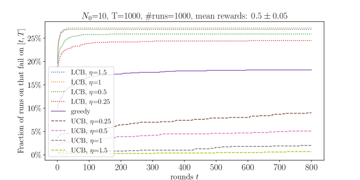
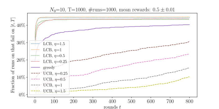
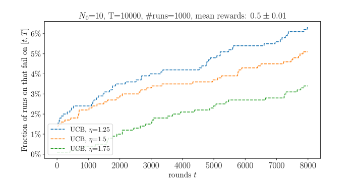
Figure 1: Fail-curves

9 Conclusions and open questions

We examine the dynamics of social learning in a multi-armed bandit scenario, where agents sequentially choose arms and receive rewards, and observe the full history of previous agents. For a range of agents’ myopic behavior, we investigate how they impact exploration, and provide tight upper and lower bounds on the learning failure probabilities and regret rates. As a by-product, we obtain the first general results on the failure of the greedy algorithm in bandits.

With our results as a “departure point”, one could study $\mathtt{BSL}$ in more complex bandit models with many arms and some known structure of rewards. In particular, the greedy algorithm fails for some structures (e.g., our current model) and works well for some others (e.g., when all arms have the same rewards), and it is not at all clear what structures would cause failures and/or be amenable to analysis. Our negative results in Section 7.2 make progress in this direction, as they handle (essentially) arbitrary “Bayesian” structures. However, these guarantees are restricted to the “fully Bayesian” setting when the mean rewards are drawn according to the agents’ prior, and may be weak or vacuous for some correlated priors because of the minimum/infimum in Corollary 7.9.

Appendix A Probability tools

A.1 Proof of Lemma 3.13

Proof.

We use the following sharp lower bound on the tail probability of binomial distribution.

Theorem A.1 (Theorem 9 in Zhang and Zhou (2020)).

Let $n\in\mathbb{N}$ be a positive integer and let $(X_{i})_{i\in[n]}$ be a sequance of i.i.d Bernoulli random variables with prameter $p$. For any $\beta>1$ there exists constants $c_{\beta}$ and $C_{\beta}$ that only rely on $\beta$, such that for all $x$ satisfying $x\in[0,\frac{np}{\beta}]$ and $x+n(1-p)\geq 1$, we have

$${\mathrm{Pr}\left[\,\sum_{i=1}^{n}X_{i}\leq np-x\,\right]}\geq c_{\beta}e^{-C_{\beta}nD(p-\frac{x}{n}||p)},$$

where $D(x||y)$ denotes the KL divergence between two Bernoulli random variables with parameters $x$ and $y$.

We use the above result with $x=n(p-q)$ and $\beta=\frac{1-c}{1-\frac{9}{8}c}$. Note that $\beta>1$ since $c<\frac{1}{2}$. We first verify that $x,\beta$ satisfy the conditions of the lemma. The $x+n(1-p)\geq 1$ condition holds by the assumption $n\geq 1/c$:

$$x+n(1-p)\geq n(1-p)\geq nc\geq 1.$$

As for the $x\leq\frac{np}{\beta}$ condition, by definition of $x$,

$$\frac{np}{x}=\frac{np}{n(p-q)} =\frac{p}{p-q}.$$

Since $p\leq 1-c$ and $\frac{p}{p-q}$ is decreasing in $p$ for $p\geq q$, we can further bound this with

$$\frac{p}{p-q}\geq\frac{1-c}{1-c-q}\geq\frac{1-c}{1-c-\frac{c}{8}}=\beta,$$

where the second inequality follows from $q\geq c/8$ and $q<p\leq 1-c$, together with the fact that $\frac{1-c}{1-c-q}$ is decreasing in $q$ for $q<1-c$. We obtain $x\leq\frac{np}{\beta}$ by rearranging.

Invoking Theorem A.1 with the given values, we obtain

$${\mathrm{Pr}\left[\,\frac{\sum_{i=1}^{n}X_{i}}{n}\leq q\,\right]}\geq c_{\beta}e^{-C_{\beta}nD(q||p)}=\Omega(e^{-O(nD(q||p))}).$$ (A.1)

Next, we use the following type of reverse Pinsker’s inqeuality to upper bound $D(q||p)$.

Theorem A.2 (Götze et al. (2019)).

For any two probability measures $P$ and $Q$ on a finite support $X$, if $Q$ is absolutely continuous with respect to $P$, then the their KL divergence $D(Q||P)$ is upper bounded by $\frac{2}{\alpha_{P}}\delta(Q,P)^{2}$ where $\alpha_{P}=\min_{x\in X}P(x)$ and $\delta(Q,P)$ denotes the total variation distance between $P$ and $Q$.

Setting $P={\text{Bernoulli}}(p)$ and $Q={\text{Bernoulli}}(q)$, we have $\alpha_{P}=\min(p,1-p)$, and $\delta(Q,P)=p-q$ Therefore, since $\min(p,1-p)\geq c$ by assumption, we conclude $D(q||p)\leq O((p-q)^{2}).$ Plugging this back in Equation (A.1) finshes the proof. ∎

A.2 Proof of Lemma 3.14

Our proof will rely on the following doob-style inequality for (super)martingales.

Lemma A.3 (Ville’s Inequality Ville (1939)).

Let $(Z_{n})_{n\geq 0}$ be a positive supermartingale with respect to filtration $(\mathcal{F}_{n})_{n\geq 0}$, i.e. $Z_{n}\geq{\mathbb{E}\left[\,Z_{n+1}|\mathcal{F}_{n}\,\right]}$ for any $n\geq 0$. Then the following holds for any $x>0$,

$${\mathrm{Pr}\left[\,\max_{n\geq 0}Z_{n}\geq x\,\right]}\leq{\mathbb{E}\left[\,Z_{0}\,\right]}/x.$$

In order to use this result, we will define the martingale $Z_{n}:=u^{\sum_{i=1}^{n}(X_{i+1}-q)}$ for a suitable choice of $u$ as specified by the following lemma.

Lemma A.4.

Let $c$ be an absolute constant. For any $p\in(c,1-c)$ and $q\in(0,p)$, there exists a value of $u\in(0,1)$ such that

$$(p\cdot u^{1-q}+(1-p)\cdot u^{-q})=1.$$ (A.2)

In addition, $u$ satisfies

$$p(1-u^{1-q})\geq\Omega(p-q).$$ (A.3)

Proof.

To see why such a $u$ exists, define $f(x)=(p\cdot x^{1-q}+(1-p)\cdot x^{-q})$. It is clear that $f(1)=1$ and $\lim_{x\to 0}f(x)=\infty$ as $\lim_{x\to 0}(1-p)x^{-q}=\infty$. Furthermore,

$$f^{\prime}(x)=p\cdot(1-q)\cdot x^{-q}+(1-p)\cdot(-q)\cdot x^{-q-1},$$

which implies

$$f^{\prime}(1)=p(1-q)-(1-p)q=p-q>0.$$

Therefore, $f(x)$ is decreasing at $x=1$. Since $\lim_{x\to 0}f(x)>f(1)$, this implies that $f(u)=f(1)$ for some $u\in(0,1)$, proving Equation (A.2).

We now prove Equation (A.3), define $x_{0}$ as $x_{0}=\frac{(1-p)q}{p(1-q)}$. Note that $x_{0}<1$ since $p>q$. We claim that $u\leq x_{0}$. To see why, we first note that $f^{\prime}(x)$ can be rewritten as

$$x^{-q-1}\left(xp(1-q)-(1-p)q\right).$$

It is clear that $f^{\prime}(x_{0})=0$. Since $xp(1-q)-(1-p)q$ is increasing in $x$, this further implies that $f^{\prime}(x)>0$ for $x>x_{0}$. Now, if $u>x_{0}$, then since $f^{\prime}(x)>0$ for $x>x_{0}$, we would conclude that $f(u)<f(1)$, which is not possible since $f(u)=f(1)=1$. Therefore, $u\leq x_{0}$ as claimed.

We now claim that $x_{0}^{1-q}\leq 1-p+q$. This would finish the proof since, together with $u\leq x_{0}$, this would imply

$$p(1-u^{1-q}) \geq p(1-x_{0}^{1-q})\geq p(p-q)=\Omega(p-q),$$

where for the last equation we have used the assumption $p\in(c,1-c)$.

To prove the claim, define $\varepsilon:=p-q$. We need to show that $x_{0}^{1-q}\leq 1-\varepsilon$, or equivalently $\ln(x_{0})\leq\frac{\ln(1-\varepsilon)}{1-q}$. By defintion of $x_{0}$, this is equivalent to

$$\ln\left(\frac{(1-p)(p-\varepsilon)}{(1-p+\varepsilon)p}\right)\leq\frac{1}{1-p+\varepsilon}\ln(1-\varepsilon).$$ (A.4)

Fix $p$ and consider both hand sides as a function of $\varepsilon$. Putting $\varepsilon=0$, both hands side coincide as they both equal 0. To prove Euqation (A.4), it suffices to show that as we increase $\varepsilon$, the left hand side decreases faster than the right hand side. Equivalently, we need to show that the derivative of the LHS with respect to $\varepsilon$ is larger than the derivative of the RHS with respect to $\varepsilon$ for $\varepsilon\leq[0,p]$. Taking the derivative with respect to $\varepsilon$ on LHS, we obtain

$$\frac{d}{d\varepsilon}\left(\ln(1-p)+\ln(p-\varepsilon)-\ln(1-p+\varepsilon)-\ln(p)\right)=-\frac{1}{p-\varepsilon}-\frac{1}{1-p+\varepsilon}.$$

Similarly taking the derivative on RHS we obtain

$$\frac{d}{d\varepsilon}\left(\frac{\ln(1-\varepsilon)}{1-p+\varepsilon}\right)=-\frac{1}{(1-\varepsilon)(1-p+\varepsilon)}-\frac{\ln(1-\varepsilon)}{(1-p+\varepsilon)^{2}}.$$

We therefore need to show that

$$\frac{-1}{1-p+\varepsilon}+\frac{-1}{p-\varepsilon}\leq\frac{-1}{(1-p+\varepsilon)(1-\varepsilon)}+\frac{-\ln(1-\varepsilon)}{(1-p+\varepsilon)^{2}}.$$ (A.5)

We note however that

$$\frac{-1}{1-p+\varepsilon}+\frac{-1}{p-\varepsilon}=\frac{\varepsilon-p-1+p-\varepsilon}{(1-p+\varepsilon)(1-\varepsilon)}=\frac{-1}{(1-p+\varepsilon)(1-\varepsilon)}.$$

Therefore Equation (A.5) is equivalent to

$$\frac{-\ln(1-\varepsilon)}{(1-p+\varepsilon)^{2}}\geq 0,$$

which is true since $\varepsilon\in[0,p]$. This proves the claim $x_{0}^{1-q}\leq 1-\varepsilon$, finishing the proof. ∎

We now prove Lemma 3.14 using Lemma A.3 and A.4.

Proof of Lemma 3.14.

Define the random variable $Y_{i}$ as $Y_{i}=X_{i+1}-q$. Note that $Y_{i}$ takes value $1-q$ with probability $p$ and takes $-q$ with probability $1-p$. Set $u$ to be the value specified in Lemma A.4. For $n\geq 0$, define $Z_{n}:=u^{\sum_{i=1}^{n}Y_{i}}$. We first observe that $Z_{n}$ is a martingale with respect to $Y_{1},\ldots,Y_{n}$ as

$${\mathbb{E}\left[\,Z_{n+1}|Y_{1},\dots Y_{n}\,\right]}={\mathbb{E}\left[\,u^{\sum_{i=1}^{n+1}Y_{i}}|Y_{1},\dots Y_{n}\,\right]} =u^{\sum_{i=1}^{n}Y_{i}}\cdot(p\cdot u^{1-q}+(1-p)\cdot u^{-q})$$

$$=u^{\sum_{i=1}^{n}Y_{i}}=Z_{n}.$$

Since $0<u<1$, this further implies

$${\mathrm{Pr}\left[\,\forall n\geq 0:\sum_{i=1}^{n}Y_{i}\geq q-1\,\right]} =1-{\mathrm{Pr}\left[\,\exists n\geq 0:\sum_{i=1}^{n}Y_{i}<q-1\,\right]}$$

$$=1-{\mathrm{Pr}\left[\,\max_{j\in[n]}\{u^{\sum_{i=1}^{j}Y_{i}}\}\geq u^{q-1}\,\right]}$$

$$\geq 1-\frac{{\mathbb{E}\left[\,Z_{1}\,\right]}}{u^{q-1}}$$

$$=1-u^{1-q},$$

where the first inequality follows from Lemma A.3 and the final equality follows from ${\mathbb{E}\left[\,Z_{1}\,\right]}={\mathbb{E}\left[\,Z_{0}\,\right]}={\mathbb{E}\left[\,u^{0}\,\right]}=1$.

Since $Y_{i}$ is a function of $X_{s+1}$, we independently have $X_{1}=1$ with probability $p$. Therefore, with probability $p(1-u^{1-q})$.

$$X_{i}=1\text{ and }\forall n\geq 1:\sum_{i=2}^{n}(X_{i}-q)\geq q-1,$$

which further implies $\sum_{i=1}^{n}(X_{i}-q)\geq 0$. Therefore,

$${\mathrm{Pr}\left[\,\forall n\geq 1:\frac{\sum_{i=1}^{n}X_{i}}{n}\geq q\,\right]}\geq p(1-u^{1-q}) \geq\Omega(p-q),$$

where the inequality follows from Equation (A.3). ∎

A.3 Union of independent events

The following result/proof is standard and provided for the sake of completeness.

Lemma A.5.

Let $A_{1},\dots,A_{n}$ be independent events, each occurring with probability $\geq p$. The probability that at least one of these events occurs is lower bounded by $\min\left\{\,\frac{1}{2},\frac{np}{2}\,\right\}.$

Proof.

Since the events are independent, the probability of at least one of them occurring is lower bounded by ${\mathrm{Pr}\left[\,\cup_{i=1}^{n}A_{i}\,\right]}=1-(1-p)^{n}\geq 1-e^{-np},$ where we have used the ineqaulity $1+x\leq e^{x}$. If $e^{-np}\leq 1/2$, then the claim follows. Otherwise, we have $np<1$. Using the ineqaulity $e^{-x}\leq 1-x/2$ which is valid for $x\leq 1$, we obtain ${\mathrm{Pr}\left[\,\cup_{i=1}^{n}A_{i}\,\right]}\geq\frac{np}{2}$, finishing the proof. ∎

A.4 Joint density function in Corollary 7.9(c)

Recall that Corollary 7.9(c) requires the existence of the joint density of $\mu^{*}(S)$ and $\mu^{*}({\mathcal{A}}\setminus S)$. While this follows from standard arguments, we provide the proof for completeness.

Lemma A.6.

Let $\mu=(\mu_{1},\dots,\mu_{K})\in[0,1]^{K}$ be a random vector with a joint p.d.f. (probability density function) $f$. Fix subset $S\subseteq[K]$, let $\mu^{*}(S):=\max_{i\in S}\mu_{i}$. Then random variables $X=\mu^{*}(S)$ and $Y=\mu^{*}([K]\setminus S)$ have a joint p.d.f.

Proof.

Fix indices $i\in S$, $j\in[K]\setminus S$. Given a vector $\nu\in\mathbb{R}^{K}$, let $\nu_{-i,-j}\in\mathbb{R}^{K-2}$ denote the vector obtained by removing coordinates $i$ and $j$ from $\nu$. For each $x,y\in[0,1]$, define the set

$$B_{i,j}(x,y):=\left\{\,\nu_{-i,-j}:\nu\in[0,1]^{K},\;\max_{i^{\prime}\in S}\nu_{i^{\prime}}\leq x,\;\max_{j^{\prime}\in[K]\setminus S}\nu_{j^{\prime}}\leq y\,\right\}\subset[0,1]^{K-2}.$$

For shorthand, write $\nu=\left(\,\nu_{-i,-j};\nu_{i},\nu_{j}\,\right)$ and $\mathtt{IJ}:=S\times\left(\,[K]\setminus S\,\right)$ in what follows.

We prove $f_{X,Y}$ defined below is the p.d.f. for $(X,Y)$:

$$f_{X,Y}(x,y):=\sum_{(i,j)\in\mathtt{IJ}}\quad\int_{\nu_{-i,-j}\in B_{i,j}(x,y)}f{\left(\,\nu_{-i,-j};x,y\,\right)}\,\;\mathtt{d}\nu_{-i,-j}.$$

More formally, we need to prove that for any $x^{\prime},y^{\prime}\in[0,1]$,

$${\mathrm{Pr}\left[\,X\leq x^{\prime},Y\leq y^{\prime}\,\right]}=\int_{x\leq x^{\prime}}\int_{y\leq y^{\prime}}f_{X,Y}(x,y)\,\;\mathtt{d}y\,\;\mathtt{d}x.$$ (A.6)

Fix $x^{\prime},y^{\prime}\in[0,1]$. We are interested in the event $A:=\left\{\,X\leq x^{\prime},Y\leq y^{\prime}\,\right\}$. Define event

$$A_{i,j}:=A\cap\left\{\,\mu_{i}=\mu^{*}(S),\mu_{j}=\mu^{*}([K]\setminus S)\,\right\},\quad(i,j)\in\mathtt{IJ}.$$

Note that $A=\cup_{(i,j)\in\mathtt{IJ}}A_{i,j}$. Moreover, the intersection $A_{i,j}\cap A_{i^{\prime},j^{\prime}}$ has zero Borel measure whenever $(i,j)\neq(i^{\prime},j^{\prime})$. It follows that

$${\mathrm{Pr}\left[\,A\,\right]} =\sum_{(i,j)\in\mathtt{IJ}}{\mathrm{Pr}\left[\,A_{i,j}\,\right]}$$

$$=\sum_{(i,j)\in\mathtt{IJ}}\int_{\nu_{i}\leq x^{\prime}}\int_{\nu_{j}\leq y^{\prime}}\int_{\nu_{-i,-j}\in B_{i,j}(\nu_{i},\nu_{j})}f(\nu)\;\mathtt{d}\nu$$

$$=\sum_{(i,j)\in\mathtt{IJ}}\int_{x\leq x^{\prime}}\int_{y\leq y^{\prime}}\int_{\nu_{-i,-j}\in B_{i,j}(x,y)}f(\nu_{-i,-j};x,y)\;\mathtt{d}\nu_{-i,-j}\,\;\mathtt{d}y\,\;\mathtt{d}x$$

$$=\int_{x\leq x^{\prime}}\int_{y\leq y^{\prime}}\left(\,\sum_{(i,j)\in\mathtt{IJ}}\int_{\nu_{-i,-j}\in B_{i,j}(x,y)}f(\nu_{-i,-j};x,y)\;\mathtt{d}\nu_{-i,-j}\,\right)\,\;\mathtt{d}y\,\;\mathtt{d}x.\$$

Eq. (A.6) follows by definition of $f_{X,Y}$, completing the proof. ∎

Appendix B Proof of Lemma 4.7

We assume without loss of generality that $\eta>2$. If $\eta\leq 2$, the Lemma’s statement can be made vacuous using large enough constants in $O$. In addition, for mathematical convenience, we will assume that the tape for each arm is infinite, even though the entries after $T$ will never actually be seen by any of the agents.

For each arm $a$, we first separately consider each interval of the form $[n,2n]$ and bound the probability that $\mathtt{UCB}^{\mathtt{tape},\,\eta}_{a,i}$ deviates too much from $\mu_{a}$ for $i\in[n,2n]$. While this can be done crudely by applying a union bound over all $i$, we use the following maximal inequality.

Lemma B.1 (Eq. (2.17) in Hoeffding (1963)).

Given a sequence of i.i.d. random variables $(X_{i})_{i\in[n]}$ in $[0,1]$ such that ${\mathbb{E}\left[\,X_{i}\,\right]}=\mu$, the inequality states that for any $x>0$,

$${\mathrm{Pr}\left[\,\exists i\in[n]:\left|\,\sum_{j=1}^{i}\left(\,X_{j}-\mu\,\right)\,\right|>x\,\right]}\leq 2e^{-\frac{2x^{2}}{n}}.$$

Focusing on some interval of the form $[n,2n]$ for $n\in\mathbb{N}$, and applying this inequality to the reward tape of arm $a$, we conclude that

$${\mathrm{Pr}\left[\,\exists i\in[n,2n]:\left|\,\widehat{\mu}^{\mathtt{tape}}_{a,i}-\mu_{a}\,\right|\geq x\,\right]}\leq O(e^{-\Omega(nx^{2})}).$$ (B.1)

Define $f:=\lceil 64\eta/\Delta^{2}\rceil$. We note that $f=\Theta(\eta/\Delta^{2})$ given the assumption $\eta>2$. In order to bound ${\mathrm{Pr}\left[\,\mathtt{Clean}_{2}^{\eta}\,\right]}$, we will apply this inequality to each interval $[n,2n]$ for $n\geq f$, and take a union bound. Formally,

$$1-{\mathrm{Pr}\left[\,\mathtt{Clean}_{2}^{\eta}\,\right]} \leq{\mathrm{Pr}\left[\,\exists i\geq f:\widehat{\mu}^{\mathtt{tape}}_{2,i}>\mu_{2}+\Delta/8\,\right]} \sqrt{\eta/i}\leq\Delta/8 i\geq f$$ (Since for )

$$\leq\sum_{r=0}^{\infty}{\mathrm{Pr}\left[\,\exists i\in[f2^{r},f2^{r+1}]:\widehat{\mu}^{\mathtt{tape}}_{2,i}>\mu_{2}+\Delta/8\,\right]}$$ (Union bound)

$$\leq O\left(\,\sum_{r=0}^{\infty}e^{-\Omega(\eta 2^{r})}\,\right)$$ (By Eq. (B.1))

$$\leq O\left(\,\sum_{r=0}^{\infty}e^{-\Omega(\eta(r+1))}\,\right) 2^{r}\geq r+1 r\in\mathbb{N}$$ (Since for )

$$=O(\frac{1}{e^{\Omega(\eta)}-1})$$ (Sum of geometric series)

$$\leq O(e^{-\Omega(\eta)}) \eta>2$$ (By )

In order to bound ${\mathrm{Pr}\left[\,\mathtt{Clean}_{1}^{\eta}\,\right]}$, we separately handle the intervals $n<f$ and $n\geq f$. For $n\geq f$, repeating the same argument as above for arm 1 implies

$${\mathrm{Pr}\left[\,\exists i\geq f:\widehat{\mu}^{\mathtt{tape}}_{1,i}<\mu_{1}-\Delta/8\,\right]}\leq O(e^{-\Omega(\eta)}).$$

For $n<f$, we use a modified argument that utilizes the extra $\sqrt{\eta/i}$ term in $\mathtt{UCB}^{\mathtt{tape},\,\eta}_{1,i}$. Instead of bounding the probability $\widehat{\mu}^{\mathtt{tape}}_{1,i}$ having deviation $\Delta/8$, we bound the probability that it deviates by $\sqrt{\eta/i}$. This results in a marked improvement because $\sqrt{\eta/i}$ increases as we decrease $i$. Formally,

$${\mathrm{Pr}\left[\,\exists i\in[1,f]:\widehat{\mu}^{\mathtt{tape}}_{1,i}<\mu_{1}-\sqrt{\eta/i}\,\right]}$$

$$\leq\sum_{r=0}^{\lceil\log(f)\rceil}{\mathrm{Pr}\left[\,\exists i\in[2^{r},2^{r+1}]:\widehat{\mu}^{\mathtt{tape}}_{1,i}<\mu_{1}-\sqrt{\eta/i}\,\right]}$$ (Union bound)

$$\leq\sum_{r=0}^{\lceil\log(f)\rceil}{\mathrm{Pr}\left[\,\exists i\in[2^{r},2^{r+1}]:\widehat{\mu}^{\mathtt{tape}}_{1,i}<\mu_{1}-\sqrt{\eta/2^{r+1}}\,\right]} i$$ (By assumption on )

$$\leq O\left(\,\sum_{r=0}^{\lceil\log(f)\rceil}e^{-\Omega(\eta)}\,\right)$$ (By Eq. (B.1))

$$=O(\lceil\log(f)\rceil e^{-\Omega(\eta)}).$$

Finally, we note that since $\eta>2$,

$$\lceil\log(f)\rceil\leq O(1+\log(f))=O(1+\log(\eta)+\log(1/\Delta)).$$

This implies Eq. (4.4) because $O(\log(\eta)e^{-\Omega(\eta)})$ can be rewritten as $O(e^{-\Omega(\eta)})$ by changing the constant behind $\Omega$.

Appendix C Proof of Theorem 5.1

In this section, we prove Theorem 5.1. We first briefly review some properties of the beta distribution. Throughout the section, we consider a beta distribution with parameters $\alpha,\beta$.

Lemma C.1 (Fact 1 in Agrawal and Goyal (2012b)).

Let $F^{B}_{n,p}$ denote the CDF of the binomial distribution with paramters $n,p$ and $F^{beta}_{\alpha,\beta}$ denote the CDF of the beta distribution. Then,

$$F^{beta}_{\alpha,\beta}(y)=1-F^{B}_{\alpha+\beta-1,y}(\alpha-1)$$

for $\alpha,\beta$ that are positive integers.

Using Hoeffding’s inequality for concentration of the binomial distribution, we immediately obtain the following corollary.

Corollary C.2.

Define $\rho_{\alpha,\beta}:=\frac{\alpha-1}{\alpha+\beta-1}.$ If $X$ is sampled from the beta distribution with parameters $(\alpha,\beta)$,

$${\mathrm{Pr}\left[\,\left|\,X-\rho_{\alpha,\beta}\,\right|\leq y\,\right]}\leq 2e^{-(\alpha+\beta-1)y^{2}}.$$

In addition, letting $Q(.)$ denote the quantile function of the distribution,

$$[Q(\zeta),Q(1-\zeta)]\subseteq\left[\,\rho_{\alpha,\beta}-\sqrt{\frac{\ln(2/\zeta)}{\alpha+\beta-1}},\rho_{\alpha,\beta}+\sqrt{\frac{\ln(2/\zeta)}{\alpha+\beta-1}}\,\right],$$

Let $\alpha_{a,n},\beta_{a,n}$ denote the posterior distribution after observing $n$ entries of the tape for arm $a$. Note that since we are assuming independent priors, the posterior for each arm is independent of the seen rewards of the other arm. Define $M_{a,n}:=\alpha_{a,n}+\beta_{a,n}$. We note that by definition, $\alpha_{a,0},\beta_{a,0}$ coincide with the prior $\alpha_{a},\beta_{a}$. We analogously define $M_{a}:=\alpha_{a}+\beta_{a}$. Define $\rho_{a,n}:=\frac{\alpha_{a,n}-1}{M_{a,n}-1}$ and $\xi_{a,n}:=\frac{\alpha_{a,n}}{M_{a,n}}$. We note that $\xi_{a,n}$ is the mean of the posterior distribution after observing $n$ entries of arm $a$.

Lemma C.3.

For all $n\geq 0$, $\left|\,\widehat{\mu}^{\mathtt{tape}}_{a,n}-\xi_{a,n}\,\right|\leq O\left(\,\frac{M_{a,0}}{n+M_{a,0}}\,\right).$

Proof.

After observing $n$ entries, the posterior parameters satisfy

$$\alpha_{a,n}:=\alpha_{a,0}+\sum_{i\leq n}\mathtt{Tape}_{a,i},\quad\beta_{a,n}:=\beta_{a,0}+\sum_{i\leq n}(1-\mathtt{Tape}_{a,i}).$$

It follows that

$$\xi_{a,n}=\frac{\alpha_{a,0}+\sum_{i\leq n}\mathtt{Tape}_{a,i}}{\alpha_{a,0}+\beta_{a,0}+n}.$$

Defining $X:=\sum_{i\leq n}\mathtt{Tape}_{a,i}$, we can bound the difference between $\xi_{a,n}$ and $\widehat{\mu}^{\mathtt{tape}}_{a,n}$ as

$$\left|\,\frac{\alpha_{a,0}+X}{M_{a,0}+n}-\frac{X}{n}\,\right| =\left|\,\frac{n\alpha_{a,0}+nX-nX-XM_{a,0}}{n(n+M_{a,0})}\,\right|$$

$$=\left|\,\frac{n\alpha_{a,0}-XM_{a,0}}{n(n+M_{a,0})}\,\right|$$

$$\leq\frac{\alpha_{a,0}}{n+M_{a,0}}+\frac{M_{a,0}}{n+M_{a,0}} X\leq n$$ (Since )

$$\leq O\left(\,\frac{M_{a,0}}{n+M_{a,0}}\,\right)$$

∎

Lemma C.4.

For all $n\geq 0$, $\left|\,\xi_{a,n}-\rho_{a,n}\,\right|\leq O\left(\,\frac{1}{n+M_{a,0}}\,\right).$

Proof.

$$\left|\,\frac{\alpha_{a,n}-1}{M_{a,n}-1}-\frac{\alpha_{a,n}}{M_{a,n}}\,\right| =\left|\,\frac{-M_{a,n}+\alpha_{a,n}}{M_{a,n}(M_{a,n}-1)}\,\right|$$

$$\leq\frac{M_{a,n}}{M_{a,n}(M_{a,n}-1)}$$

$$=\frac{1}{M_{a,n}-1}$$

$$=O\left(\,\frac{1}{n+M_{a,0}}\,\right) M_{a,n}=M_{a,0}+n M_{a,0}\geq 1$$ (Since and )

∎

We can now prove Theorem 5.1.

Proof of Theorem 5.1.

We start with part (a). Set $\eta$ to be large enough such that

$$\left|\,\widehat{\mu}^{\mathtt{tape}}_{a,n}-\xi_{a,n}\,\right|\leq\sqrt{\frac{\eta}{n}}.$$

Since $\frac{M_{a}}{n+M_{a}}\leq\frac{M_{a}}{n},$ by Lemma C.3, this can be achieved with $\eta\geq O(M_{a}/\sqrt{N_{0}})$, which proves part (a).

For part (b), set $\eta$ to be large enough such that $\left|\,\widehat{\mu}^{\mathtt{tape}}_{a,n}-\rho_{a,n}\,\right|\leq\frac{1}{2}\cdot\sqrt{\frac{\eta}{n}}.$ Given, Lemmas C.3 and C.4, this can be achieved with $\eta\geq O(M_{a}/\sqrt{N_{0}})$. Since $M-1\geq n$, we can further gaurantee $\frac{\ln(2/\zeta)}{M-1}\leq\frac{\eta}{4n}$ by setting $\eta\geq O(\ln(1/\zeta))$, which finishes the proof together with Corollary C.2. ∎

References

- Acemoglu et al. (2022) Daron Acemoglu, Ali Makhdoumi, Azarakhsh Malekian, and Asuman Ozdaglar. Learning From Reviews: The Selection Effect and the Speed of Learning. Econometrica, 2022. Working paper available since 2017.
- Agrawal and Goyal (2012a) Shipra Agrawal and Navin Goyal. Analysis of Thompson Sampling for the multi-armed bandit problem. In 25nd Conf. on Learning Theory (COLT), 2012a.
- Agrawal and Goyal (2012b) Shipra Agrawal and Navin Goyal. Analysis of thompson sampling for the multi-armed bandit problem. In Conference on learning theory, pages 39–1. JMLR Workshop and Conference Proceedings, 2012b.
- Agrawal and Goyal (2017) Shipra Agrawal and Navin Goyal. Near-optimal regret bounds for thompson sampling. J. of the ACM, 64(5):30:1–30:24, 2017. Preliminary version in AISTATS 2013.
- Audibert and Bubeck (2010) J.Y. Audibert and S. Bubeck. Regret Bounds and Minimax Policies under Partial Monitoring. J. of Machine Learning Research (JMLR), 11:2785–2836, 2010. Preliminary version in COLT 2009.
- Auer et al. (2002a) Peter Auer, Nicolò Cesa-Bianchi, and Paul Fischer. Finite-time analysis of the multiarmed bandit problem. Machine Learning, 47(2-3):235–256, 2002a.
- Auer et al. (2002b) Peter Auer, Nicolò Cesa-Bianchi, Yoav Freund, and Robert E. Schapire. The nonstochastic multiarmed bandit problem. SIAM J. Comput., 32(1):48–77, 2002b. Preliminary version in 36th IEEE FOCS, 1995.
- Bala and Goyal (1998) Venkatesh Bala and Sanjeev Goyal. Learning from neighbours. Review of Economic Studies, 65(3):595–621, 1998.
- Banerjee (1992) Abhijit V. Banerjee. A simple model of herd behavior. Quarterly Journal of Economics, 107:797–817, 1992.
- Barberis and Thaler (2003) Nicholas Barberis and Richard Thaler. A survey of behavioral finance. In Handbook of the Economics of Finance, volume 1, pages 1053–1128. Elsevier, 2003.
- Bastani et al. (2021) Hamsa Bastani, Mohsen Bayati, and Khashayar Khosravi. Mostly exploration-free algorithms for contextual bandits. Management Science, 67(3):1329–1349, 2021. Working paper available on arxiv.org since 2017.
- Bateson (2016) Melissa Bateson. Optimistic and pessimistic biases: a primer for behavioural ecologists. Current Opinion in Behavioral Sciences, 12:115–121, 2016.
- Bayati et al. (2020) Mohsen Bayati, Nima Hamidi, Ramesh Johari, and Khashayar Khosravi. Unreasonable effectiveness of greedy algorithms in multi-armed bandit with many arms. In 33rd Advances in Neural Information Processing Systems (NeurIPS), 2020.
- Bergemann and Välimäki (2006) Dirk Bergemann and Juuso Välimäki. Bandit Problems. In Steven Durlauf and Larry Blume, editors, The New Palgrave Dictionary of Economics, 2nd ed. Macmillan Press, 2006.
- Bikhchandani et al. (1992) Sushil Bikhchandani, David Hirshleifer, and Ivo Welch. A Theory of Fads, Fashion, Custom, and Cultural Change as Informational Cascades. Journal of Political Economy, 100(5):992–1026, 1992.
- Bohren and Hauser (2021) Aislinn Bohren and Daniel N. Hauser. Learning with Heterogeneous Misspecified Models: Characterization and Robustness. Econometrica, 89(6):3025–3077, Nov 2021.
- Bolton and Harris (1999) Patrick Bolton and Christopher Harris. Strategic Experimentation. Econometrica, 67(2):349–374, 1999.
- Bubeck and Cesa-Bianchi (2012) Sébastien Bubeck and Nicolo Cesa-Bianchi. Regret Analysis of Stochastic and Nonstochastic Multi-armed Bandit Problems. Foundations and Trends in Machine Learning, 5(1):1–122, 2012. Published with Now Publishers (Boston, MA, USA). Also available at https://arxiv.org/abs/1204.5721.
- Chang (2000) Edward C Chang, editor. Optimism and pessimism: Implications for theory, research, and practice. American Psychological Association, 2000. See https://www.apa.org/pubs/books/431754A for the table of contents.
- Che and Hörner (2018) Yeon-Koo Che and Johannes Hörner. Recommender systems as mechanisms for social learning. Quarterly Journal of Economics, 133(2):871–925, 2018. Working paper since 2013, titled ’Optimal design for social learning’.
- Chen et al. (2018) Bangrui Chen, Peter I. Frazier, and David Kempe. Incentivizing exploration by heterogeneous users. In Conf. on Learning Theory (COLT), pages 798–818, 2018.
- DeGroot (1974) Morris H. DeGroot. Reaching a Consensus. Journal of the American Statistical Association, 69(345):118–121, 1974.
- den Boer and Zwart (2014) Arnoud V. den Boer and Bert Zwart. Simultaneously learning and optimizing using controlled variance pricing. Management Science, 60(3):770–783, 2014.
- Even-Dar et al. (2006) Eyal Even-Dar, Shie Mannor, and Yishay Mansour. Action elimination and stopping conditions for the multi-armed bandit and reinforcement learning problems. J. of Machine Learning Research (JMLR), 7:1079–1105, 2006.
- Frazier et al. (2014) Peter Frazier, David Kempe, Jon M. Kleinberg, and Robert Kleinberg. Incentivizing exploration. In ACM Conf. on Economics and Computation (ACM-EC), pages 5–22, 2014.
- Fudenberg and Levine (2014) Drew Fudenberg and David K. Levine. Learning with recency bias. Proceedings of the National Academy of Sciences, 111:10826–10829, 2014.
- Fudenberg et al. (2021) Drew Fudenberg, Giacomo Lanzani, and Philipp Strack. Limit Points of Endogenous Misspecified Learning. Econometrica, 89(3):1065–1098, May 2021.
- Gilboa and Schmeidler (1995) Itzhak Gilboa and David Schmeidler. Case-Based Decision Theory. The Quarterly Journal of Economics, 110(3):605–639, 08 1995.
- Gittins et al. (2011) John Gittins, Kevin Glazebrook, and Richard Weber. Multi-Armed Bandit Allocation Indices. John Wiley & Sons, Hoboken, NJ, USA, 2nd edition, 2011.
- Golub and Sadler (2016) Benjamin Golub and Evan D. Sadler. Learning in social networks. In Yann Bramoullé, Andrea Galeotti, and Brian Rogers, editors, The Oxford Handbook of the Economics of Networks. Oxford University Press, 2016.
- Götze et al. (2019) Friedrich Götze, Holger Sambale, and Arthur Sinulis. Higher order concentration for functions of weakly dependent random variables. Electronic Journal of Probability, 24:1–19, 2019.
- Han et al. (2015) Li Han, David Kempe, and Ruixin Qiang. Incentivizing exploration with heterogeneous value of money. In 11th Intl. Conf. on Web and Internet Economics (WINE), pages 370–383, 2015.
- Harrison et al. (2012) J. Michael Harrison, N. Bora Keskin, and Assaf Zeevi. Bayesian dynamic pricing policies: Learning and earning under a binary prior distribution. Management Science, 58(3):570–586, 2012.
- Heidhues et al. (2018) Paul Heidhues, Botond Koszegi, and Philipp Strack. Unrealistic expectations and misguided learning. Econometrica, 86(4):1159–1214, 2018.
- Hoeffding (1963) Wassily Hoeffding. Probability inequalities for sums of bounded random variables. Journal of the American statistical association, 58(301):13–30, 1963.
- Hörner and Skrzypacz (2017) Johannes Hörner and Andrzej Skrzypacz. Learning, experimentation, and information design. In Bo Honoré, Ariel Pakes, Monika Piazzesi, and Larry Samuelson, editors, Advances in Economics and Econometrics: 11th World Congress, volume 1, page 63–98. Cambridge University Press, 2017.
- Immorlica et al. (2020) Nicole Immorlica, Jieming Mao, Aleksandrs Slivkins, and Steven Wu. Incentivizing exploration with selective data disclosure. In ACM Conf. on Economics and Computation (ACM-EC), pages 647–648, 2020. Working paper available at https://arxiv.org/abs/1811.06026.
- Jedor et al. (2021) Matthieu Jedor, Jonathan Louëdec, and Vianney Perchet. Be greedy in multi-armed bandits, 2021. Working paper, available on https://arxiv.org/abs/2101.01086.
- Kahneman and Tversky (1982) Daniel Kahneman and Amos Tversky. Judgment under uncertainty: Heuristics and biases. Cambridge University Press, 1982.
- Kannan et al. (2018) Sampath Kannan, Jamie Morgenstern, Aaron Roth, Bo Waggoner, and Zhiwei Steven Wu. A smoothed analysis of the greedy algorithm for the linear contextual bandit problem. In Advances in Neural Information Processing Systems (NIPS), pages 2231–2241, 2018.
- Kaufmann et al. (2012) Emilie Kaufmann, Nathaniel Korda, and Rémi Munos. Thompson sampling: An asymptotically optimal finite-time analysis. In 23rd Intl. Conf. on Algorithmic Learning Theory (ALT), pages 199–213, 2012.
- Keller et al. (2005) Godfrey Keller, Sven Rady, and Martin Cripps. Strategic Experimentation with Exponential Bandits. Econometrica, 73(1):39–68, 2005.
- Keskin and Zeevi (2018) N. Bora Keskin and Assaf Zeevi. On incomplete learning and certainty-equivalence control. Oper. Res., 66(4):1136–1167, 2018.
- Kremer et al. (2014) Ilan Kremer, Yishay Mansour, and Motty Perry. Implementing the “wisdom of the crowd”. J. of Political Economy, 122(5):988–1012, 2014. Preliminary version in ACM EC 2013.
- Lai and Robbins (1982) T.L. Lai and Herbert Robbins. Iterated least squares in multiperiod control. Advances in Applied Mathematics, 3(1):50–73, 1982.
- Lai and Robbins (1985) Tze Leung Lai and Herbert Robbins. Asymptotically efficient Adaptive Allocation Rules. Advances in Applied Mathematics, 6:4–22, 1985.
- Lanzani (2023) Giacomo Lanzani. Dynamic Concern for Misspecification, 2023. Working paper.
- Lattimore and Szepesvári (2020) Tor Lattimore and Csaba Szepesvári. Bandit Algorithms. Cambridge University Press, Cambridge, UK, 2020.
- Lazer and Friedman (2007) David Lazer and Allan Friedman. The network structure of exploration and exploitation. Administrative Science Quarterly, 52:667–694, 2007.
- Luce (1959) R. Duncan Luce. Individual Choice Behavior: A Theoretical Analysis. Wiley, New York, NY, USA, 1959.
- Mansour et al. (2020) Yishay Mansour, Aleksandrs Slivkins, and Vasilis Syrgkanis. Bayesian incentive-compatible bandit exploration. Operations Research, 68(4):1132–1161, 2020. Preliminary version in ACM EC 2015.
- Myers (1976) Jerome L. Myers. Probability learning and sequence learning. In W.K. Estes, editor, Handbook of Learning and Cognitive Processes: Approaches to Human Learning and Motivation, pages 171–205. Erlbaum, Hillsdale, NJ, 1976.
- Puri and Robinson (2007) Manju Puri and David T. Robinson. Optimism and economic choice. Journal of Financial Economics, 86(1):71–99, 2007.
- Raghavan et al. (2023) Manish Raghavan, Aleksandrs Slivkins, Jennifer Wortman Vaughan, and Zhiwei Steven Wu. Greedy algorithm almost dominates in smoothed contextual bandits. SIAM J. on Computing (SICOMP), 52(2):487–524, 2023. Preliminary version at COLT 2018. Working paper available at arxiv.org/abs/2005.10624.
- Russo et al. (2018) Daniel Russo, Benjamin Van Roy, Abbas Kazerouni, Ian Osband, and Zheng Wen. A tutorial on thompson sampling. Foundations and Trends in Machine Learning, 11(1):1–96, 2018. Published with Now Publishers (Boston, MA, USA). Also available at https://arxiv.org/abs/1707.02038.
- Sellke and Slivkins (2022) Mark Sellke and Aleksandrs Slivkins. The price of incentivizing exploration: A characterization via thompson sampling and sample complexity. Operations Research, 71(5), 2022. Preliminary version in ACM EC 2021.
- Slivkins (2019) Aleksandrs Slivkins. Introduction to multi-armed bandits. Foundations and Trends in Machine Learning, 12(1-2):1–286, November 2019. Published with Now Publishers (Boston, MA, USA). Also available at https://arxiv.org/abs/1904.07272. Latest online revision: Jan 2022.
- Slivkins (2023) Aleksandrs Slivkins. Exploration and persuasion. In Federico Echenique, Nicole Immorlica, and Vijay Vazirani, editors, Online and Matching-Based Market Design. Cambridge University Press, 2023. Also available at http://slivkins.com/work/ExplPers.pdf.
- Smith and Sørensen (2000) Lones Smith and Peter Sørensen. Pathological outcomes of observational learning. Econometrica, 68:371–398, 2000.
- Thompson (1933) William R. Thompson. On the likelihood that one unknown probability exceeds another in view of the evidence of two samples. Biometrika, 25(3-4):285–294, 1933.
- Ville (1939) Jean Ville. Etude critique de la notion de collectif. Bull. Amer. Math. Soc, 45(11):824, 1939.
- Vulkan (2000) Nir Vulkan. An economist’s perspective on probability matching. Journal of Economic Surveys, 14:101–118, 2000.
- Welch (1992) Ivo Welch. Sequential sales, learning, and cascades. The Journal of finance, 47:695–732, 1992.
- Zhang and Zhou (2020) Anru R Zhang and Yuchen Zhou. On the non-asymptotic and sharp lower tail bounds of random variables. Stat, 9(1):e314, 2020.