Microwave electrometry with multi-photon coherence in Rydberg atoms

Abstract

A scheme for measurement of microwave (MW) electric field is proposed via multi-photon coherence in Rydberg atoms. It is based on the three-photon electromagnetically induced absorption (TPEIA) spectrum. In this process, the multi-photon produces a narrow absorption peak, which has a larger magnitude than the electromagnetically induced transparency (EIT) peak under the same conditions. The TPEIA peak is sensitive to MW fields, and can be used to measure MW electric field strength. It is interesting to find that the magnitude of TPEIA peaks shows a linear relationship with the MW field strength. The simulation results show that the minimum detectable strength of the MW fields is about 1/10 that based on an common EIT effect, and the probe sensitivity is improved by about 4 times. Furthermore, the MW sensing based on three-photon coherence shows a broad tunability, and the scheme may be useful for designing novel MW sensing devices.

I Introduction

Atom-based metrology has been widely used in many fields, such as atomic clocks, measurement of temperature, frequency, magnetic and electric fields, due to the unique properties of atoms and molecules [38, 41, 39, 40, 4]. Recently, Rydberg-atom-based microwave electrometry arises great interest [37, 36, 4]. Rydberg atoms with one or more electrons of large principal quantum numbers are sensitive to electric fields, and can coherently interact with a microwave (MW) electric field. It can significantly increase the accuracy and repeatability of measurement. The main research works are based on electromagnetically induced transparency (EIT) and Aulter-Towns splitting [1, 2, 3], where two laser fields drove atoms to their Rydberg states and Rydberg EIT splitting induced by a MW field was used for MW electrometry [4, 5, 6, 7, 8]. New achievements about MW measurement include Rydberg-atom-based superheterodyne receiver [9], enhanced MW metrology by population repumping [10], broadband terahertz wave detection [44], arrival angle of microwave signals [45, 43], continuous measurement [11] and auxiliary transition [12], and radio-frequency phase measurement [13, 14], etc.

It is know that an EIT system has good coherence and its probe spectrum is widely used for MW measurement. Recently, three-photon coherence attracts researchers’ interest. For example, observation of three-photon electromagnetically induced absorption (TPEIA) [17] in atomic systems, constructive interference in the three-photon absorption [15, 16], demonstration of three-photon coherence condition [18], and its extention to Rydberg atoms [19]. Three-photon coherence has important applications, such as overcoming residual Doppler shifts [20], miniaturizing of MW field sensors and receivers [21] and its dependence on the AT splitting with two coupling lasers [22]. While, few reaserch involves MW measurement based on three-photon coherence.

In this paper, we propose a scheme to measure MW electric fields based on three-photon coherence in Rydberg atoms. A probe and a control fields counter-propagate through the atomic system [23]. The ${}^{87}{\rm{Rb}}$ atoms are excited from the ground states to the Rydberg states, and the absorption spectrum of three-photon transition shows a single absorption peak around the resonant frequency. Due to three-photon coherence, a strong TPEIA peak appears under the three-photon resonance condition. It is interesting to find that the TPEIA peak changes linearly with the MW electric field strength. This may be used to detect the MW electric field. The simulation results show the sensitivity is enhanced by about 4 times and its minimum detectable strength of the MW electric field can be increased by more than one order of magnitude, compared with a common EIT scheme. Also, the scheme shows a wide tunability. This may help to design novel MW sensing devices.

(a)

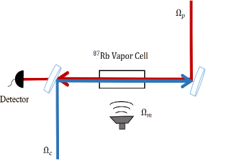
(b)

Figure 1: (a) Four-level Rydberg atom model and (b) schematic diagram of experimental setup including an atoms cell, probe (${\Omega_{p}}$), coupling (${\Omega_{c}}$), a microwave signal generator and detector.

II MODEL AND BASIC EQUATION

Fig. 1(a) shows a four-level ladder-type atomic system. The relevant atomic energy levels of ${}^{87}{\rm{Rb}}$ are $5{S_{1/2}}$ ($|1\rangle$) , $5{P_{3/2}}$ ($|2\rangle$), $53{D_{5/2}}$ ($|3\rangle$), and $54{P_{3/2}}$ ($|4\rangle$). A probe laser ${\Omega_{p}}$ with a wavelength of ${\lambda_{p}}\sim 780$ nm and a coupling laser ${\Omega_{c}}$with ${\lambda_{c}}\sim 480$ nm counter-propagate through the atoms and drive $|1\rangle\leftrightarrow|2\rangle$ and $|2\rangle\leftrightarrow|3\rangle$ transition, respectively. A MW field drives the Rydberg transition of the states $|3\rangle$ to $|4\rangle$. A similar system has been used in intracavity EIT [26], THz field measurement [27], nonlinear optical effects [28], and so on.

In the interaction picture and after the rotating wave approximation, the Hamiltonian of the system can be written as

$$\begin{array}[]{*{20}{l}}H&=-\hbar[{\Delta_{p}}|2\rangle\langle 2|+\left({{\Delta_{p}}+{\Delta_{c}}}\right)|3\rangle\langle 3|\\ &\quad+\left({{\Delta_{p}}+{\Delta_{c}}-{\Delta_{m}}}\right)|4\rangle\langle 4|+{\Omega_{p}}|1\rangle\langle 2|\\ &\quad+{\Omega_{c}}|2\rangle\langle 3|+{\Omega_{m}}|3\rangle\langle 4|+{\rm{H}}.{\rm{C}}.],\end{array}$$ (1)

where H is the interaction Hamiltonian, the Rabi frequency is ${\Omega_{p}}={\mu_{12}}{E_{p}}/\hbar$, ${\Omega_{c}}={\mu_{23}}{E_{c}}/\hbar$, and ${\Omega_{m}}={\mu_{34}}{E_{m}}/\hbar$. ${\Delta_{p}}={\omega_{p}}-{\omega_{12}}$, ${\Delta_{c}}={\omega_{c}}-{\omega_{23}}$, and ${\Delta_{m}}={\omega_{m}}-{\omega_{34}}$ denote the detunings of the corresponding fields, respectively. ${\mu_{ij}}$ (i, j = 1, 2, 3, 4) is the transition dipole moment from state $|i\rangle$ to state $|j\rangle$. The dynamic evolution of the system can be described using the density-matrix method as follows [30]:

$$\dot{\rho}=-\frac{i}{\hbar}[H,\rho]+L\left(\rho\right),$$ (2)

where ${L\left(\rho\right)}$ denotes the decoherence processes. The time evolution of density matrix elements can be written as

$$\begin{split}&{\dot{\rho}_{11}}={\Gamma_{2}}{\rho_{22}}-i\left({{\rho_{12}}-{\rho_{21}}}\right){\Omega_{p}},\\ &{\dot{\rho}_{22}}=-{\Gamma_{2}}{\rho_{22}}+{\Gamma_{3}}{\rho_{33}}-i[({\rho_{23}}-{\rho_{32}}){\Omega_{c}}+({\rho_{12}}-{\rho_{21}}){\Omega_{p}}],\\ &{\dot{\rho}_{33}}=-{\Gamma_{3}}{\rho_{33}}+{\Gamma_{4}}{\rho_{44}}-i[({\rho_{32}}-{\rho_{23}}){\Omega_{c}}+({\rho_{34}}-{\rho_{43}}){\Omega_{m}}],\\ &{\dot{\rho}_{44}}=-{\Gamma_{4}}{\rho_{44}}-i\left({{\rho_{43}}-{\rho_{34}}}\right){\Omega_{m}},\\ &{\dot{\rho}_{21}}=-\frac{1}{2}{\Gamma_{2}}{\rho_{21}}-i[{\Delta_{p}}{\rho_{21}}-{\rho_{31}}{\Omega_{c}}-({\rho_{11}}+{\rho_{22}}){\Omega_{p}}],\\ &{\dot{\rho}_{31}}=-\frac{1}{2}{\Gamma_{3}}{\rho_{31}}-i[{\Delta_{1}}{\rho_{31}}-{\rho_{21}}{\Omega_{c}}-{\rho_{41}}{\Omega_{m}}+{\rho_{32}}{\Omega_{p}}],\\ &{\dot{\rho}_{41}}=-\frac{1}{2}{\Gamma_{4}}{\rho_{41}}-i({\Delta_{2}}{\rho_{41}}-{\rho_{31}}{\Omega_{m}}+{\rho_{42}}{\Omega_{p}}),\\ &{\dot{\rho}_{32}}=-{\gamma_{32}}{\rho_{32}}-i[{\Delta_{c}}{\rho_{32}}+({\rho_{33}}-{\rho_{22}}){\Omega_{c}}-{\rho_{42}}{\Omega_{m}}+{\rho_{31}}{\Omega_{p}}],\\ &{\dot{\rho}_{42}}=-{\gamma_{42}}{\rho_{42}}-i({\Delta_{3}}{\rho_{42}}+{\rho_{43}}{\Omega_{c}}-{\rho_{32}}{\Omega_{m}}+{\rho_{41}}{\Omega_{p}}),\\ &{\dot{\rho}_{43}}=-{\gamma_{43}}{\rho_{43}}-i[-{\Delta_{m}}{\rho_{43}}+{\rho_{42}}{\Omega_{c}}+({\rho_{44}}-{\rho_{33}}){\Omega_{m}}],\end{split}$$ (3)

with ${\rho_{ij}}{\rm{=}}{\rho^{*}}_{ji}$ and the closure relation $\sum\nolimits_{j}{{\rho_{jj}}}=1$, (i,j=1,2,3,4). Here, ${\Delta_{1}}={\Delta_{p}}+{\Delta_{c}}$, ${\Delta_{2}}={\Delta_{p}}+{\Delta_{c}}-{\Delta_{m}}$, and ${\Delta_{3}}={\Delta_{c}}-{\Delta_{m}}$. ${\gamma_{ij}}$ is the decay from the states $|i\rangle$ to $|j\rangle$, and ${\gamma_{ij}}=({\Gamma_{i}}+{\Gamma_{j}})/2$, ${\Gamma_{i}}$ is the population decay rate. We consider $\rho_{11}^{(0)}=1$, $\rho_{ij}^{(0)}=0$. The coherence term ${\rho_{21}}$ can be obtained by solving the above equation. With consideration of the residual Doppler effect, the frequency detunings of the control and probe fields are modified as ${{\rm{\delta}}_{c}}={\Delta_{c}}-{k_{c}}v$, ${{\rm{\delta}}_{p}}={\Delta_{p}}+{k_{p}}v$, where${k_{c}}=2\pi/{\lambda_{c}}$, ${k_{p}}=2\pi/{\lambda_{p}}$, and the susceptibility of the Rydberg atoms is then Doppler-averaged:

$$\chi{\rm{=}}\frac{{2N{{\left|{{\mu_{12}}}\right|}^{2}}}}{{\hbar{\varepsilon_{0}}{\Omega_{p}}}}\frac{1}{{\sqrt{\pi}u}}\int_{-\infty}^{+\infty}{{\rho_{21}}}{e^{-\frac{{{v^{2}}}}{{{u^{2}}}}}}dv,$$ (4)

where N is Rydberg atom density. ${{\mu_{12}}}$ is the dipole moment of transition $|1\rangle\leftrightarrow|2\rangle$, ${{\varepsilon_{0}}}$ is the dielectric constant of vacuum, $u=\sqrt{2{k_{B}}T/m}$ is the most probable velocity of the atoms, ${{k_{B}}}$ is the Boltzmann constant, T is the temperature of system, m is the mass of the atom. Then, we obtain the three-photon coherence term in ${\rho_{21}}$ [31, 32], and the three-photon coherence part of the atomic susceptibility is

$$\begin{array}[]{*{20}{l}}{\chi_{{\rm{TPC}}}}&{\rm{=}}\frac{{2N{{\left|{{\mu_{12}}}\right|}^{2}}}}{{\hbar{\varepsilon_{0}}{\Omega_{p}}}}\frac{1}{{\sqrt{\pi}u}}\int_{-\infty}^{+\infty}{\frac{{i\Omega_{m}^{2}{\Omega_{c}}}}{{{C_{5}}{C_{6}}}}\frac{1}{{{C_{7}}}}}\\ &\times\frac{{i{\Omega_{m}}[{C_{2}}\Omega_{c}^{2}+{C_{1}}(-{C_{2}}{C_{3}}-\Omega_{m}^{2})]+{C_{1}}^{2}\Omega_{m}^{2}\Omega_{p}^{3}{\Omega_{c}}}}{{{C_{1}}{\Omega_{m}}\Omega_{p}^{2}({C_{2}}-{C_{4}}){C_{8}}+{C_{9}}}}dv,\end{array}$$ (5)

where ${C_{1}}=i{\Delta_{m}}-{G_{34}}$, ${C_{2}}={G_{23}}+i{\delta_{c}}$, ${C_{3}}={G_{24}}+i({\delta_{c}}-{\Delta_{m}})$, ${C_{4}}={\Gamma_{4}}/2+i({\delta_{c}}+{\delta_{p}}-{\Delta_{m}})$, ${C_{5}}={\Gamma_{2}}/2+i{\delta_{p}}$, ${C_{6}}={\Gamma_{3}}/2+i({\delta_{c}}+{\delta_{p}})$, ${C_{7}}{\rm{=}}[(i{C_{1}}{C_{4}}{C_{5}}{C_{6}}-\Omega_{c}^{2}){\Omega_{m}}+i{C_{1}}{C_{5}}{\Omega_{m}}(\Omega_{p}^{2}-\Omega_{m}^{2})]$, ${C_{8}}{\rm{=}}[{C_{1}}({C_{5}}{C_{6}}-\Omega_{c}^{2}){\Omega_{m}}+{C_{1}}{C_{5}}({\Omega_{m}}-{C_{5}}\Omega_{c}^{2})]$, ${C_{9}}{\rm{=}}[i{\Omega_{m}}({C_{2}}\Omega_{c}^{2}-i{C_{1}}{C_{2}}{C_{3}}+{C_{1}}\Omega_{m}^{2})+{C_{1}}\Omega_{p}^{2}]$, ${G_{34}}=({\Gamma_{3}}+{\Gamma_{4}})/2$, and ${G_{24}}=({\Gamma_{2}}+{\Gamma_{4}})/2$.

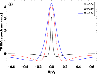
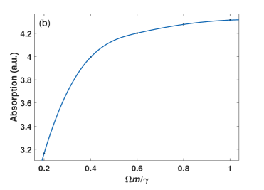
Figure 2: (a) The TPEIA spectrum and (b) peak intensity as a function of the MW field strength, with ${\Omega_{p}}=0.001\gamma$, ${\Omega_{c}}=3{\rm{MHz}}$, ${\Gamma_{3}}{\rm{=}}0.2\gamma$, ${\Gamma_{4}}{\rm{=}}0.01\gamma$. ($\gamma=2\pi\times 1{\rm{MHz}}$).

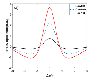
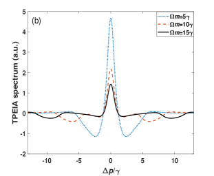
Figure 3: (a) The Doppler-averaged TPEIA spectrum and (b) variation of the TPEIA spectrum with MW field. The other parameters are the same as in Fig. 2(a).

III RESULTS AND DISCUSSION

We first consider the TPEIA spectrum changing with the MW field in a Doppler-free scheme, where the probe field counter-propagates with the control field (see Fig. 2). The ${}^{87}{\rm{Rb}}$ atomic density is $N={10^{-7}}{\rm{c}}{{\rm{m}}^{-3}}$ and spontaneous decay ${\Gamma_{2}}=6\gamma=2\pi\times 6{\rm{MHz}}$ in the following discussion [4]. And the following discussion is scaled by $\gamma$ for simplicity. Fig. 2(a) shows that the TPEIA signal has one absorption peak through the three-photon process when the lasers interact with atoms resonantly. The basic property of TPEIA agree well with the previous study [17, 33], and here we pay attention to the variation of TPEIA with MW fields. For a weak MW field, the TPEIA peak increases with the strength of MW field, as shown in Fig. 2(a), the absorption peak becomes strong with increase of the MW field strength, and the peak linewidth becomes a little broad due to homogenous broadening effect. Thanks to the three-photon coherence, the population transfers from the ground state to the Rydberg state, and the peak value of absorption spectrum can be improved in the range of weak MW field. Fig. 2(b) shows the variations of magnitude of TPEIA peak as a function of the MW field strength. The TPEIA peak becomes strong by increasing MW field, and the linewidth remains narrow. While, the magnitude of TPEIA peak changes nonlinearly with the MW field strength, which may be not suitable for the linear measurement of MW electric field.

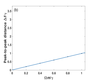
Figure 4: (a) The variations of absorption peak intensity as a function of the MW field strength on the condition of residual Doppler effect and (b) Distance of two transmission peaks ${\Delta_{f}}$ versus the MW field strength. The other parameters are the same as in Fig. 2(a).

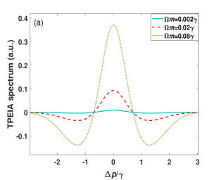
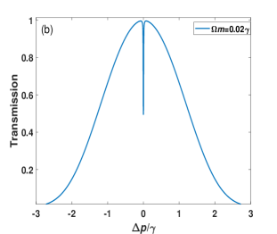
Figure 5: (a) Doppler-averaged TPEIA spectrum and (b) transmission spectrum of EIT. The other parameters are the same as in Fig. 2(a).

Generally, most of the experiments are performed in a room temperature vapour. So, the Doppler effect is obvious due to mismatch of the coupling-field wavelength, where the probe and control fields counter-propagate through the atomic vapor. The variations of the absorption spectrum are shown in Fig. 3(a). The TPEIA peak becomes strong with increase of the MW field. However, when the strength of the MW field is further increases, the TPEIA signal is suppressed and two transmission windows far away from resonance (see Fig. 3(b)). We pay more attention to the enhanced TPEIA peak and explore its application in precise measurement.

It is interesting to find that the magnitude of TPEIA peak varies linearly with the MW field, as shown in Fig. 4(a). The numerical results show that the curve slop based on three-photon coherence is about 4. Fig. 4(b) shows the linear measurement of MW field based on the common EIT method, where the frequency splitting of EIT peaks changes linearly with the MW electric field strength. The slope of measurement curve based on EIT is about 1 from simulation. The comparison of Fig. 4(a) and Fig. 4(b) shows that the curve slope based on TPEIA is about 4 times larger than that of EIT method. The MW electric field strength could be estimated from changes in the magnitude of TPEIA peaks. It is known that, the larger curve slope under the same condition results in the better detection sensitivity. This indicates that the probe sensitivity could be improved by about a factor of 4 due to the three-photon coherence.

It is important to detect the minimum strength of the MW field for precise measurement. Fig. 5(a) shows the minimum detectable strength ${\rm{M}}{{\rm{W}}_{\min}}$ for the three-photon resonance case. According to the Rayleigh criterion [35], the the corresponding spectrum resolution is about 0.02$\gamma$, which means the minimum detectable strength of the MW field is about 0.02$\gamma$ based on the EIT scheme, as shown in Fig. 5(b). Our simulation results show that the minimum detectable strength of the MW field is about 0.002$\gamma$ for the TPEIA spectrum, which is about 1/10 that based on an common EIT effect (see Fig. 5(a)). This indicates that the minimum detectable strength could be improved by 10 times due to the three-photon coherence.

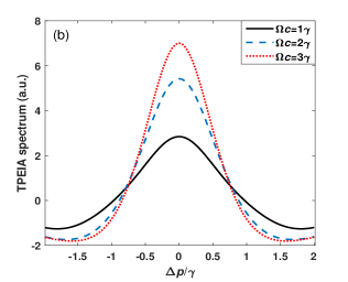
Figure 6: (a) The effect of large MW field on the intensity of the Doppler-averaged TPEIA spectrum and (b) peak intensity as a function of the control field strength with ${\Omega_{m}}=2.8\gamma$. The other parameters are the same as in Fig. 2(a).

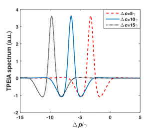
Figure 7: Doppler-averaged TPEIA spectrum for different control field detuning ${\Delta_{c}}$, with ${\Omega_{m}}=\gamma$. The other parameters are the same as in Fig. 2(a).

The above discussions deal with the weak MW field. In the dressed-state picture, the probe and control transition consist of a classical Rydberg EIT scheme. There is an EIT window around the resonant frequency, and it can be understood in the EIT theory [42]. The coupling fields ${\Omega_{c}}$ dresses the states $|2\rangle$ and $|3\rangle$, and two new eigenstates appear, i.e., $|+\rangle$ and $|-\rangle$. With coupling of the probe field, two transition channels appear, $|1\rangle\to|+\rangle$ and $|1\rangle\to|-\rangle$. When the MW field drives the Rydberg transition $|3\rangle\to|4\rangle$, the Rydberg-EIT is disturbed and an enhanced absorption peak builds up, which is referred to be as TPEIA.

Fig. 6(a) shows the effect of the large MW field on the magnitude of the Doppler-averaged TPEIA spectrum. For example, when the MW field strength ${\Omega_{m}}\leq 2.8\gamma$, the TPEIA peak becomes strong with increase of the MW field, as shown Fig. 6(a). While, the TPEIA peak decreases with the further increase of the MW field. So, the TPEIA peak reaches a maximum at ${\Omega_{m}}=2.8\gamma$ under the given condition. This is because the two dressed states induced by the MW field are well separated, and the AT splitting of Rydberg EIT is dominant over TPEIA peak in the regime of the large MW field [19]. The constructive interference for three-photon coherence gradually weakens. When the TPEIA peak decreases with ${\Omega_{m}}$, the peak-to-peak distance of the two transmission peaks increases with ${\Omega_{m}}$, as shown in Fig. 3(a). This effect can be well-understood in the dressed-state picture [34]. The effect of the control field on the intensity of the absorption spectrum is shown in Fig. 6(b). The magnitude of TPEIA peak increases when the control field becomes strong. The strong control field induces the good multi-photon coherence and contributes to the large TPEIA peak. Of course, if the control field is too large, the Rydberg EIT evolves into Aulter-Tonwns splitting, and the inter-path interference weakens, resulting in decrease of TPEIA peak.

In addition, the numerical results show that the linewidth of the absorption spectrum is about 1.15$\gamma$. The linewidth of TPEIA peak is a little broader than that of Doppler-free scheme. This is due to the residual Doppler effect as a result of the temperature of the atomic vapor. The above discussions are based on resonant interaction of the control field. Fig. 7 shows the effect of the control field detuning on the TPEIA spectrum. The figure shows that the absorption window shifts with the control field detuning ${\Delta_{c}}$. While the width and peak value of the TPEIA spectrum basically remain unchanged. This means that the scheme has a broad detection range and some tunability.

IV Conclusion

In summary, we theoretically investigate TPEIA spectrum of Rydberg atoms and propose to use three-photon coherence to detect the weak MW electric field. Due to the multi-photon coherence, there is constructive interference in the TPEIA at the resonant frequency. It is interesting to find that the magnitude of TPEIA peaks change linearly with the MW field, which can be used to detect the MW electric field. The numerical results show the sensitivity based on TPEIA is about 4 times larger than that of the EIT scheme. Its minimum detectable strength is about one order of magnitude smaller than that of the EIT scheme. Moreover, the MW measurement based on TPEIA shows a broad detection range and some tunability. The proposed scheme may help to design novel MW-sensing devices.

References

- [1] T. Gallagher, Rydberg Atoms. Cambridge, U.K.: Cambridge University, 2005.
- [2] K. J. Boller, A. Imamoğlu, and S. E. Harris, “Observation of electromagnetically induced transparency,” Phys. Rev. Lett., vol. 66, no. 20, p. 2593, 1991.
- [3] G. Alzetta, “Induced transparency,” Phys. Today, vol. 50, no. 7, pp. 36–42, 1997.
- [4] J. A. Sedlacek, A. Schwettmann, H. Kübler, R. Löw, T. Pfau, and J. P. Shaffer, “Microwave electrometry with Rydberg atoms in a vapour cell using bright atomic resonances,” Nat. Phys., vol. 8, no. 11, pp. 819–824, 2012.
- [5] H. Cheng, H. Wang, S. Zhang, P. Xin, J. Luo, and H. Liu, “High resolution electromagnetically induced transparency spectroscopy of Rydberg 87 Rb atom in a magnetic field,” Opt. Exp., vol. 25, no. 26, pp. 33 575–33 587, 2017.
- [6] M. T. Simons, J. A. Gordon, C. L. Holloway, D. A. Anderson, S. A. Miller, and G. Raithel, “Using frequency detuning to improve the sensitivity of electric field measurements via electromagnetically induced transparency and Autler-Townes splitting in Rydberg atoms,” Appl. Phys. Lett., vol. 108, no. 17, p. 174101, 2016.
- [7] H. Fan, S. Kumar, J. Sedlacek, H. Kübler, S. Karimkashi, and J. P. Shaffer, “Atom based RF electric field sensing,” J. Phys. B: At. Mol. Opt. Phys., vol. 48, no. 20, p. 202001, 2015.
- [8] J. Sedlacek, A. Schwettmann, H. Kübler, and J. Shaffer, “Atom-based vector microwave electrometry using rubidium Rydberg atoms in a vapor cell,” Phys. Rev. Lett., vol. 111, no. 6, p. 063001, 2013.
- [9] M. Jing, Y. Hu, J. Ma, H. Zhang, L. Zhang, L. Xiao, and S. Jia, “Atomic superheterodyne receiver based on microwave-dressed Rydberg spectroscopy,” Nat. Phys., vol. 16, no. 9, pp. 911–915, 2020.
- [10] N. Prajapati, A. K. Robinson, S. Berweger, M. T. Simons, A. B. Artusio-Glimpse, and C. L. Holloway, “Enhancement of electromagnetically induced transparency based Rydberg-atom electrometry through population repumping,” Appl. Phys. Lett., vol. 119, no. 21, p. 214001, 2021.
- [11] M. T. Simons, A. B. Artusio-Glimpse, C. L. Holloway, E. Imhof, S. R. Jefferts, R. Wyllie, B. C. Sawyer, and T. G. Walker, “Continuous radio-frequency electric-field detection through adjacent Rydberg resonance tuning,” Phys. Rev. A, vol. 104, no. 3, p. 032824, 2021.
- [12] F. D. Jia, X. B. Liu, J. Mei, Y. H. Yu, H. Y. Zhang, Z. Q. Lin, H. Y. Dong, J. Zhang, F. Xie, and Z. P. Zhong, “Span shift and extension of quantum microwave electrometry with Rydberg atoms dressed by an auxiliary microwave field,” Phys. Rev. A, vol. 103, no. 6, p. 063113, 2021.
- [13] M. T. Simons, A. H. Haddab, J. A. Gordon, and C. L. Holloway, “A Rydberg atom-based mixer: Measuring the phase of a radio frequency wave,” Appl. Phys. Lett., vol. 114, no. 11, p. 114101, 2019.
- [14] L. Lin, Y. He, Z. Yin, D. Li, Z. Jia, Y. Zhao, B. Chen, and Y. Peng, “Sensitive detection of radio-frequency field phase with interacting dark states in Rydberg atoms,” Appl. Opt., vol. 61, no. 6, pp. 1427–1433, 2022.
- [15] D. McGloin, D. Fulton, and M. Dunn, “Electromagnetically induced transparency in N-level cascade schemes,” Opt. Commun., vol. 190, no. 1-6, pp. 221–229, 2001.
- [16] C. Carr, M. Tanasittikosol, A. Sargsyan, D. Sarkisyan, C. S. Adams, and K. J. Weatherill, “Three-photon electromagnetically induced transparency using Rydberg states,” Opt. Lett., vol. 37, no. 18, pp. 3858–3860, 2012.
- [17] H. S. Moon and T. Jeong, “Three-photon electromagnetically induced absorption in a ladder-type atomic system,” Phys. Rev. A, vol. 89, no. 3, p. 033822, 2014.
- [18] Y. S. Lee, H. R. Noh, and H. S. Moon, “Relationship between two-and three-photon coherence in a ladder-type atomic system,” Opt. Exp., vol. 23, no. 3, pp. 2999–3009, 2015.
- [19] H. M. Kwak, T. Jeong, Y. S. Lee, and H. S. Moon, “Microwave-induced three-photon coherence of Rydberg atomic states,” Opt. Commun., vol. 380, pp. 168–173, 2016.
- [20] J. Shaffer and H. Kübler, “A read-out enhancement for microwave electric field sensing with Rydberg atoms,” Proc. SPIE, vol. 10674, p. 106740C, 2018.
- [21] S. You, M. Cai, S. Zhang, Z. Xu, and H. Liu, “Microwave-field sensing via electromagnetically induced absorption of Rb irradiated by three-color infrared lasers,” Opt. Exp., vol. 30, no. 10, pp. 16 619–16 629, 2022.
- [22] J. Bai, Y. Jiao, Y. He, R. Song, J. Zhao, and S. Jia, “Autler-townes splitting of three-photon excitation of cesium cold Rydberg gases,” Opt. Exp., vol. 30, no. 10, pp. 16 748–16 757, 2022.
- [23] J. Gutekunst, D. Weller, H. Kübler, J.-P. Negel, M. A. Ahmed, T. Graf, and R. Löw, “Fiber-integrated spectroscopy device for hot alkali vapor,” Appl. Opt., vol. 56, no. 21, pp. 5898–5902, 2017.
- [24] S. Zhang, Y. Hu, G. Lin, Y. Niu, K. Xia, J. Gong, and S. Gong, “Thermal-motion-induced non-reciprocal quantum optical system,” Nat. Photon., vol. 12, no. 12, pp. 744–748, 2018.
- [25] K. Ying, Y. Niu, D. Chen, H. Cai, R. Qu, and S. Gong, “Realization of cavity linewidth narrowing via interacting dark resonances in a tripod-type electromagnetically induced transparency system,” J. Opt. Soc. Am. B, vol. 31, no. 1, pp. 144–148, 2014.
- [26] Y. Peng, J. Wang, A. Yang, Z. Jia, D. Li, and B. Chen, “Cavity-enhanced microwave electric field measurement using Rydberg atoms,” J. Opt. Soc. Am. B, vol. 35, no. 9, pp. 2272–2277, 2018.
- [27] C. Zhi Wen, S. Zhen Yue, L. Kai Yu, H. Wei, Y. Hui, and Z. Shi Liang, “Terahertz measurement based on Rydberg atomic antenna,” Acta Phys. Sin., vol. 70, no. 6, 2021.
- [28] S. Zhao, W. Zhou, Y. Cai, Z. Chang, Q. Zeng, and Y. Peng, “Enhancing optical delay using cross-Kerr nonlinearity in Rydberg atoms,” Appl. Opt., vol. 59, no. 32, pp. 10 076–10 081, 2020.
- [29] T. Vogt, C. Gross, T. F. Gallagher, and W. Li, “Microwave-assisted Rydberg electromagnetically induced transparency,” Opt. lett., vol. 43, no. 8, pp. 1822–1825, 2018.
- [30] M. O. Scully and M. Zubairy, Quantum Optics. Cambridge, U.K.: Cambridge University, 1997.
- [31] H. R. Noh and H. S. Moon, “Discrimination of one-photon and two-photon coherence parts in electromagnetically induced transparency for a ladder-type three-level atomic system,” Opt. Exp., vol. 19, no. 12, pp. 11 128–11 137, 2011.
- [32] H. R. Noh and H. S. Moon, “Diagrammatic analysis of multiphoton processes in a ladder-type three-level atomic system.”
- [33] K. Yadav and A. Wasan, “Study of coherence effects in a four-level - type system,” J. Phys. B: At. Mol. Opt. Phys., vol. 51, no. 10, p. 105501, 2018.
- [34] K. Zhou, X. a. Yan, Y. Han, W. Xu, H. Ti, H. Liu, and Y. Chen, “Three-photon electromagnetically induced absorption in a dressed atomic system,” J. Opt. Soc. Am. B, vol. 39, no. 2, pp. 501–507, 2022.
- [35] D. G. Smith, Field guide to physical optics. USA: SPIE Press, 2013, vol. FG17.
- [36] C. L. Holloway, J. A. Gordon, S. Jefferts, A. Schwarzkopf, D. A. Anderson, S. A. Miller, N. Thaicharoen, and G. Raithel, “Broadband Rydberg atom-based electric-field probe for SI-traceable, self-calibrated measurements,” IEEE Trans. Antennas Propagat, vol. 62, no. 12, pp. 6169–6182, 2014.
- [37] A. Osterwalder and F. Merkt, “Using high Rydberg states as electric field sensors,” Phys. Rev. Lett., vol. 82, no. 9, p. 1831, 1999.
- [38] A. D. Ludlow, M. M. Boyd, J. Ye, E. Peik, and P. O. Schmidt, “Optical atomic clocks,” Rev. Mod. Phys, vol. 87, no. 2, p. 637, 2015.
- [39] F. Sun, J. Ma, Q. Bai, X. Huang, B. Gao, and D. Hou, “Measuring microwave cavity response using atomic Rabi resonances,” Appl. Phys. Lett., vol. 111, no. 5, p. 051103, 2017.
- [40] I. Kominis, T. Kornack, J. Allred, and M. V. Romalis, “A subfemtotesla multichannel atomic magnetometer,” Nature, vol. 422, no. 6932, pp. 596–599, 2003.
- [41] G. Kucsko, P. C. Maurer, N. Y. Yao, M. Kubo, H. J. Noh, P. K. Lo, H. Park, and M. D. Lukin, “Nanometre-scale thermometry in a living cell,” Nature, vol. 500, no. 7460, pp. 54–58, 2013.
- [42] M. Fleischhauer, A. Imamoglu, and J. P. Marangos, “Electromagnetically induced transparency: Optics in coherent media,” Rev. Mod. Phys., vol. 77, no. 2, p. 633, 2005.
- [43] A. K. Robinson, N. Prajapati, D. Senic, M. T. Simons, and C. L. Holloway, “Determining the angle-of-arrival of a radio-frequency source with a Rydberg atom-based sensor,” Appl. Phys. Lett., vol. 118, no. 11, p. 114001, 2021.
- [44] Y. Zhou, R. Peng, J. Zhang, L. Zhang, Z. Song, Z. Feng, and Y. Peng, “Theoretical investigation on the mechanism and law of broadband terahertz wave detection using Rydberg quantum state,” IEEE Photon. J., vol. 14, no. 3, pp. 1–8, 2022.
- [45] Z. Tu, A. Wen, Z. Xiu, W. Zhang, and M. Chen, “Angle-of-arrival estimation of broadband microwave signals based on microwave photonic filtering,” IEEE Photon. J., vol. 9, no. 5, pp. 1–8, 2017.