Comment on Transverse Charge Density and the Radius of the Proton

Abstract

The charge radius of the proton is typically determined from electron-proton scattering by extracting the proton’s electric form factor and then making use of the derivative of that form factor at zero four-momentum transfer. Unfortunately, experimentally, one cannot measure to zero four-momentum transfer and thus extrapolation is often required. In the work of Alexander Gramolin and Rebecca Russell, they present a novel method that does not use the slope and found a radius of the proton that contradicts many other recent results. Our analysis of their paper discusses some issues with this method and we show that by simply changing the binning of the data and/or including an additional set of data the results change dramatically.

I Introduction

Since early research during the 50s and 60s [1, 2], a variety of different methods have been used to determine the proton charge radius, $r_{E}$, from electron scattering data producing a wide array of radius values from Hand’s low value of 0.805 fm to Borisyuk’s high value of 0.912 fm [3, 4, 5, 6, 7, 8, 9, 10, 11, 12, 13, 14, 15, 16, 17, 18, 19, 20, 21, 22, 23, 24, 25, 26, 27, 28, 29, 30, 31, 32, 33, 34, 35, 36, 37, 38, 39, 40, 41, 42, 43].

Perhaps the most significant drawback of the electron-proton scattering method of extracting the proton radius is that it naively requires experimentalists to make an extrapolation to $Q^{2}=0$ since

$$r_{E}\equiv\sqrt{-6\frac{dG_{E}(Q^{2})}{dQ^{2}}\Bigr{|}_{Q^{2}=0}}\hskip 5.69054pt,$$ (1)

where $G_{E}$ is the charge form factor of the proton, yet the measurements must be taken at a four momentum transfer ($Q^{2}>0$). The work of Gramolin and Russell [44] aims to avoid the issues associated with extrapolation by introducing a novel extraction method relating the proton’s charge radius to its transverse charge density. This new method also utilizes new parametrizations of the Dirac and Pauli form factors to model the electron-proton scattering data. Gramolin and Russell apply their novel method to the data collected by the A1 Collaboration at the Mainz Microtron MAMI finding a proton radius of $0.889(5)_{\mathrm{stat}}(5)_{\mathrm{syst}}(4)_{\mathrm{model}}\text{ fm,}$ which agrees with the original A1 analysis [21, 45]. In this comment, we replicate their novel method to model and extract $r_{E}$ from 3 additional data sets, each derived through slight variations of the original A1 set used by the authors. Further, we compare each of these models, in addition to the author’s original model, to Sachs form factor ratio data from spin dependent electron scattering asymmetry experiments; this serves as validation of their model using data independent of the original fit, which is absent in the authors’ work.

II Different Input Data Sets

Using Gramolin and Russell’s method, we extracted the charge radius of the proton from 4 electron-proton scattering data sets. These four sets were the original A1 Collaboration data [45], a rebinned set of the A1 data with corrected and combined data points [30], a data set of the original A1 data combined with a smaller set of high precision, low $Q^{2}$ cross section data known as the PRad data [36], and a set of the rebinned A1 data combined with the same PRad data [30, 36]. These data sets will be refered to as the ”A1”, ”Rebinned A1”, ”A1 + PRad”, and ”Rebinned + PRad” sets, respectively. All of these data sets are available in the supplementary material to this article.

In these extractions, we exactly replicated Gramolin and Russell’s novel method using a modified version of the PYTHON code they provided and the procedures detailed in section IV of the article. Importantly, note that each of the 3 additional sets constitutes a relatively small deviation from the original A1 set used by the authors; one is merely the same set rebinned, and the number of data points used from the PRad experiment is less than 5% of the number of points from the A1 Collaboration. Additionally, the original code allows up to the 8th $N$ due to the calculation of the covariance matrix. The Supplementary Material contains the additional data sets that can be used along with a slightly modified version of Gramolin’s PYTHON code.

Tables I, II, III, and IV contain the group-wise cross-validation results for different expansion orders $N$; the left side is without regularization, and the right side is–for those $N\geq n$ where $n$ is the order at which $\chi^{2}_{test}$ was minimized–with optimized regularization, in analogy to Table I from the article. Similarly, Tables IV, V, VI, and VII contain the results from the fits, with optimized regularization, on the full data set (for $N\geq n$), corresponding to Table II from the article.

Running the code on different IDE’s and computers results in slight differences for some of the numbers in our tables. These numbers are marked with a dagger ($\dagger$) in the tables. The differences do not create any significant change in other resultant numbers at our precision and do not distort the scientific meaning of our conclusions.

Table 1: Our recreation of Gramolin and Russell’s first table with the A1 data, with rounding conducted after optimal lambda was chosen, not during.

		$\lambda=0$				$\lambda>0$
$N$		$\chi^{2}_{\mathrm{train}}$		$\chi^{2}_{\mathrm{test}}$		$\lambda$		$\chi^{2}_{\mathrm{train}}$		$\chi^{2}_{\mathrm{test}}$
1		4934		5114
2		1949		2029
3		1876		2358
4		1854		2255
5		1574		1682		0.02		1574		1657
6		1566		1703		0.07		1571		1664
7		1557		1912		0.18$\dagger$		1570		1672
8		1544		2060		0.36$\dagger$		1569		1679

Table 2: Group-wise cross-validation results for the Rebinned A1 data set before ($\lambda=0$) and after ($\lambda>0$) regularization was applied.

		$\lambda=0$				$\lambda>0$
$N$		$\chi^{2}_{\mathrm{train}}$		$\chi^{2}_{\mathrm{test}}$		$\lambda$		$\chi^{2}_{\mathrm{train}}$		$\chi^{2}_{\mathrm{test}}$
1		1933		2019
2		642		688
3		616		903
4		580		1105
5		509		573		0.01		510		553
6		506		591		0.03		508		557
7		505		672		0.08		508		563
8		499		826		0.14$\dagger$		507		569

Table 3: Group-wise cross-validation results for the original A1 + PRad data set before ($\lambda=0$) and after ($\lambda>0$) regularization was applied.

		$\lambda=0$				$\lambda>0$
$N$		$\chi^{2}_{\mathrm{train}}$		$\chi^{2}_{\mathrm{test}}$		$\lambda$		$\chi^{2}_{\mathrm{train}}$		$\chi^{2}_{\mathrm{test}}$
1		5618		5206
2		2284		2125
3		2227		2493
4		2201		2399
5		1969		2699		0.05		1972		1854.7
6		1901		1907		0.24		1966		1852.6
7		1897		2165		0.63		1961		1851.9$\dagger$
8		1859		2527$\dagger$		1.23$\dagger$		1957		1852.2

Table 4: Group-wise cross-validation results for the Rebinned A1 + PRad data set before ($\lambda=0$) and after ($\lambda>0$) regularization was applied.

		$\lambda=0$				$\lambda>0$
$N$		$\chi^{2}_{\mathrm{train}}$		$\chi^{2}_{\mathrm{test}}$		$\lambda$		$\chi^{2}_{\mathrm{train}}$		$\chi^{2}_{\mathrm{test}}$
1		2261		2108
2		817		777
3		790		1001
4		749		1187
5		698		1313		0.02		698		670.8
6		676		737		0.1		697		670.7
7		675		841		0.26		695		672
8		662		998		0.51		694		674

Table 5: Gramolin and Russell’s Original Table II

$N$	$\lambda$	$L$	$\chi^{2}$	$\langle b^{2}_{1}\rangle$	$r_{E}$
				$(\mathrm{GeV}^{-2})$	(fm)
5	0.02	1584	1576	11.49	0.889
6	0.07	1580	1573	11.42	0.887
7	0.18	1578	1572	11.37	0.885
8	0.36	1577	1571	11.33	0.883

Table 6: Fit and extracted radii for the models trained on the full Rebinned A1 data set.

$N$	$\lambda$	$L$	$\chi^{2}$	$\langle b^{2}_{1}\rangle$	$r_{E}$
				$(\mathrm{GeV}^{-2})$	(fm)
5	0.01	514	510	10.88	0.869
6	0.03	512	509	10.84	0.867
7	0.08	511	509	10.80	0.866
8	0.14	511	509	10.77	0.865

Table 7: Fit and extracted radii for the models trained on the full A1 + PRad data set.

$N$	$\lambda$	$L$	$\chi^{2}$	$\langle b^{2}_{1}\rangle$	$r_{E}$
				$(\mathrm{GeV}^{-2})$	(fm)
5	0.05	1780	1766	10.67	0.861
6	0.24	1775	1761	10.65	0.861
7	0.63	1771	1757	10.64	0.860
8	1.23	1767	1753	10.63	0.860

Table 8: Fit and extracted radii for the models trained on the full Rebinned A1 + PRad data set.

$N$	$\lambda$	$L$	$\chi^{2}$	$\langle b^{2}_{1}\rangle$	$r_{E}$
				$(\mathrm{GeV}^{-2})$	(fm)
5	0.02	630	626	10.09	0.841
6	0.1	629	624	10.08	0.841
7	0.26	628	623	10.07	0.841
8	0.51	626	622	10.06	0.841
9	0.51	626	622	10.06	0.841

As shown in the tables, our best fits were $N=5,\text{ }\lambda=0.02$; $N=5,\text{ }\lambda=0.01$; $N=7,\text{ }\lambda=0.63$; and $N=6,\text{ }\lambda=0.1$; for the A1, Rebinned A1, A1 + PRad, and Rebinned + PRad data sets, respectively.

The final extraction of $r_{E}$ using the authors’ extraction method yielded

$$r_{E}=0.889(5)_{\text{stat}}(5)_{\text{syst}}(4)_{\text{model}}~{}\text{ fm, }$$ (2)

a replication of the original article’s result, and

$$r_{E}=0.869(8)_{\mathrm{stat}}(5)_{\mathrm{syst}}(4)_{\mathrm{model}}\text{ fm,}$$ (3)

$$r_{E}=0.860(3)_{\mathrm{stat}}(8)_{\mathrm{syst}}(1)_{\mathrm{model}}\text{ fm, and}$$ (4)

$$r_{E}=0.841(4)_{\mathrm{stat}}(11)_{\mathrm{syst}}(0)_{\mathrm{model}}\text{ fm,}$$ (5)

for the Rebinned A1, A1 + PRad, and Rebinned + PRad data sets, respectively  [44].

Thus, the three data sets we fit using the authors’ extraction method yielded radii that were all substantially outside the given uncertainty in $r_{E}$ found using the original data set.

III Validation Data

Gramolin and Russell perform an additional check by extracting the Sachs form factors, $G_{E}(Q^{2})$ and $G_{M}(Q^{2})$, from their model and comparing them to the values found using the effective Rosenbluth separation in Ref. [37]. Although we do note that the normalizations produced by their model differed from those of the original A1 analysis by less than 0.3%, it is nevertheless inconsistent to compare the form factors from their model, which has one set of normalizations, with the form factors calculated from the Rosenbluth separation done with a different set of normalizations. Notwithstanding this, although consistency with form factors calculated from a Rosenbluth separation of the A1 data confirms that Gramolin and Russell’s model does describe the A1 data set (which it was fit to), it does not validate that their model describes the form factors (and thus $r_{E}$) in reality. To fill this gap, we compared the authors’ model with independent validation data, i.e. data not included in the fit. This data comes from a host of polarized electron scattering asymmetry experiments [23, 47, 48, 49] that measure the form factor ratio,

$$\frac{\mu_{p}G_{E}(Q^{2})}{G_{M}(Q^{2})},$$ (6)

where $\mu_{p}$ is the proton magnetic dipole moment. This data can be found in the Supplementary Material.

To test the goodness-of-fit of the models on the asymmetry data, we used the $\chi^{2}$ function

$$\chi^{2}=\sum_{i}\frac{(s_{i}^{mod}-s_{i}^{exp})^{2}}{(\Delta s_{i})^{2}},$$ (7)

where $s_{i}^{mod}$ are the models’ Sachs form factor ratios, $s_{i}^{exp}$ are the asymmetry experiments’ Sachs form factor ratios, and $\Delta s_{i}$ are the statistical and systematic uncertainties on the asymmetry ratios added in quadrature.

Table 9: $\chi^{2}$ values for each data set tested against the asymmetry data

	A1	Rebinned A1	A1 and	Rebinned A1
			PRad	and PRad
$\chi^{2}$	179.1	208.7	169.1	192.5

Table VII includes the $\chi^{2}$ value for each model, including the original A1 fit from the article.

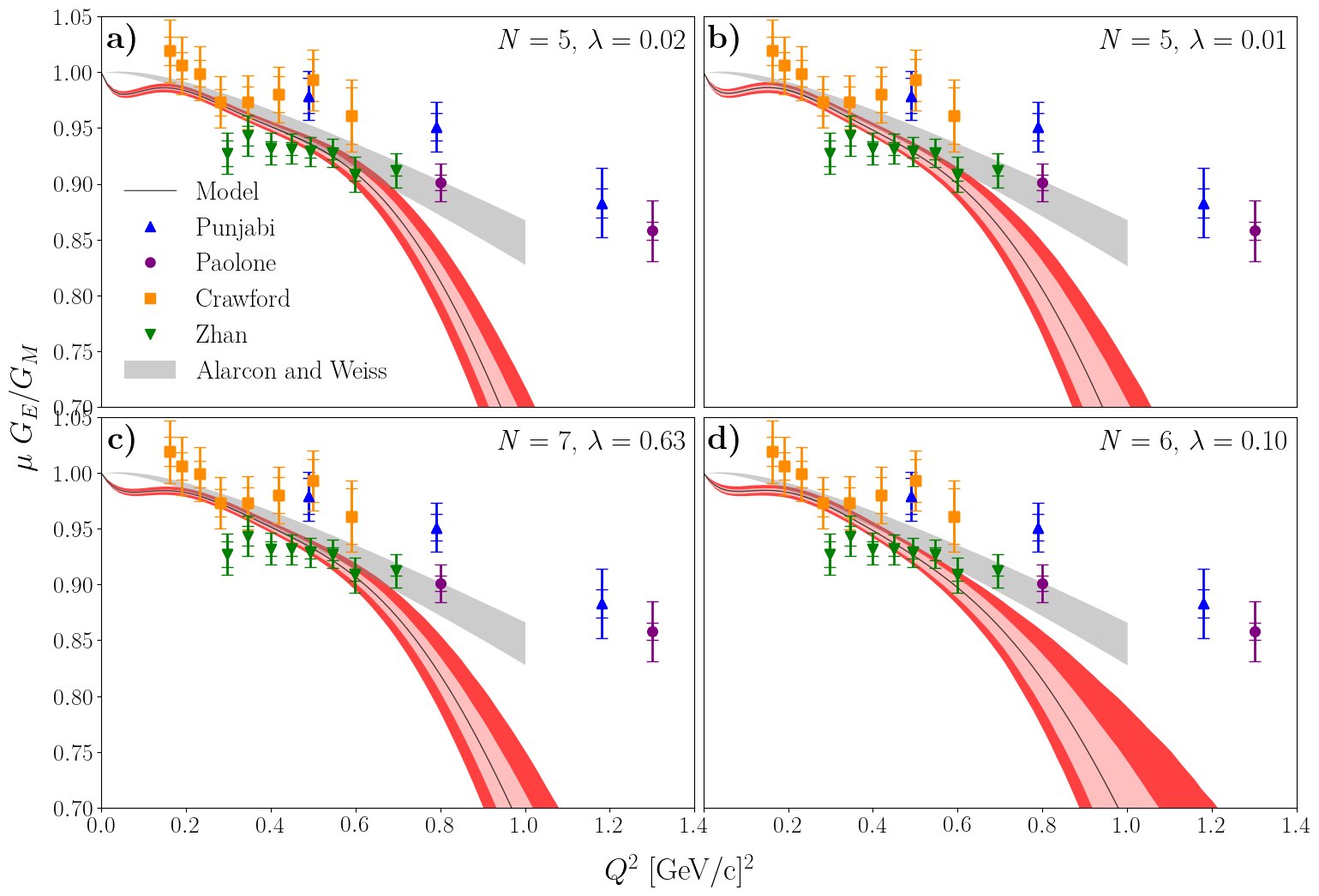
Figure 1: Ratio of the Sachs form factors as a function of $Q^{2}$. Each panel corresponds to a different data set: a) A1, b) Rebinned A1, c) A1 + PRad, d) Rebinned + PRad. Markers: asymmetry data with statistical and systematic uncertainties (consistent across all panels). Grey bands: Alarcon and Weiss’s DI$\chi$EFT model fit to the particular data set; the band is the 1$\sigma$ statistical uncertainty, propagated using a Monte Carlo method. The band is consistent across all 4 panels, as DI$\chi$EFT predicted the same model for all sets. Red bands: Gramolin and Russell’s best-fit model fit to the particular data set, with the specific order and regularization indicated in the upper right corner of the panel; the black lines are the best-fit lines, the inner, light-red bands are the 68% statistical confidence intervals and the outer, dark-red bands are the systematic uncertainties added in quadrature. The statistical bands were propagated using standard propagation of error, while the systematic bands were found by following Gramolin and Russell’s method outlined in section IV and in their PYTHON code, which itself follows the original A1 analysis; the statistical bands were also calculated using a ratio distribution [50] and a Monte Carlo method, both of which were found to be well approximated by the standard propagation.

In Figure 1, the form factor ratio is plotted for each data set’s best fit model as a function of the four momentum transfer, $Q^{2}$, together with the asymmetry data that was not included in the fit and is being used here as validation data. As is clearly exhibited, the authors’ model diverges significantly from the asymmetry data at $Q^{2}$ values larger than  0.8 $(GeV/c)^{2}$, indicating that the model does not accurately describe the ratio of the Sachs form factors.

In comparison, consider the DI$\chi$EFT theoretical framework of Alarcon & Weiss [51, 52, 53]. DI$\chi$EFT can relate a given proton charge and magnetic radius to a prediction for the $Q^{2}$ dependence of the form factors, $G_{E}(Q^{2})$ and $G_{M}(Q^{2})$, by utilizing a combination of dispersion analysis and chiral effective field theory [54, 55]. Thus, DI$\chi$EFT can serve as a form factor model with 2 parameters, $r_{E}$ and $r_{M}$, which can extract the radii values by being fit to electron scattering data.

In Ref. [54], Alarcon & Weiss fit their DI$\chi$EFT model to the same set of A1 Collaboration data that Gramolin and Russell used; they found a radius of $r_{E}=0.842\pm 0.002\text{ (1$\sigma$ fit uncertainty)}^{+0.005}_{-0.002}$ (full-range theory uncertainty) fm. Unlike Gramolin and Russell’s method, when fit to the same 3 additional data sets used in this comment, DI$\chi$EFT found radii consistent with their fit to the original A1 data. Further, as can be seen in Figure 1, Alarcon & Weiss’s model does not suddenly diverge from the asymmetry data for $Q^{2}>~{}0.8$ in the way that Gramolin and Russell’s model does.

IV Proton Magnetic Radius

In addition to the charge radius, one can also extract the magnetic radius from these same fits. While Gramolin and Russell do not explicitly extract the magnetic radius in their paper, it is straight forward to do and we have done it for each data set from their model by calculating $G_{M}$ from $Q^{2}$ at very small intervals close to zero and calculating the slope between the points closest to zero, a brute force derivative. We then use the same equation 1 replacing $G_{E}$ with $\frac{G_{M}}{\mu}$ to get the magnetic radius.

We see from those results shown in Table 10 that the extracted magnetic radius of the proton is substantially smaller than the respective extracted electric radius. In particular, the value Gramolin and Russell’s method obtains from the A1 data differs greatly from the value that the A1 collaboration themselves arrive at, which is 0.777 fm [37], despite them trying to replicate the A1 collaboration’s results.

Table 10: The magnetic radius of the proton extracted from each data set using numerically approximated derivatives.

Data Set	$r_{M}$ (fm)
Original A1	0.7462
Rebinned A1	0.7380
A1 + PRad	0.7702
Rebinned + PRad	0.7557

V Conclusions

When using the proton radius extraction procedure from Gramolin and Russel [44] with different sets of electron scattering data, we find that results are not consistent. In fact, even a re-binning of the same data results in a vastly different extracted radius. We also note that while this method exploited the known $Q^{2}$ limiting, it still failed to extrapolate beyond the data that was included in the fits. Thus we find that this method is not robust and that the strong conclusions about a particular proton radius that the authors claimed are not justified.

References

- Hofstadter and McAllister [1955] R. Hofstadter and R. W. McAllister, Phys. Rev. 98, 217 (1955).
- Hand et al. [1963] L. N. Hand, D. G. Miller, and R. Wilson, Rev. Mod. Phys. 35, 335 (1963).
- Frerejacque et al. [1966] D. Frerejacque, D. Benaksas, and D. J. Drickey, Phys. Rev. 141, 1308 (1966).
- Akimov et al. [1972] Y. K. Akimov et al., Sov. Phys. JETP 35, 651 (1972).
- Murphy et al. [1974] J. J. Murphy, Y. M. Shin, and D. M. Skopik, Phys. Rev. C 9, 2125 (1974), [Erratum: Phys.Rev.C 10, 2111–2111 (1974)].
- Borkowski et al. [1975a] F. Borkowski, P. Peuser, G. G. Simon, V. H. Walther, and R. D. Wendling, Nucl. Phys. B 93, 461 (1975a).
- Borkowski et al. [1975b] F. Borkowski, G. G. Simon, V. H. Walther, and R. D. Wendling, Z. Phys. A 275, 29 (1975b).
- Hohler et al. [1976] G. Hohler, E. Pietarinen, I. Sabba Stefanescu, F. Borkowski, G. G. Simon, V. H. Walther, and R. D. Wendling, Nucl. Phys. B 114, 505 (1976).
- Simon et al. [1980] G. G. Simon, C. Schmitt, F. Borkowski, and V. H. Walther, Nucl. Phys. A 333, 381 (1980).
- McCord et al. [1991] M. McCord, H. Crannell, L. W. Fagg, J. T. O’Brien, D. I. Sober, J. W. Lightbody, X. K. Maruyama, and P. A. Treado, Nucl. Instrum. Meth. B56/57, 496 (1991).
- Wong [1994] C. W. Wong, Int. J. Mod. Phys. E 3, 821 (1994).
- Mergell et al. [1996] P. Mergell, U. G. Meissner, and D. Drechsel, Nucl. Phys. A 596, 367 (1996), arXiv:hep-ph/9506375 .
- Rosenfelder [2000] R. Rosenfelder, Phys. Lett. B 479, 381 (2000), arXiv:nucl-th/9912031 .
- Gough Eschrich et al. [2001] I. M. Gough Eschrich et al. (SELEX), Phys. Lett. B 522, 233 (2001), arXiv:hep-ex/0106053 .
- Sick [2003] I. Sick, Phys. Lett. B 576, 62 (2003), arXiv:nucl-ex/0310008 .
- Kelly [2004] J. J. Kelly, Phys. Rev. C 70, 068202 (2004).
- Blunden and Sick [2005] P. G. Blunden and I. Sick, Phys. Rev. C 72, 057601 (2005), arXiv:nucl-th/0508037 .
- Belushkin et al. [2007] M. A. Belushkin, H. W. Hammer, and U. G. Meissner, Phys. Rev. C 75, 035202 (2007), arXiv:hep-ph/0608337 .
- Hill and Paz [2010] R. J. Hill and G. Paz, Phys. Rev. D 82, 113005 (2010).
- Borisyuk [2010] D. Borisyuk, Nucl. Phys. A 843, 59 (2010), arXiv:0911.4091 [hep-ph] .
- Bernauer et al. [2010] J. C. Bernauer, P. Achenbach, C. Ayerbe Gayoso, R. Böhm, D. Bosnar, L. Debenjak, M. O. Distler, L. Doria, A. Esser, H. Fonvieille, J. M. Friedrich, J. Friedrich, M. Gómez Rodríguez de la Paz, M. Makek, H. Merkel, D. G. Middleton, U. Müller, L. Nungesser, J. Pochodzalla, M. Potokar, S. Sánchez Majos, B. S. Schlimme, S. Širca, T. Walcher, and M. Weinriefer (A1 Collaboration), Phys. Rev. Lett. 105, 242001 (2010).
- Ron et al. [2011] G. Ron et al. (Jefferson Lab Hall A), Phys. Rev. C 84, 055204 (2011), arXiv:1103.5784 [nucl-ex] .
- Zhan et al. [2011] X. Zhan et al., Phys. Lett. B 705, 59 (2011), arXiv:1102.0318 [nucl-ex] .
- Sick [2012] I. Sick, Prog. Part. Nucl. Phys. 67, 473 (2012).
- Adamuscin et al. [2012] C. Adamuscin, S. Dubnicka, and A. Z. Dubnickova, Prog. Part. Nucl. Phys. 67, 479 (2012).
- Lorenz et al. [2012] I. T. Lorenz, H. W. Hammer, and U.-G. Meissner, Eur. Phys. J. A 48, 151 (2012), arXiv:1205.6628 [hep-ph] .
- Graczyk and Juszczak [2014] K. M. Graczyk and C. Juszczak, Phys. Rev. C 90, 054334 (2014), arXiv:1408.0150 [hep-ph] .
- Lorenz et al. [2015] I. T. Lorenz, U.-G. Meißner, H. W. Hammer, and Y. B. Dong, Phys. Rev. D 91, 014023 (2015), arXiv:1411.1704 [hep-ph] .
- Arrington and Sick [2015] J. Arrington and I. Sick, J. Phys. Chem. Ref. Data 44, 031204 (2015), arXiv:1505.02680 [nucl-ex] .
- Lee et al. [2015] G. Lee, J. R. Arrington, and R. J. Hill, Phys. Rev. D 92, 013013 (2015), arXiv:1505.01489 [hep-ph] .
- Griffioen et al. [2016] K. Griffioen, C. Carlson, and S. Maddox, Phys. Rev. C 93, 065207 (2016).
- Higinbotham et al. [2016] D. W. Higinbotham, A. A. Kabir, V. Lin, D. Meekins, B. Norum, and B. Sawatzky, Phys. Rev. C 93, 055207 (2016).
- Horbatsch et al. [2017] M. Horbatsch, E. A. Hessels, and A. Pineda, Phys. Rev. C 95, 035203 (2017).
- Alarcón et al. [2019a] J. M. Alarcón, D. W. Higinbotham, C. Weiss, and Z. Ye, Phys. Rev. C 99, 044303 (2019a).
- Zhou et al. [2019] S. Zhou, P. Giulani, J. Piekarewicz, A. Bhattacharya, and D. Pati, Phys. Rev. C 99, 055202 (2019).
- Xiong et al. [2019] W. Xiong et al., Nature 575, 147 (2019).
- Alarcón et al. [2020a] J. M. Alarcón, D. W. Higinbotham, and C. Weiss, Phys. Rev. C 102, 035203 (2020a).
- Hayward and Griffioen [2020] T. B. Hayward and K. A. Griffioen, Nucl. Phys. A 999, 121767 (2020), arXiv:1804.09150 [nucl-ex] .
- Mihovilovič et al. [2021] M. Mihovilovič et al., Eur. Phys. J. A 57, 107 (2021), arXiv:1905.11182 [nucl-ex] .
- Atac et al. [2021] H. Atac, M. Constantinou, Z. E. Meziani, M. Paolone, and N. Sparveris, Eur. Phys. J. A 57, 65 (2021), arXiv:2009.04357 [nucl-ex] .
- Lin et al. [2021] Y.-H. Lin, H.-W. Hammer, and U.-G. Meißner, Phys. Lett. B 816, 136254 (2021), arXiv:2102.11642 [hep-ph] .
- Cui et al. [2021] Z.-F. Cui, D. Binosi, C. D. Roberts, and S. M. Schmidt, Phys. Rev. Lett. 127, 092001 (2021).
- Lin et al. [2022] Y.-H. Lin, H.-W. Hammer, and U.-G. Meißner, Phys. Rev. Lett. 128, 052002 (2022).
- Gramolin and Russell [2022] A. V. Gramolin and R. L. Russell, Phys. Rev. D 105, 054004 (2022), arXiv:2102.13022 [nucl-ex] .
- Bernauer et al. [2014] J. C. Bernauer, M. O. Distler, J. Friedrich, T. Walcher, P. Achenbach, C. Ayerbe Gayoso, R. Böhm, D. Bosnar, L. Debenjak, L. Doria, A. Esser, H. Fonvieille, M. Gómez Rodríguez de la Paz, J. M. Friedrich, M. Makek, H. Merkel, D. G. Middleton, U. Müller, L. Nungesser, J. Pochodzalla, M. Potokar, S. Sánchez Majos, B. S. Schlimme, S. Širca, and M. Weinriefer (A1 Collaboration), Phys. Rev. C 90, 015206 (2014).
- Note [1] The dagger () signifies slight differences in rounding based on different IDE’s and computers.
- Punjabi et al. [2005] V. Punjabi et al., Phys. Rev. C 71, 055202 (2005), [Erratum: Phys.Rev.C 71, 069902 (2005)], arXiv:nucl-ex/0501018 .
- Crawford et al. [2007] C. B. Crawford et al., Phys. Rev. Lett. 98, 052301 (2007), arXiv:nucl-ex/0609007 .
- Paolone et al. [2010] M. Paolone et al., Phys. Rev. Lett. 105, 072001 (2010), arXiv:1002.2188 [nucl-ex] .
- Hinkley [1969] D. V. Hinkley, Biometrika 56, 635 (1969).
- Alarcón and Weiss [2017] J. M. Alarcón and C. Weiss, Phys. Rev. C 96, 055206 (2017), arXiv:1707.07682 [hep-ph] .
- Alarcón and Weiss [2018a] J. M. Alarcón and C. Weiss, Phys. Rev. C 97, 055203 (2018a), arXiv:1710.06430 [hep-ph] .
- Alarcón and Weiss [2018b] J. M. Alarcón and C. Weiss, Phys. Lett. B 784, 373 (2018b), arXiv:1803.09748 [hep-ph] .
- Alarcón et al. [2020b] J. M. Alarcón, D. W. Higinbotham, and C. Weiss, Phys. Rev. C 102, 035203 (2020b), arXiv:2002.05167 [hep-ph] .
- Alarcón et al. [2019b] J. M. Alarcón, D. W. Higinbotham, C. Weiss, and Z. Ye, Phys. Rev. C 99, 044303 (2019b), arXiv:1809.06373 [hep-ph] .