On the nature of disks at high redshift seen by JWST/CEERS with contrastive learning and cosmological simulations

Abstract

Visual inspections of the first optical rest-frame images from JWST have indicated a surprisingly high fraction of disk galaxies at high redshifts. Here, we alternatively apply self-supervised machine learning to explore the morphological diversity at $z\geq 3$. Our proposed data-driven representation scheme of galaxy morphologies, calibrated on mock images from the TNG50 simulation, is shown to be robust to noise and to correlate well with the physical properties of the simulated galaxies, including their 3D structure. We apply the method simultaneously to F200W and F356W galaxy images of a mass-complete sample ($M_{*}/M_{\odot}>10^{9}$) at $3\leq z\leq 6$ from the first JWST/NIRCam CEERS data release. We find that the simulated and observed galaxies do not exactly populate the same manifold in the representation space from contrastive learning. We also find that half the galaxies classified as disks —either CNN-based or visually— populate a similar region of the representation space as TNG50 galaxies with low stellar specific angular momentum and non-oblate structure. Although our data-driven study does not allow us to firmly conclude on the true nature of these galaxies, it suggests that the disk fraction at $z\geq 3$ remains uncertain and possibly overestimated by traditional supervised classifications. Deeper imaging and spectroscopic follow-ups as well as comparisons with other simulations will help to unambiguously determine the true nature of these galaxies, and establish more robust constraints on the emergence of disks at very high redshift.

1 Introduction

Understanding how galaxy diversity emerges across cosmic time is one of the main goals of galaxy formation. How and when do stellar disks form? What are the main drivers of bulge growth? How and when did galaxy morphology and star formation get connected? Despite significant progress in the past years, thanks in particular to deep surveys undertaken with the Hubble Space Telescope (HST, e.g., Scoville et al., 2007; Grogin et al., 2011a; Koekemoer et al., 2011), these questions remain largely unanswered. The general picture is that massive star-forming galaxies in the past were more irregular in their stellar structure (e.g., Abraham et al., 1996; Conselice, 2003) than today’s disks even if observed in the optical rest-frame (Buitrago et al., 2013; Huertas-Company et al., 2015). Galaxies above $z\sim 1$ also show the presence of giant star-forming clumps (e.g, Guo et al., 2015, 2018; Huertas-Company et al., 2020; Ginzburg et al., 2021) which might indicate a turbulent and unstable Interstellar Medium (ISM, e.g., Ceverino et al., 2010; Bournaud et al., 2014). Although the gas shows signatures of rotation at $z\sim 2$ (e.g.,Wisnioski et al., 2015), the settling of disks seems to be a process happening at least from $z\sim 2$ (e.g., Kassin et al., 2012; Buitrago et al., 2014; Simons et al., 2017; Costantin et al., 2022) coincident with the decrease of gas fractions in massive galaxies (e.g., Freundlich et al., 2019; Genzel et al., 2010). Another important result of the past years is that the presence of bulges in galaxies is strongly anti-correlated with the star formation activity at all redshifts probed (e.g., van der Wel et al., 2014a; Barro et al., 2017; Costantin et al., 2020, 2021; Dimauro et al., 2022). This suggests that bulge formation and quenching are tightly connected physical processes (e.g., Chen et al., 2020b).

With its unprecedented sensitivity, spatial resolution, and infrared coverage, the James Webb Space Telescope (JWST) is offering a new window to the stellar structure of galaxies in the first epochs of cosmic history (Gardner et al., 2006). For the first time, we are able to explore the stellar morphologies of the first galaxies formed in the universe, which should enable new constraints on the physical processes governing galaxy assembly at early times and hopefully a better understanding of the physical processes leading to the formation of the first stellar disks and bulges. Some very recent works have already started this exploration by performing visual classifications (Ferreira et al., 2022, 2023; Kartaltepe et al., 2023), by applying supervised Machine Learning trained on HST images (Robertson et al., 2023) of galaxies observed in the first JWST deep fields or by using Convolutional Neural Networks (CNNs) trained on HST/WFC3 labeled images and domain-adapted to JWST/NIRCam (Huertas-Company et al., 2023b). One of the main results of these early works is that JWST seems to be detecting star-forming disks even at $z>3$, which would push the time of disk formation to very early epochs. Two questions naturally arise from these first works:

• Are the galaxies seen by JWST true disks, i.e. flat, rotating systems? The aforementioned results are based primarily on qualitative morphological classifications, with quantitative tracers of morphology (e.g., Sèrsic fits) incorporated to further inform differences between the visually defined classes. However, galaxies might look morphologically disky but have significantly different stellar kinematics than local disk galaxies. Distinguishing edge-on flat disks from more prolate systems is also a very challenging task that could bias the results (e.g. van der Wel et al., 2014b; Zhang et al., 2019).

• Do modern cosmological simulations reproduce the observed galaxy diversity at $z>3$? Although some preliminary comparisons exist, a fair comparison in the observational plane is required to fully address this question (e.g., Rodriguez-Gomez et al., 2019; Huertas-Company et al., 2019; Zanisi et al., 2021).

In this work, we attempt to provide new insights into these two main questions. To that purpose, we apply a novel data-driven approach based on contrastive learning (Hayat et al., 2021; Sarmiento et al., 2021) to a mass-complete sample of JWST galaxies at $z\geq 3$ observed within the Cosmic Evolution Early Release Science (CEERS; Finkelstein et al., 2017, 2022, 2023) survey. By calibrating the method with mock galaxies (Costantin et al., 2023) from the TNG50 cosmological simulation (Nelson et al., 2019a; Pillepich et al., 2019; Nelson et al., 2019b) and by choosing the proper augmentations (i.e., transformations applied to the images such as rotations, flux normalizations, noise, etc.), we are able to build a morphological description which is more robust to noise and galaxy orientation than more traditional approaches. Our morphological representation can then be correlated with the physical properties of galaxies from the simulation to provide new insights about the physical nature of disk-like galaxies, and to explore the agreements and disagreements between observations and simulations.

The paper proceeds as follows: in section 2 we describe the galaxy datasets used in this work; section 3 describes the contrastive learning setting used to derive unsupervised representations of galaxy morphologies; section 4 explores the properties of the obtained representations on observed JWST/CEERS galaxies; a comparison of the self-supervised representations for simulated and observed galaxies is presented in section 5; the results and implications are discussed in section 6; finally, a summary and the final conclusions are presented in section 7.

2 Data

2.1 CEERS

We use JWST imaging data from NIRCam obtained within CEERS (Finkelstein et al., 2017, 2022, 2023). This consists of short and long-wavelength images in both NIRCam A and B modules, taken over ten pointings. Each pointing was observed with seven filters: F115W, F150W, and F200W on the short-wavelength side, and F277W, F356W, F410M, and F444W on the long-wavelength side. Here we only use the F200W and F356W filters. A full description of this public data release and the data reduction can be found in Bagley et al. (2023) and Finkelstein et al. (2022).

In addition to the galaxy images, we use two different catalogs with physical properties of galaxies:

• CEERS catalog (CEERS): a photometric catalog (Bagley et al., 2023; Finkelstein et al., 2022) with derived stellar masses and photometric redshifts ($z_{\mathrm{phot}}$) obtained through Spectral Energy Distribution (SED) fitting of the latest data reduction photometry (Pablo G. Pérez-González private communication). For a fair comparison with the simulated TNG50 dataset (see subsection 2.2), we select 1 664 galaxies with $3\leq z\leq 6$, stellar masses $M_{*}\geq 10^{9}\mathrm{M_{\odot}}$ and $F200W[AB]<27~{}\mathrm{mag}$. The magnitude cut ensures a large enough Signal-to-Noise Ratio (SNR) to enable reliable morphological classification (see Kartaltepe et al. 2023). Obvious stars are removed using the same procedure as in Huertas-Company et al. (2023b). Also in Huertas-Company et al. (2023b), the completeness limit is estimated at roughly $M_{*}\sim 10^{8.5}\mathrm{M_{\odot}}$ over the $0<z<6$ redshift range. The cut in mass imposed of $M_{*}\geq 10^{9}\mathrm{M_{\odot}}$ is well above this completeness limit and, therefore, the main conclusions presented hereafter in this study should not be affected by incompleteness. For the galaxies in this dataset, we also use the CNN-based morphological classifications that split them into four classes: spheroids (Sph), Bulge + Disk, Disk and disturbed (Irr). See Huertas-Company et al. 2023b, for more details.

• Visual classification catalog (VISUAL): a redshift-selected $z\geq 3$ morphological catalog presented in Kartaltepe et al. (2023) containing 850 galaxies in common between CANDELS (Grogin et al., 2011b; Koekemoer et al., 2011) and CEERS observations. This is intended to directly compare our morphological description to the visual classification of Kartaltepe et al. (2023). Redshifts and stellar masses are extracted from CANDELS v2 for the HST F160W-selected galaxies in the EGS field (see Kodra et al., 2023, for full details on the photometric redshift measurements and resulting catalogs). The visual classifications presented in Kartaltepe et al. (2023) of each galaxy are performed by three people. A given classification is assigned if two out of three people select that option. Galaxies classified in this way are broken down into the following morphological groups: Disk only, Disk+Spheroid, Disk+Irregular, Disk+Spheroid+Irregular, Spheroid only, Spheroid+Irregular and Irregular only. See Kartaltepe et al. (2023) for more details on the different classification tasks and morphological groups. After selecting those galaxies with $M_{*}\geq 10^{9}\mathrm{M_{\odot}}$, $3<z<6$, and reliable visual classifications we end up with a dataset of 545 galaxies.

Both catalogs also include morphological measurements of Sèrsic index ($n_{e}$), semi-major axis ($a$) and axis-ratio ($b/a$) derived with galfit (Peng et al., 2010). More information about the fits can also be found in Kartaltepe et al. (2023).

The distributions of stellar masses of the galaxies in the CEERS and the VISUAL datasets are shown in Figure 1. The number of galaxies at the different redshifts analyzed is shown in Table 1.

2.2 Mock JWST images of TNG50 galaxies

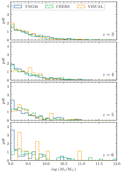
Figure 1: Probability density function of the logarithm of the stellar mass of the simulated galaxies in the TNG50 dataset (blue histogram), and the observed galaxies in the CEERS and VISUAL datasets (green and orange dashed histogram, respectively). Different panels correspond to the redshifts analyzed, $z=(3,4,5,6)$.

We use the TNG50-1 suite of simulation (hereafter TNG50; Nelson et al. 2019a; Pillepich et al. 2019; Nelson et al. 2019b) and their mock NIRCam observations at $z>3$ galaxies following the observational strategy of CEERS. The mock images were produced by modeling the gas cells and star particles in the simulation as presented in Costantin et al. (2023). We consider four snapshots of the TNG50 simulation corresponding to $z=(3,4,5,6)$ and galaxies with stellar masses $M_{*}\geq 10^{9}\mathrm{M_{\odot}}$. In total, the original dataset consists of 1 326 galaxies (see Table 1). Each selected galaxy is then observed along 20 different line-of-sight orientations to increase the statistics which produces a dataset of 26 520 galaxy images that we consider as independent objects for the purpose of this work. As described in Costantin et al. (2023), parametric and non-parametric morphological parameters for this dataset are derived using the standard configuration of statmorph(Rodriguez-Gomez et al., 2019).

For this study, we use the noiseless images in the F200W and F356W bands from the Costantin et al. (2023) dataset with a pixel scale of 0.031 and 0.063 arcsec pix^-1, respectively. We decided to use these two filters simultaneously since they probe the UV, optical, and near-IR rest-frame at $z>3$ (see Figure 2 in Ferreira et al. 2022), allowing to probe simultaneously the distribution of young and old stars and offering a complete view of galaxy morphology for our data-driven approach. Another reason for including the F200W is its spatial resolution. The F200W filter is the filter with the longest wavelength at the 0.031 arcsec pix^-1 resolution of the NIRCam short wavelength channels (F115W and F150W). Although re-sampled into the 0.031 arcsec pix^-1 resolution after drizzling, the NIRCam long wavelength channels (F277W, F356W, F410W, and F444W) a worse spatial resolution (originally 0.063 arcsec pix^-1 resolution) than the NIRCam short wavelength channels.

The original field of view of each image is twice the total half-mass radius (i.e., dark matter, gas, and star particles included) of the corresponding galaxy. This roughly corresponds to a field of view 10 times larger than the stellar half-mass radius (i.e., only star particles included). However, our image classification scheme requires a fixed image size. Therefore, we select galaxy images with a field-of-view larger than $64\times 64$ and $32\times 32$ pixels in the F200W and F356W bands, respectively, and generate cutouts of those sizes. Then, to match both observations of the same galaxy, images in the F356W band are re-sampled to the same pixel scale as the F200W images (see subsection 3.2, for more details). Given the original field of view of each galaxy image, after cutting them to the input fixed size of our network ($64\times 64$ pixels), the cutouts will certainly include all the luminous matter in the stamps.

According to these criteria, $\lesssim 7\%$ of the galaxies (most of them at $z=3$) are dropped out from our initial sample. The total number of galaxies considered is finally 1 238 distributed within $z=3-6$ (see Table 1), which translates into 24 760 projections. Although the number of objects we remove is small, we check in Figure 2 if a specific population is systematically excluded. The figure shows the size-mass relation of the selected TNG50 dataset along with the excluded galaxies based on the size of the field of view. The excluded galaxies are not necessarily the most compact and/or less massive galaxies in the dataset. However, a fraction of them with lower-than-average stellar extent is indeed removed based on our selection and would reach otherwise sizes of a few hundred parsecs.

For comparison, we show in Figure 1 the distribution of the stellar masses in the simulated TNG50 dataset, and the observed CEERS and VISUAL datasets. Note the good agreement between the TNG50 and the CEERS samples, even if we are comparing here the stellar masses directly extracted from the TNG50 simulations and those obtained through SED fitting of the latest JWST data. Also remarkable is the agreement, despite the selection effects, between the CEERS, VISUAL, and TNG50 datasets.

Table 1: Summary of the sample of TNG50 simulated galaxies and CEERS observed galaxies with $M_{*}\geq 10^{9}\mathrm{M_{\odot}}$. The first column indicates the redshift ($z$); the second column shows the total number of galaxies in the simulated TNG50 dataset; the third column refers to the number of selected galaxies according to image size limitations (i.e., $64\times 64$ and $32\times 32$ pixels in the F200W and F356W bands, respectively); the fourth column shows the number of galaxies in the CEERS dataset; the fifth column indicates the number of galaxies in the VISUAL dataset. Note that for the CEERS and VISUAL datasets galaxies are split into the following redshift bins: $z=3$ for $3.0\leq z<3.5$, $z=4$ for $3.5\leq z<4.5$, $z=5$ for $4.5\leq z=5.5$ and $z=6$ for $5.5\leq z<6.0$.

$z$	TNG50	TNG50	CEERS	VISUAL
	(All)	(Selected)
3-6	1326	1238	1664	545
3	829	760	741	216
4	343	326	463	201
5	115	113	398	119
6	39	39	62	9

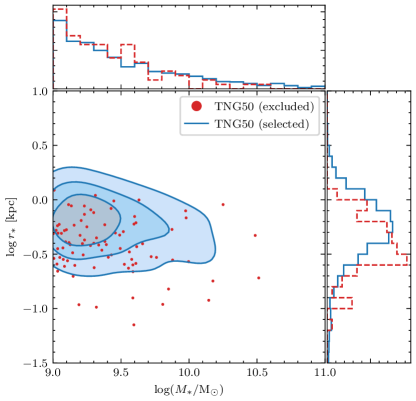
Figure 2: Logarithm of the physical size (stellar half-mass radius, $r_{*}$, in kpc) versus the stellar mass ($M_{*}$, in $\mathrm{M_{\odot}}$) of the TNG50 galaxies. Blue-filled contours show the $25\%$, $50\%$, and $75\%$ probabilities of the TNG50 selected galaxies. Red data points correspond to the excluded galaxies in terms of the size of the field-of-view. See Table 1.

3 Self-supervised learning representation of mock JWST images of simulated TNG50 galaxies

In this section, we describe the main methodology we developed to obtain a data-driven morphological description of galaxies that is robust to noise and other nuisance parameters.

3.1 Contrastive learning framework

Our approach is based on an adaptation of the Simple framework for Contrastive Learning of visual Representations (SimCLR; Chen et al., 2020a). Very briefly, the idea behind the SimCLR framework is to obtain robust representations of images without labels by applying random augmentations as explained below. See Huertas-Company et al. (2023a), for a recent review of this technique applied to Astrophysics.

Given an image, random transformations are applied to it to generate a pair of two augmented images, $(x_{i},x_{j})$. Each image in the pair is passed through a Convolutional Neural Network (CNN) to compress the images into a set of vectors, $(h_{i},h_{j})$. Then, a non-linear fully connected layer (i.e., projection head) is placed to get the representations $(z_{i},zj)$. The representations are learned iteratively by maximizing agreement between the augmented views of the same image example $(z_{i},zj)$ and minimizing agreement between all other pairs considered as negatives. This is achieved via a so-called contrastive loss in the latent space:

$$l_{i,j}=-\log\frac{\exp(\langle\boldsymbol{z}_{i},\boldsymbol{z}_{j}\rangle/h)}{\Sigma_{k=1,k\neq i}^{2N}\,\,\exp(\langle\boldsymbol{z}_{i},\boldsymbol{z}_{k}\rangle/h)},$$ (1)

where $\langle\boldsymbol{u},\boldsymbol{v}\rangle$ denotes the dot product between $L^{2}$-normalized $\boldsymbol{u}$ and $\boldsymbol{v}$, and $h$ denotes the temperature parameter that regulates the distribution of the output representations (see Hinton et al., 2015; Wu et al., 2018, for more details). The final loss is computed in batches of size $N$ across all positive pairs, both $(i,j)$ and $(j,i)$, while the rest of the augmented examples are treated as negative examples, which are denoted by $k$.

For this study, we follow the implementation from Sarmiento et al. (2021), which was successfully applied to astronomical data. The CNN encoder consists of four convolutional layers with kernel sizes 5, 3, 3, 3, and 128, 256, 512, and 1 024 filters per layer, respectively. Max-pooling layers and Exponential Linear Unit (ELU) activation functions are placed after each convolutional layer. Therefore, the representations before the projection head —$(h_{i},h_{j})$— for each galaxy image are encoded into 1 024 features. Subsequently, the projection head (composed of three fully connected layers of 512, 128, and 64 neurons per layer) transforms the galaxy representations to a latent space —$(z_{i},z_{j})$— where the contrastive loss is computed.

3.2 Data augmentation and network training

The choice of data augmentations is a key element in contrastive learning training (Chen et al., 2020a) as it allows us to turn the representations independent of some nuisance effects. In the context of this study, our goal is to obtain a morphological representation that is robust to signal-to-noise, rotation, and size, and does not depend on color. To reach this objective, we calibrate our algorithm on the mock TNG50 dataset (subsection 2.2) since it allows us to access noiseless versions of the images and, therefore, marginalize the noise.

For each simulated TNG50 galaxy image, we produce two augmented images ($x_{i},x_{j}$) from the noiseless version. One of the images from the pair —the one used to produce the noise-added image— is then convolved by the corresponding PSF in each filter (extracted from the observations Finkelstein et al. 2022 in each band), while the other image —the one used to produce the noiseless image— is not convolved by the PSF to keep as much as spatial information as possible. Both images are re-scaled in flux (as described below) independently. Then, we add source Poisson noise only to the image used for the noise-added version. To match the same pixel scale in the two filters, we then re-bin the images in the F356W filter to the same pixel scale as the images in the F200W filter. Finally, for the noise-added image, we include realistic noise by adding random patches of the sky extracted from the 10 CEERS pointings. Below we described more precisely the augmentations applied to the images:

• Rotation: we first apply a random flipping (horizontal or vertical, but not both) and a random rotation with 100% chance independently to the TNG50 noiseless image and the patch of the sky extracted from the CEERS pointings. Also the noiseless and the noise-added version are rotated and flipped differently. This augmentation is intended to ensure the model is invariant to the galaxy orientation;

• Flux: we randomly apply flux scaling to the noise-added version of the images after the PSF convolution, but before noise is added. The flux factor applied to the noise-added images in the two filters is randomly sampled from the flux distribution of the TNG50 dataset in the F356W band. The same flux factor is applied to both the F200W and F356W filters. This augmentation is intended to stress the robustness to S/N. It may also help —as we will show in the following— to make the representations independent of galaxy size since the regions above the noise level will vary with the flux variations.

• Noise: as described in section 2, for each galaxy image in the F200W and F356W bands we have a noiseless version that does not include any instrumental effects or noise. Using the available CEERS data, we construct mock CEERS galaxy images as a combination of the TNG50 noiseless images and random patches of the ten observed CEERS pointings. For the noise-added version, we first add source Poisson noise and, then, we add real-time realistic noise (that may also include other sources/interlopers) to each of the $64\times 64$ noiseless galaxy images by summing up one randomly chosen patch (different in each augmentation) from the CEERS pointing of the same size. From the contrastive learning point of view, these images with a real background are considered as an augmented copy of their noiseless analogs during the training process. These augmentations should enforce the representations to be robust to signal-to-noise (S/N) as well as to background and foreground companions.

• Color: finally, in order to prevent the network from learning color information and/or the intrinsic brightness of the galaxies directly from the images, we apply two additional augmentations to both the noiseless and the noise-added images. First, each band is normalized individually after the augmentations are applied. Second, the noiseless and noise-added images are normalized independently and individually for each galaxy. Consequently, the maximum pixel value in every galaxy image (both noiseless and noise-added) is equal to one for each band.

We note that we decided not to apply direct size augmentation, (i.e. such as zoom-in or zoom-out), as that would force us to up-sample or down-sample the images with less or more than $64\times 64$ pixels size, respectively, which creates some artifacts that the network is able to learn. The choice of the cutouts’ size when producing the galaxy images is always complicated. One might prefer to make the stamps proportional to the size of the galaxy (see Vega-Ferrero et al. 2021, for an example). However, that requires reliable measurements of the galaxy sizes and also the re-sampling of the cutouts to the same size in pixels. Contrarily, it is possible to produce all the cutouts with the same size in pixels, independently of the galaxy size. By doing so, it is not needed to re-sample the cutouts since they already have the same dimensions. We decide to use a fixed size for the cutout to avoid: first, artifacts and noise correlations originating from the re-sampling phase that could mislead the contrastive learning representations; and second, losing spatial resolution of galaxies with large sizes after the re-sampling phase.

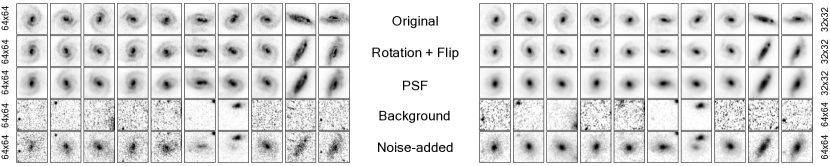
Figure 3: Images and augmentations of a TNG50 galaxy at $z=3$ with $M_{*}\approx 6\times 10^{9}\mathrm{M_{\odot}}$ in the F200W (left-hand panel) and F356W (right-hand panel) filters. The different rows (from top to bottom) correspond to: the original/noiseless image; the original image after rotation and flipping (vertical or horizontal); the image after PSF convolution; the background CEERS patch of the sky; the noise-added image, i.e., the sum of the PSF convolved image (flux variation and source Poisson noise applied) and the background patch of the sky. All the panels have a $64\times 64$ pixels size, except the first three rows for the F356W filter that have the original size of $32\times 32$ pixels before re-binning to $64\times 64$ pixels. The pixel values have been $asinh$ transformed with a 0.5% clipping.

In Figure 3, we show several projections of a galaxy at $z=3$ with $M_{*}\approx 6\times 10^{9}\mathrm{M_{\odot}}$ extracted from the TNG50 simulation. In some of the augmented versions (along with PSF convolution, realistic noise, random rotations, flux variation, etc.), it is possible to distinguish several companions within the stamps. This is the result of adding randomly chosen patches of the CEERS pointings to the TNG50 noiseless images. These examples come from an extended bright galaxy that appears significantly dimmer in some of the augmented images due to the flux variations applied in the augmentations. In summary, the contrastive model should be able to extract a meaningful representation $(h_{i},h_{j})$ that minimizes the distance between the representations $(z_{i},z_{j})$ of the two images (original/noiseless and noise-added) of the same galaxy, even if they appear as different as shown in some panels in Figure 3.

Our contrastive SimCLR model is trained and tested with the mock JWST images for 24 760 different projections of 1 238 galaxies within $3\leq z\leq 6$ and with stellar masses $M_{*}\geq 10^{9}\mathrm{M_{\odot}}$ in the two observed bands (F200W and F356W) with a temperature parameter $h=0.5$ (that controls the strength of penalties on hard negative pairs). We randomly split our dataset into a training and a test sample consisting of 1 100, and 138 galaxies, respectively. This translates into a training and a test dataset of 22 000 and 2 760 galaxy images, respectively. None of the projections of the galaxies in the test set has ever passed through the network during training. Additionally, we ensure that only one projection of the same galaxy enters each batch during training and that all the galaxy images are passed through the network at every epoch. We do so to avoid the algorithm learning the orientation of the same galaxy as seen from different line-of-sight projections since some of the projections are just a simple rotation of the galaxy in the sky.

The input tensors in our contrastive model have, therefore, a dimension of $(N,64,64,2)$, with N being the batch size, 64 and 64 being the dimensions of the input images, and 2 the number of channels or filters (i.e., the F200W and the F356W images). We train our algorithm with a batch size of $N=550$ (i.e., half the number of galaxies in the training set) for 1 500 epochs in a GPU NVIDIA T4 Tensor Core with 16 GB of RAM. Random data augmentation is applied every 50 epochs and, therefore, we produce 30 ($1500/50$) different augmentations of the whole dataset to increase the variability during the training process. To reduce the dynamic range and to be sensitive to both the center and outskirts of the galaxy, before training, we apply a $asinh$ (inverse hyperbolic sin) transformation and a minimum-maximum normalization to each galaxy pair in each band.

In order to reduce the impact of possible discrepancies between the galaxies in the simulated TNG50 and observed CEERS datasets, when applying our model to data, we fine-tuned the model trained previously with a mixed dataset of simulated TNG50 and observed CEERS galaxies. By doing so, we expect the model to learn important features from the observed CEERS galaxy images that were not present in the training set consisting only of simulated TNG50 galaxy images and, therefore, mitigate possible domain drift-related effects. We fine-tune the model with a training set consisting of 1 500 images randomly extracted from the previous training set (of noiseless and noise-added images) and 1 500 images randomly selected from the CEERS dataset of 1 664 galaxy images. Note that for the observed dataset we do not have noiseless images so, we fed the model with pairs of CEERS galaxy images to which different augmentations (only flip and rotation) are applied. We fine-tune the model up to 600 epochs (enough to converge) with a batch size of $N=500$ galaxy images. In each epoch, random augmentations are applied to the observed CEERS pairs of images to increase the variability. For the simulated TNG50 images, the set of 1 500 also varies from epoch to epoch by selecting different galaxies and augmentations for each galaxy in the training TNG50 dataset, but not from the reserved test set which is always kept apart from the training.

3.3 Visualization of the representation space

Figure 4: Randomly chosen images of the simulated TNG50 galaxies in the UMAP visualization. The UMAP space is binned and one galaxy image per bin is shown. The left-hand panel shows the noiseless versions of the training galaxies, while the reduced versions (TNG50 + random CEERS patch) are shown in the right-hand panel. Extended/disky galaxies lie in the upper-right, compact/rounder galaxies are located in the bottom-left, and bright companions (only in the right-hand panel) concentrate toward the upper-left section of the UMAP plane. Note that there is not a one-to-one correspondence between the galaxies shown in the two panels. Both panels correspond to galaxy images in the F200W filter.

We can hence analyze the properties of the representation space learned by the SimCLR framework presented in the previous section.

We start by visualizing how the TNG50 galaxy images, both with and without noise, are distributed in the representation space. It should be noted that, hereafter, the difference between the noiseless and the noise-added version of the TNG50 galaxy images is only the added patch of the CEERS paintings. Apart from the realistic noise added, no other augmentations are applied in this phase (only in the training phase described in the previous section). Since the representation space for each galaxy image is encoded into 1 024 features, we perform a dimensionality reduction from the 1 024 features to a 2D space to facilitate the visualization and interpretation of this representation. For that purpose, we use the Uniform Manifold Approximation and Projection (UMAP; McInnes et al., 2018) method with standard initial parameters (metric = euclidean, n_neighbors $=15$ and min_dist $=0.1$). The UMAP algorithm seeks to learn the manifold structure of the input data and find a low-dimensional embedding that preserves the essential topological structure of that manifold. It is therefore a way to visualize in 2D the representations learned by the self-supervised network. Before applying the UMAP technique, we assume the same distance metric in the representation space as the one used to calculate the contrastive loss in the head projection space and, therefore, we normalize the representations with an $L^{2}$-norm such that the Euclidean and cosine distances between representations are equivalent. The two coordinate axes in the UMAP representation do not have any precise physical meaning and are a combination of the 1 024 dimensions extracted by the contrastive learning setting.

It is important to emphasize that the contrastive approach is not intended for dimensionality reduction but for obtaining a robust representation of galaxy morphologies in a different space than images, which explains the high dimensionality of the representation space. Several works have shown indeed that the performance of contrastive learning increases with representations of higher dimension (e.g.,Chen et al., 2020a).

In Figure 4, we show random examples of galaxies in the F200W filter (both with and without noise) in the UMAP 2D space. Note that some stamps on the right-hand panel (along with the addition of observed noise) show one (or more) foreground/background sources in the field of view. The figure clearly shows that galaxies are not randomly organized in the plane, indicating that the network has learned some relevant morphological features. The distributions are also similar for galaxies with and without noise. Galaxies with extended light distributions and with clear signs of a disk component —or interactions— tend indeed to appear on the right and upper-right parts of the UMAP space, while more compact galaxies with smoother and concentrated light distributions tend to be placed on the left section of the plane. We can also see that galaxies showing more elongated shapes are found toward the bottom-right section of the representation space. Also interesting to notice is how several galaxies with bright companions (off-center sources) tend to be placed on the upper-left of the right-half panel (see subsection 3.4 below for a more detailed discussion on this point).

3.4 A morphological description of galaxies robust to noise and background/foreground contaminants

Figure 5: Left-hand panel: UMAP visualization for all the TNG50 galaxy images in our dataset color-coded by the mean value of the distance in the UMAP representation between the noiseless and the reduced images of each galaxy (denoted as $\delta$). Right-hand panel: UMAP visualization for all the TNG50 galaxy images in our dataset color-coded by the mean value of the ratio of the flux measured in the TNG50 stamps and the flux derived from the noiseless TNG50 stamps for the F356W filter (denoted as $\delta_{\mathrm{F356W}}$). Large values of $\delta_{\mathrm{F356W}}$ indicate the presence of a secondary (or even more) source. The larger $\delta_{\mathrm{F356W}}$ is, the brighter the companions are with respect to the central galaxy.

We now examine in more detail the differences between the representations of noise-added and noiseless TNG50 galaxy images, and how the different augmentations of the same galaxy are represented by our contrastive model. As described in subsection 3.1, one of the reasons for using the SimCLR framework is to obtain a data-driven representation that is robust to noise and other observational effects such as foreground and background companions.

On one hand, we quantify the effect of noise by computing the distance in the UMAP representation between the noiseless and the noise-added images of each galaxy, denoted as $\delta$. On the other hand, we check how our contrastive model behaves when more than one source (i.e., companions) is present in the stamp. To do so we measure the total flux in the noise-added galaxy images (TNG50 + random CEERS patch) and in the noiseless TNG50 stamps (therefore, the intrinsic flux of the central galaxy after the flux scaling is applied) for the F356W filter. Then we compute the ratio of the two, denoted as $\delta_{\mathrm{F356W}}$, as a proxy for the presence (or not) of companions and, if present, how bright they are with respect to the central galaxy.

In Figure 5, we show the UMAP plane for TNG50 galaxy images in our dataset color-coded by $\delta$ and $\delta_{\mathrm{F356W}}$. For a reference of the UMAP axis ranges, the horizontal axis (UMAP 1) spans within $(0.9,12.1)$, and the vertical axis (UMAP 2) spans within $(-1.7,5.5)$. The total area covered by the data points in the UMAP plane is approximately 60 (in the arbitrary UMAP units). It is interesting to note how the main yellow clump in the upper-left section of the UMAP plane where the stamps with bright companions (more than three times the flux than the flux of the central galaxy, i.e., $\delta_{\mathrm{F356W}}\gtrsim 4$) tend to concentrate, and also their correlation with large values $\delta\gtrsim 2.5$. Some of these cases can be seen in the right-hand panel in Figure 4. For instance, there are several examples within these regions of $\delta_{\mathrm{F356W}}\gtrsim 4$ that correspond to TNG50 images for which the companion is so bright (such as a star) that the central galaxy cannot be even identified in the stamp. In these cases with bright companions around the central galaxy, the model detects the brightest component (thus, the companion) instead of the central galaxy and tends to represent it in a particular region of the UMAP plane. Additionally, in the right-hand panel, it is also clear a yellow clump with large values of $\delta_{\mathrm{F356W}}$ and moderate values of $\delta$. These cases correspond to nose-added images with a bright companion that, contrarily, are still close to their noiseless counterpart (i.e., $\delta\lesssim 2$). We inspect in detail several of these cases and find that their noiseless counterparts tend to be located on the bottom-right section of the UMAP plane. In any case, a galaxy image represented close to these regions of $\delta\gtrsim 2$ might be not well-represented and should be (at least) treated carefully or excluded from the subsequent analysis. It is also interesting to note the clump with large values of $\delta$ in the left edge of the representation space (i.e., $0.0<\mathrm{UMAP~{}1}<1.5$ and $2.0<\mathrm{UMAP~{}2}<3.5$) with no clear correlation with large values of $\delta_{\mathrm{F356W}}$. Although this clump does not include a large number of galaxies, we find that those objects have their noiseless counterparts displaced up in the UMAP plane. These are very compact galaxies that look even more compact in their noiseless versions.

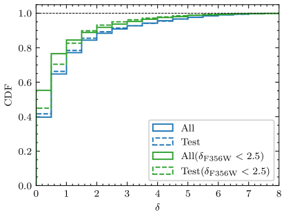
Figure 6: Cumulative distribution function of the distance in the UMAP plane between pairs of the same galaxy images, denoted as $\delta$. Blue histograms correspond to the distribution of $\delta$ for the training (solid) and the test (dashed) datasets. Green histograms correspond to the distribution of $\delta$ for the training (solid) and the test (dashed) datasets when only galaxy images with $\delta_{\mathrm{F356W}}<2.5$ are considered.

By excluding objects falling within the yellow clump shown in Figure 5 it is possible to clean our dataset (or a JWST/CEERS sample of observed galaxies) of bright companions/contaminants that could bias our contrastive learning representations. As an alternative, we build up a dataset of simulated TGN50 galaxy images that include all the possible augmentations described before but keeping a value of $\delta_{\mathrm{F356W}}<2.5$. By doing so we ensure our dataset does not include companions $1.5$ brighter (in flux) than the central galaxy. Nevertheless, these extremely bright contaminants are much rare in real CEERS observations than in our augmented set of galaxy images because, if the contaminant is so bright that it outshines the central galaxy, the galaxy would not be detected.

In Figure 6, we show the cumulative distribution function of $\delta$ for the galaxy images in the training and the test sets, both including and excluding galaxy images with $\delta_{\mathrm{F356W}}>2.5$. We find that $75\%$ and $90\%$ of the projections in the training dataset show values of $\delta\lesssim 1.5$ and $\delta\lesssim 3.0$ in the UMAP space, respectively. For the test set, $75\%$ and $90\%$ of the projections show values of $\delta\lesssim 1.4$ and $\delta\lesssim 2.7$ in the UMAP space, respectively. If we now exclude galaxy images with $\delta_{\mathrm{F356W}}>2.5$: for the training dataset, $75\%$ and $90\%$ of the projections show values of $\delta\lesssim 1.2$ and $\delta\lesssim 2.4$ in the UMAP space, respectively; while for the test dataset, $75\%$ and $90\%$ of the projections show values of $\delta\lesssim 1.3$ and $\delta\lesssim 2.3$ in the UMAP space, respectively. A displacement of $\delta$ is analogous to saying that the noise and noiseless representations of the same galaxy pair are located within a circle of radius $\delta$. Converted into an area, this means $\approx 8\%$ displacement in the UMAP plane for $75\%$ of the galaxy images (i.e., $\delta\lesssim 1.2$) in the training set despite the level of noise, contamination, and augmentations applied to the input galaxy images, as can be seen in Figure 3 and Figure 4. It should be noted that excluding cases with $\delta_{\mathrm{F356W}}>2.5$ does not remove all the cases with companions since there are still cases of companions with fluxes up to $1.5$ times the flux of the central galaxy. Even when these cases are included the model performs satisfactorily well for a large fraction of the galaxy images presented in this study. Besides, the distributions of $\delta$ for the training and test samples are very similar. Therefore, we emphasize the model is not suffering from over-fitting since none of the galaxy images in the test set has been shown previously to the network.

To further illustrate the effect of companions and noise on the representation space, we show some examples of the most extreme cases ($\delta>5$ and $\delta_{\mathrm{F356W}}>10$) in Figure 7. The majority of images with the largest values of $\delta$ are mainly due to the presence of bright companions in the galaxy images (or artifacts). It is possible to identify compact bright companions (such as a star in case 3 and a compact galaxy in case 1), and more extended companions (extended galaxies in cases 2,4, and 5).

Therefore, training our contrastive model with a combination of noiseless and noise-added TNG50 images leads to a robust representation of TNG50 images even in the case of the presence of companions in the image (at least, for those cases in which the companion is not extremely bright compared to the central galaxy). For the cases in which the companion is much brighter than the central galaxy, their locations in the UMAP may certainly help to find them in observed images and to treat them carefully in subsequent analysis.

Hereafter, we show results for the representation of this ‘clean’ dataset (i.e., only galaxies with $\delta_{\mathrm{F356W}}<2.5$ are considered) for which the representations obtained are not affected by extremely bright contaminants in the galaxy images.

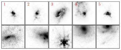
Figure 7: Randomly chosen examples of galaxy images with $\delta>5$ and $\delta_{\mathrm{F356W}}>10$ (see Figure 5). For each of the examples, we show noiseless and noise-added images in the F200W (top rows) and F356W (bottom rows) filters.

3.5 Dependence on physical and photometric parameters

An advantage of calibrating the neural network model with simulations is that we have access to a large number of physical properties of the galaxies. An additional test for our classification scheme is, therefore, to examine how the representation space is correlated with physical quantities as well as with other (more standard) morphological measurements.

3.5.1 Correlation with physical properties

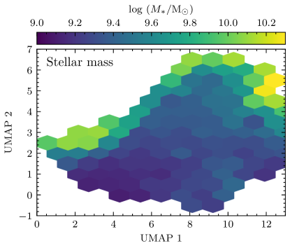
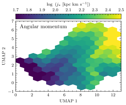
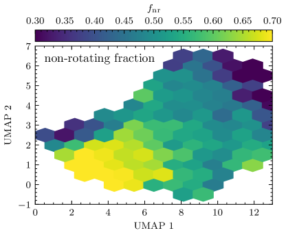
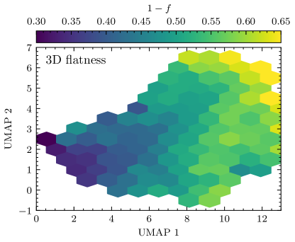
Figure 8: UMAP visualization for all the TNG50 galaxy images in our dataset color-coded by the distribution of several physical properties extracted from the TNG50 simulation. Color code corresponds to the median values in each hexagonal bin in the UMAP plane. From left to right and top to bottom, the different panels show: the logarithm of the total stellar mass ($\log M_{*}\mathrm{[M_{\odot}]}$), the logarithm of the specific angular momentum of the stars ($\log j_{*}\mathrm{[kpc~{}km~{}s^{-1}]}$), the mass fraction in non-rotating stars ($f_{\mathrm{nr}}$), and the galaxy flatness ($1-f$). The scatter maps of these parameters are presented in Appendix A.

In this section, we discuss how some physical properties extracted from the TNG50 simulation correlate with the representation in the UMAP plane. In Figure 8, we show the dependence in the UMAP plane with the total stellar mass ($M_{*}\mathrm{[M_{\odot}]}$), the specific angular momentum of stars ($j_{*}\mathrm{[kpc~{}km~{}s^{-1}]}$), the mass fraction in non-rotating stars ($f_{\mathrm{nr}}$) and the flatness ($1-f$) of the galaxy. The mass fraction in stars that have no net angular momentum around the $z$-axis is defined using the circularity parameter $\epsilon=J_{z}/J(E)$, as in Marinacci et al. (2014), for every star particle. It measures the maximum specific angular momentum possible at the specific binding energy E of the star. The mass fraction in non-rotating stars mass (denoted as $f_{\mathrm{nr}}$) is then defined as the fractional mass of stars with $\epsilon<0$ multiplied by two. The flatness of the galaxy is computed as follows: $f=c/\sqrt{ba}$, where $c<b<a$ denote the principal axes obtained as the eigenvalues of the mass tensor of the stellar mass inside $2r_{*}$. The larger $1-f$ is, the flatter the system is in 3D. Here and throughout the paper we refer to the definitions and measurements of Pillepich et al. (2019). See also section 6 for a more detailed discussion of the 3D shapes of the TNG50 galaxies.

Figure 8 shows remarkable correlations between the position of galaxies in the UMAP and their average physical properties. Overall, galaxies with larger specific angular momentum and a flatter stellar distribution tend to populate the upper-right region of the UMAP. These galaxies are also the most massive ones although the correlation is less clear. Moreover, the galaxies with larger masses not only occupy the upper-right section of the UMAP plane but also extend along the upper edge towards the left corner of the UMAP plane. On the contrary, low-mass galaxies populate predominantly the bottom-left section of the UMAP representation. The left section of the UMAP plane is populated by rounder objects with lower specific angular momentum. It is also interesting to see that the transition between the variation of the physical properties is smooth, translating a continuum of galaxy morphology/structure.

Figure 8 only shows the median values of the physical properties in different regions of the UMAP. In order to quantify how constraining are these correlations, it is also important to measure the scatter of the different properties. This is shown in the appendix A (Figure 20). In most cases, the scatter represents less than $\sim 20\%$ of the dynamical range, indicating that the distributions are overall relatively narrow and, therefore, the correlations with physical properties are informative.

We conclude that the representation space for images —in addition to being robust to observational and instrumental effects— carries information about the kinematics and intrinsic shapes of galaxies.

3.5.2 Connection to standard morphological measurements

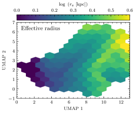
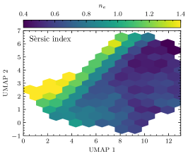
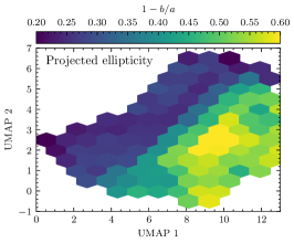
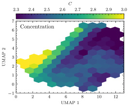
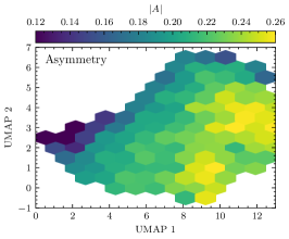
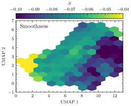
Figure 9: UMAP visualization for all the TNG50 galaxy images in our dataset color-coded by the distribution of several morphological and photometric parameters. Color code corresponds to the median values in each hexagonal bin in the UMAP plane. From left to right and top to bottom, the different panels show: the logarithm of the effective radius ($r_{e}\mathrm{[kpc]}$), in kpc), the Sèrsic index ($n_{e}$), the ellipticity based on Sèrsic fit ($1-b/a$), the concentration ($C$), the asymmetry ($A$) and the smoothness ($C$). The scatter maps of these parameters are presented in Appendix A.

In Figure 9, we show the dependence on several photometric parameters estimated by Costantin et al. (2023) in the F200W filter: the effective radius ($r_{e}$), the Sèrsic index ($n_{e}$), the ellipticity from the Sèrsic fit ($1-b/a$), the concentration parameter ($C$), the asymmetry ($|A|$) and the smoothness ($S$). There is a remarkable correlation between the position in the UMAP plane and $n_{e}$, $C$, $A$, and $S$. Gradually, $n_{e}$, $C$, and $S$ grow from right to left in the UMAP space, while the $A$ does it from left to right. Therefore, galaxy images with smoother, symmetric, and concentrated light distributions are found towards the left section of the UMAP plane. Also important is the correlation with the ellipticity ($1-b/a$), with more elongated galaxies lying on the right (bottom-right) section of the UMAP plane. To illustrate again the spread of these representations, we show in the appendix A (Figure 21) the scatter of the parameters shown in Figure 9.

It is important to notice the existing correlation with the physical effective radius, $r_{e}$, with the largest galaxies populating the right section of the UMAP plane. This correlation with the physical size reflects the known correlation between morphological appearance and physical size (e.g.,van der Wel et al., 2014a).

Based on the previous maps calibrated with the TNG50 simulation, asymmetric, more extended, flatter, and rotationally-supported galaxies tend to populate the right and upper-right sections of the UMAP representation. In more detail, the more to the right in the UMAP plane a galaxy is, the more elongated it appears. Smoother, more compact, rounder, and non-rotating galaxies are located toward the left section of the UMAP representation. Also, less massive galaxies can be found predominantly towards the bottom and bottom-left sections of the UMAP plane. Although not shown, the results presented here are consistent (despite small variations) for the same morphological parameters measured in the F365W filter.

4 Self-supervised learning representation of JWST galaxy images

In this section, we apply the methodology described before to the two datasets of observed galaxies with JWST described in subsection 2.1.

4.1 Representations of CEERS galaxy images

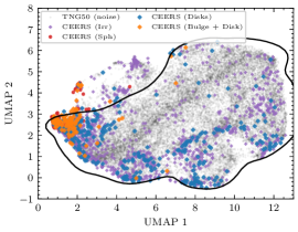
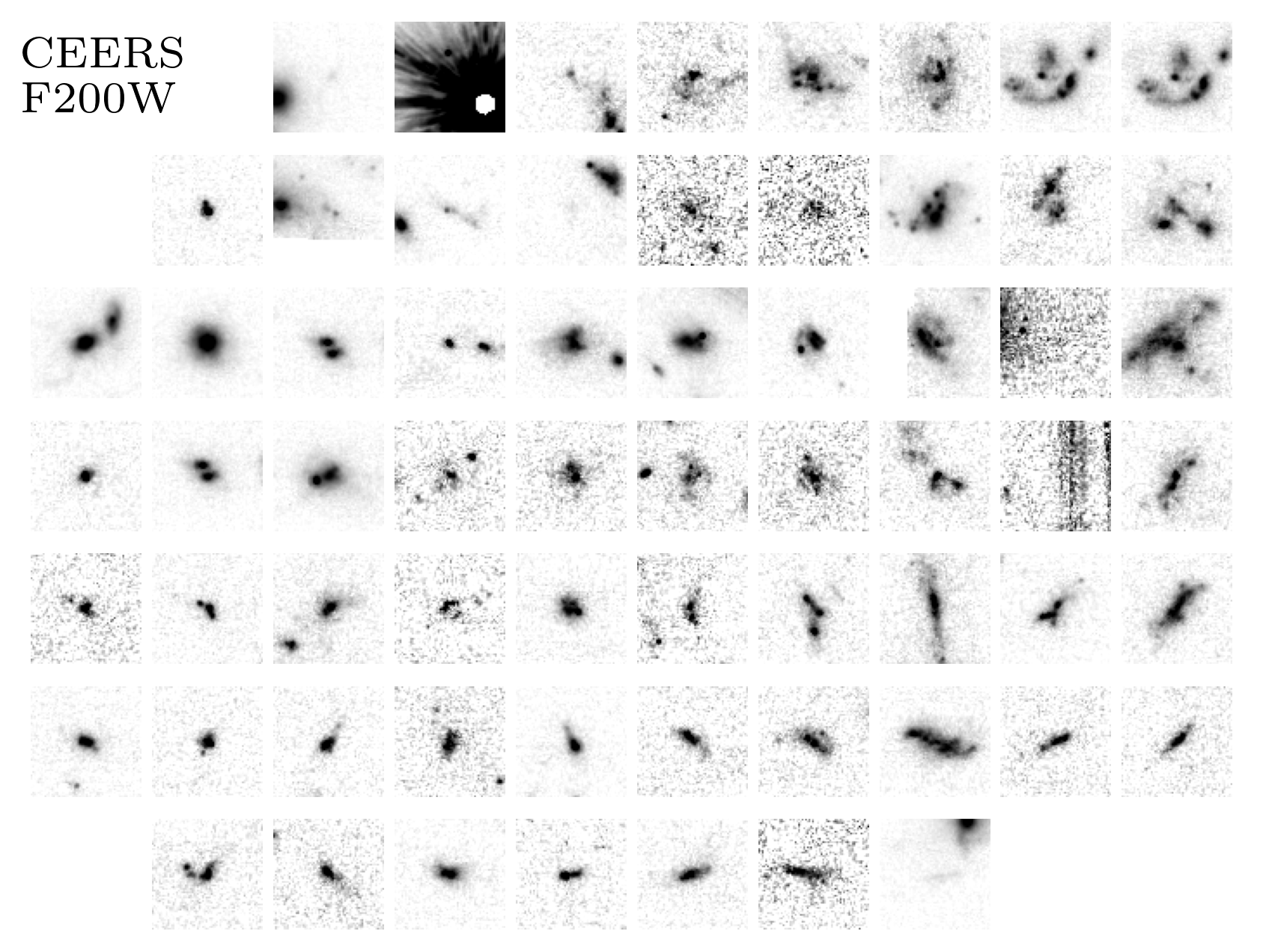
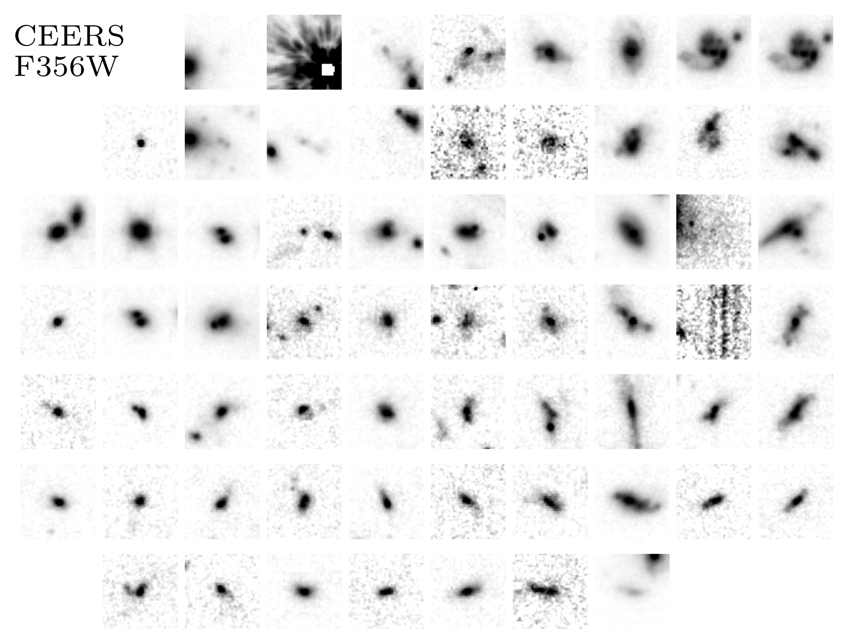
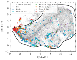
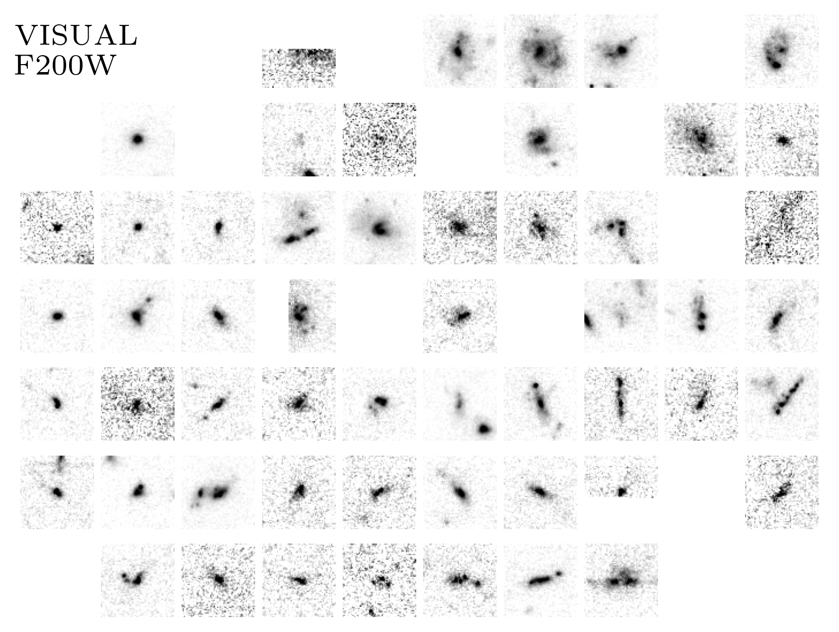
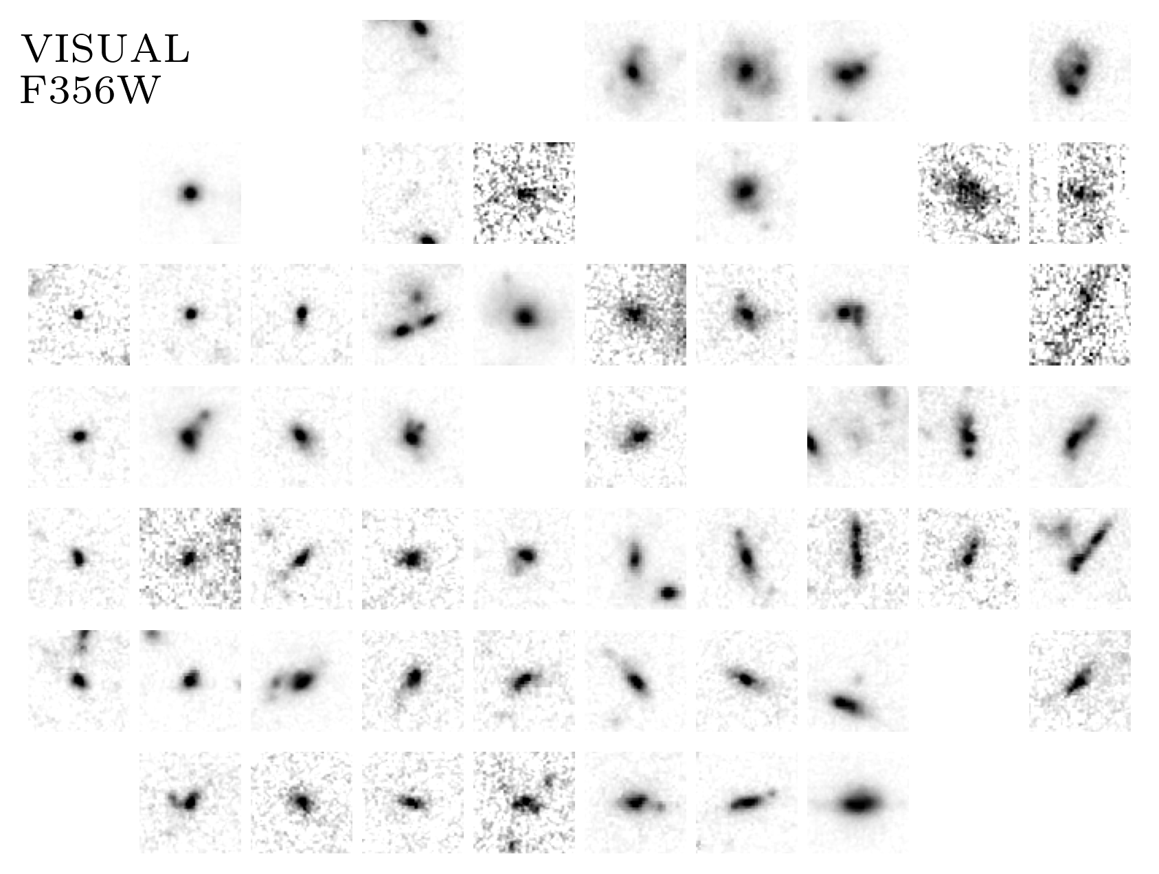
Figure 10: Comparison of distributions of observed and simulated galaxies in the representation space. The top row shows the CEERS mass-complete sample and the bottom row the VISUAL sample. Top left-hand panel: UMAP visualization for the observed CEERS galaxy images selected in mass and redshift (color-coded by the CNN-based morphological classes derived in Huertas-Company et al. 2023b for the F356W filter) overlapped with the representation of noise-added TNG50 galaxy images. Black contour indicates the region that is not affected by extremely bright companions. Top middle panel: randomly chosen observed CEERS galaxy images in the UMAP visualization in the F200W filter. Top right-hand panel: randomly chosen observed CEERS galaxy images in the UMAP visualization in the F356W filter. Bottom left-hand panel: UMAP visualization for the observed VISUAL galaxy images selected in mass and redshift. Points are colored according to the visual classifications into several classes. Black contour indicates the region that is not affected by extremely bright companions. Bottom middle panel: randomly chosen observed VISUAL galaxy images in the UMAP visualization in the F200W filter. Bottom right-hand panel: randomly chosen observed VISUAL galaxy images in the UMAP visualization in the F356W filter.

We feed the 1 664 observed CEERS galaxies to our contrastive model to retrieve their corresponding representations in the 1 024 dimensions space. Then, we normalize the derived features and transform them into a 2D vector using the same UMAP embedding obtained for the features of the TNG50 galaxy images.

In the top row of Figure 10, we show the UMAP representation space for the observed CEERS dataset. Interestingly, observed galaxies tend to populate the complete UMAP plane which indicates that both samples share similar morphological diversity. The UMAP visualization is however a projection of a higher dimension space, which is not appropriate for outlier detection. Even if observed galaxies would not reside in the same manifold as simulated objects, the UMAP representation would tend to show them towards the edges of the plane but not outside. This is the behavior seen for observed CEERS galaxies which tend to be concentrated in the edges of the UMAP cloud (towards the bottom and bottom-left sections) independently of the source redshift. Given that the mass and flux distributions of both datasets are consistent —even though we have not performed a careful one-to-one match between simulations and observations— the differences in the distributions of points of both datasets are likely to originate in intrinsic differences in the morphological properties. Combining the distributions of points in Figure 10 with the information provided by Figure 8 and Figure 9, we conclude that observed CEERS galaxies occupy more frequently than the simulated TNG50 galaxies the regions in the representation space where galaxies are more compact and with less specific angular momentum. We investigate these differences in more detail in section 5.

Also interesting is the presence of galaxy images with signs of interactions, multiple clumps, and gas accretion processes in the upper-right section of the UMAP in Figure 10 (more clear in the F200W filter because of its better spatial resolution compared to the F356W filter). Moreover, galaxy images with double nuclei (or even multiple clumps) closer in projection tend to appear in the bottom-right section of the UMAP plane. These systems are apparently more elongated and, therefore, lay into the region of the UMAP plane where the projected ellipticities are on average larger (as shown in Figure 9), but less flat than the systems located on the upper-right section of the UMAP plane (as shown in Figure 8).

Following subsection 3.4, hereafter, we only include galaxies located within the black contours shown in Figure 10, for which it is unlikely to find bright companions or artifacts that could bias their representations. We find that $\sim 90\%$ ($1\,481$) of the galaxies fulfill this criterion, while the remaining $\sim 10\%$ are excluded from the subsequent analysis. In this dataset and according to the morphologies based on the F356W filter, 121 galaxies ($\sim 8\%$) are classified as Sph, 297 galaxies ($\sim 20\%$) are classified as Disk, 96 galaxies ($\sim 6\%$) are classified as Bulge + Disk and 967 galaxies ($\sim 65\%$) are classified as Irr. If we focus on the morphologies obtained from the F200W filter, the fraction of Irr galaxies raises up to $\sim 82\%$ and the fraction of Disk galaxies decreases down to $\sim 6\%$.

4.2 Representations of VISUAL galaxy images

We also present a comparison of the representation obtained after applying our contrastive model to the VISUAL dataset for which visual morphological classifications are provided (Kartaltepe et al., 2023). After selecting those galaxies with $M_{*}\geq 10^{9}\mathrm{M_{\odot}}$, $3<z<6$, and reliable visual classifications we end up with a dataset of 545 galaxies. To avoid including in the analysis galaxy images with contaminants or artifacts, hereafter, we only consider those galaxies located within the black contours shown in Figure 10. In this case, we are confident about the representations obtained for $\sim 90\%$ (483) of the galaxy images, for which we find: 118 ($\sim 24\%$) Disk galaxies, 102 ($\sim 21\%$) Disk+Irr galaxies, 24 ($\sim 5\%$) Disk+Sph+Irr galaxies, 56 ($\sim 11\%$) Disk+Sph galaxies, 71 ($\sim 14\%$) Sph galaxies, 22 ($\sim 4\%$) Sph+Irr galaxies, 81 ($\sim 16\%$) Irr galaxies, and only 2 and 7 as point sources and unclassifiable galaxies, respectively.

In the bottom row of Figure 10, we show the representation of the galaxy in the VISUAL dataset in the UMAP plane for the various morphological groups based on the provided visual classifications. Although the mass and redshift selection of the galaxies is based on different estimators (JWST photometry for the CEERS dataset and CANDELS photometry for the VISUAL dataset), the distribution of the representations in the UMAP plane for the VISUAL galaxies is similar to the CEERS representations (i.e., a significant fraction of galaxies occupy the bottom and bottom-left section of the UMAP plane). The figure reveals some expected correlations with the traditional visual morphology. It is reassuring that Disk+Sph and Sph groups from the VISUAL catalog populate the left corner of the UMAP plane, where compact, non-rotating galaxies with low angular momentum (according to TNG50 properties) are expected to be. However, we notice that galaxies classified as Disk, Irr and/or Disk+Irr in VISUAL are distributed throughout the plane even towards the left section of the UMAP, very close to where spheroids lie. As shown in Figure 8 and Figure 9, the left region of the UMAP where, according to VISUAL, disk-like morphologies are located corresponds to galaxies in TNG50 with physical and photometric properties typically shared by spheroidal systems, such as low specific angular momentum, large mass fractions in a non-rotating component, low flatness, and larger Sèrsic indexes. This raises interesting questions about the true nature of these disks that we discuss in section 6.

5 A comparison between simulated and observed self-supervised morphologies

In this section, we examine in more detail the differences found in previous sections between the simulated TNG50 and the observed JWST galaxy images.

5.1 Distribution of self-supervised representations

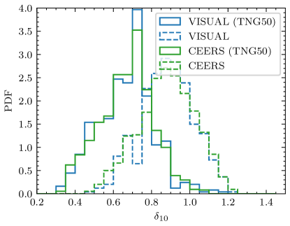
Figure 11: Probability density functions of the distances to the 10th closest neighbor in the 1 024 dimensions of the representation space, denoted as $\delta_{10}$. Solid histograms correspond to the distance to the 10th closest neighbor in TNG50 of the closest TNG50 neighbor of each galaxy in the VISUAL (in blue) and the CEERS (in green) datasets. Dashed histograms correspond to the distance to the 10th closest neighbor in TNG50 of each galaxy in the VISUAL (in blue) and the CEERS (in green) datasets.

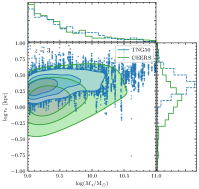
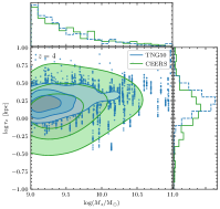
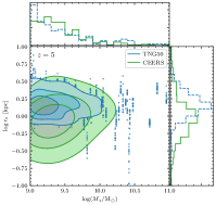
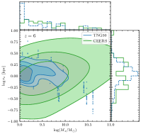
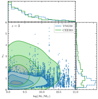
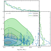
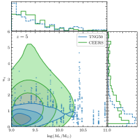
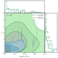
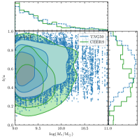
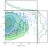
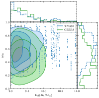
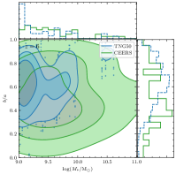
Figure 12: Distribution of the logarithm of the effective radius ($\log r_{e}$ in kpc, top row), the Sèrsic index ($n_{e}$, middle row), and the axis ratio ($b/a$, bottom row) as a function of the logarithm of the stellar mass ($\log M_{*}$) for the TNG50 (in blue) and the CEERS (in green) datasets. From left to right, the panels show the distributions at $z=3,4,5,6$ for the TNG50 dataset. For the CEERS dataset, galaxies are included in the closest redshift value. Contour levels enclose $25\%$, $50\%$, and $75\%$ of the data. Blue points correspond to galaxies outside the $75\%$ contour for the TNG50 dataset. Blue dashed and green solid histograms in the horizontal and vertical axes show the PDF of the TNG50 and CEERS datasets, respectively. The photometric parameters shown are measured in the F200W filter.

The representations of the simulated TNG50 and the observed CEERS galaxy images inferred by our contrastive model seem to be distributed differently (subsection 4.1 and subsection 4.2). Observed CEERS galaxies tend to concentrate in the left and bottom-left sections of the UMAP plane, while simulated TNG50 galaxies expand over the whole UMAP range with similar number densities. As previously mentioned, the UMAP representation is not well suited for the detection of outliers. Therefore, even if observed galaxies seem to (overall) lie in the same region as simulated ones, they can still live in different manifolds in the higher dimensionality representation space.

To further quantify this distribution shift, we first derive the distance —in the 1 024 dimensionality space— to the 10th closest TNG50 neighbor for each galaxy in the VISUAL and CEERS datasets (denoted as $\delta_{10}$). In order to have a fair reference distribution, secondly, for each observed galaxy we find the closest simulated TNG50 neighbor in the representation space and compute the distance to its 10th closest TNG50 neighbor (also denoted as $\delta_{10}$). In other words, the former corresponds to the distance between the observed galaxy and its 10th closest TNG50 neighbor, while the latter corresponds to the distance to the 10th closest TNG50 neighbor of the closest TNG50 galaxy to each observed galaxy. If both datasets —observed and simulated— are distributed likewise in the same manifold the distribution of distances should be similar. If, on the contrary, observed galaxies occupy differently the parameter space, their representations should be disconnected and, therefore, we should measure larger values of $\delta_{10}$. The distributions of $\delta_{10}$ are shown in Figure 11. It can be clearly seen that the distributions for observed galaxies are shifted towards larger values compared to the reference distribution. This indicates that a significant fraction of observed galaxies are located in regions of the UMAP representation space with lower number densities (i.e., along the edges, not in the central regions) than the average of the TNG50 dataset. This separation could be interpreted as an additional indication that the representations obtained for the TNG50 and the JWST observations do not exactly live in the same manifold. Nevertheless, we find a small fraction of simulated TNG50 galaxies with values of $\delta_{10}\gtrsim 0.9$, meaning that the separation for the most extreme cases is also present for some galaxies in the TNG50 simulation.

To better understand these measured discrepancies, we quantify the differences between observed and simulated galaxies in terms of more standard morphological properties in Figure 12. We show the distributions of observed and simulated galaxies in the $\log M_{*}-\log r_{e}$, $\log M_{*}-\log n_{e}$, and $\log M_{*}-b/a$ planes in four redshift bins. To divide in redshift, for the simulated dataset, we take all galaxies in a given snapshot, while, for the observations, we include all galaxies that are associated with the closest snapshot based on their photometric redshifts. It should be kept in mind that this figure (as the previous ones) does not include all TNG50 galaxies, but those for which the JWST mocks are available for a field-of-view larger than $64\times 64$ pixels (see subsection 2.2 and Figure 2 for more details). Given the small number of galaxies removed, we do not expect the distributions to change significantly though.

It is manifest, firstly, that the TNG50 simulated galaxies overlap with CEERS observed ones in the parameter space of Figure 12. This is per se, again, a non-negligible confirmation of the zeroth-order good functioning of the underlying TNG50 model. However, it is also apparent, differently than what could be deduced from the representation space distributions, that the TNG50 galaxies studied here actually exhibit less galaxy-to-galaxy variation in sizes, Sèrsic indices, and shapes than CEERS observed galaxies, at fixed stellar mass and redshift. Furthermore, the TNG50 simulation predicts galaxies with larger sizes (at $z=3-4$, but not $z=5-6$), with smaller values of $n_{e}$ (at all $z=3-6$) and that are rounder in projection (more so the higher the redshift) than what is measured in the observed CEERS galaxies. These differences at least partly explain the different distributions in the representation space of contrastive learning and also go in the expected direction of observed galaxies mainly populating the left and bottom-left corner of the UMAP.

These reported differences could originate from a resolution-induced effect (see e.g., Zanisi et al., 2021) or could be an indication of more fundamental physical differences. Resolution is certainly an important concern since galaxies at these redshifts are generally small. We recall that although the TNG50 has a softening length for stellar particles of $\sim 300~{}\mathrm{pc}$, it does not mean that galaxies’ stellar disks cannot be thinner than that softening length. The interplay of the various numerical resolution choices (such as gravitational softening of the different matter components, hydrodynamical smoothing length of the gas out of which stars form, mass resolution, etc.) manifests itself in very complex manners in the final structures of the simulated galaxies (see e.g. Section 2.3 of Pillepich et al., 2019 or Section 2.4 of Pillepich et al., 2023). As shown in Pillepich et al. (2019) (Figures 4 and B2), the half-light or half-mass heights of TNG50 galaxies can be smaller than $\sim 300~{}\mathrm{pc}$ depending on mass and redshift. Similarly, the stellar minor-to-major axis ratios of the stellar mass distributions of TNG50 galaxies can be smaller than $b/a\sim 0.3$, as shown in e.g. Figure 8 (top panels) of Pillepich et al. (2019), again depending on mass and redshift. In fact, in Figure 12, it can be clearly seen how the axis ratios extend down to $b/a\sim 0.2$ (mainly at $z=3-4$). Moreover, as shown in Appendix B2 of Pillepich et al. (2019), TNG50 disk heights can be considered converged to better than $20--40\%$ across all studied masses and redshifts, when compared to the same galaxies simulated at worse numerical resolution.

We note as well that the stellar masses reported for the TNG50 simulation correspond to the 3D stellar mass, while those obtained for the CEERS dataset are based on the SED fitting to the JWST photometry. Also, the Sèrsic parameters for the TNG50 and the CEERS galaxies are derived using different methodologies: for the TNG50, the morphological parameters are obtained with statmorph (as described in Costantin et al. 2023); while for the CEERS dataset, they are derived with galfit.

More in-depth comparisons of simulated and observed data —likely beyond images— are required to reach a final conclusion.

5.2 Self-supervised clustering in TNG50 and CEERS

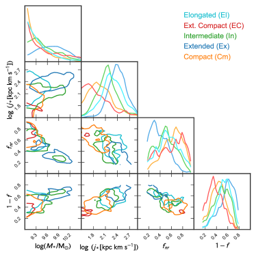
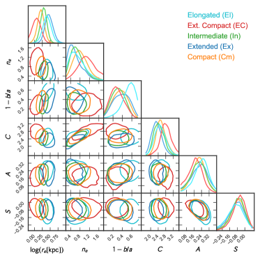
Figure 13: Triangle plot with physical properties extracted from the TNG50 simulation (left-hand panel) and morphological (right-hand panel) properties of the morphological clusters shown in the left-hand panel in Figure 14. For clarity, only the $68\%$ contour levels are shown.

As an additional way to quantify the differences between TNG50 galaxies and observed CEERS galaxies, we compare the abundances of TNG50 and CEERS galaxies retrieved from the separation into different classes using a clustering technique.

In particular, we apply the $k-$means algorithm to cluster data in the representation space by trying to separate samples in $k$ groups of equal variance, minimizing a criterion known as the inertia or within-cluster sum-of-squares (WCSS). We find $k=5$ as the optimal number of clusters based on the Elbow curve. The elbow method is a graphical representation of finding the optimal $k$ in a $k-$means clustering. It works by finding WCSS (Within-Cluster Sum of Square), i.e. the sum of the square distance between points in a cluster and the cluster centroid. This result is also confirmed using an alternative method based on the Silhouette score. We implement the Elbow and Silhouette methods using the Yellowbrick package in python (see Bengfort et al. 2018, for more details).

We label the different clusters according to the properties (photometric and morphological) of the galaxies belonging to each of them. In Figure 13, we show the properties (and correlations between them) of the different classes. Therefore, we define the following classes: Extremely Compact (EC), Compact (C), Intermediate (In), Elongated (El) and Extended (EX). It is clear how EC and C galaxies show low mass, low angular momentum, large fractions of non-rotating stars, and low flatness. They are also smaller in size with larger Sèrsic index values, rounder in projection, and more compact than the rest of the classes. As going from the In class to the El and EX classes, the masses and sizes of the galaxies progressively increase along with the angular momentum of the stars and the flatness. These classes also exhibit smaller Sèrsic indexes and are less concentrated and more asymmetric than the compact classes. Also interesting is the separation in the projected ellipticity of the El class, showing extremely large values of the $1-b/a$ compared to the rest of the classes.

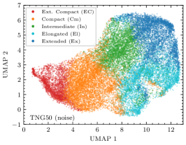
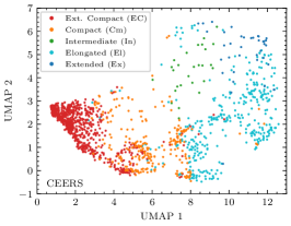
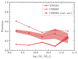
Figure 14: Left-hand panel: UMAP visualization of noise-added TNG50 galaxy images color-coded by classes according to the $k$-means method for five clusters. Morphological classes are labeled as: Extremely Compact (EC, in red), Compact (C, in orange), Intermediate (In, in green), Elongated (El, in cyan) and Extended (EX, in blue). Middle panel: same as the left-hand panel but for the CEERS galaxy images. Right-hand panel: fractions Extremely Compact (EC) galaxies (i.e., those belonging to the EC cluster in red) in TNG50 (solid lines), CEERS (dashed lines) and CEERS with $\log r_{e}\mathrm{[kpc]}>0$ (dotted lines) in 5 logarithmic mass bins of width 0.5 dex in the range $9<=\log(M/\mathrm{M_{\odot}})<=11.5$. The shaded regions correspond to the fraction errors considering Poisson errors in the number of selected galaxies and the total number of galaxies in each mass bin. Note that for clarity we do not show the shaded region for the CEERS dataset without applying any cut in size.

For the simulated TNG50 galaxies, we find: $\sim 12\%$ of EC galaxies, $\sim 26\%$ of Cm galaxies, $\sim 19\%$ of In galaxies, $\sim 22\%$ of El galaxies and $\sim 20\%$ of EX galaxies. While for the observed CEERS dataset, we find $\sim 55\%$ of EC galaxies, $\sim 17\%$ of Cm galaxies, $\sim 2\%$ of In galaxies, $\sim 25\%$ of El galaxies and $\sim 2\%$ of EX galaxies. Therefore, and also clear from Figure 14, there is a systematic lack of observed CEERS galaxies in the rest of the classes beyond the EC class, with the exception of the El class, for which the fractions of observed galaxies are slightly larger than for the simulated ones. In particular, the fractions of observed CEERS galaxies in the In and EX classes are significantly smaller than those for the simulated TNG50 ones.

In Figure 14, we show the UMAP visualization color-coded by the five classes for the simulated TNG50 and the observed CEERS datasets. Note that galaxies with artifacts or bright companions are not included in the derivation of the different class fractions. Given the division and the correlations shown in Figure 8 and Figure 9, we denote the galaxies located in the left section of the UMAP that belong to the cluster in red as Extremely Compact (EC) galaxies, while the remaining galaxies (i.e., those not assigned to the red EC cluster) are considered as non-compact (NC) galaxies. We find that on average $\sim 12\%$ of the TNG50 galaxies belong to the EC class. For the CEERS dataset, we find that $\sim 55\%$ of the CEERS galaxies belong to the EC class. In order to mitigate the possible effects of resolution in the simulation, we additionally impose a minimum size threshold for CEERS galaxies and only include CEERS galaxies with $r_{e}>1\mathrm{kpc}$, measured in the F200W filter. This excludes the low-radius tail of $5\%$ of the TGN50 galaxies and $\sim 50\%$ of the CEERS dataset (mainly spheroids since they are typically smaller in size). We find that the fraction of galaxies in the EC class for the CEERS dataset is reduced to $\sim 37\%$, but the discrepancy between observations and simulations is still significant.

Our results tend to confirm that the TNG50 model systematically under-predicts the abundance of compact galaxies from a purely data-driven perspective, similar to the findings of e.g. Flores-Freitas et al. (2022). The effect does not seem a pure consequence of resolution.

6 A comparison between self-supervised and supervised morphologies

We now compare in more detail the CNN-based and visual classifications for the CEERS and VISUAL datasets with the self-supervised classifications —which have been shown to correlate with physical properties— and speculate about the abundance of disks at $z>3$. As shown in section 4.1, visually classified disks are spread all over the representation space which suggests that, according to the self-supervised representations, they represent a heterogeneous group of galaxies with different physical properties.

6.1 Self-supervised clustering vs. morphological classifications

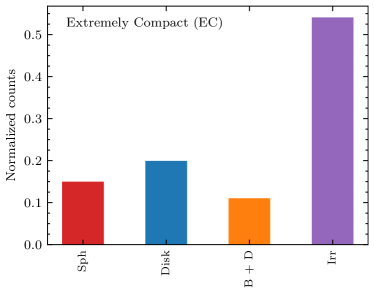
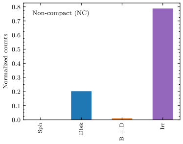
Figure 15: Comparison of the classification into Extremely Compact (EC, left-hand panel) and non-compact (NC, right-hand panel) galaxies in the CEERS dataset and the CNN-based classifications derived by Huertas-Company et al. (2023b). Histograms are color-coded according to the CNN-based morphological classes into: Sph in red, Disk in blue, Bulge + Disk (B+D) in orange, and Disturbed (Irr) in purple.

In Figures  15 and 16, we show a comparison between the CNN-based and visual classifications with the two broad contrastive learning clusters containing Extremely Compact (EC) and Non Compact (NC) galaxies, respectively.

The figures show that, for both the CNN and visual classifications, almost all galaxies classified as spheroids or with a bulge component belong to the EC cluster. This is expected as the EC cluster lies in a region of the representation space dominated by round and compact galaxies. However, the trend for disks and irregular galaxies is not so clear. The figures show that both the EC and NC clusters contain a large fraction of disks and irregular galaxies, which reflect the fact that disks and irregulars are distributed over all the representation space. In fact, we measure that each cluster contains roughly $\sim 50\%$ of the Disk and Irr galaxies for both the CEERS and the VISUAL datasets. This discrepancy between the self-supervised and the traditional classes is somehow surprising and suggests that the population of visually classified disks and irregulars present a large spread of morphological properties that the contrastive learning representation is capturing. We quantify this further in the following. We emphasize that this discrepancy between supervised and self-supervised classifications is independent of the degree of agreement between simulations and observations discussed in section 5.

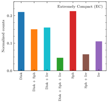
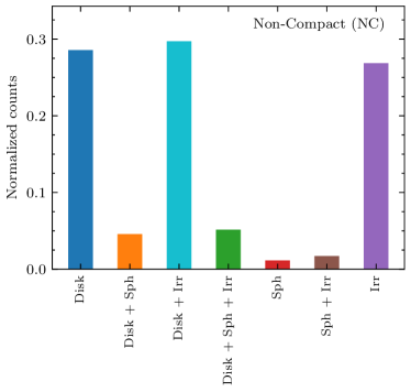
Figure 16: Comparison of the classification into Extremely Compact (EC, left-hand panel) and non-compact (NC, right-hand panel) galaxies in the VISUAL dataset and the visual classifications derived by Kartaltepe et al. (2023). Histograms are color-coded according to the visual morphologies as in Figure 10.

6.2 Two populations of visually classified disks?

Based on the positions of the visual disks in the contrastive learning representation space, we identify two different populations of visually classified disks which we call EC Disks and NC disks, for Extremely Compact and Non Compact disks, respectively.

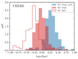
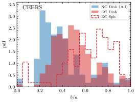
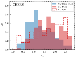
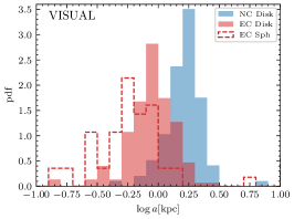
Figure 17: Morphological and photometric properties of the two populations of disk-like galaxies in the CEERS (top panels) and the VISUAL (bottom panels) datasets. From left to right, the different panels show the probability distribution function of the size of the galaxy ($\log a\mathrm{[kpc]}$), the projected ellipticity ($b/a$), and the Sèrsic index ($n_{e}$), respectively. The different histograms correspond to EC Disk candidates (red shaded histograms), NC Disk candidates (blue shaded histograms), and EC Sph candidates (red dashed histograms). For the CEERS dataset, we consider as disk candidates those classified as Disk and Bulge+Disk, while for the VISUAL dataset, we consider as disk candidates the four classes of visually classified disks (Disk, Disk + Sph, Disk + Irr, and Disk + Sph + Irr). All quantities are derived from the Sèrsic fits in the F356W filter.

In order to get more insights about why the self-supervised learning algorithm tends to locate them in different clusters, we then examine the properties of the EC Disks and NC Disks using parametric morphologies obtained via Sèrsic fitting in the F356W filter (see section 2 for more details). In Figure 17, we show the distributions of axis-ratios ($b/a$), semi-major axes ($a$), and Sèrsic indices ($n_{e}$) for the two disk classes, and for the CEERS and VISUAL datasets. We also show, for reference, the same distributions for galaxies visually classified as spheroids.

The figure clearly shows different distributions. As expected, EC Disks have smaller effective radii. The NC Disks exhibit a distribution of $\log a$ that peaks at $\log a\sim 0.25$, while for the EC Disks it peaks at smaller values of $\log a\sim-0.10$. The distribution of $n_{e}$ is also different and reflects that EC Disk are more concentrated. For NC Disks, it peaks at $n_{e}\lesssim 1.2$, characteristic of an exponential profile. However, for EC Disks, the distribution is skewed towards larger values of the Sèrsic index, although smaller than for spheroids. Regarding the $b/a$ distribution, the NC Disks tend to be more elongated, and, as expected, spheroids are rounder on average. The EC Disk candidates are in between, with a peak at $b/a\sim 0.5$.

In view of these differences and the correlations between structural properties and the positions in the representation space highlighted in previous sections, it is expected that the NC and EC Disks fall in different regions of the parameter space, even if they share the same visual classification. It also makes sense that these EC Disks are generally classified as disks by expert classifiers given the proposed classification scheme, in the sense that they do not show strong signs of irregularities and are more elongated and less concentrated than pure spheroids. Therefore, by default, they end up in the disk class. In Appendix B, we show examples of several NC Disks and EC Disks candidates (including some cases with $b/a<0.3$) along with various EC Sph candidates for comparison.

The difference between the completely supervised and self-supervised classifications illustrates how a purely data-driven approach can offer an alternative description of the information content of the data. It is also important to highlight that the difference between the two types of classifications is not only driven by differences in size. The distributions of $\log a$ plotted in Figure 17 overlap significantly. In addition, if we only include in the analysis galaxies with $r_{e}>1\mathrm{kpc}$, there is still a significant fraction ($\sim 40\%$) of visually classified disks in the EC cluster.

An interesting question, therefore, is whether NC and EC Disks are all true disks —if by disk we understand a flat system predominantly supported by the rotation of the gas and stars— as this has important implications on the frequency of disk formation at these very early cosmic epochs. It is certainly impossible to unambiguously answer this question with the data at hand. However, we can speculate based on the information inferred from the TNG50 simulation. As shown in the previous subsections, there is a strong correlation between the contrastive learning representations and the stellar specific angular momentum. Interestingly, the location of EC Disks is predominately populated by low angular momentum galaxies, which would suggest that these systems are preferentially velocity dispersion supported.

As an additional attempt to shed some light on the physical properties of EC and NC Disks, we explore in more detail how the contrastive learning representation space distributes galaxies with different 3D stellar structures. We characterize the shape of galaxies in the TNG50 sample as done and studied in Pillepich et al. (2019), i.e., with an ellipsoid with three semi-axes $c<b<a$ and use the axial ratios $q=b/a$ (intermediate-to-major) and $s=c/a$ (minor-to major) to define three main 3D shape classes: oblate, spheroid and prolate following the definitions of van der Wel et al. (2014b) and Zhang et al. (2019). The axial ratios are derived after diagonalizing the stellar mass tensor in an iterative way while keeping the major axis length fixed to $2r_{*}$. We consider oblate or disk galaxies those with $a\sim b>c$, elongated or prolate objects those with $a>b\sim c$, and spheroidal systems those with similar values for the three semi-axes. Note that, by definition, the 20 projections of the TNG50 galaxies have the same 3D shape. At these redshifts, we find that $\sim 67\%$ of the galaxies in the simulation have a spheroidal shape according to this definition. Only $18\%$ and $15\%$ of the galaxies have oblate and prolate shapes, respectively. The fact that at high redshift and low stellar masses, galaxies tend to present a more prolate structure has been found both in observations (van der Wel et al., 2014b; Zhang et al., 2019) and simulations (Tomassetti et al., 2016; Pillepich et al., 2019).

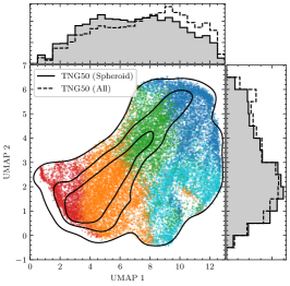
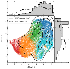
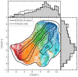
Figure 18: Location in the UMAP plane of TNG50 galaxies according to the 3D shape inferred from the stellar particles: spheroid (left-hand panel), oblate (middle panel), and prolate (right-hand panel). Points are color-coded according to the morphological classes described in subsection 5.2. The contour levels indicate the $25\%$, $50\%$, and $95\%$ probabilities. Unfilled black dashed and filled solid histograms in the horizontal and vertical axes show the PDF of the whole dataset and the shape-selected galaxies of the TNG50 dataset, respectively. Morphologically disk (i.e., oblate) galaxies tend to populate the right and upper-right regions of the UMAP plane, while it is unlikely to find them in the left section of the UMAP plane.

We show in Figure 18 the distribution of the mock images of oblate galaxies in the UMAP projection of the representation space obtained with contrastive learning. For clarity, we do not show the distributions of prolate and spheroidal galaxies. Interestingly, the bottom right corner, where the EC Disks lie, does not contain almost any oblate system. The result would suggest that EC Disks are very unlikely to be true disks (i.e. flat rotating systems) even if they appear as elongated in the images. Despite the small number of TNG50 galaxies with $b/a\lesssim 0.4$, we find that EC TNG50 galaxies with $b/a\lesssim 0.4$ are more likely to be prolate than spheroid in shape, as shown in Figure 19.

However, a big caveat is that the previous statements rely of course on the calibration with the TNG50 simulation, which as shown in the previous sections, does not properly reproduce the observed morphological diversity. Therefore, no firm conclusion can be established without more observations and comparisons with other state-of-the-art simulations. As a matter of fact, an alternative explanation for the different representations of EC Disks and NC Disks could be that the simulation cannot generate compact disks because of resolution issues, as already acknowledged. This would imply that the location of the EC Disks in the representation space cannot be interpreted in terms of physical properties, as these systems simply do not exist in the simulation. We expect the fine-tuning of the model presented in subsection 3.1 should mitigate this effect, but cannot be guaranteed. Nevertheless, our data-driven analysis suggests that robustly establishing the fraction of disk galaxies at $z>3$ remains an open issue.

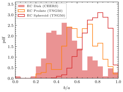
Figure 19: Distributions of projected ellipticity ($b/a$) for EC Disk candidates in CEERS (red shaded histogram), and EC prolate and spheroid TNG50 candidates (orange and red empty histograms, respectively). Elongated galaxies in projection (i.e., $b/a\lesssim 0.4$) are compatible with being prolate in shape according to the TNG50 EC prolate candidates.

7 Summary and Conclusions

This work presents a novel data-driven method based on contrastive learning to infer the morphological properties of galaxies observed with JWST. The method is calibrated on mock JWST galaxy images extracted from the TNG50 cosmological simulation that, thanks to its large number of qualitatively realistic galaxies, allows us to produce a morphological description —without any assumption on galaxy classes— robust to background noise, signal-to-noise, color, and orientation. In addition, we show that the obtained representations of galaxies based on their images correlate well with some other physical properties inferred from the simulation (such as the specific angular momentum of stars, $j_{*}$, and the intrinsic 3D shape) along with some measured photometric and structural properties (such as Sèrsic index and the projected ellipticity).

We have applied the method to JWST images from the CEERS survey in the F200W and F356W bands of: 1) a mass-complete sample ($M_{*}\geq 10^{9}\mathrm{M_{\odot}}$) of galaxies at $3<z<6$ in the CEERS survey for which CNN-based classifications are available; and 2) a mass- and a redshift-selected sample of CEERS galaxies at $3<z<6$ with $M_{*}\geq 10^{9}\mathrm{M_{\odot}}$ for which visual morphological classifications are available.

Our main results are:

• Simulated galaxies from the TNG50 cosmological simulation seem to cover well the observed morphological diversity at $z>3$. However, the morphological distributions of CEERS and simulated galaxies are measured to be different. When compared at the pixel level, simulated and observed galaxies seem to populate in different proportions in the different regions of the TNG50-trained manifolds. We show that these differences can be at least partly explained because observed galaxies can be more compact and more elongated than simulated ones. In fact, the galaxy-to-galaxy variation in sizes, Sèrsic indices, and shapes at fixed stellar mass and redshift are larger in the observed CEERS population than in TNG50 simulated ones. These differences might be partly explained by the limited resolution of the TNG simulation, but not completely since the discrepancies are not erased when only large galaxies are considered.

• Our morphological description also suggests that CNN-based and visually classified disks comprise two different populations: one made of extremely compact (EC) Disks and another of non-compact (NC) Disks. Half of the galaxies that are classified as disks are indeed located in the representation space very close to compact spheroids and, therefore, are more consistent with not being pure disk-like galaxies (i.e., having a prolate or spheroidal stellar structure). Although some of these conclusions might be affected by the calibration with the TNG50 model, our study suggests that some EC Disk candidates can be misclassified as disks, as they appear (on average) more elongated in the images than EC Sph candidates. The coexistence of prolate and oblate systems at high redshift is in qualitative agreement with the predictions of other models (e.g. zoom-in simulations) which also found that low-mass galaxies at high-$z$ tend to present a prolate shape (Ceverino et al., 2015; Tomassetti et al., 2016). More in-depth follow-up of these two populations of galaxies, possibly with spectroscopy and additional comparisons with other simulations, is required to further constrain their true nature.

Appendix A Scatter of physical and photometric parameters in the UMAP visualization

In Figure 20 and Figure 21, we show the variability in the physical and photometric parameters, respectively, in the UMAP visualization shown in Figure 9 in subsection 3.5. The scatter is quantified as a normalized median absolute deviation, denoted here as NMAD. The median absolute deviation (MAD), defined as $\mathrm{MAD(y)}=median(|y-median(y)|)$, is a robust measure of the variability of a univariate sample of quantitative data. The MAD is less affected by outliers and non-gaussianity than the typical variance and standard deviation. To facilitate the comparison between different variables, we normalized the MAD by the dynamical range of the data, defined as the percentile range containing $98\%$ of the data. The resulting normalized MAD, denoted as NMAD, is an indicator of the variability of the data that, in this case, shows how informative the correlation with the different parameters shown in Figure 8 and Figure 9 are. Values of NMAD $\lesssim 0.2$ are indicative of a low variability of the data.

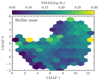
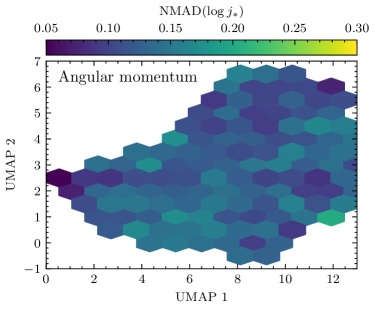
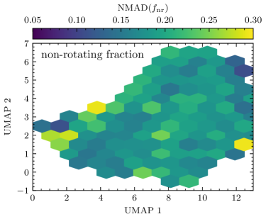
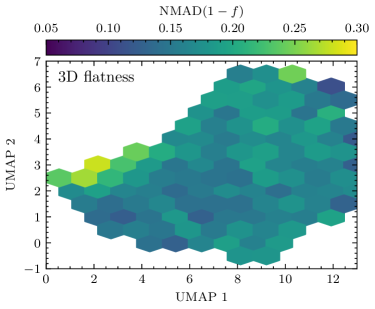
Figure 20: UMAP visualization for all the TNG50 galaxy images in our dataset color-coded by the distribution of several physical properties extracted from the TNG50 simulation. From left to right and top to bottom, the different panels show the UMAP plane color-coded by the NMAD of: the logarithm of the total stellar mass ($\log M_{*}\mathrm{[M_{\odot}]}$), the logarithm of the specific angular momentum of the stars ($\log j_{*}\mathrm{[kpc~{}km~{}s^{-1}]}$), the mass fraction in non-rotating stars ($f_{\mathrm{nr}}$) and the galaxy flatness ($1-f$).

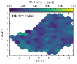
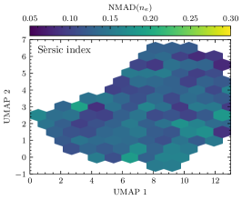
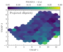
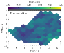
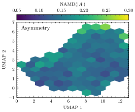
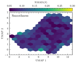
Figure 21: UMAP visualization for all the TNG50 galaxy images in our dataset color-coded by the distribution of several morphological and photometric parameters. From left to right and top to bottom, the different panels show the UMAP plane color-coded by the NMAD of: the logarithm of the effective radius ($r_{e}\mathrm{[kpc]}$), the Sèrsic index ($n_{e}$), the ellipticity based on Sèrsic fit ($1-b/a$), the concentration ($C$), the asymmetry ($A$) and the smoothness ($S$).

Appendix B Examples of observed JWST galaxy images

In Figure 22, we show examples of galaxies in the CEERS dataset that are classified into EC and NC, according to the criterion described in subsection 6.1. For comparison, we show examples of Disk and Sph galaxies following the CNN-based morphological classification presented in (Huertas-Company et al., 2023b). It is clear the differences between the NC Disks and the EC Disks, with more extended and elongated (in projection) light distributions for the NC Disks candidates than for the EC Disks candidates. We also include examples of NC Disks and EC Disks candidates that contribute to the low end of the $b/a$ distribution in Figure 17. In fact, all these examples have values of $b/a<0.3$. For the NC Disks candidates with $b/a<0.3$, they show in almost all the examples signs of multiple clumps and/or in interaction with the central galaxy. For several cases of the EC Disks candidates with $b/a<0.3$, there are also signs of multiple clumps that could lead to an underestimation of the true $b/a$ values.

Moreover, it is difficult to distinguish between some EC Disks and EC Sph candidates, as they exhibit compact and round light distributions, although the EC Disk galaxies appear slightly more elongated (on average) than the EC Sph ones.

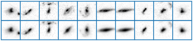
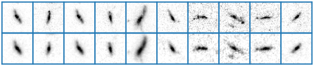
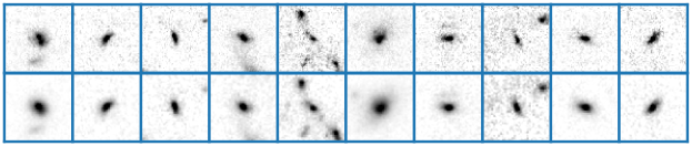
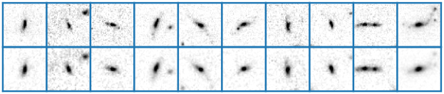
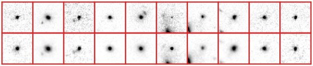
Figure 22: Examples of galaxy images in the CEERS dataset considered as: NC Disks (first row), NC Disks with $b/a<0.3$ (second row), EC Disks (third row), EC Disks with $b/a<0.3$ (fourth row), and EC Sph (fifth row) candidates. Images are framed in color according to the visual classification: blue for Disk and red for Sph candidates. Each galaxy image is shown in the two F200W (top row) and the F356W (bottom row) filters.

References

- Abraham et al. (1996) Abraham, R. G., van den Bergh, S., Glazebrook, K., et al. 1996, ApJS, 107, 1, doi: 10.1086/192352
- Bagley et al. (2023) Bagley, M. B., Finkelstein, S. L., Koekemoer, A. M., et al. 2023, ApJ, 946, L12, doi: 10.3847/2041-8213/acbb08
- Barro et al. (2017) Barro, G., Faber, S. M., Koo, D. C., et al. 2017, ApJ, 840, 47, doi: 10.3847/1538-4357/aa6b05
- Bengfort et al. (2018) Bengfort, B., Danielsen, N., Bilbro, R., et al. 2018, Yellowbrick v0.6, 0.6, Zenodo, Zenodo, doi: 10.5281/zenodo.1206264
- Bournaud et al. (2014) Bournaud, F., Perret, V., Renaud, F., et al. 2014, ApJ, 780, 57, doi: 10.1088/0004-637X/780/1/57
- Buitrago et al. (2014) Buitrago, F., Conselice, C. J., Epinat, B., et al. 2014, MNRAS, 439, 1494, doi: 10.1093/mnras/stu034
- Buitrago et al. (2013) Buitrago, F., Trujillo, I., Conselice, C. J., & Häußler, B. 2013, MNRAS, 428, 1460, doi: 10.1093/mnras/sts124
- Ceverino et al. (2010) Ceverino, D., Dekel, A., & Bournaud, F. 2010, MNRAS, 404, 2151, doi: 10.1111/j.1365-2966.2010.16433.x
- Ceverino et al. (2015) Ceverino, D., Primack, J., & Dekel, A. 2015, MNRAS, 453, 408, doi: 10.1093/mnras/stv1603
- Chen et al. (2020a) Chen, T., Kornblith, S., Norouzi, M., & Hinton, G. 2020a, arXiv e-prints, arXiv:2002.05709. https://arxiv.org/abs/2002.05709
- Chen et al. (2020b) Chen, Z., Faber, S. M., Koo, D. C., et al. 2020b, ApJ, 897, 102, doi: 10.3847/1538-4357/ab9633
- Conselice (2003) Conselice, C. J. 2003, ApJS, 147, 1, doi: 10.1086/375001
- Costantin et al. (2020) Costantin, L., Méndez-Abreu, J., Corsini, E. M., et al. 2020, ApJ, 889, L3, doi: 10.3847/2041-8213/ab6459
- Costantin et al. (2021) Costantin, L., Pérez-González, P. G., Méndez-Abreu, J., et al. 2021, ApJ, 913, 125, doi: 10.3847/1538-4357/abef72
- Costantin et al. (2022) —. 2022, ApJ, 929, 121, doi: 10.3847/1538-4357/ac5a57
- Costantin et al. (2023) Costantin, L., Pérez-González, P. G., Vega-Ferrero, J., et al. 2023, ApJ, 946, 71, doi: 10.3847/1538-4357/acb926
- Dimauro et al. (2022) Dimauro, P., Daddi, E., Shankar, F., et al. 2022, MNRAS, 513, 256, doi: 10.1093/mnras/stac884
- Ferreira et al. (2022) Ferreira, L., Adams, N., Conselice, C. J., et al. 2022, ApJ, 938, L2, doi: 10.3847/2041-8213/ac947c
- Ferreira et al. (2023) Ferreira, L., Conselice, C. J., Sazonova, E., et al. 2023, ApJ, 955, 94, doi: 10.3847/1538-4357/acec76
- Finkelstein et al. (2017) Finkelstein, S. L., Dickinson, M., Ferguson, H. C., et al. 2017, The Cosmic Evolution Early Release Science (CEERS) Survey, JWST Proposal ID 1345. Cycle 0 Early Release Science
- Finkelstein et al. (2022) Finkelstein, S. L., Bagley, M. B., Haro, P. A., et al. 2022, ApJ, 940, L55, doi: 10.3847/2041-8213/ac966e
- Finkelstein et al. (2023) Finkelstein, S. L., Bagley, M. B., Ferguson, H. C., et al. 2023, ApJ, 946, L13, doi: 10.3847/2041-8213/acade4
- Flores-Freitas et al. (2022) Flores-Freitas, R., Chies-Santos, A. L., Furlanetto, C., et al. 2022, MNRAS, 512, 245, doi: 10.1093/mnras/stac187
- Freundlich et al. (2019) Freundlich, J., Combes, F., Tacconi, L. J., et al. 2019, A&A, 622, A105, doi: 10.1051/0004-6361/201732223
- Gardner et al. (2006) Gardner, J. P., Mather, J. C., Clampin, M., et al. 2006, Space Sci. Rev., 123, 485, doi: 10.1007/s11214-006-8315-7
- Genzel et al. (2010) Genzel, R., Tacconi, L. J., Gracia-Carpio, J., et al. 2010, MNRAS, 407, 2091, doi: 10.1111/j.1365-2966.2010.16969.x
- Ginzburg et al. (2021) Ginzburg, O., Huertas-Company, M., Dekel, A., et al. 2021, MNRAS, 501, 730, doi: 10.1093/mnras/staa3778
- Grogin et al. (2011a) Grogin, N. A., Kocevski, D. D., Faber, S. M., et al. 2011a, ApJS, 197, 35, doi: 10.1088/0067-0049/197/2/35
- Grogin et al. (2011b) —. 2011b, ApJS, 197, 35, doi: 10.1088/0067-0049/197/2/35
- Guo et al. (2015) Guo, Y., Ferguson, H. C., Bell, E. F., et al. 2015, ApJ, 800, 39, doi: 10.1088/0004-637X/800/1/39
- Guo et al. (2018) Guo, Y., Rafelski, M., Bell, E. F., et al. 2018, ApJ, 853, 108, doi: 10.3847/1538-4357/aaa018
- Hayat et al. (2021) Hayat, M. A., Stein, G., Harrington, P., Lukić, Z., & Mustafa, M. 2021, ApJ, 911, L33, doi: 10.3847/2041-8213/abf2c7
- Hinton et al. (2015) Hinton, G., Vinyals, O., & Dean, J. 2015, arXiv e-prints, arXiv:1503.02531. https://arxiv.org/abs/1503.02531
- Huertas-Company et al. (2023a) Huertas-Company, M., Sarmiento, R., & Knapen, J. H. 2023a, RAS Techniques and Instruments, 2, 441, doi: 10.1093/rasti/rzad028
- Huertas-Company et al. (2015) Huertas-Company, M., Pérez-González, P. G., Mei, S., et al. 2015, ApJ, 809, 95, doi: 10.1088/0004-637X/809/1/95
- Huertas-Company et al. (2019) Huertas-Company, M., Rodriguez-Gomez, V., Nelson, D., et al. 2019, MNRAS, 489, 1859, doi: 10.1093/mnras/stz2191
- Huertas-Company et al. (2020) Huertas-Company, M., Guo, Y., Ginzburg, O., et al. 2020, MNRAS, 499, 814, doi: 10.1093/mnras/staa2777
- Huertas-Company et al. (2023b) Huertas-Company, M., Iyer, K. G., Angeloudi, E., et al. 2023b, arXiv e-prints, arXiv:2305.02478, doi: 10.48550/arXiv.2305.02478
- Kartaltepe et al. (2023) Kartaltepe, J. S., Rose, C., Vanderhoof, B. N., et al. 2023, ApJ, 946, L15, doi: 10.3847/2041-8213/acad01
- Kassin et al. (2012) Kassin, S. A., Weiner, B. J., Faber, S. M., et al. 2012, ApJ, 758, 106, doi: 10.1088/0004-637X/758/2/106
- Kodra et al. (2023) Kodra, D., Andrews, B. H., Newman, J. A., et al. 2023, ApJ, 942, 36, doi: 10.3847/1538-4357/ac9f12
- Koekemoer et al. (2011) Koekemoer, A. M., Faber, S. M., Ferguson, H. C., et al. 2011, ApJS, 197, 36, doi: 10.1088/0067-0049/197/2/36
- Marinacci et al. (2014) Marinacci, F., Pakmor, R., & Springel, V. 2014, MNRAS, 437, 1750, doi: 10.1093/mnras/stt2003
- McInnes et al. (2018) McInnes, L., Healy, J., & Melville, J. 2018, arXiv e-prints, arXiv:1802.03426. https://arxiv.org/abs/1802.03426
- Nelson et al. (2019a) Nelson, D., Springel, V., Pillepich, A., et al. 2019a, Computational Astrophysics and Cosmology, 6, 2, doi: 10.1186/s40668-019-0028-x
- Nelson et al. (2019b) Nelson, D., Pillepich, A., Springel, V., et al. 2019b, MNRAS, 490, 3234, doi: 10.1093/mnras/stz2306
- Peng et al. (2010) Peng, C. Y., Ho, L. C., Impey, C. D., & Rix, H.-W. 2010, AJ, 139, 2097, doi: 10.1088/0004-6256/139/6/2097
- Pillepich et al. (2019) Pillepich, A., Nelson, D., Springel, V., et al. 2019, MNRAS, 490, 3196, doi: 10.1093/mnras/stz2338
- Pillepich et al. (2023) Pillepich, A., Sotillo-Ramos, D., Ramesh, R., et al. 2023, arXiv e-prints, arXiv:2303.16217, doi: 10.48550/arXiv.2303.16217
- Robertson et al. (2023) Robertson, B. E., Tacchella, S., Johnson, B. D., et al. 2023, ApJ, 942, L42, doi: 10.3847/2041-8213/aca086
- Rodriguez-Gomez et al. (2019) Rodriguez-Gomez, V., Snyder, G. F., Lotz, J. M., et al. 2019, MNRAS, 483, 4140, doi: 10.1093/mnras/sty3345
- Sarmiento et al. (2021) Sarmiento, R., Huertas-Company, M., Knapen, J. H., et al. 2021, ApJ, 921, 177, doi: 10.3847/1538-4357/ac1dac
- Scoville et al. (2007) Scoville, N., Aussel, H., Brusa, M., et al. 2007, ApJS, 172, 1, doi: 10.1086/516585
- Simons et al. (2017) Simons, R. C., Kassin, S. A., Weiner, B. J., et al. 2017, ApJ, 843, 46, doi: 10.3847/1538-4357/aa740c
- Tomassetti et al. (2016) Tomassetti, M., Dekel, A., Mandelker, N., et al. 2016, MNRAS, 458, 4477, doi: 10.1093/mnras/stw606
- van der Wel et al. (2014a) van der Wel, A., Franx, M., van Dokkum, P. G., et al. 2014a, ApJ, 788, 28, doi: 10.1088/0004-637X/788/1/28
- van der Wel et al. (2014b) van der Wel, A., Chang, Y.-Y., Bell, E. F., et al. 2014b, ApJ, 792, L6, doi: 10.1088/2041-8205/792/1/L6
- Vega-Ferrero et al. (2021) Vega-Ferrero, J., Domínguez Sánchez, H., Bernardi, M., et al. 2021, MNRAS, 506, 1927, doi: 10.1093/mnras/stab594
- Wisnioski et al. (2015) Wisnioski, E., Förster Schreiber, N. M., Wuyts, S., et al. 2015, ApJ, 799, 209, doi: 10.1088/0004-637X/799/2/209
- Wu et al. (2018) Wu, Z., Xiong, Y., Yu, S., & Lin, D. 2018, arXiv e-prints, arXiv:1805.01978. https://arxiv.org/abs/1805.01978
- Zanisi et al. (2021) Zanisi, L., Huertas-Company, M., Lanusse, F., et al. 2021, MNRAS, 501, 4359, doi: 10.1093/mnras/staa3864
- Zhang et al. (2019) Zhang, H., Primack, J. R., Faber, S. M., et al. 2019, MNRAS, 484, 5170, doi: 10.1093/mnras/stz339