Searching for low-mass resonances decaying into bosons
Abstract
In recent years, several hints for new scalar particles have been observed by the Large Hadron Collider at CERN. In this context we recast and combine the CMS and ATLAS analyses of the Standard Model Higgs boson decaying to a pair of bosons in order to search for low-mass resonances. We provide limits on the corresponding cross section assuming direct production via gluon fusion. For the whole range of masses we consider (90 GeV to 200 GeV), the observed limit on the cross section turns out to be weaker than the expected one. Furthermore, at GeV the limit is weakest and a new scalar decaying into a pair of bosons (which subsequently decay leptonically) with a cross section pb is preferred over the Standard Model hypothesis by . In light of the previously existing excesses in other channels at similar masses, this strengthens the case for such a new Higgs boson and gives room for the scalar candidate at 95 GeV decaying into bosons.
I Introduction
The Standard Model (SM) of particle physics describes very successfully the fundamental constituents of matter as well as their interactions. It has been extensively tested and verified at both the precision and high-energy frontiers [1, 2, 3] with the discovery of the Brout-Englert-Higgs boson [4, 5, 6, 7] at the LHC [8, 9] providing the final missing puzzle piece, as this 125 GeV boson () has the properties predicted by the SM to a good approximation.
However, this does not exclude the existence of additional scalar bosons as long as their role in the breaking of the SM electroweak gauge symmetry is sufficiently small. In fact, searches for new resonances at the LHC (see, e.g,.Ref. [10] for a recent review), including additional scalar bosons [11], have been intensified since the Higgs boson discovery. While the LHC experiments ATLAS and CMS did not observe unequivocally the production of such a new particle, interesting hints for a new scalar with a mass around 95 GeV [12, 13, 14, 15, 16, 17, 18, 19, 20, 21, 22, 23], 151 GeV [24, 25, 26, 27, 28], and 680 GeV [29, 30, 15, 31] arose, as well as anomalies in multilepton final states [24, 32, 33, 34, 35].111This includes hints for the enhanced nonresonant production (i.e. not originating from the direct two-body decay of a new particle) of different-flavor opposite-sign dileptons which can be explained by the decay of a neutral scalar with a mass between GeV and GeV [24] decaying into pairs of bosons [36, 37]. In fact, assuming the decay of a scalar into , Ref. [24] reported a combined best fit of GeV. The range of interest is widened here in order to accommodate other decay mechanisms (such as associated production, i.e. the production in association with an additional particle) and to cover the interesting range around the GeV.
Therefore, the question arises, if these hints for new scalars are accompanied and supported by signals of their decays into bosons. While there is even an excess in searches at a mass around GeV in the vector-boson fusion category, and a weaker than expected limit around 150 GeV in the gluon fusion category in the latest CMS analysis [38], the mass range below 300 GeV is not covered by the corresponding ATLAS analysis [39]. Furthermore, Ref. [38] stops at 115 GeV and therefore does not cover the interesting region around 95 GeV, while Ref. [40] searched down to masses of 100 GeV, but this analysis was done with only 35.9 fb-1 of integrated luminosity.
Therefore, in this article, we will fill the gap by recasting the LHC analyses of ATLAS and CMS for the SM Higgs boson decaying into [41, 42] and combining them in a global fit. This has the advantage that it is well suited for scalar masses in the range of 90 GeV to 200 GeV, and that for this mode, both ATLAS and CMS analyses with the full run-2 dataset, corresponding to 139 fb-1 and 138 fb-1 of integrated luminosity, respectively, are available. For this purpose, we will assume that the new neutral scalar is produced directly via gluon fusion and decays with a sizable branching fraction into pairs that subsequently decay leptonically (see Fig. 1).
II Simulation and Validation
We consider a new neutral scalar with mass at the LHC, that is produced directly via gluon fusion and decays dominantly into a pair of bosons (one of which can be off shell) which subsequently decay leptonically. Note that such a setup can be naturally obtained if the scalar is the neutral component of an triplet [43, 44] with hypercharge 0, which, at tree level, disregarding mixing with the SM Higgs boson, only decays into a pair of bosons. Interestingly, the vacuum expectation value of this field contributes positively to the mass at tree level [45, 46] and can thus provide a natural explanation [47, 48, 49, 50] of the CDF II measurement [51], which lies above the SM prediction [52, 53]. Note that the masses of the components of the real triplet scalar field are largely unconstrained by LHC searches [54, 55].

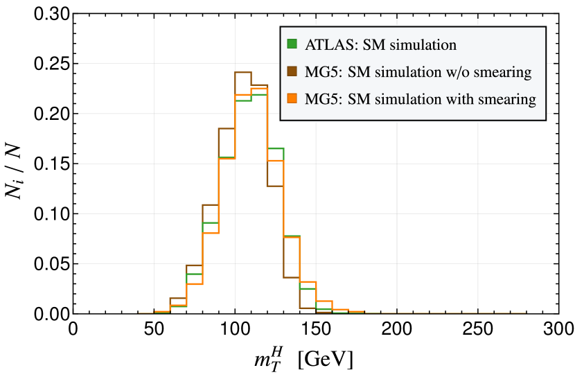
We simulated in this setup the process , with , and the tau lepton subsequently decaying, using MadGraph5aMC@NLO (MG5) [56], Pythia8.3 [57], and Delphes [58]. For each point in parameter space that we will consider in the following, we generated a sample containing one million events. In order to validate and correct our fast simulation, we first simulated the SM Higgs boson signal, i.e. , and compared the result to the ATLAS one for the SM Higgs boson signal given as a function of the transverse mass in Fig. 11 in Ref. [42].222Note that the definitions of ATLAS and CMS are slightly different (for instance, they contain details on the missing energy) and that we do not use the di-lepton invariant mass here as it is fully correlated to the transverse mass, the latter, however, containing more information. For this, we normalized the events per bin to the total number of events and then calculated the sum of the square of the differences between the two simulations of all bins , where MG5 stands for our MadGraph5aMC@NLO simulation. It turns out that to better match the distribution of ATLAS with our fast simulation, a smearing on the missing transverse energy to broaden the spectrum is necessary, as well as a shift of the to adjust the position of the peak. We thus uniformly generate random numbers and on a disk in the plane, i.e., with in units of GeV, between 0 and 1 and between 0 and . We then add the resulting values to the missing generated. In fact, we found that the best fit, i.e. minimal value for is obtained for 20 GeV. In addition, a shift of 3.5 GeV on the transverse mass leads to a very good agreement between our simulation and the one of ATLAS (see Fig. 2).
Next, we look at the production cross section and the efficiency of our simulation compared to the ATLAS one. First, note that in the ATLAS graph, the fitted signal (i.e. the one that agrees best with data, not taking into account the overall normalization from the SM theory prediction) is shown, such that one has to rescale the number of events by dividing by 1.21. We then corrected for the leading order MG5 simulation using an effective coupling. The resulting production cross section is 17.62 pb, while including NNLO corrections,333Since we consider the 0-jet category, hard jet emission is vetoed. Therefore, corrections are only relevant for the production cross section, which is however fitted in our approach. the CERN yellow report [59] quotes 48.57 pb. We also corrected for the simulation efficiency, i.e., the percentage of events left after applying the cuts, which in our analysis is while ATLAS finds , being in reasonable agreement.
We proceeded in a similar way for the CMS analysis, both for the GeV and the GeV categories (where stands for the transverse momentum of the subleading lepton) shown in Fig. 1 of Ref. [41]. Here, a smearing of GeV gives the best fit, while a shift is not necessary. For the production cross section, the same correction factor applies, while for the combined efficiency (GeV and GeV category), we find while CMS finds , again in reasonable agreement.444The difference in the efficiency of our fast simulation compared to the full simulation of ATLAS and CMS can be explained by pileup reducing the (unrealistically) high electron and muon efficiency of in Delphes, compared to the one of ATLAS and CMS for medium energetic leptons [60] as well as the full jet veto used.
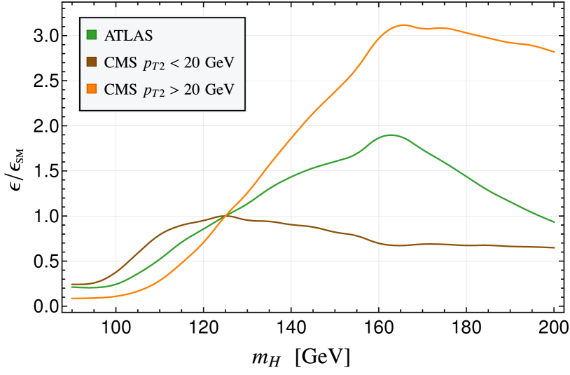
The dependence of the efficiency (relative to the SM) on is shown in Fig. 3.
For the BSM analysis, we will then apply the correction factors, as well as the smearing, determined from the SM Higgs boson. For the shift in , we assumed that it is proportional to the scalar mass .
III Analysis
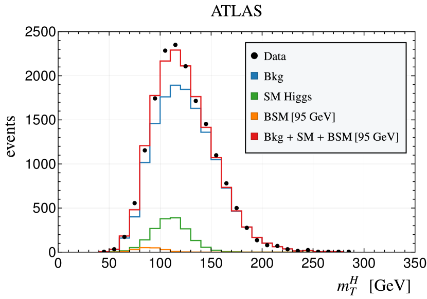
For the ATLAS analysis [42], we digitized the data points as well as the backgrounds and the SM Higgs boson signal for the 0-jet category555Here, we do not include the 1-jet and 2-jet categories. This is motivated by the fact that the multilepton anomalies include the production of opposite-sign leptons in association with jets, thus contaminating the control samples used to normalize the backgrounds in the 1-jet and 2-jet categories [24, 32]. Note that these categories are anyway less sensitive than the 0-jet one for the gluon-gluon fusion signal considered here. as a function of the transverse mass (Fig. 11 in the ATLAS paper). Concerning the latter, ATLAS scaled the theory prediction by 1.21 in order to obtain the best fit. As we study BSM effects, we, therefore, divided this contribution by this factor. For the statistical errors, we used the square root of the measured number of events per bin. Concerning the systematic error, one can see that there is a strong anti-correlations among the different background signals (including the SM Higgs boson signal) in Table 5 of the ATLAS paper. As the details of the (anti-)correlations are not given in the ATLAS paper, and the error on the Mis-Id background matches the total error, we chose this to be the experimental systematic error, also because it is reasonably the least correlated one with respect to the other backgrounds (which depend mostly on the detector efficiencies for leptons). Concerning the theory uncertainty, we included a 7% error on the SM Higgs boson signal (see Table 6 in Ref. [41]). Furthermore, we assumed both systematic errors to be uncorrelated from each other but fully correlated among the different bins.
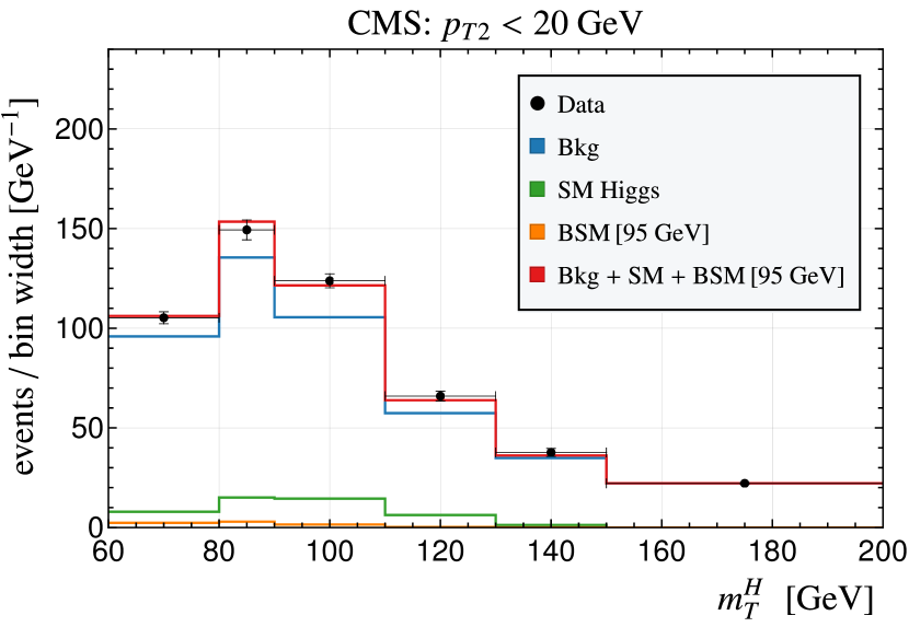
Analogously to the ATLAS procedure, we digitized the distributions for the GeV and GeV categories in Fig. 1 of Ref. [41]. However, CMS uses a different method for determining background and signal, namely a combined fit to data. Therefore, in the presence of a BSM signal, we allowed for refitting the SM background (including the SM Higgs boson signal) by a common factor , which can however be different for the two categories GeV and the GeV. This at the same time takes into account the experimental systematic uncertainties of the main background and the SM Higgs boson. Since for CMS, the systematic error on the nonprompt background is not given, we used as for the ATLAS analysis. On top of this, we included systematic theory error of the SM Higgs boson signal, the latter fully correlated among the GeV and the GeV categories and with the theory uncertainty for the ATLAS analysis.
The statistical model for the combined analysis is then built up with binned templates from observed data and expectations, including a possible BSM signal. In order to obtain the best-fit value of BSM signal strength, a simultaneous fit based on distribution is performed. For this, we calculate a common depending on the BSM signal,
| (1) |
where is the covariance matrix, is the number of measured events per bin, and
| (2) |
is composed of the background (BKG) events, the number of events expected within the SM, and the BSM component, with each contribution weighted by a respective fit parameter. We normalized the number of BSM events to the number of events within the SM, i.e., such that
| (3) |
While in Table V, we will give also separately for ATLAS, CMS with GeV and CMS with GeV, in our final combined fit, we will require it to be equal for all three categories.
IV Results
By minimizing the global function, a best-fit value of can be derived, and the corresponding value is then compared to the SM value . For the latter, a subtlety arises in the case of the CMS analyses: one can either use the value obtained directly from the CMS plots or allow for refitting the backgrounds, as done for the BSM analysis. While the latter option is more conservative, the first option seems more appropriate in the case of a nonzero BSM signal. We will therefore give both numbers in the following.
First, let us look at the results for the particularly interesting case of GeV and GeV, which are motivated by the anomalies mentioned in the introduction. The result is illustrated in Fig. 4 for a mass of GeV, and the numbers for both cases are given in Table V, where both the individual as well as the combined fit results are shown. In the leftmost part of the table, one can find the best-fit values for the parameters. The middle (rightmost) parts correspond to results in which the for the SM hypothesis is obtained with (without) refitting the background and the SM signal for the CMS analyses.
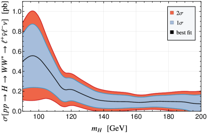
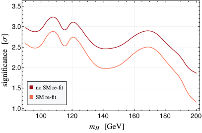
Finally, we show the preferred range of the cross section of as a function of from GeV up to GeV in Fig. 5, where we scanned over the mass in steps of GeV and then interpolated. The black line denotes the best fit while blue and red correspond to the and regions, respectively. The largest possible cross section is allowed for GeV and also at larger masses there is room for a BSM signal. Note that in the left plot of Fig. 5, we defined the and regions w.r.t. the best-fit values of the BSM scenario, allowing for a refit of the SM background for CMS even in case of a vanishing signal. Therefore, these regions correspond to the conservative approach discussed above.
V Conclusions and Outlook
rowsep=0.15cm
| [1.5pt] GeV | Sig. | Sig. | ||||||
| [1pt] ATLAS | 0.7 | 49.0 | 57.7 | 3.0 | 57.7 | 3.0 | ||
| CMS GeV | 1.01 | 0.0 | 5.5 | 5.5 | 0.0 | 6.8 | 1.2 | |
| CMS GeV | 1.01 | -3.5 | 6.2 | 9.0 | - | 9.1 | - | |
| Combined fit | 1.00 | 1.00 | 0.5 | 65.4 | 72.2 | 2.6 | 73.3 | 2.8 |
| [1pt] [0pt] [1pt] GeV | Sig. | Sig. | ||||||
| [1.5pt] ATLAS | 0.1 | 54.5 | 57.7 | 1.8 | 57.7 | 1.8 | ||
| CMS GeV | 0.97 | 0.6 | 1.5 | 5.5 | 2.0 | 6.8 | 2.3 | |
| CMS GeV | 0.99 | 0.2 | 8.0 | 9.0 | 1.0 | 9.1 | 1.0 | |
| Combined fit | 1.01 | 0.99 | 0.1 | 67.2 | 72.2 | 2.2 | 73.3 | 2.5 |
| [1.5pt] |
Motivated by the existing hints for new scalar particles with masses around GeV and GeV, we recast and combine the CMS and ATLAS analyses of the SM Higgs boson decaying into boson pairs to constrain light new scalars with a mass between 90 GeV and 200 GeV. In Fig. 5 we show the preferred and ranges for the corresponding cross section. Note that for the whole range, the observed limit is weaker than the expected one, resulting in a preference for nonzero BSM contribution. While the allowed cross section is largest around GeV, the global significance is only below . However, taking into account the existing hints for a GeV scalar in , the look-elsewhere effect is removed, and the global significance of our signal coincides with the local one of . Note that while for a GeV scalar there is already room for a positive signal in our setup with direct production, its production in association with missing energy is suggested by Refs. [25, 61] () and Refs. [62, 63] (). While such an associate production will broaden the values for , further increasing the significance, the quantification of this effect is outside the scope of this paper.
Due to the absence of a signal in the LHC analyses, our results suggest that the new scalar could be the neutral component of an triplet with hypercharge 0, that, at tree level and in the absence of mixing, only decays to a pair of bosons. This observation is interesting in light of the fact that this field can at the same time naturally account for the mass measurement of the CDF II Collaboration, in case its vacuum expectation value is around a few GeV.
Acknowledgements.
We thank Mukesh Kumar, Shuiting Xin, Salah-Eddine Dahbi and Saiyad Ashanujjaman for useful discussions. The work of A.C. is supported by a professorship grant of the Swiss National Science Foundation (Grant No. PP00P21_76884). B.M. gratefully acknowledges the South African Department of Science and Innovation through the SA-CERN program, the National Research Foundation, and the Research Office of the University of the Witwatersrand for various forms of support.References
- Zyla et al. [2020] P. A. Zyla et al. (Particle Data Group), Review of Particle Physics, PTEP 2020, 083C01 (2020).
- Amhis et al. [2021] Y. S. Amhis et al. (HFLAV), Averages of b-hadron, c-hadron, and -lepton properties as of 2018, Eur. Phys. J. C 81, 226 (2021), arXiv:1909.12524 [hep-ex] .
- Schael et al. [2006] S. Schael et al. (ALEPH, DELPHI, L3, OPAL, SLD, LEP Electroweak Working Group, SLD Electroweak Group, SLD Heavy Flavour Group), Precision electroweak measurements on the resonance, Phys. Rept. 427, 257 (2006), arXiv:hep-ex/0509008 .
- Higgs [1964a] P. W. Higgs, Broken symmetries, massless particles and gauge fields, Phys. Lett. 12, 132 (1964a).
- Englert and Brout [1964] F. Englert and R. Brout, Broken Symmetry and the Mass of Gauge Vector Mesons, Phys. Rev. Lett. 13, 321 (1964).
- Higgs [1964b] P. W. Higgs, Broken Symmetries and the Masses of Gauge Bosons, Phys. Rev. Lett. 13, 508 (1964b).
- Guralnik et al. [1964] G. S. Guralnik, C. R. Hagen, and T. W. B. Kibble, Global Conservation Laws and Massless Particles, Phys. Rev. Lett. 13, 585 (1964).
- Aad et al. [2012] G. Aad et al. (ATLAS), Observation of a new particle in the search for the Standard Model Higgs boson with the ATLAS detector at the LHC, Phys. Lett. B 716, 1 (2012), arXiv:1207.7214 [hep-ex] .
- Chatrchyan et al. [2012] S. Chatrchyan et al. (CMS), Observation of a New Boson at a Mass of 125 GeV with the CMS Experiment at the LHC, Phys. Lett. B 716, 30 (2012), arXiv:1207.7235 [hep-ex] .
- ATL [2022a] Combination of searches for heavy resonances using 139 fb-1 of proton–proton collision data at = 13 TeV with the ATLAS detector, Tech. Rep. (CERN, Geneva, 2022).
- Naryshkin [2021] Y. G. Naryshkin, Search for new heavy Higgs bosons in ATLAS and CMS experiments at LHC (Mini-review), Pisma Zh. Eksp. Teor. Fiz. 113, 221 (2021).
- Barate et al. [2003] R. Barate et al. (LEP Working Group for Higgs boson searches, ALEPH, DELPHI, L3, OPAL), Search for the standard model Higgs boson at LEP, Phys. Lett. B 565, 61 (2003), arXiv:hep-ex/0306033 .
- Sirunyan et al. [2019] A. M. Sirunyan et al. (CMS), Search for a standard model-like Higgs boson in the mass range between 70 and 110 GeV in the diphoton final state in proton-proton collisions at 8 and 13 TeV, Phys. Lett. B 793, 320 (2019), arXiv:1811.08459 [hep-ex] .
- CMS [2022a] Searches for additional Higgs bosons and vector leptoquarks in final states in proton-proton collisions at , Tech. Rep. (CERN, Geneva, 2022).
- CMS [2022b] Search for a new resonance decaying to two scalars in the final state with two bottom quarks and two photons in proton-proton collisions at , Tech. Rep. (CERN, Geneva, 2022).
- Cao et al. [2017] J. Cao, X. Guo, Y. He, P. Wu, and Y. Zhang, Diphoton signal of the light Higgs boson in natural NMSSM, Phys. Rev. D 95, 116001 (2017), arXiv:1612.08522 [hep-ph] .
- Biekötter et al. [2020] T. Biekötter, M. Chakraborti, and S. Heinemeyer, A 96 GeV Higgs boson in the N2HDM, Eur. Phys. J. C 80, 2 (2020), arXiv:1903.11661 [hep-ph] .
- Crivellin et al. [2018] A. Crivellin, J. Heeck, and D. Müller, Large in generic two-Higgs-doublet models, Phys. Rev. D 97, 035008 (2018), arXiv:1710.04663 [hep-ph] .
- Haisch and Malinauskas [2018] U. Haisch and A. Malinauskas, Let there be light from a second light Higgs doublet, JHEP 03, 135, arXiv:1712.06599 [hep-ph] .
- Fox and Weiner [2018] P. J. Fox and N. Weiner, Light Signals from a Lighter Higgs, JHEP 08, 025, arXiv:1710.07649 [hep-ph] .
- Heinemeyer [2018] S. Heinemeyer, A Higgs boson below 125 GeV?!, Int. J. Mod. Phys. A 33, 1844006 (2018).
- Biekötter et al. [2022] T. Biekötter, S. Heinemeyer, and G. Weiglein, Mounting evidence for a 95 GeV Higgs boson, JHEP 08, 201, arXiv:2203.13180 [hep-ph] .
- Iguro et al. [2022] S. Iguro, T. Kitahara, and Y. Omura, Scrutinizing the 95–100 GeV di-tau excess in the top associated process, Eur. Phys. J. C 82, 1053 (2022), arXiv:2205.03187 [hep-ph] .
- von Buddenbrock et al. [2018] S. von Buddenbrock, A. S. Cornell, A. Fadol, M. Kumar, B. Mellado, and X. Ruan, Multi-lepton signatures of additional scalar bosons beyond the Standard Model at the LHC, J. Phys. G 45, 115003 (2018), arXiv:1711.07874 [hep-ph] .
- Aad et al. [2021a] G. Aad et al. (ATLAS), Search for dark matter in events with missing transverse momentum and a Higgs boson decaying into two photons in pp collisions at = 13 TeV with the ATLAS detector, JHEP 10, 013, arXiv:2104.13240 [hep-ex] .
- Crivellin et al. [2021] A. Crivellin, Y. Fang, O. Fischer, A. Kumar, M. Kumar, E. Malwa, B. Mellado, N. Rapheeha, X. Ruan, and Q. Sha, Accumulating Evidence for the Associate Production of a Neutral Scalar with Mass around GeV (2021) arXiv:2109.02650 [hep-ph] .
- Richard [2021] F. Richard, A Georgi-Machacek Interpretation of the Associate Production of a Neutral Scalar with Mass around 151 GeV (2021) arXiv:2112.07982 [hep-ph] .
- Fowlie [2022] A. Fowlie, Comment on: Accumulating evidence for the associate production of a neutral scalar with mass around 151 GeV, Phys. Lett. B 827, 136936 (2022), arXiv:2109.13426 [hep-ph] .
- Sirunyan et al. [2017] A. M. Sirunyan et al. (CMS), Measurements of properties of the Higgs boson decaying into the four-lepton final state in pp collisions at TeV, JHEP 11, 047, arXiv:1706.09936 [hep-ex] .
- Aad et al. [2021b] G. Aad et al. (ATLAS), Search for resonances decaying into photon pairs in 139 fb-1 of collisions at =13 TeV with the ATLAS detector, Phys. Lett. B 822, 136651 (2021b), arXiv:2102.13405 [hep-ex] .
- Consoli and Cosmai [2022] M. Consoli and L. Cosmai, Experimental signals for a second resonance of the Higgs field, Int. J. Mod. Phys. A 37, 2250091 (2022), arXiv:2111.08962 [hep-ph] .
- Buddenbrock et al. [2019] S. Buddenbrock, A. S. Cornell, Y. Fang, A. Fadol Mohammed, M. Kumar, B. Mellado, and K. G. Tomiwa, The emergence of multi-lepton anomalies at the LHC and their compatibility with new physics at the EW scale, JHEP 10, 157, arXiv:1901.05300 [hep-ph] .
- von Buddenbrock et al. [2020] S. von Buddenbrock, R. Ruiz, and B. Mellado, Anatomy of inclusive production at hadron colliders, Phys. Lett. B 811, 135964 (2020), arXiv:2009.00032 [hep-ph] .
- Hernandez et al. [2021] Y. Hernandez, M. Kumar, A. S. Cornell, S.-E. Dahbi, Y. Fang, B. Lieberman, B. Mellado, K. Monnakgotla, X. Ruan, and S. Xin, The anomalous production of multi-lepton and its impact on the measurement of production at the LHC, Eur. Phys. J. C 81, 365 (2021), arXiv:1912.00699 [hep-ph] .
- Fischer et al. [2022] O. Fischer et al., Unveiling hidden physics at the LHC, Eur. Phys. J. C 82, 665 (2022), arXiv:2109.06065 [hep-ph] .
- von Buddenbrock et al. [2016] S. von Buddenbrock, N. Chakrabarty, A. S. Cornell, D. Kar, M. Kumar, T. Mandal, B. Mellado, B. Mukhopadhyaya, R. G. Reed, and X. Ruan, Phenomenological signatures of additional scalar bosons at the LHC, Eur. Phys. J. C 76, 580 (2016), arXiv:1606.01674 [hep-ph] .
- von Buddenbrock et al. [2019] S. von Buddenbrock, A. S. Cornell, E. D. R. Iarilala, M. Kumar, B. Mellado, X. Ruan, and E. M. Shrif, Constraints on a 2HDM with a singlet scalar and implications in the search for heavy bosons at the LHC, J. Phys. G 46, 115001 (2019), arXiv:1809.06344 [hep-ph] .
- CMS [2022c] Search for high mass resonances decaying into in the dileptonic final state with of proton-proton collisions at , Tech. Rep. (CERN, Geneva, 2022).
- ATL [2022b] Search for heavy resonances in the decay channel in Collisions at 13 TeV using 139 fb-1 of data with the ATLAS detector, Tech. Rep. (CERN, Geneva, 2022).
- Sirunyan et al. [2020] A. M. Sirunyan et al. (CMS), Search for a heavy Higgs boson decaying to a pair of bosons in proton-proton collisions at 13 TeV, JHEP 03, 034, arXiv:1912.01594 [hep-ex] .
- CMS [2022d] Measurements of the Higgs boson production cross section and couplings in the WW boson pair decay channel in proton-proton collisions at 13 TeV, Tech. Rep. (CERN, Geneva, 2022) arXiv:2206.09466 .
- ATL [2022c] Measurements of Higgs boson production by gluon-gluon fusion and vector-boson fusion using decays in collisions at TeV with the ATLAS detector, Tech. Rep. (CERN, Geneva, 2022) arXiv:2207.00338 .
- Rizzo [1991] T. G. Rizzo, Updated bounds on Higgs triplet vacuum expectation values and the tree level rho parameter from radiative corrections, Mod. Phys. Lett. A 6, 1961 (1991).
- Chardonnet et al. [1993] P. Chardonnet, P. Salati, and P. Fayet, Heavy triplet neutrinos as a new dark matter option, Nucl. Phys. B 394, 35 (1993).
- Blank and Hollik [1998] T. Blank and W. Hollik, Precision observables in models with an additional Higgs triplet, Nucl. Phys. B 514, 113 (1998), arXiv:hep-ph/9703392 .
- Fileviez Perez et al. [2022] P. Fileviez Perez, H. H. Patel, and A. D. Plascencia, On the mass and new Higgs bosons, Phys. Lett. B 833, 137371 (2022), arXiv:2204.07144 [hep-ph] .
- Rizzo [2022] T. G. Rizzo, Kinetic mixing, dark Higgs triplets, and , Phys. Rev. D 106, 035024 (2022), arXiv:2206.09814 [hep-ph] .
- Wang et al. [2022] J.-W. Wang, X.-J. Bi, P.-F. Yin, and Z.-H. Yu, Electroweak dark matter model accounting for the CDF -mass anomaly, Phys. Rev. D 106, 055001 (2022), arXiv:2205.00783 [hep-ph] .
- Cheng et al. [2022] Y. Cheng, X.-G. He, F. Huang, J. Sun, and Z.-P. Xing, Electroweak precision tests for triplet scalars (2022) arXiv:2208.06760 [hep-ph] .
- Song et al. [2022] H. Song, X. Wan, and J.-H. Yu, Custodial Symmetry Violation in Scalar Extensions of the Standard Model (2022) arXiv:2211.01543 [hep-ph] .
- Aaltonen et al. [2022] T. Aaltonen et al. (CDF), High-precision measurement of the boson mass with the CDF II detector, Science 376, 170 (2022).
- de Blas et al. [2022] J. de Blas, M. Ciuchini, E. Franco, A. Goncalves, S. Mishima, M. Pierini, L. Reina, and L. Silvestrini, Global analysis of electroweak data in the Standard Model, Phys. Rev. D 106, 033003 (2022), arXiv:2112.07274 [hep-ph] .
- Bagnaschi et al. [2022] E. Bagnaschi, J. Ellis, M. Madigan, K. Mimasu, V. Sanz, and T. You, SMEFT analysis of , JHEP 08, 308, arXiv:2204.05260 [hep-ph] .
- Chabab et al. [2018] M. Chabab, M. C. Peyranère, and L. Rahili, Probing the Higgs sector of Higgs Triplet Model at LHC, Eur. Phys. J. C 78, 873 (2018), arXiv:1805.00286 [hep-ph] .
- Cacciapaglia et al. [2022] G. Cacciapaglia, T. Flacke, M. Kunkel, W. Porod, and L. Schwarze, Exploring extended Higgs sectors via pair production at the LHC, JHEP 12, 087, arXiv:2210.01826 [hep-ph] .
- Alwall et al. [2014] J. Alwall, R. Frederix, S. Frixione, V. Hirschi, F. Maltoni, O. Mattelaer, H. S. Shao, T. Stelzer, P. Torrielli, and M. Zaro, The automated computation of tree-level and next-to-leading order differential cross sections, and their matching to parton shower simulations, JHEP 07, 079, arXiv:1405.0301 [hep-ph] .
- Sjöstrand et al. [2015] T. Sjöstrand, S. Ask, J. R. Christiansen, R. Corke, N. Desai, P. Ilten, S. Mrenna, S. Prestel, C. O. Rasmussen, and P. Z. Skands, An introduction to PYTHIA 8.2, Comput. Phys. Commun. 191, 159 (2015), arXiv:1410.3012 [hep-ph] .
- de Favereau et al. [2014] J. de Favereau, C. Delaere, P. Demin, A. Giammanco, V. Lemaître, A. Mertens, and M. Selvaggi (DELPHES 3), DELPHES 3, A modular framework for fast simulation of a generic collider experiment, JHEP 02, 057, arXiv:1307.6346 [hep-ex] .
- de Florian et al. [2017] D. de Florian et al. (LHCHiggsCrossSectionWorkingGroup), Handbook of LHC Higgs Cross Sections: 4. Deciphering the Nature of the Higgs Sector, CERN Yellow Reports: Monographs (CERN, Geneva, 2017).
- Jain [2021] S. Jain (ATLAS, CMS), Lepton and Photon reconstruction and identification performance in ATLAS and CMS in Run II, PoS LHCP2020, 046 (2021).
- ATL [2023] Model-independent search for the presence of new physics in events including with = 13 TeV pp data recorded by the ATLAS detector at the LHC, Tech. Rep. (CERN, Geneva, 2023) arXiv:2301.10486 .
- Aad et al. [2021c] G. Aad et al. (ATLAS), Search for Dark Matter Produced in Association with a Dark Higgs Boson Decaying into or in Fully Hadronic Final States from TeV pp Collisions Recorded with the ATLAS Detector, Phys. Rev. Lett. 126, 121802 (2021c), arXiv:2010.06548 [hep-ex] .
- ATL [2022d] Search for dark matter produced in association with a dark Higgs boson decaying into in the one-lepton final state at TeV using 139 fb-1 of collisions recorded with the ATLAS detector, Tech. Rep. (CERN, Geneva, 2022) arXiv:2211.07175 .