On global solvability of a class of possibly nonconvex QCQP problems in Hilbert spaces

Abstract.

We provide conditions ensuring that the KKT-type conditions characterizes the global optimality for quadratically constrained (possibly nonconvex) quadratic programming QCQP problems in Hilbert space. The key property is the convexity ofa image-type set related to the functions appearing in the formulation of the problem. The proof of the main result relies on a generalized version of the (Jakubovich) S-Lemma in Hilbert spaces. As an application, we consider the class of QCQP problems with a special form of the quadratic terms of the constraints.
Keywords: Global solvability, QCQP problems, KKT conditions, Jakubovich lemma, S-lemma, image set
MSC2020: 90C20, 90C23, 90C26, 90C46

1. Introduction

The aim of this work is to establish a sufficient condition under which the KKT-type conditions characterizes the global optimality of a possibly non convex Quadratically Constrained Quadratic Programming (QCQP) problem in Hilbert spaces.

Let $H$ be a Hilbert space with the inner product $\langle a,b\rangle$, for $a,b\in H$, and the associated norm $\|\cdot\|=\sqrt{\langle\cdot,\cdot\rangle}$.

A generic QCQP problem is defined as follows.

$$\begin{split}&{Minimize\,}_{x\in H}\ \ J(x):=\langle x,A_{J}x\rangle+2\langle b_{J},x\rangle+c_{J}\\ &s.t.\ \ f_{k}(x):=\langle x,A_{k}x\rangle+2\langle b_{k},x\rangle+c_{k}\leq 0,\ \ k=1,...,m\end{split}$$ (QCQP)

where the continuous linear self-adjoint operators $A_{J},A_{k}:H\rightarrow H$, $b_{J},b_{k}\in H$, and $c_{J},c_{k}\in\mathbb{R}$ are given data for $k=1,...,m$.

Problems of the form QCQP (constrained and unconstrained) appear in many contexts. For a recent application in succesive quadratic approximation method, see [20]. In $\mathbb{R}^{n}$, QCQP problems also appear in the discretization of ill-posed problems, [11], maximum clique problem, [17], the circular packing problem, [29] and the Chebyshev center problem, [32]. Regarding Hilbert spaces, quadratic problems arise in calculus of variations, [14], in optimal control, [33] and in in the context of reproducing kernel Hilbert space, [27].

We consider both general QCQP problems and a special class of QCQP problems which satisfy the following assumption:

Assumption 1.

Let $A_{J},A_{k}$ $\forall\,k\in\{1,...,m\}$ be of the form $A_{J}=a_{J}I,A_{k}=a_{k}I$, where $a_{J},a_{k}\in\mathbb{R}$ and $I$ is the identity operator.

When Assumption 1 holds, QCQP takes the form

$$\begin{split}&{Minimize\,}_{x\in H}\ \ J(x):=a_{J}\|x\|^{2}+2\langle b_{J},x\rangle+c_{J}\\ &s.t.\ \ f_{k}(x):=a_{k}\|x\|^{2}+2\langle b_{k},x\rangle+c_{k}\leq 0,\ \ k=1,...,m\end{split}$$ (S-QCQP)

Since in S-QCQP the operators $A_{J},A_{k}$, $A_{J},A_{k}$ $k=1,...,m$ do not appear and instead we only have the scalars $a_{J},a_{k}\in\mathbb{R}$, $k=1,...,m$, in the sequel we refer to S-QCQP as the scalar QCQP.

Remark 1.

The scalars $a_{J},a_{k}$, $k=1,...,m$ can be equal to zero for S-QCQP. When $a_{J}=0$ and/or $a_{k}=0$ for some $k$, the corresponding $J(x)$ or $f_{k}(x)$ are linear forms. In case $a_{J}=0$ and/or $a_{k}=0$ for all $k$, S-QCQP become a linear or a quadratic convex optimization problem, respectively. ∎

Definition 1.

Given a self-adjoint linear continous operator $A$ (i.e. $\langle Ax,x\rangle=\langle x,Ax\rangle$), the quadratic form ${A(x):=\langle x,Ax\rangle}$ is said to be positive if $\langle x,Ax\rangle>0$, $\forall\,x\in H\setminus\{0\}$ and non negative if $\langle x,Ax\rangle\geq 0$, $\forall\,x\in H$.∎

By Proposition 3.71 of [4], a quadratic form $\langle x,Ax\rangle+2\langle b,x\rangle+c$ is convex if and only if $A(x):=\langle x,Ax\rangle$ is non negative.

We say that KKT conditions for QCQP are satisfied at a feasible point $x^{*}$ if there exists $\gamma=(\gamma_{1},...,\gamma_{m})$, $\gamma_{i}\geq 0$, $m=1,...,m$ such that

$$\begin{split}&(i)\ \ \ \nabla(J+\sum\limits_{k=1}^{m}\gamma_{k}f_{k})(x^{*})=0,\text{stationarity}\\ &(ii)\ \ \gamma_{k}f_{k}(x^{*})=0\ \ k\in\{1,...,m\},\text{complementarity}\\ &(iii)\ (A_{J}+\sum\limits_{k=1}^{m}\gamma_{k}A_{k})(x)\text{ non negative}.\end{split}$$ (KKT)

Then, the optimal value of (QCQP) is $J^{*}=J(x^{*})$.

In general, under standard constraint qualification ( e.g. Mangasarian-Fromowitz CQ) KKT conditions are necessary for local optimality of $x^{*}$ for QCQP, see Theorem 3.6 of [30].

In this paper, we determine conditions under which KKT are necessary and sufficient global optimality conditions in Hilbert spaces for QCQP, section 3, and S-QCQP, section 4.

The authors of [18] prove that KKT are necessary and sufficient optimality conditions in $\mathbb{R}^{n}$ for QCQP problems if the matrices $H_{J}:=\begin{pmatrix}A_{J}&b_{J}\\ b_{J}^{T}&c_{J}\end{pmatrix}$ and $H_{k}:=\begin{pmatrix}A_{k}&b_{k}\\ b_{k}^{T}&c_{k}\end{pmatrix}$ $\forall\,k\in\{1,...,m\}$ are $Z$-matrices. $Z$-matrices are matrices with non positive off diagonal elements. In order to characterize the optimal value of Z-matrices QCQP, in [18] the authors propose a generalized version of the S-Lemma for $Z$-matrices QCQP, in the sense described in Section 2.

We apply the approach similar to that proposed in [18] and we base our developments on a generalized version of the S-Lemma in Hilbert spaces. The key property is the convexity of the Generalized Image Set

$$\Omega_{0}:=\{(f_{0}(x),f_{1}(x),...,f_{m}(x))\ |\ x\in H\}+int\mathbb{R}^{m+1}_{+},$$ (GIS)

$f_{0}:=J(x)-J^{*}$ and ${}^{\prime}+^{\prime}$ is the Minkowski sum of the range $\{(f_{0}(x),f_{1}(x),...,f_{m}(x))\ |\ x\in H\}$ and the interior of the cone $\mathbb{R}^{m+1}_{+}$. By [16], exercise 2.1, the set $\Omega_{0}$ is open. Recall, that the image set of optimization problems defined as

$$\{(f_{0}(x),f_{1}(x),...,f_{m}(x))\ |\ x\in H\}$$ (1.1)

has been extensively investigated in the monograph by [10]. In [18], it is shown that (1.1) is not sufficient to establish if the KKT conditions are necessary and sufficient for global optimality of every class of QCQP. They consider instead GIS.

Showing the convexity of [10] or of GIS is a key step in the proof of the famous Jakubovich S-Lemma, [33].

The S-Lemma is an important result related to the general S-procedure described in [9], treated from an historical point view in [13]. Paper [24] provides a comprehensive survey on the S-Lemma in $\mathbb{R}^{n}$, while [19] explores the relations between the S-Lemma and the Lagrangian multipliers of QCQP. In [1], an S-Lemma based approach similar to the one proposed by [18] and the present paper is applied to problem with data uncertainty in $\mathbb{R}^{n}$. The paper [26] extend the results of [18] to Z-matrices QCQP in $\mathbb{R}^{n}$ with infinite number of inequalities. More recent generalization of the S Lemma in $\mathbb{R}^{n}$ appear in [31], [28]. Also in these latter papers, the sets (1.1) and GIS play an important role.

In $\mathbb{R}^{n}$, the convexity of the set $\Omega_{0}$ for (S-QCQP) is proved in [3], when $m+1\leq n$. For (QCQP) with one or two constraints, i.e. $m=1$ and $m=2$, the convexity of $\Omega_{0}$ can be proved under some regularity conditions, starting from the results of Dine and Polyak (see [18], [24]). For Z-matrices QCQP, the convexity of $\Omega_{0}$ is proved in [18].

In [6], the results of Dine and Polyak are generalized in Hilbert spaces. As a conseguence, a generalized form of the S-Lemma for three homogeneous quadratic functionals, i.e. $f_{k}(x):=\langle x,A_{k}x\rangle$, $k=0,1,2$, holds in Hilbert spaces.

Other results concerning generalized S-Lemma in Hilbert spaces for homogeneous quadratic functionals can be found in [33].

In section 3, we prove that, for general (QCQP) in Hilbert space, if $\Omega_{0}$ is convex, then the generalized S-Lemma holds and the (KKT) conditions are necessary and sufficient for global optimality.

Throughout the whole paper, we are making the following existence assumption.

Assumption 2.

There exists a global minimum $x^{*}$ of problem QCQP and there exists $\gamma\in\mathbb{R}^{m}_{+}\backslash\ 0$ such that $(A_{J}+\sum\limits\gamma_{k}A_{k})(x)$ is non negative.

The assumption $\exists\,\gamma\in\mathbb{R}^{m}_{+}\backslash\ 0$ such that the matrix $A_{J}+\sum\limits\gamma_{k}A_{k}\succeq 0$, is a standard assumption in the literature related to finite dimensional QCQP, see e.g. [21], [22] and [23]. Observe that it is non verified by nonconvex QP (quadratic problems with linear constraints only), since $A_{J}\not\succeq 0$. KKT conditions and the SDP relaxation for QP in $\mathbb{R}^{n}$ are studied e.g. in [12], [5].

The assumption that there exists a global minimum $x^{*}$ of problem QCQP, it is made to avoid discussing the existence of solution for QCQP problems in Hilbert spaces, which is covered by other papers (see e.g. [8]). When we will explicitly calculate the KKT conditions for S-QCQP, we will assume the objective function to be $J(x):=\|x-z\|^{2}$, $z\in H$ to guarantee the existence of a solution on a closed, but possibly non convex, constrained set.

For convex QP problems (quadratic convex objective functions under linear constraints only) in Hilbert spaces, conditions for the existence of solutions and global optimality conditions can be found respectively in Theorem 3.128 and Theorem 3.130 of [4].

The organization of the paper is as follows. In Section 2, we provide the preliminaries concerning the notation, the S-Lemma, the Fermat rule and the convex separation theorem which are used in the sequel.

The main result of Section 3 is Theorem 8, which provides the global minima characterization for general QCQP problems in the form of KKT conditions, under the assumption that $\Omega_{0}$ is convex.

In Section 4, we apply Theorem 8 to provide a characterization of the global solution for S-QCQP. The main result is Theorem 11 which proves the convexity of the set $\Omega_{0}$ for this class of QCQP problems.

2. Preliminaries

Given a vector $x\in\mathbb{R}^{n}$, we say $x\geq 0$ when every component is non-negative and we define ${\mathbb{R}^{n}_{+}:=\{x\in\mathbb{R}^{n}\ |\ x\geq 0\}}$. $0$ may also denotes the all-zero vector in $H$. Given two vectors $x,y\in H$, $\langle x,y\rangle$ denotes the inner product between $x$ and $y$. When $x=\mathbb{R}^{n}$, we have $\langle x,y\rangle=x^{T}y=y^{T}x$. The corresponding norm is denoted by $\|\cdot\|=\sqrt{\langle\cdot,\cdot\rangle}$.

Let $S^{n}$ be the set of symmetric matrices in $\mathbb{R}^{n\times n}$. $S^{n}_{+}$ and $S^{n}_{++}$ are the cones of symmetric matrices which are also positive semidefinite and positive definite, respectively. If a matrix $A$ belongs to $S^{n}_{+}$ then we write $A\succeq 0$; if $A\in S^{n}_{++}$ then we write $A\succ 0$.

By $diag(A)\in\mathbb{R}^{n}$, we denote the vector of the elements in the main diagonal of $A\in\ S^{n}$. The trace inner product $\langle A,B\rangle$, between symmetric matrices $A$, $B$ of dimension $n\times n$ is defined as $\langle A,B\rangle:=Tr(B^{T}A)=\sum_{i=1}^{n}\sum_{j=1}^{n}a_{ij}b_{ij}$. Let $|\cdot|$ denote the cardinality of a set. $C$ is an affine subspace if $C\neq\emptyset$ and $\forall\,\lambda\in\mathbb{R}$ and for all distinct $x,y\in C$

$$\lambda x+(1-\lambda)y\in C$$

$\textit{aff}\,C$ denotes the affine hull of $C$, i.e. the smallest affine subspace of $H$ containing $C$, $int\,C$ denotes the interior of $C$,

$$int\,C:=\{x\in C\,|\,(\exists\,\epsilon>0)\,(x+\epsilon B_{1})\subset C\}.$$

$B_{1}:=\{x\,|\,\|x\|\leq 1\}$ be the unit ball in $H$. The relative interior of $C$, denoted $ri\,C$, can be espressed in $\mathbb{R}^{n}$ as :

$$ri\,C:=\{x\in\textit{aff}\,C\,|\,(\exists\,\epsilon>0)\,(x+\epsilon B_{1})\cap(\textit{aff}\,C)\subset C\}.$$ (2.1)

2.1. Jakubovich S-Lemma, basic separation theorem

An important theorem for the optimality conditions of QCQP is the S-lemma. We recall a generalized version of the S-Lemma that can be found in [24].

Theorem 1.

(Jakubovich S-Lemma) Let $f,g:\mathbb{R}^{n}\to\mathbb{R}$ be quadratic functionals and suppose that there exists a point $x_{0}\in\mathbb{R}$ such that $g(x_{0})<0$. The following statements (i) and (ii) are equivalent.

$$(i)\ \ (\nexists\,x\in\mathbb{R}^{n})\ \ s.t.\ \ f(x)<0\ \ g(x)\leq 0$$

$$(ii)\ \ \exists\gamma\geq 0\,\,\,such\,\,\,that\,\,\,f(x)+\gamma g(x)\geq 0\,\,\,\forall x\in\mathbb{R}^{n}$$

Consider a collection of quadratic functionals ${f_{k}:H\to\mathbb{R}}$ ${(k=1,...,m)}$. A theorem of the alternative is called generalized version of the S-Lemma if it establishes the conditions on the functionals $f_{k}$ under which only one between the following statements holds:

1. $\exists\,x\in H$ such that $f_{k}(x)<0\ \ \forall\,k\in\{1,...,m\}$

2. $(\exists\,\gamma\in\mathbb{R}_{+}^{m}\backslash 0)$ $\sum\limits_{k=1}^{m}\gamma_{k}f_{k}(x)\geq 0$ $\forall\,x\in H$

Let $\partial\,f(x)$ denote the convex subdifferential of $f$ at $x$, then we write $v\in\partial\,f(x)$ if

$$f(y)-f(x)\geq\langle v,y-x\rangle\quad\forall\,y\in H.$$ (2.2)

If $f$ is differentiable and convex, $\partial\,f(x)=\{\nabla f(x)\}$. By (2.2), it is possible to prove the Fermat’s optimality condition, see e.g. Theorem 16.3 of [2].

Theorem 2.

(Fermat optimality conditions) Let $f:H\rightarrow\ ]-\infty,+\infty]$ be proper. Then

$$Arg\,min\,f=\{x\in H\ |\ 0\in\partial f(x)\}.$$

Let $C_{1}$ and $C_{2}$ be non-empty subsets in $\mathbb{R}^{n}$.

Definition 2.

([25], section 11)

• A hyperplane $P$ is said to separate $C_{1}$ and $C_{2}$ if $C_{1}$ is contained in one of the closed half spaces associated to $P$ and $C_{2}$ is contained in the opposite closed half space.

• $P$ is said to separate properly $C_{1}$ and $C_{2}$ if they are not both contained in $P$ itself.

We are ready to state the convex separation theorem in finite dimensions, that will be crucial in the next section.

Theorem 3.

([25], Theorem 11.3)

Let $C_{1}$ and $C_{2}$ be non-empty convex sets in $\mathbb{R}^{n}$. In order that there exists a hyperplane that separates $C_{1}$ and $C_{2}$ properly, it is necessary and sufficient that $ri\,C_{1}$ and $ri\,C_{2}$ have no point in common.

For $n$-dimensional convex sets in $\mathbb{R}^{n}$, $\textit{aff}\,C=\mathbb{R}^{n}$ and so, by (2.1), we have $ri\,C=int\,C$ ([25], section 6).

Hence, we can rewrite Theorem 3 as follows.

Theorem 4.

Let $C_{1}$ and $C_{2}$ be $n$-dimensional non-empty convex sets in $\mathbb{R}^{n}$. In order that there exists a hyperplane that separates $C_{1}$ and $C_{2}$ properly, it is necessary and sufficient that $int\,C_{1}$ and $int\,C_{2}$ have no point in common.

2.2. Direct sum decompositions in Hilbert spaces

We apply the following concepts and results in the fourth section of the present work. This subsection is based on the monograph [7].

If $H_{1}$ and $H_{2}$ are subspaces of a Hilbert space $H$ we write ${H=H_{1}\oplus H_{2}}$ if each $x\in H$ has a unique representation in the form $x=x_{1}+x_{2}$, where $x_{1}\in H_{1}$ and $x_{2}\in H_{2}$. ${H_{1}\oplus H_{2}}$ is the direct sum of $H_{1}$ and $H_{2}$. If $H_{1}$ is a closed subspace of $H$, one can always find a subspace $H_{2}$ such that ${H=H_{1}\oplus H_{2}}$, $H_{2}$ is called a complement to $H_{1}$ and is orthogonal to $H_{1}$, $H_{2}=H_{1}^{\perp}$, i.e. $\langle x_{1},x_{2}\rangle=0$, for any $x_{1}\in H_{1}$, $x_{2}\in H_{2}$.

Definition 3.

Given a finite dimensional subset $H_{1}$ of a Hilbert space $H$, a basis of $H_{1}$ is a set of maximal linearly indipendent vectors $y_{k}\in H_{1}$, $k=1,2,..,m$, $m\in\mathbb{N}$ such that every vector $y$ of $H_{1}$ can be represented as $\sum\limits_{k=1}^{m}\alpha_{k}y_{k}$. We say that the set of vectors $y_{k}\in H$, $k=1,2,..,m$, $m\in\mathbb{N}$ spans $H_{1}$. The dimension of a subspace $H_{1}$ of $H$, denoted $\text{dim }H_{1}$, is equal the number of vectors in a basis of $H_{1}$.

Definition 4.

(Definition 7.9 from [7]) Let $H$ be a inner product space. A closed subspace $H_{1}$ of $H$ is said to have codimension $m<\infty$, written ${\text{codim }H_{1}=m}$, if there exists a subspace $H_{2}$ with $\text{dim }H_{2}=m$ such that $H=H_{1}\oplus H_{2}$.

The following results is a consequence of Theorem 7.11 and Theorem 7.12 from [7].

Theorem 5.

Let $H$ be a Hilbert space. Let $V$ be a closed subspace of $H$ and $m$ be a positive integer. Then, $\text{codim }V=m$ if and only if

$$V=\bigcap\limits_{i=1}^{m}\{x\in H\ |\ \langle b_{i},x\rangle=0\},$$

for some linearly independent set $\{b_{l},b_{2},\cdots,b_{m}\}$ in $H$.

We end this section with the following theorem on linear operators in Hibert spaces. Let us recall that, for a given linear continuous operator $A:H_{1}\rightarrow H_{2}$ acting between two Hilbert spaces $H_{1}$ and $H_{2}$,

$$\text{range}\,A:=\{y\in H_{2}\ |\ y=Ax\ \text{for some}\ x\in H_{1}\},\ \ \text{ker }A:=\{x\in H\ |\ Ax=0\}.$$

Let $\langle\cdot,\cdot\rangle_{1}$ and $\langle\cdot,\cdot\rangle_{2}$ be the inner products associated respectively to $H_{1}$ and $H_{2}$. The adjoint operator $A^{*}:H_{2}\rightarrow H_{1}$ is a continuous linear operator such that

$$\langle Ax,y\rangle_{2}=\langle x\ A^{*}y\rangle_{1}.$$

When $H_{1}$ and $H_{2}$ are finite-dimensional spaces, and the operator $A$ is represented by a matrix $A$ then the adoint operator is represented by the transposed matrix $A^{T}$.

Theorem 6.

Let $H_{1}$, $H_{2}$ be Hilbert spaces equipped respectively with inner products $\langle\cdot,\cdot\rangle_{1}$ and $\langle\cdot,\cdot\rangle_{2}$ . If $A:H_{1}\rightarrow H_{2}$ is a continuous linear operator, then

$$\overline{\text{range}}\,A=(\text{ker }A^{*})^{\perp},\qquad\text{ker }A=(\text{range }A)^{\perp}$$ (2.3)

where $\overline{C}$ denotes the closure of the set $C$, and ${C^{\perp}=\{x\in H\ |\ \langle x,c\rangle=0,\,\forall\,c\in C\}}$.

Proof.

Let $x\in\text{range }A\subset H_{2}$. There exists $y\in H_{1}$ such that $x=Ay$. For any $z\in\text{ker }A^{*}\subset H_{2}$ we have

$$\langle x,z\rangle_{2}=\langle Ay,z\rangle_{2}=\langle y,A^{*}z\rangle_{1}.$$

This proves that $\text{range }A\subset(\text{ker }A^{*})^{\perp}$. Since $(\text{ker }A^{*})^{\perp}$ is closed, it follows that $\overline{\text{range}}\,A\subset(\text{ker }A^{*})^{\perp}$. On the other hand, if $x\in(\text{range }A)^{\perp}\subset H_{2}$ , then for all $y\in H_{1}$ we have

$$0=\langle Ay,x\rangle_{2}=\langle y,A^{*}x\rangle_{1},$$

i.e. $A^{*}x=0$. This means that $(\text{range }A)^{\perp}\subset\text{ker }A^{*}$. By taking the orthogonal complement of this relation, we get

$$(\text{ker }A^{*})^{\perp}\subset(\text{range }A)^{\perp\perp}=\overline{\text{range}}\,A$$

which proves the first part of (2.3). To prove the second part, we apply the first part to $A^{*}$ instead of $A$, use $A^{**}=A$ and take the orthogonal complement. ∎

An equivalent formulation of this theorem is that for any continuous linear operator $A:H_{1}\rightarrow H_{2}$ we have

$$H_{2}=\overline{\text{range}}\,A\oplus\text{ker }A^{*},\quad H_{1}=\text{ker }A\oplus\text{range }A^{*}$$ (2.4)

3. Global Minima Characterization for general (QCQP)

In this section we characterize global minima of QCQP problem by (KKT) conditions derived with the help of a generalized form of the S-Lemma as defined in Section 2.

Our approach is inspired by the one proposed in [18] to characterize, in $\mathbb{R}^{n}$, the global minima of $Z$-matrices QCQP, i.e. QCQP with the matrices

$$H_{k}:=\begin{pmatrix}A_{k}&b_{k}\\ b_{k}^{T}&c_{k}\end{pmatrix}\ \ k=1,...,m\text{ and }H_{J}:=\begin{pmatrix}A_{J}&b_{J}\\ b_{J}^{T}&c_{J}\end{pmatrix}$$ (3.1)

having all the off diagonal elements non positive.

Consider a collection of quadratic functionals $f_{k}:H\rightarrow\mathbb{R}$, $k=0,1,...,m$ defined on a Hilbert space $H$,

$$f_{k}(x):=\langle x,A_{k}x\rangle+\langle b_{k},x\rangle+c_{k},$$ (3.2)

where $A_{k}:H\rightarrow H$ are self-adjoint linear continuous operators acting on the space $H$ and $b_{k}\in H$, $k=0,1,...,m$.

Theorem 7.

Let $H$ be a Hilbert space and let $f_{k}:H\rightarrow\mathbb{R}$, $k=0,1,...,m$ be a finite collection of functionals of the form (3.2). Consider the set GIS, defined as

$$\Omega_{0}:=\{(f_{0}(x),f_{1}(x),...,f_{m}(x))\ |\ x\in H\}+int\mathbb{R}^{m+1}_{+}.$$

Assume that the set GIS is convex. Then, exactly one of the following statements is valid:

1. $\exists\,\bar{x}\in H$ such that $f_{k}(\bar{x})<0\ \ \forall\,k\in\{0,...,m\}$

2. $(\exists\,\gamma\in\mathbb{R}_{+}^{m+1}\backslash\textbf{0}_{m+1})$ $\sum\limits_{k=0}^{m}\gamma_{k}f_{k}(x)\geq 0$ $\forall\,x\in H$

Proof.

The implication [not(ii)$\Rightarrow$(i)] is immediate (by contradiction). To show the implication [not(i)$\Rightarrow$(ii)], assume that (i) does not hold, i.e., the system

$$f_{k}(x)<0\ \ \forall\,k\in\{0,...,m\}$$ (3.3)

has no solution. By the definition of GIS, the inconsistency of the system (3.3) implies that

$$\Omega_{0}\cap\ (-\text{int}\mathbb{R}_{+}^{m+1})=\emptyset.$$ (3.4)

To see this, suppose by contrary, that there exists $y\in\Omega_{0}\cap(-\text{int}\mathbb{R}_{+}^{m+1})$. By the definition of $\Omega_{0}$ (with $f_{k}$, $k=0,...,m$, defined by (3.2)), there exist $x_{0}\in H$, $C_{0},C_{1}\in\text{int}\mathbb{R}_{+}^{m+1}$ such that

$$y_{0}=(f_{0}(x_{0}),...,f_{m}(x_{0}))+C_{0}=-C_{1}\in(-\text{int}\mathbb{R}_{+}^{m+1}),$$

i.e., $(f_{0}(x_{0}),...,f_{m}(x_{0}))=-C_{0}-C_{1}\in(-\text{int}\mathbb{R}_{+}^{m+1})$ contradictory to (3.3). This proves (3.4).

Since $\text{int}\Omega_{0}$ and $-\text{int}\mathbb{R}_{+}^{m+1}$ are $(m+1)$-dimensional sets in $\mathbb{R}^{m+1}$, non-empty and convex, by (3.4),

$$int\,\Omega_{0}\cap\ \,(-\text{int}\mathbb{R}_{+}^{m+1})=\emptyset,$$

we can apply Theorem 4. So, there exists a hyperplane which separates $\Omega_{0}$ and $-\text{int}\mathbb{R}_{+}^{m+1}$ properly, i.e. there exists $\gamma=(\gamma_{0},...,\gamma_{m})\in\mathbb{R}^{m+1}\backslash 0$ such that

$$\sum_{k=0}^{m}\gamma_{k}y_{k}\geq 0\ \ \forall\ y=(y_{0},...,y_{m})\in\Omega_{0}$$ (3.5)

and $\sum_{k=0}^{m}\gamma_{k}z_{k}\leq 0\ \ \forall\ z=(z_{0},...,z_{m})\in(-int\mathbb{R}_{+}^{m+1}).$ This latter inequality implies that it must be $\gamma\in\mathbb{R}_{+}^{m+1}\backslash 0$.

Consequently, by the definition of $\Omega_{0}$,

$$y=(f_{0}(x),...,f_{m}(x))+C\in\Omega_{0},\ \ C=(C_{0},...,C_{m})\in\text{int}\mathbb{R}_{+}^{m+1},\ \ x\in H$$

and the formula (3.5), we get

$$\sum_{k=0}^{m}\gamma_{k}(f_{k}(x)+C_{k})\geq 0\ \ \forall\ x\in H,\ \ C_{k}\in\text{int}\mathbb{R}_{+}\ k=0,...,m.$$ (3.6)

We show that it must be

$$\sum_{k=0}^{m}\gamma_{k}f_{k}(x)\geq 0\ \ \forall\ x\in H.$$ (3.7)

Otherwise, $\sum_{k=0}^{m}\gamma_{k}f_{k}(\bar{x})<0\ \ \text{for some }\ \bar{x}\in H,$ and it would be possible to choose $C\in\text{int}\mathbb{R}_{+}^{m+1}$ with components $C_{k}>0$ small enough so as

$$\sum_{k=0}^{m}\gamma_{k}(f_{k}(\bar{x})+C_{k})<0$$

which would contradict (3.5) since $(f_{0}(\bar{x})+\ell_{0},...,f_{m}(\bar{x})+\ell_{m})\in\Omega_{0}$ for any $\ell=(\ell_{0},...,\ell_{m})\in\text{int}\mathbb{R}^{m+1}_{+}\$. Thus, (3.7) holds and it proves $(ii)$. ∎

In the following, we exploit Theorem 7 to get necessary and sufficient optimality conditions for general QCQP.

Theorem 8.

Let Assumption 2 hold and $x^{*}$ be a global minimizer of QCQP. Define

$$f_{0}(x):=J(x)-J(x^{*})=\langle x,A_{J}x\rangle+\langle b_{J},x\rangle-\langle x^{*},A_{J}x^{*}\rangle-2\langle b_{J},x^{*}\rangle.$$

Consider the collection of quadratic functionals formed by $f_{0}(x)$ and the constraints of (QCQP) $f_{i}(x)$, $i=1,...,m$. Denote GIS with $\Omega_{0}$ and let $\Omega_{0}$ be convex. The following Fritz-John conditions are necessary for optimality, i.e. there exists a vector $(\gamma_{0},...,\gamma_{m})\in\mathbb{R}^{m+1}_{+}\backslash\ 0$ such that

$$\begin{split}&(i)\ \ \ \nabla(\gamma_{0}J+\sum\limits_{k=1}^{m}\gamma_{k}f_{k})(x^{*})=0,\\ &(ii)\ \ \gamma_{k}f_{k}(x^{*})=0\ \ k\in\{1,...,m\},\\ &(iii)\ \gamma_{0}A_{J}+\sum\limits_{k=1}^{m}\gamma_{k}A_{k}\text{ is non negative}.\end{split}$$ (3.8)

Moreover, if there exists a point $x_{0}\in H$ such that

$$f_{k}(x_{0})<0\ \ \ \forall\,k\in\{1,...,m\},$$ (3.9)

then there exists a vector $(\gamma_{1},...,\gamma_{m})\in\mathbb{R}^{m}_{+}\backslash 0$ such that

$$\begin{split}&(i)\ \ \ \nabla(J+\sum\limits_{k=1}^{m}\gamma_{k}f_{k})(x^{*})=0,\\ &(ii)\ \ \gamma_{k}f_{k}(x^{*})=0\ \ k\in\{1,...,m\},\\ &(iii)\ A_{J}+\sum\limits_{k=1}^{m}\gamma_{k}A_{k}\text{ is non negative}\end{split}$$ (KKT)

are necessary for optimality. Given a feasible $x^{*}$ for problem QCQP, if (3.9) holds, the conditions (KKT) are also sufficient for global optimality of $x^{*}$.

Proof.

Let $f_{0}(x):=J(x)-J(x^{*})$. Since $x^{*}$ is a global minimizer of QCQP, $f_{0}(x)\geq 0$ $\forall\,x$ feasible for QCQP. Hence, the system $f_{k}(x)<0$ $k=0,...,m$ has no solution. By Theorem 7, there exists $(\gamma_{0},...,\gamma_{m})\in\mathbb{R}^{m+1}_{+}\backslash 0$ such that

$$\gamma_{0}f_{0}(x)+\sum\limits_{k=1}^{m}\gamma_{k}f_{k}(x)\geq 0\ \ \text{for all }x\in H.$$ (3.10)

In particular, for $x=x^{*}$, we have $\sum\limits_{k=1}^{m}\gamma_{k}f_{k}(x^{*})\geq 0$. Since $\gamma_{k}f_{k}(x^{*})\leq 0$ $\forall\,k\in\{1,...,m\}$, it must be $\gamma_{k}f_{k}(x^{*})=0$ $\forall\,k\in\{1,...,m\}$ which proves (ii) of (3.8). Moreover, by (3.10) and (ii) of (3.8), for all $x\in H$

$$\tilde{L}(x):=\gamma_{0}J(x)+\sum\limits_{k=1}^{m}\gamma_{k}f_{k}(x)\geq\gamma_{0}J(x^{*})=\tilde{L}(x^{*}).$$ (3.11)

Hence $\tilde{L}(x)$ attains its minimum over $H$ at $x^{*}$. Notice that we can rewrite $\tilde{L}(x)$ as

$$\tilde{L}(x):=\gamma_{0}J(x)+\sum\limits_{k=1}^{m}\gamma_{k}f_{k}(x)=\langle x,\tilde{A}(\gamma)x\rangle+2\langle\tilde{b}(\gamma),x\rangle+\tilde{c}(\gamma)$$ (3.12)

with $\tilde{A}(\gamma)=\gamma_{0}A_{J}+\sum\limits_{k=1}^{m}\gamma_{k}A_{k}$, $\tilde{b}(\gamma)=\gamma_{0}b_{J}+\sum\limits_{k=1}^{m}\gamma_{k}b_{k}$ and $\tilde{c}(\gamma)=\gamma_{0}c_{J}+\sum\limits_{k=1}^{m}\gamma_{k}c_{k}$.

The operator $\tilde{A}(\gamma)$ must be non negative, otherwise we would have $min_{x\in H}\,\tilde{L}(x)=-\infty$, which is contradiction with (3.11). Hence, $\tilde{A}(\gamma)$ is non negative, i.e. condition (iii) of (3.8) holds and $\tilde{L}(x)$ is convex with respect to $x$. We can apply Theorem 2 for the convex and twice continuously differentiable function $\tilde{L}(x)$. The optimality condition $\nabla_{x}\tilde{L}(x^{*})=0$ is equivalent to the conditions (i) of (3.8). The proof of the first part of the theorem is finished.

Suppose now that (3.9) holds, i.e., there exists a point $x_{0}$ such that ${f_{k}(x_{0})<0}$ $\forall\,k=1,...,m$. If it were $\gamma_{0}=0$, then by (3.10), it would be $\sum\limits_{k=1}^{m}\gamma_{k}f_{k}(x)\geq 0$ for all $x\in\mathbb{R}^{n}$, which would contradict (3.9). Hence $\gamma_{0}>0$ and the Fritz-John conditions becomes the KKT condition, i.e. (KKT) holds.

To complete the proof, we show that conditions (KKT) are also sufficient for optimality. Assume that there exists $x^{*}\in H$ which is feasible to QCQP and $(\gamma_{1},...,\gamma_{m})\in\mathbb{R}^{m}_{+}\backslash 0$ such that (KKT) holds. The Lagrangian for QCQP is:

$$L(x,\gamma):=J(x)+\sum\limits_{k=1}^{m}\gamma_{k}f_{k}(x)=\langle x,A(\gamma)x\rangle+2\langle b(\gamma),x\rangle+c(\gamma)$$ (3.13)

with $A(\gamma)=A_{J}+\sum\limits_{k=1}^{m}\gamma_{k}A_{k}$, $b(\gamma)=b_{J}+\sum\limits_{k=1}^{m}\gamma_{k}b_{k}$ and $c(\gamma)=c_{J}+\sum\limits_{k=1}^{m}\gamma_{k}c_{k}$.

Notice that the Lagrangian $L(x,\gamma)$ is convex with respect to $x$, since $A(\gamma)=A_{J}+\sum\limits_{k=1}^{m}\gamma_{k}A_{k}$ is non negative by (KKT). Hence $x^{*}$ such that ${\nabla_{x}L(x^{*})=0}$ is the minimum of $L(x,\gamma)$ for $\gamma$ fixed, by Theorem 2.

By (KKT), $\gamma_{k}f_{k}(x^{*})=0$ for $k=1,...,m$. We have

$$J(x)+\sum\limits_{k=1}^{m}\gamma_{k}f_{k}(x)\geq J(x^{*})+\sum\limits_{k=1}^{m}\gamma_{k}f_{k}(x^{*})=J(x^{*})\ \ \forall\,x\in\mathbb{R}^{n}.$$ (3.14)

For any $x$ feasible for QCQP, $f_{k}(x)\leq 0$, $k+1,...,m$, and hence

$$J(x)\geq J(x)+\sum\limits_{k=1}^{m}\gamma_{k}f_{k}(x)$$ (3.15)

Combining (3.14) and (3.15), for any $x$ feasible for QCQP, we have

$$J(x)\geq J(x^{*})$$ (3.16)

which proves that $x^{*}$ is a global minimum for QCQP.

∎

Example 9.

Consider a convex (QCQP) with $m$ constraints and let $x^{*}$ be the global minimum. It is possible to show that GIS is convex. Fix $\lambda\in(0,1]$. Take $v:=(v_{0},...,v_{m})\in\text{\ref{GIS}}$, $w:=(w_{0},...,w_{m})\in\text{\ref{GIS}}$, i.e. there exists $x_{v},x_{w}\in H$ such that

$$f_{k}(x_{v})<v_{k},\quad f_{k}(x_{w})<w_{k},\quad\forall\,k\in\{0,...,m\}.$$ (3.17)

We show that $\lambda v+(1-\lambda)w\in\text{\ref{GIS}}$, i.e. there exists $\tilde{x}\in H$ such that

$$f_{k}(\tilde{x})\leq\lambda f_{k}(x_{v})+(1-\lambda)f_{k}(x_{w})<\lambda v_{k}+(1-\lambda)w_{k},\quad\forall\,k\in\{0,...,m\},$$ (3.18)

where the strict inequality is a consequence of (3.17). We choose ${\tilde{x}=\lambda x_{v}+(1-\lambda)x_{w}}$. By the convexity of functions $f_{k}(\cdot)$, for all $k\in\{0,...,m\}$

$$f_{k}(\tilde{x})=f_{k}(\lambda x_{v}+(1-\lambda)x_{w})\leq\lambda f_{k}(x_{v})+(1-\lambda)f_{k}(x_{w}).$$

So, (3.18) holds and GIS is convex. By Theorem 8, there exists a vector $(\gamma_{0},...,\gamma_{m})\in\mathbb{R}^{m+1}_{+}\backslash\ 0$ such that the conditions (3.8) are necessary for optimality. Moreover, if there exists a point $x_{0}\in H$ such that (3.9) holds, then there exists a vector $(\gamma_{1},...,\gamma_{m})\in\mathbb{R}^{m}_{+}\backslash 0$ such that (KKT) are necessary and sufficient for global optimality.∎

Example 10.

Consider problem (QCQP) with one constraint, $m=1$, defined on a real Hilbert space $H$ of dimension $\text{dim }H$ such that $3\leq\text{dim }H\leq\infty$. Assume that there exists $\gamma_{0},\gamma_{1}\in\mathbb{R}$ such that $(\gamma_{0}A_{0}+\gamma_{1}A_{1})$ is positive. Then, GIS is convex by [6], Theorem 4.1. If there exists a global minimum $x^{*}$ of the considered (QCQP) with $m=1$, we can apply Theorem 8, i.e. there exists a vector $(\gamma_{0},\gamma_{1})\in\mathbb{R}^{2}_{+}\backslash\ 0$ such that the conditions (3.8) are necessary for optimality. Moreover, if there exists a point $x_{0}\in H$ such that (3.9) holds, then there exists a scalar $\gamma_{1}>0$ such that (KKT) are necessary and sufficient for global optimality.∎

Remark 2.

In Theorem 8, we use (3.9) as a "constraint qualification", in the sense that (3.9) allow us to take $\gamma_{0}>0$ in (3.8). In analogy with convex nonlinear programming, it is possible to replace (3.9) with other constraint qualification. For example, consider convex QCQP with linear constraints only (Convex QP). By Theorem 3.118 of [4], if $x_{1}$ is a local solution of a Convex QP, there exists a vector $(\gamma_{1},...,\gamma_{m})\in\mathbb{R}_{+}^{m}\setminus 0$ such that conditions $(i)$ and $(ii)$ of (KKT) hold in $x_{1}$. Since $(iii)$ of (KKT) holds automatically, Theorem 8 can be proved even without assuming (3.9) for Convex QP. ∎

4. Global minima characterization for (S-QCQP)

In the present section we use the results of Section 3 to provide (KKT) characterization of global minima for S-QCQP. The main result of this section is Theorem 11.

Let $x^{*}$ be the global minimum of S-QCQP. As in Theorem 8, we use the notation

$$f_{0}(x):=J(x)-J(x^{*})=a_{J}\|x\|^{2}+\langle b_{J},x\rangle-a_{J}\|x^{*}\|^{2}-2\langle b_{J},x^{*}\rangle$$

Also in the case of S-QCQP, GIS takes the form

$$\Omega_{0}:=\{(f_{0}(x),f_{1}(x),..,f_{m}(x))|x\in H\}+int\mathbb{R}^{m+1}_{+}$$

where

$$f_{k}(x):=a_{k}\|x\|^{2}+2\langle b_{k},x\rangle+c_{k}\ \ k=0,...,m$$

with $a_{k}\in\mathbb{R}$.

Theorem 11.

Consider problem S-QCQP with $m$ constraints. Let the Hilbert space $H$ be such that one of the following holds:

1. H is infinite dimensional,

2. H has $n$-dimensional, $n\in\mathbb{N}$. In this case, any maximally linearly independent subset of the system $\langle b_{k},x\rangle=0$, $k=0,...,m$ has cardinality $\bar{m}<n$.

Then, GIS, denoted with $\Omega_{0}$, is convex.

Proof.

In order to show that $\Omega_{0}\subset\mathbb{R}^{m+1}$ is convex, take any ${v:=(v_{0},...,v_{m})}$, ${w:=(w_{0},...,w_{m})\in\Omega_{0}}$ and $\lambda\in(0,1)$. There exist $x_{v},x_{w}\in H$ such that

$$f_{k}(x_{v})<v_{k}\ \ \text{and }f_{k}(x_{w})<w_{k}\ \ \forall\,k\in\{0,...,m\}.$$ (4.1)

Consider the convex combination $\lambda v+(1-\lambda)w$. Let $(\lambda v+(1-\lambda)w)_{k}$ be the $k$-th component of $\lambda v+(1-\lambda)w$. By (4.1), we have

$$\lambda f_{k}(x_{v})+(1-\lambda)f_{k}(x_{w})<(\lambda v+(1-\lambda)w)_{k}\ \ \forall\,k\in\{0,...,m\}.$$ (4.2)

In order to prove that $\Omega_{0}$ is convex, we show that the convex combination $\lambda v+(1-\lambda)w$ belongs to $\Omega_{0}$, i.e. there exists $\tilde{x}$ such that $\forall\,k\in\{0,...,m\}$

$$f_{k}(\tilde{x})<(\lambda v+(1-\lambda)w)_{k}.$$ (4.3)

Formulas (4.2) and (4.3) together imply that $\Omega_{0}$ is convex if there exists $\tilde{x}\in H$ such that $\forall\,k\in\{0,...,m\}$

$$f_{k}(\tilde{x})\leq\lambda f_{k}(x_{v})+(1-\lambda)f_{k}(x_{w}).$$ (4.4)

Note that if $x_{v}=x_{w}$, then (4.4) trivially holds for $\tilde{x}=x_{v}=x_{w}$. From now on, we assume that $x_{v}$ and $x_{w}$ are distinct vectors, $x_{v}\neq x_{w}$.

Let us consider

$$\mathcal{S}(\lambda):=\{x\in H\ |\ \|x\|^{2}=\lambda\|x_{v}\|^{2}+(1-\lambda)\|x_{w}\|^{2}\},$$ (4.5)

i.e. a sphere centered at zero with radius $\sqrt{\lambda\|x_{v}\|^{2}+(1-\lambda)\|x_{w}\|^{2}}$ . In particular, when both $x_{v}=x_{w}=0$ the set $\mathcal{S}(\lambda)$ reduces to $\{0\}$, but this is impossible, since we assumed that $x_{v}$ and $x_{w}$ are distinct vectors.

The idea of proving the existence of $\tilde{x}$ satisfying (4.3) is based on the following observations:

–:

any $\tilde{x}\in\mathcal{S}(\lambda)$ satisfies (4.3) if $\forall\,k\in\{0,...,m\}$:

$$\begin{split}&f_{k}(\tilde{x})\leq\lambda f_{k}(x_{v})+(1-\lambda)f_{k}(x_{w})<\lambda v_{k}+(1-\lambda)w_{k}.\\ &a_{k}\|\tilde{x}\|^{2}+2\langle b_{k},\tilde{x}\rangle+c_{k}\leq a_{k}(\lambda\|x_{v}\|^{2}+(1-\lambda)\|x_{w}\|^{2})+2\langle b_{k},(\lambda x_{v}+(1-\lambda)x_{w})\rangle+c_{k},\end{split}$$ (4.6)

–:

to ensure (4.6), we need to show that we can choose $\tilde{x}\in\mathcal{S}(\lambda)$ satisfying (4.5) and such that $\forall\,k\in\{0,...,m\}$

$$\begin{split}&\langle b_{k},\tilde{x}\rangle\leq\langle b_{k},(\lambda x_{v}+(1-\lambda)x_{w})\rangle,\ i.e.,\\ &\langle b_{k},(\tilde{x}-(\lambda x_{v}+(1-\lambda)x_{w}))\rangle\leq 0.\end{split}$$ (4.7)

In (4.7), we replace the inequality with the equality. We get

$$\langle b_{k},(\tilde{x}-(\lambda x_{v}+(1-\lambda)x_{w}))\rangle=0\ \forall\,k\in\{0,...,m\}.$$ (4.8)

Let $V$ be the set of the solutions of (4.8).

Assume that

$$V\cap\mathcal{S}(\lambda)\neq\emptyset$$ (4.9)

and take $\tilde{x}\in V\cap\mathcal{S}(\lambda)$. Then, we have for all $k\in\{0,...,m\}$

$$\begin{split}&f_{k}(\tilde{x})=a_{k}\|\tilde{x}\|^{2}+2\langle b_{k},\tilde{x}\rangle+c_{k}=\\ &a_{k}(\lambda\|x_{v}\|^{2}+(1-\lambda)\|x_{w}\|^{2})+2\langle{b_{k}},(\lambda x_{v}+(1-\lambda)x_{w})\rangle+c_{k}=\\ &\lambda(a_{k}\|x_{v}\|^{2}+2\langle b_{k},x_{v}\rangle+c_{k})+(1-\lambda)(a_{k}\|x_{w}\|^{2}+2\langle b_{k},x_{w}\rangle+c_{k})=\\ &\lambda f_{k}(x_{v})+(1-\lambda)f_{k}(x_{w}),\end{split}$$ (4.10)

which proves Theorem 11. Hence, in order to finish the proof, we need to show that (4.9) holds, i.e. $V\cap\mathcal{S}(\lambda)\neq\emptyset$. We change variable by setting

$$y=\tilde{x}-(\lambda x_{v}+(1-\lambda)x_{w}).$$ (4.11)

The sets $\mathcal{S}(\lambda)$ and $V$ become

$$\left\{\begin{aligned} &\mathcal{S}(\lambda):=\{y\in H\ |\ \|y+(\lambda x_{v}+(1-\lambda)x_{w})\|^{2}=\lambda\|x_{v}\|^{2}+(1-\lambda)\|x_{w}\|^{2}\},\\ &V:=\text{ solution set of }\langle b_{k},y\rangle=0\ \ \forall\,k\in\{0,...,m\}.\end{aligned}\right.$$ (4.12)

Notice that, in the space of the variable $y\in H$, $\mathcal{S}(\lambda)$ is a sphere centered in $(-\lambda x_{v}-(1-\lambda)x_{w})$ of radius $\sqrt{\|x_{v}\|^{2}+(1-\lambda)\|x_{w}\|^{2}}$, while $V$ is the space of solutions of the homogeneous system of equations of the form

$$\langle b_{k},y\rangle=0\ \ k\in\{0,...,m\}$$ (4.13)

We choose a maximally linearly independent subset of cardinality $\bar{m}$ of the vectors $b_{k}$, $k\in\{0,...,m\}$. Without loss of generality, we will indicate the vectors in the maximally linearly independent subset with $b_{k}$, $k\in\{1,...,\bar{m}\}$. Then, the solution set $V$ of system (4.13), coincides with the kernel of the linear continuous operator $\mathcal{B}:H\rightarrow\mathbb{R}^{\bar{m}}$, defined as

$$\mathcal{B}y:=\begin{bmatrix}&\langle b_{1},y\rangle\\ &\vdots\\ &\langle b_{\bar{m}},y\rangle\end{bmatrix}.$$ (4.14)

The operators is continuous because, by the Riesz theorem, each functional $\langle b_{k},y\rangle$, $k=1,...,\bar{m}$ is continuous on $H$. Notice that the range of the operator $\mathcal{B}$ is finite-dimensional, i.e., $\text{range}(\mathcal{B})=\mathbb{R}^{\bar{m}}$.

We can write $\text{ker }\mathcal{B}=V=\bigcap\limits_{k=1}^{\bar{m}}\{x\in H\ |\ \langle b_{k},x\rangle=0\},$ for the linearly independent set $\{b_{l},b_{2},\cdots,b_{\bar{m}}\}$ in $H$. By (2.4), we have

$$H=\text{ker }\mathcal{B}\oplus\text{range }\mathcal{B}^{*}=V\oplus\text{range }\mathcal{B}^{*}.$$ (4.15)

By Theorem 5, $V$ is a subspace of codimension $\bar{m}$. By the definition of codimension, $\text{dim range }\mathcal{B}^{*}=\bar{m}$.

We prove by contradiction that $V\neq\{0\}$, in the case that $H$ is infinite dimensional, assumption $i.$, and in the case where $H$ is finite dimensional with $n>\bar{m}$, assumption $ii.$

By (4.15), if $V=\{0\}$ , $\forall\,y\in H$ and for $0\in H$, there exists $\bar{y}\in\text{range }\mathcal{B}^{*}$ such that $y=\bar{y}+0$. Then a basis of $\mathcal{B}^{*}$, which consist in a set of $\bar{m}$ maximally linearly independent vectors by Definition 3, is also a basis for $H$. This is a contradiction with $V=\{0\}$ in case that $H$ is infinite dimensional, since $\bar{m}<\infty$, see Example 2.27 of [2], and also in case $H$ is $n$ dimensional, because $\bar{m}<n$, by assumption.

Hence, there exists a point $y_{v}\in V$ of norm $\|y_{v}\|>0$.

We can prove that there exists $\tilde{y}\in V\cap\mathcal{S}(\lambda)$ analitically, as follows. We want to find $\alpha\in\mathbb{R}$ such that $\tilde{y}:=\alpha y_{v}\in V\cap\mathcal{S}(\lambda)$.

We always have $\tilde{y}:=\alpha y_{v}\in V$, since, $\forall\,k\in\{1,...,\bar{m}\}$, ${\langle b_{k},\tilde{y}\rangle=\alpha\langle b_{k},y_{v}\rangle=0}$, in fact $V$ is a subspace and every subspace is a cone.

We recall that $\mathcal{S}(\lambda)$ is the sphere defined in (4.12). Hence, in order to prove that $\tilde{y}\in\mathcal{S}(\lambda)$, there should exists $\alpha\in\mathbb{R}$ such that

$$\begin{split}&\tilde{y}=\alpha y_{v}\in\mathcal{S}(\lambda),\ i.e.\\ &\|\alpha y_{v}+\lambda x_{v}+(1-\lambda)x_{w}\|^{2}=\lambda\|x_{v}\|^{2}+(1-\lambda)\|x_{w}\|^{2}.\end{split}$$ (4.16)

Consequently, we need to find $\alpha\in\mathbb{R}$ such that

$$\begin{split}&\|\alpha y_{v}+\lambda x_{v}+(1-\lambda)x_{w}\|^{2}=\\ &=\alpha^{2}\|y_{v}\|^{2}+\|\lambda x_{v}+(1-\lambda)x_{w}\|^{2}+2\alpha\langle y_{v},\lambda x_{v}+(1-\lambda)x_{w}\rangle=\\ &=\lambda\|x_{v}\|^{2}+(1-\lambda)\|x_{w}\|^{2}\end{split}$$ (4.17)

By Corollary 2.15 of [2],

$$\|(\lambda x_{v}+(1-\lambda)x_{w})\|^{2}=\lambda\|x_{v}\|^{2}+(1-\lambda)\|x_{w}\|^{2}-\lambda(1-\lambda)\|x_{v}-x_{w}\|^{2}.$$ (4.18)

Hence, (4.17) becomes

$$\alpha^{2}\|y_{v}\|^{2}+2\alpha\langle y_{v},\lambda x_{v}+(1-\lambda)x_{w}\rangle-\lambda(1-\lambda)\|x_{v}-x_{w}\|^{2}=0.$$ (4.19)

Note that by (4.19) it must be $\alpha\neq 0$ since $x_{v}$ and $x_{w}$ are distinct vectors. There exists $\alpha$ such that (4.16) is satisfied (i.e. $\tilde{x}\in\mathcal{S}(\lambda)$), if and only if

$$\Delta:=(\langle y_{v},(\lambda x_{v}+(1-\lambda)x_{w})\rangle)^{2}+\lambda(1-\lambda)\|y_{v}\|^{2}\|x_{v}-x_{w}\|^{2}\geq 0,$$

which holds for every $x_{v},x_{w}\in H$.

∎

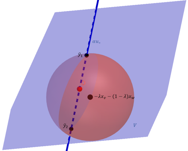
Figure 4.1. 3d representation of (4.9). The sphere $\mathcal{S}(\lambda)$ in red is centered in ${-(\lambda(x_{v})-(1-\lambda)x_{w})}$. $V$ is in light blue, while the line $\alpha y_{v}$ is in dark blue. $\mathcal{S}(\lambda)$ intersects $\alpha y_{v}$ in the points $\tilde{y}_{1}$ and $\tilde{y}_{2}$. $0$ is in red. The picture was built with the 3D calculator of Geogebra, [15].

Remark 3.

For $H=\mathbb{R}^{n}$, assumption $ii.$ of Theorem 11 is automatically satisfied if $m+1<n$. This assumption is close to $m+1\leq n$. For $H=\mathbb{R}^{n}$ and $m+1\leq n$, Theorem 11 can be considered a special case of Theorem 2.3 from [3].

Remark 4.

1. In 4.1, we provide a geometrical representation of the sets defined in (4.12), in the space of the variable $y\in\mathbb{R}^{3}$, with $m=1$ such that $m+1=2<n=3$. In $\mathbb{R}^{3}$, the above prove shows that the sphere $\mathcal{S}(\lambda)$ centered in ${-(\lambda(x_{v})+(1-\lambda)x_{w})}$ of radius ${\sqrt{\lambda\|x_{v}\|^{2}+(1-\lambda)\|x_{w}\|^{2}}}$, always intersects the line $\alpha u_{*}$ of parameter $\alpha$, where $u_{*}$ belongs to a basis of the vector space $V$. In fact,

   • the distance between $0$ and ${-(\lambda(x_{v})+(1-\lambda)x_{w})}$ is always less than the radius of $\mathcal{S}(\lambda)$ by (4.18),

   • the line $\alpha u_{*}$ passes through $0$.

2. Observe that the assumption $\bar{m}<n$ is important for the validity of the presented proof of Theorem 11 in finite dimensions. Otherwise, the only solution of the system (4.13) is $y=0$ which implies that it must be $\tilde{x}=\lambda x_{v}+(1-\lambda)x_{w}\in\mathcal{S}(\lambda)$, i.e. $\lambda x_{v}\perp(1-\lambda)x_{w}$ which can hardly be satisfied.

3. Under the assumption of Theorem 11, there could exist a component $i\in\{0,...,m\}$ such that $f_{i}(x):=\|x\|^{2}$ and a component $j\in\{0,...,m\}$ such that $f_{j}(x):=-\|x\|^{2}$.

   In this case, $\tilde{x}$ must satisfies

   $$\begin{cases}&\|\tilde{x}\|^{2}\leq\lambda\|x_{v}\|^{2}+(1-\lambda)\|x_{w}\|^{2}\\ &-\|\tilde{x}\|^{2}\leq-(\lambda\|x_{v}\|^{2}+(1-\lambda)\|x_{w}\|^{2})\end{cases}$$

   The above proves that, in order to complete the proof of Theorem 11, we cannot choose $\tilde{x}$ such that

   $$\|\tilde{x}\|^{2}\neq\lambda\|x_{v}\|^{2}+(1-\lambda)\|x_{w}\|^{2}$$

   This motivates our approach of looking for suitable $\tilde{x}$ from among elements of $\mathcal{S}(\lambda)$.

Theorem 11 allows us to prove that (KKT) conditions are necessary and sufficient optimality conditions for S-QCQP, as stated in the following theorem.

Theorem 12.

Consider S-QCQP and let the assumption of Theorem (11) be satisfied. Let Assumption 2 holds and $x^{*}$ be a global minimizer of S-QCQP. Then the Fritz-John conditions (3.8) are necessary for optimality. Moreover, if there exists a point $x_{0}\in H$ such that

$$f_{k}(x_{0})<0\ \ \ \forall\,k\in\{1,...,m\},$$

then, for a feasible $x^{*}$, the conditions (KKT) take the form: there exists a vector $(\gamma_{1},...,\gamma_{m})\in\mathbb{R}^{m}_{+}\backslash 0$ such that

$$\begin{split}&(i)\ \ \ 2a_{J}x^{*}+b_{J}+2\sum\limits_{k=1}^{m}2a_{k}x^{*}+b_{k}=0,\\ &(ii)\ \ \gamma_{k}f_{k}(x^{*})=0\ \ k\in\{1,...,m\},\\ &(iii)\ \ \ a_{J}+\sum\limits_{k=1}^{m}\gamma_{k}a_{k}\geq 0,\end{split}$$ (KKT)

are necessary and sufficient for global optimality of $x^{*}$.

Proof.

By Theorem 11, GIS is convex. We can apply Theorem 8 to complete the proof. $A_{J}+\sum\limits_{k=1}^{m}\gamma_{k}A_{k}$ can be rewritten as $(a_{J}+\sum\limits_{k=1}^{m}\gamma_{k}a_{k})I$ when Assumption 1 holds. Then, condition (iii) of (KKT) becomes $a_{J}+\sum\limits_{k=1}^{m}\gamma_{k}a_{k}\geq 0$ for S-QCQP.

∎

Remark 5.

Let $A:H\rightarrow H$ be a continuous linear operator. Let the corresponding quadratic form $\langle x,Ax\rangle$ be positive definite, i.e. there exists $\alpha>0$ such that, $\forall\,x\in H$, $\langle x,Ax\rangle\geq\alpha\|x\|^{2}$, see [14]. Then the function $\|\cdot\|_{A}:H\rightarrow\mathbb{R}_{+}$ defined as $\|x\|_{A}=\sqrt{\langle x,Ax\rangle}$ is a norm in $H$ (see [4], section 3.3.2). With this observation, the characterisation of Theorem 12 holds for scalar QCQP problems satisfying the following assumption.

Assumption 3.

Let $A:H\rightarrow H$ be a continuous linear operator such that $\langle x,Ax\rangle$ is positive definite. Let $A_{J},A_{k}$ $\forall\,k\in\{1,...,m\}$ be of the form $A_{J}=a_{J}A$, $A_{k}=a_{k}A$, where $a_{J},a_{k}\in\mathbb{R}$. Then, $A$ induce the norm $\|\cdot\|_{A}$.

Conditions for a positive quadratic form to be positive definite can be found in Theorem 10.1 of [14].

5. Conclusions

According to Theorem 8, the convexity of GIS and the Slater-type constraint qualification for a given QCQP suffice to characterize its global optimality in terms of KKT-type conditions. It is an open problem what is the largest class of QCQP problems for which such characterization holds true.

References

• [1] Moussa Barro, Ali Ouedraogo, and Sado Traore. Global optimality condition for quadratic optimization problems under data uncertainty. Positivity, 25(3):1027–1044, 2021.
• [2] Heinz H Bauschke and Patrick L Combettes. Convex Analysis and Monotone Operator Theory in Hilbert Spaces. Springer, 2017.
• [3] Amir Beck. On the convexity of a class of quadratic mappings and its application to the problem of finding the smallest ball enclosing a given intersection of balls. Journal of Global Optimization, 39(1):113–126, 2007.
• [4] J Frédéric Bonnans and Alexander Shapiro. Perturbation analysis of optimization problems. Springer Science & Business Media, 2013.
• [5] Samuel Burer and Dieter Vandenbussche. A finite branch-and-bound algorithm for nonconvex quadratic programming via semidefinite relaxations. Mathematical Programming, 113(2):259–282, 2008.
• [6] von Contino, Maximiliano, Guillermina Fongi, and Santiago Muro. Polyak’s theorem on hilbert spaces. Optimization, pages 1–15, 2022.
• [7] Frank Deutsch. Best approximation in inner product spaces, volume 7. Springer, 2001.
• [8] Vu Van Dong and Nguyen Nang Tam. On the solution existence of nonconvex quadratic programming problems in hilbert spaces. Acta Mathematica Vietnamica, 43(1):155–174, 2018.
• [9] AL Fradkov and VA Yakubovich. Thes-procedure and duality relations in nonconvex problems of quadratic programming. Vestn. LGU, Ser. Mat., Mekh., Astron,(1), pages 101–109, 1979.
• [10] Franco Giannessi. Constrained Optimization and Image Space Analysis: Volume 1: Separation of Sets and Optimality Conditions, volume 49. Springer Science & Business Media, 2006.
• [11] Gene H Golub, Per Christian Hansen, and Dianne P O’Leary. Tikhonov regularization and total least squares. SIAM journal on matrix analysis and applications, 21(1):185–194, 1999.
• [12] Jacek Gondzio and E Alper Yıldırım. Global solutions of nonconvex standard quadratic programs via mixed integer linear programming reformulations. Journal of Global Optimization, 81(2):293–321, 2021.
• [13] Sergei V Gusev and Andrey L Likhtarnikov. Kalman-popov-yakubovich lemma and the s-procedure: A historical essay. Automation and Remote Control, 67(11):1768–1810, 2006.
• [14] Magnus R Hestenes. Applications of the theory of quadratic forms in hilbert space to the calculus of variations. Pacific J. Math., 1(1):525–581, 1951.
• [15] Markus Hohenwarter. GeoGebra: Ein Softwaresystem für dynamische Geometrie und Algebra der Ebene. Master’s thesis, Paris Lodron University, Salzburg, Austria, February 2002. (In German.).
• [16] Richard B Holmes. Geometric functional analysis and its applications, volume 24. Springer Science & Business Media, 2012.
• [17] Seyedmohammadhossein Hosseinian, Dalila BMM Fontes, and Sergiy Butenko. A nonconvex quadratic optimization approach to the maximum edge weight clique problem. Journal of Global Optimization, 72:219–240, 2018.
• [18] Vaithilingam Jeyakumar, Gue Myung Lee, and Guoyin Y Li. Alternative theorems for quadratic inequality systems and global quadratic optimization. SIAM Journal on Optimization, 20(2):983–1001, 2009.
• [19] Vaithilingam Jeyakumar, Alex M Rubinov, and Zhi-You Wu. Non-convex quadratic minimization problems with quadratic constraints: global optimality conditions. Mathematical programming, 110(3):521–541, 2007.
• [20] Ching-pei Lee and Stephen J Wright. Inexact successive quadratic approximation for regularized optimization. Computational Optimization and Applications, 72:641–674, 2019.
• [21] Marco Locatelli and Fabio Schoen. Global optimization: theory, algorithms, and applications. SIAM, 2013.
• [22] Jaehyun Park and Stephen Boyd. General heuristics for nonconvex quadratically constrained quadratic programming. arXiv preprint arXiv:1703.07870, 2017.
• [23] Pablo A Parrilo, Grigoriy Blekherman, and Rekha R Thomas. Semidefinite optimization and convex algebraic geometry. SIAM Society for Industrial and Applied Mathematics., 2013.
• [24] Imre Pólik and Tamás Terlaky. A survey of the s-lemma. SIAM review, 49(3):371–418, 2007.
• [25] Ralph Tyrell Rockafellar. Convex analysis. In Convex analysis. Princeton university press, 2015.
• [26] M Ruiz Galán. A theorem of the alternative with an arbitrary number of inequalities and quadratic programming. Journal of Global Optimization, 69(2):427–442, 2017.
• [27] Marco Signoretto, Kristiaan Pelckmans, and Johan AK Suykens. Quadratically constrained quadratic programming for subspace selection in kernel regression estimation. In Artificial Neural Networks-ICANN 2008: 18th International Conference, Prague, Czech Republic, September 3-6, 2008, Proceedings, Part I 18, pages 175–184. Springer, 2008.
• [28] Mengmeng Song and Yong Xia. Calabi-polyak convexity theorem, yuan’s lemma and s-lemma: extensions and applications. Journal of Global Optimization, pages 1–14, 2022.
• [29] Petro I Stetsyuk, Tatiana E Romanova, and Guntram Scheithauer. On the global minimum in a balanced circular packing problem. Optimization Letters, 10(6):1347–1360, 2016.
• [30] Vu Van Dong. Optimality conditions for quadratic programming problems in hilbert spaces. Taiwanese Journal of Mathematics, 25(5):1073–1088, 2021.
• [31] Yong Xia, Shu Wang, and Ruey-Lin Sheu. S-lemma with equality and its applications. Mathematical Programming, 156:513–547, 2016.
• [32] Yong Xia, Meijia Yang, and Shu Wang. Chebyshev center of the intersection of balls: complexity, relaxation and approximation. Mathematical Programming, 187(1):287–315, 2021.
• [33] VA Yakubovich. Nonconvex optimization problem: The infinite-horizon linear-quadratic control problem with quadratic constraints. Systems & Control Letters, 19(1):13–22, 1992.