Improving Performance of Quantum Heat Engines by Free Evolution

Abstract

The efficiency of a quantum heat engine is maximum when the unitary strokes are adiabatic. On the other hand, this may not be always possible due to small energy gaps in the system, especially at the critical point where the gap vanishes. With the aim to achieve this adiabaticity, we modify one of the unitary strokes of the cycle by allowing the system to evolve freely with a particular Hamiltonian till a time so that the system reaches a less excited state. This will help in increasing the magnitude of the heat absorbed from the hot bath so that the work output and efficiency of the engine can be increased. We demonstrate this method using an integrable model and a non-integrable model as the working medium. In the case of a two spin system, the optimal value for the time till which the system needs to be freely evolved is calculated analytically in the adiabatic limit. The results show that implementing this modified stroke significantly improves the work output and efficiency of the engine, especially when it crosses the critical point.

I Introduction

Studies on experimental realization of various quantum devices where the working medium is described by a quantum Hamiltonian, have given a large push to an already active area of research Mukherjee and Divakaran (2021); Bhattacharjee and Dutta (2021); Myers et al. (2022). These devices include quantum refrigerators Abah and Lutz (2016); Maslennikov et al. (2019), quantum batteries Le et al. (2018); Bhattacharjee and Dutta (2021), quantum transistors Gupt et al. (2022) with quantum heat engines (QHE) Gemmer et al. (2009); Quan et al. (2007) receiving maximum attention recently. The QHEs are being explored experimentally using a variety of platforms namely, trapped ions or ultracold atoms Roßnagel et al. (2016); von Lindenfels et al. (2019), optical cavities Schreiber et al. (2015), using NMR techniques Peterson et al. (2019), nitrogen vacancy centres in diamond Klatzow et al. (2019), etc. Theoretical studies on QHE first concentrated on few body systems such as single spin systems Feldmann and Kosloff (2000); Gelbwaser-Klimovsky et al. (2013), two spin systems Thomas and Johal (2011); Campisi et al. (2015), and harmonic oscillators Kosloff and Rezek (2017); Rezek and Kosloff (2006). Recently, the focus has shifted to many body systems as working media (WM), mainly to understand the effect of various interactions present in the many body WM. This included effects like collective cooperative effects Niedenzu and Kurizki (2018); Chen and del Campo (2019); Jaramillo et al. (2016), super-radiance Hardal and Müstecaplıoğlu (2015), many body localization Yunger Halpern et al. (2019), and phase transitions Campisi and Fazio (2016); Fogarty and Busch (2020); Piccitto et al. (2022); Ma et al. (2017). The performance of these engines are quantified using parameters like efficiency defined as the ratio of work done by the engine to the heat absorbed, and power defined as the ratio of work done to the total cycle time.

Phase transitions in quantum heat engines have been studied in Refs. Campisi and Fazio (2016); Fogarty and Busch (2020); Piccitto et al. (2022); Ma et al. (2017). In Ref. Revathy et al. (2020), we reported the universality in the finite time dynamics of quantum heat engines using critical working medium, where we also showed that crossing the critical point (CP) leads to generation of excitations which are detrimental to the performance of the engines. These excitations can be reduced if the CP is crossed slowly, which essentially implies increasing the cycle time of the engine. But this results in vanishing power output as it is inversely proportional to the cycle time. In order to increase the efficiency of the engine without sacrificing the power output, many control techniques have been put forward, the prominent one being the shortcuts to adiabaticity (STA) del Campo et al. (2012); Kolodrubetz et al. (2017); Guéry-Odelin et al. (2019). STA has been highly instrumental in improving the performance of quantum machines Hartmann et al. (2020); del Campo et al. (2014); Deng et al. (2013); Beau et al. (2016); Sels and Polkovnikov (2017); Abah and Lutz (2018). At the same time it requires additional control Hamiltonian which may involve long range interactions as well del Campo et al. (2012); Kolodrubetz et al. (2017), making the process complicated.

In Ref. Revathy et al. (2022), bath engineered quantum engine was proposed to overcome the effects of the excitations by removing those modes during the non-unitary strokes which were reducing the work done. On the other hand, in this paper, we propose a simple way to improve the performance of the engine by modifying the unitary stroke where the system is freely evolved with a different Hamiltonian for a certain time. We illustrate the idea of free evolution using an integrable and a non-integrable WM and show that free evolution indeed aids in better performance of engines compared to normal finite time engines. The outline of the paper is as follows: In Sec. II, the conventional four stroke quantum Otto cycle is discussed followed by the proposed modification. Sec. III discusses the transverse Ising model whereas the antiferromagnetic transverse Ising model with longitudinal field as the WM is discussed in Sec. IV. Finally we conclude in Sec. V.

II Quantum Otto Cycle and free evolution

The working medium (WM) of the many body quantum Otto cycle is described by the Hamiltonian

$$H(t)=H_{0}+\lambda(t)H_{1},$$ (1)

where $\lambda$ is the time dependent parameter that can be varied. The usual four stroke quantum Otto cycle consists of two unitary strokes and two non-unitary strokes as described below.

• Non-unitary stroke A $\rightarrow$ B: The WM with parameter $\lambda_{1}$ is connected to the hot bath which is at a temperature $T_{H}$ till a time $\tau_{H}$ so that it reaches the thermal state at B given by

  $$\rho_{B}=\frac{e^{-\beta_{H}H(\lambda_{1})}}{Z(\lambda_{1})},$$ (2)

  where $\beta_{H}=\frac{1}{k_{B}T_{H}}$, (we have taken $k_{B}=1$) and $Z$ is the partition function ($Z=\text{Tr}(e^{-\beta_{H}H(\lambda_{1})}))$. Let us represent the energy exchanged in this stroke by $\mathcal{Q}_{in}$.

• Unitary stroke B $\rightarrow$ C: The WM is decoupled from the hot bath and $\lambda$ is changed from $\lambda_{1}$ to $\lambda_{2}$ with a speed $1/\tau_{1}$.

  This unitary evolution is described by the von-Neumann equation of motion:

  $$\frac{d\rho}{dt}=-i[H,\rho].$$ (3)

• Non-unitary stroke C $\rightarrow$ D: The WM with $\lambda_{2}$ is now connected to the cold bath which is at a temperature $T_{C}$ till $\tau_{C}$ when it reaches the corresponding thermal state at D

  $$\rho_{D}=\frac{e^{-\beta_{C}H(\lambda_{2})}}{Z(\lambda_{2})},$$ (4)

  where $\beta_{C}=\frac{1}{k_{B}T_{C}}$.

  The energy exchanged in this stroke is represented by $\mathcal{Q}_{out}$.

• Unitary stroke D $\rightarrow$ A: After decoupling from the cold bath, the parameter is changed back to $\lambda_{1}$ from $\lambda_{2}$ with a speed $1/\tau_{2}$.

  These are the strokes of a conventional four stroke quantum Otto cycle. The energies at the end of each stroke $i$ is calculated using

  $$\mathcal{E}_{i}=\text{Tr}(H_{i}\rho_{i})$$ (5)

  with $i=\bf{A,B,C,D}$, $H_{i}$ is the Hamiltonian at $i$ and $\rho_{i}$ is the corresponding density matrix. The sign convention followed in this paper is as follows: the amount of energy absorbed by the WM ($\mathcal{Q}_{in}$) is taken to be positive whereas energy released by the WM ($\mathcal{Q}_{out}$) is taken to be negative. These energies can be calculated as follows :

  $$\mathcal{Q}_{in} = \mathcal{E}_{B}-\mathcal{E}_{A}$$ (6)

  $$\mathcal{Q}_{out} = \mathcal{E}_{D}-\mathcal{E}_{C}.$$ (7)

  The output work is $\mathcal{W}=-(\mathcal{Q}_{in}+\mathcal{Q}_{out})$. The quantum Otto cycle works as an engine if $\mathcal{Q}_{in}>0,\mathcal{Q}_{out}<0,\mathcal{W}<0$. The quantities of interest which characterize its performance are efficiency and the power output defined as

  $$\eta = -\frac{\mathcal{W}}{\mathcal{Q}_{in}}$$ (8)

  $$\mathcal{P} = \frac{\mathcal{W}}{\tau_{\text{total}}},$$ (9)

  where $\tau_{\text{total}}=\tau_{1}+\tau_{2}+\tau_{H}+\tau_{C}$.

  Let us now outline the modification proposed during the unitary stroke D $\rightarrow$ A, which will help in improving the performance of the engine.

  We modify the unitary stroke D $\rightarrow$ A by including free evolution for a particular time after the usual unitary evolution, see Fig. 1. As discussed, we shall show that this modification will improve both, the efficiency as well as the power of the engine. The exact protocol that we adopt is as follows :

  At D the WM is decoupled from the cold bath and $\lambda_{2}$ is changed back to $\lambda_{1}$ with a time dependence proportional to $t/\tau_{2}$ such that it reaches ${\mathbf{A^{\prime}}}$. At ${\mathbf{A^{\prime}}}$, $\lambda_{1}$ is switched off and the system is allowed to evolve freely using $H_{0}$ for a time $\tau_{k}$. The parameter $\lambda$ is again switched back to $\lambda_{1}$ at A after time $\tau_{k}$. The genesis of this idea comes from the fact that the unitary evolution from D to ${\mathbf{A^{\prime}}}$ will result in a state that is excited at ${\mathbf{A^{\prime}}}$ due to the non-adiabatic dynamics. Thus, the success of this modification strongly depends on whether $H_{0}$ is able to take the system to a lower energy state at ${\mathbf{A}}$. As we shall show below using examples, this is indeed possible. The WM is then connected to the hot bath in the non-unitary stroke A $\rightarrow$ B after which the other strokes are followed.

Figure 1: Schematic diagram of the modified quantum Otto cycle. At D the system is evolved to ${\mathbf{A^{\prime}}}$ with a linear time dependence. At ${\mathbf{A^{\prime}}}$, $\lambda_{1}$ is switched off and the system freely evolves with $H_{0}$ for a time $\tau_{k}$ to reach A where $\lambda_{1}$ is switched on.

In the following sections we implement these ideas into the quantum Otto cycle using an integrable as well as a non-integrable WM.

III Integrable Model as WM

Let us first consider the widely studied integrable model, the transverse field Ising model as the working medium. The Hamiltonian is given by

$$H=-J\sum_{n}\sigma_{n}^{z}\sigma_{n+1}^{z}-h(t)\sum_{n}\sigma_{n}^{x}$$ (10)

with $H_{0}=-J\sum_{n}\sigma_{n}^{z}\sigma_{n+1}^{z}$ and $H_{1}=-\sum_{n}\sigma_{n}^{x}$. Here, $\sigma_{n}^{\mu}$ with $\mu=x,y,z$ are the Pauli matrices at site $n$, $J$ is the nearest neighbour interaction strength and $h(t)$ is the transverse field which is the parameter $\lambda$ for TIM. The model shows quantum phase transition from the paramagnetic state ($h>>J$) to the ferromagnetic state ($h<<J$) with the quantum critical point occurring at $h=\pm J$ Lieb et al. (1961); Pfeuty (1970); Bunder and McKenzie (1999). The relaxation time diverges at the critical point. As a result, there will be excitations generated no matter how slow the parameter $h$ is varied, if the unitary strokes involve crossing the critical point Sachdev (2011); Dutta et al. (2015); Polkovnikov et al. (2011). For numerical calculations, we set $J=1$ and use periodic boundary conditions.

We now need to select a protocol to vary $h$ from $h_{1}$ to $h_{2}$ during the unitary strokes. The driving protocol for the B to C stroke is chosen to be

$$h(t)=h_{1}+(h_{2}-h_{1})\frac{t}{\tau_{1}},\hskip 14.22636pt0<t<\tau_{1}.$$ (11)

We have taken $h_{1}>>J$ and $h_{2}<h_{1}$. In the case of the freely evolved engine, once the system reaches the thermal state at D with $h=h_{2}$ and $T=T_{C}$, it is decoupled from the cold bath after which the transverse field is changed from $h_{2}$ to $h_{1}$ to reach ${\mathbf{A^{\prime}}}$ following

$$h(t)=h_{2}+(h_{1}-h_{2})\frac{(t-a)}{\tau_{2}},\hskip 14.22636pta<t<a+\tau_{2},$$ (12)

where $a=\tau_{C}+\tau_{1}$. At ${\mathbf{A^{\prime}}}$, the transverse field is switched off and the WM is allowed to evolve freely with $H_{0}$ till a time $\tau_{k}$. The transverse field is switched back to $h_{1}$ at $\tau_{k}$ which corresponds to point A in the Otto cycle after which it is connected to the hot bath at $T_{H}$, and the cycle repeats. We first plot the output work of the engine as a function of $\tau_{k}$ for $L=2$ and $L=10$ in Fig.(2). It is evident from Fig.(2) that for specific ranges of $\tau_{k}$ values, the output work of the freely evolved engine reaches a more negative value compared to that of normal finite time engines. Clearly, the magnitude of the work output by an engine is maximum when $\mathcal{E}_{A}$ is the minimum and that happens for optimal values of $\tau_{k}$. Identifying the optimal value of $\tau_{k}$ is important since it decides how much the work output can be increased which is same as how much the energy at A can be reduced. To get a better understanding of this optimal $\tau_{k}$, below we calculate $\tau_{k}$ for a two spin system analytically in the adiabatic limit.

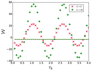
Figure 2: $\mathcal{W}$ as a function of $\tau_{k}$ for different system sizes for TIM. The data points correspond to freely evolved engines and the dashed line and the continuous line correspond to normal finite time engines of $L=2$ and $L=10$ respectively. The parameters are $h_{1}=10,h_{2}=0.2,T_{H}=100,T_{C}=0.001,\tau_{1}=0.1,\tau_{2}=0.1.$ The $\tau_{k}$ at which the maximum work is done by the engine, is also seen to be system size independent.

III.1 Two spin case

For a two spin system, the value of $\tau_{k}$ can be derived analytically in the adiabatic limit. The Hamiltonian for a two spin system at D in the $z$ basis with periodic boundary conditions is given by

$$H_{D}=\begin{bmatrix}-2J&-h_{2}&-h_{2}&0\\ -h_{2}&2J&0&-h_{2}\\ -h_{2}&0&2J&-h_{2}\\ 0&-h_{2}&-h_{2}&-2J\end{bmatrix},$$ (13)

with eigenenergies $\epsilon_{1},\epsilon_{2},\epsilon_{3},\epsilon_{4}$. Since the WM is in the thermal state corresponding to $T_{C}$ at D, the density matrix in the eigenbasis can be written as

$$\rho_{D}=\begin{bmatrix}\frac{e^{-\beta_{C}\epsilon_{1}}}{Z}&0&0&0\\ 0&\frac{e^{-\beta_{C}\epsilon_{2}}}{Z}&0&0\\ 0&0&\frac{e^{-\beta_{C}\epsilon_{3}}}{Z}&0\\ 0&0&0&\frac{e^{-\beta_{C}\epsilon_{4}}}{Z}\end{bmatrix},$$ (14)

where $\beta_{C}=\frac{1}{T_{C}}$ with $k_{B}=1$. Considering adiabatic evolution from D $\rightarrow$ ${\mathbf{A^{\prime}}}$ which corresponds to a large $\tau_{2}$, we can write $\rho_{D}=\rho_{A^{\prime}}$ in their respective eigenbasis. The energy at ${\mathbf{A^{\prime}}}$ can be calculated as

$$\mathcal{E}_{A^{\prime}} = \text{Tr}(H_{A}{{}^{\prime}}\rho_{A}{{}^{\prime}})$$ (15)

$$= -4h_{1}\alpha-\frac{4J^{2}\alpha}{h_{1}}+4J\delta$$ (16)

with

$$\alpha = \frac{h_{1}\sinh\left(\frac{2\sqrt{h_{2}^{2}+J^{2}}}{T_{C}}\right)}{2\sqrt{h_{1}^{2}+J^{2}}\left(\cosh\frac{2J}{T_{C}}+\cosh\frac{2\sqrt{h_{2}^{2}+J^{2}}}{T_{C}}\right)},$$ (17)

$$\delta = \frac{-\sinh(\frac{2J}{T_{C}})}{2\left(\cosh\frac{2J}{T_{C}}+\cosh\frac{2\sqrt{h_{2}^{2}+J^{2}}}{T_{C}}\right)}.$$ (18)

We now evolve $\rho_{A}{{}^{\prime}}$ with $U=\exp(-i(-J\sigma_{i}^{z}\sigma_{i+1}^{z})t)$ up to $\tau_{k}$ to reach A so that the energy at A takes the form

$$\mathcal{E}_{A}=-4h_{1}\alpha\cos(4J\tau_{k})-\frac{4J^{2}\alpha}{h_{1}}\cos(4h_{1})$$

$$+4J\delta-4J\alpha\sin(4h_{1})\sin(4J\tau_{k}),$$ (19)

where $H_{A^{\prime}}=H_{A}$.

Since we aim to obtain the $\tau_{k}$ for which $\mathcal{E}_{A}$ is minimum, we optimize $\mathcal{E}_{A}$ with respect to $\tau_{k}$ to get

$$\tan(4J\tau_{k})=\frac{J}{h_{1}}\sin(4h_{1})$$ (20)

so that minimum $\mathcal{E}_{A}$ occurs at $\tau_{k}^{opt}=n\pi/4$ with $n=0,2,4,..$. It is to be noted that adiabatic evolution requires infinite time which results in zero output power. Realistic engines are finite time engines which work with finite $\tau_{1}$ and $\tau_{2}$. Therefore, the optimal value of $\tau_{k}$ obtained through Eq. (20) may not be the optimal value for a finite time engine, especially when $h_{2}$ is less than the critical value of the field so that the critical point is crossed during the unitary strokes. We plot $\mathcal{E}_{A}$ obtained in Eq. (III.1) with $\tau_{k}$ and compare with finite time engines in Fig. (3), which shows that $\tau_{k}^{opt}$ for an adiabatic evolution occurs at $\tau_{k}=0$ whereas for the finite engines with $\tau_{1}=\tau_{2}=0.1$, this happens at $\tau_{k}=0.3$ for the given parameters. Clearly, after an adiabatic evolution, the system starts from a lower energy state whereas for finite time evolution, the system can reach a lower energy state due to free evolution. As evident from Fig. (3), when $\tau_{1},\tau_{2}$ increases to the value $1$, we see that the minima of $\mathcal{E}_{A}$ shifts closer and closer to the adiabatic minima. It is to be noted that $\tau_{k}^{opt}$ is different for different $h_{2}$ unless in the adiabatic limit (see Eq. (20)).

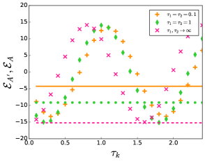
Figure 3: $\mathcal{E}_{A}$ as a function of $\tau_{k}$ for $L=2$ comparing adiabatic engine with finite time engines. Here, the marker points correspond to $\mathcal{E}_{A}$ whereas the continuous, dotted and dashed line correspond to $\mathcal{E}_{A^{\prime}}$ for $\tau_{1}=\tau_{2}=0.1$, $\tau_{1},\tau_{2}=1$ and $\tau_{1},\tau_{2}\rightarrow\infty$, respectively. The parameters are $L=2,h_{1}=10,h_{2}=0.1,T_{H}=100,T_{C}=0.01$.

We also stress here that the adiabatic evolution is the best possible way of evolution by which no excitations occur in the system. Therefore, if ${\mathbf{A^{\prime}}}$ is reached after an adiabatic evolution, no free evolution can take the system to a lower energy state at A as compared to ${\mathbf{A^{\prime}}}$. On the other hand, if ${\mathbf{A^{\prime}}}$ is reached in finite time, there is a possibility of taking the system to a lower energy state at A through free evolution.

The optimal $\tau_{k}$ value obtained for the two spin case is the same for larger system sizes as also seen in Fig.(2). In appendix A, we analytically calculate the value of optimal $\tau_{k}$ for different system sizes in the adiabatic limit and show that this $\tau_{k}^{opt}$ is indeed independent of system size.

We now study the variation of output work and efficiency for the free evolved engine with $\tau_{k}$ set to $\tau_{k}^{opt}$ and compare it with usual finite time engines with same $\tau_{1}$ and $\tau_{2}$. Fig. (4) shows the output work as a function of $h_{2}$ for different system sizes. In the engines where $h_{2}$ is close to the critical point or below it, we see that the additional free evolution of the engine improves the work output of the engine to a great extent for all system sizes. Similar behavior is also seen in the efficiency plot (inset of Fig.(4)). This is due to the fact that the the energies at ${\mathbf{A^{\prime}}}$ and A follow the inequality $\mathcal{E}_{A}<\mathcal{E}_{A^{\prime}}$ resulting to an increase in the magnitude of $\mathcal{Q}_{in}$ which further reflects in the improved output work and efficiency.

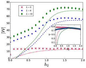
Figure 4: $\mathcal{|W|}$ as a function of $h_{2}$ for different system sizes of TIM. The data points correspond to freely evolved engines and the dotted, dashed and continuous line correspond to the work done by the finite time engines of system sizes $L=2$, $L=8$ and $L=10$, respectively. Inset: $\eta$ as a function of $h_{2}$ with the same legend as in the main figure. The parameters are $h_{1}=10,T_{H}=100,T_{C}=0.001,\tau_{1}=0.1,\tau_{2}=0.1.$

Adiabatic evolution ($\tau_{1},\tau_{2}\rightarrow\infty$) leads to highly efficient engines but at the cost of output power. As can be easily verified, increasing $\tau_{1}$ and $\tau_{2}$ enables finite time engines to reach adiabatic efficiency value $\eta_{adia}$. But this clearly reduces the output power due to large values of $\tau_{1}$ and $\tau_{2}$. In contrast, the free evolved engines have high efficiency closer to $\eta_{adia}$ at small values of $\tau_{1}$ and $\tau_{2}$ (with free evolved $\tau_{k}^{opt}$) along with finite power. This can be seen from the inset of Fig.(5). Even with smaller values of $\tau_{1}$ , $\tau_{2}$ and $\tau_{k}=\tau_{k}^{opt}$, we see that the efficiency as well as the power improves in case of the free evolved engines compared to normal finite time engines with larger $\tau_{1}$ and $\tau_{2}$. In other words, we get better efficiency and output power with smaller total cycle time ($\tau_{1}+\tau_{2}+\tau_{H}+\tau_{C}+\tau_{k}$) compared to usual finite time engines where decreasing cycle time will lead to increase in output power but with reduced efficiency.

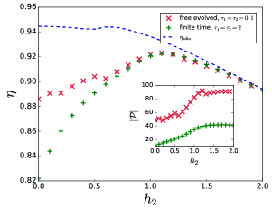
Figure 5: $\eta$ as a function of $h_{2}$ for $L=10$ TIM. Inset: $\mathcal{|P|}$ as a function of $h_{2}$. The parameters are $h_{1}=20,T_{H}=1000,T_{C}=0.001$. We have set $\tau_{H}+\tau_{C}=0.2$. The values of $\tau_{1}$ and $\tau_{2}$ for the freely evolved engine is intentionally chosen to be lesser than that of normal finite time engine to highlight the advantage of free evolution. For the freely evolved engine, optimal $\tau_{k}$ value is $h_{2}$ dependent.

We also extend the technique of free evolution to the momentum ($k$) space which allows us to go to higher system sizes. The Hamiltonian in Eq. (10) when written in $k$ space takes the form

$$H=\sum_{k>0}\psi_{k}^{\dagger}H_{k}\psi_{k}$$ (21)

with $\psi_{k}^{\dagger}=(c_{k}^{\dagger},c_{-k})$ and

$$H_{k}=\begin{bmatrix}2(h(t)+\cos k)&0&0&2\sin k\\ 0&0&0&0\\ 0&0&0&0\\ 2\sin k&0&0&-2(h(t)+\cos k)\end{bmatrix}.$$ (22)

The unitary dynamics that is undergone in the B to C and D to A strokes is described by the von-Neumann equation and the density matrix at B and D for each $k$ mode will be the thermal state corresponding to $T_{H}$ and $T_{C}$ respectively, as given in Ref. Revathy et al. (2022). For the free evolution, the density matrix at A for each mode can be written as

$$\rho_{k}^{A}=U_{k}\rho_{k}^{A^{\prime}}U_{k}^{\dagger},$$ (23)

with $U_{k}=\exp(-iH^{\prime}_{k}\tau_{k})$ and $H^{\prime}_{k}=H_{k}$ with $h(t)=0$. As discussed before, the $\tau_{k}^{opt}$ is independent of system size which has been verified numerically in momentum space. This further helps in extending the technique to larger system sizes.

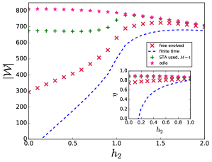
Figure 6: $\mathcal{|W|}$ as a function of $h_{2}$ for $L=100$ TIM. The parameters are $h_{1}=10,T_{H}=100,T_{C}=0.001,\tau_{1}=0.1,\tau_{2}=0.1$. We have set $\tau_{H}+\tau_{C}=0.2$. Inset: $\eta$ as a function of $h_{2}$ with the same legend as in the main figure. For the freely evolved engine, optimal $\tau_{k}$ value is $h_{2}$ dependent. The control Hamiltonian for STA is truncated to $M$ body terms with $M=4$ del Campo et al. (2012).

In Fig. 6, we plot the work output and efficiency (in the inset) by the free evolved engines as a function of $h_{2}$ for $L=100$ and compare it with normal finite time engine, finite time engine using STA, and adiabatic engine. As expected, the free evolved engine performs better than the finite time engine without any control. On the contrary, its performance is lower when compared with finite time engines using STA. But we emphasize here the simplicity of implementing this protocol as compared to STA.

We further extend the technique of free evolution to a non-integrable model in the next section and show the effectiveness of this protocol.

IV Non integrable Model as WM

In this section we use a non-integrable model, the antiferromagnetic transverse Ising model with longitudinal field (LTIM) to demonstrate the freely evolved engine. The Hamiltonian is given by Sharma et al. (2015); Bonfim et al. (2019)

$$H=J\sum_{n}\sigma_{n}^{z}\sigma_{n+1}^{z}-h(t)\sum_{n}\sigma_{n}^{x}-B_{z}\sum_{n}\sigma_{n}^{z},$$ (24)

where $J$ is the antiferromagnetic interaction , $B_{z}$ is the longitudinal field and $h$ is the time dependent transverse field which is varied as given in Eqs. (11) and (12) during the unitary strokes.

In the case of LTIM, $H_{0}=J\sum_{n}\sigma_{n}^{z}\sigma_{n+1}^{z}-B_{z}\sum_{n}\sigma_{n}^{z}$ and $H_{1}=-h(t)\sum_{n}\sigma_{n}^{x}$ so that $h$ is switched off to zero between ${\mathbf{A^{\prime}}}$ and A for a time $\tau_{k}$. At A, $h(t)$ is again switched back to $h_{1}$ and the cycle repeats.

In Fig.(7), the work output of the free evolved engine as well as normal finite time engines is plotted as a function of $h_{2}$ for different system sizes of LTIM. Similar to the case of TIM, we observe a significant improvement in the work output of the free evolved engine, especially for small values of $h_{2}$ where the energy gaps are small. As mentioned before, here also $\tau_{k}^{opt}$ is different for different $h_{2}$. The improvement in the performance of the engine is also visible in terms of its efficiency, as shown in the inset of Fig. (7).

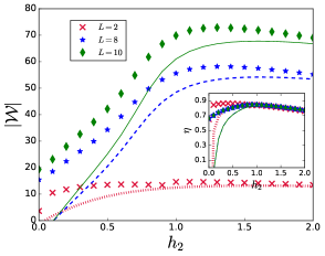
Figure 7: $\mathcal{|W|}$ as a function of $h_{2}$ for different system sizes in case of LTIM. The data points correspond to freely evolved engines and the dotted, dashed and continuous line correspond to the work done by the finite time engines of system sizes $L=2$, $L=8$ and $L=10$, respectively. The parameters are $B_{z}=1,h_{1}=10,T_{H}=100,T_{C}=0.001,\tau_{1}=0.1,\tau_{2}=0.1$. Inset: $\eta$ as function of $h_{2}$ with the same legend as in the main figure.

The $\tau_{k}^{opt}$ value for different system sizes can be found out analytically in the adiabatic limit and is presented in Appendix B. For the case of LTIM also, the $\tau_{k}^{opt}$ is found to be system size independent.

V Conclusions

Through this work, we propose a simple and effective way to improve the work output and efficiency of a quantum Otto engine which uses a quantum substance as the working medium. The excitations produced during the operation of the engine causes reduction in its performance. This can be avoided using the simple method that we propose. We modify one of the unitary strokes by first letting it undergo the usual unitary dynamics and then doing a free evolution after switching off one of the terms of the original Hamiltonian. Our results using the integrable as well as the non-integrable model shows that this method helps significantly in improving the performance of the engine. Unlike the conventional techniques such as shortcuts to adiabaticity or the bath engineering techniques which may involve some additional cost for their implementation, our method just requires switching off of the time dependent parameter in the Hamiltonian and evolving the system freely for a specific time making it easier to implement without any additional costs.

We also highlight the fact that the proposed protocol will be useful only if the energy at A is less than the energy at ${\mathbf{A^{\prime}}}$ after free evolution for time $\tau_{k}$. For this, choosing the correct $\tau_{k}^{opt}$ is very important. In this work, we have demonstrated the power of free evolution technique by switching off some of the terms of the Hamiltonian such that the free evolution is in presence of the remaining terms in the original Hamiltonian. We do acknowledge the fact that this may not be the best protocol. In fact if the target state at A is known beforehand, the free evolution Hamiltonian which need not be any of the terms in the original Hamiltonian, can be chosen wisely so that the system is indeed taken as close to the target state as possible.

Experimental implementation of this protocol is also straightforward since it only involves tuning of the transverse field or some terms already present in the Hamiltonian. This makes the technique easy to implement.

Appendix A Finding $\tau_{k}^{opt}$ for different system sizes : TIM

We find an analytical estimate of the optimal $\tau_{k}$ value for different system sizes, in the adiabatic limit. Consider the cold bath temperature to be zero so that the system reaches the ground state at D. Let the system evolves adiabatically from D $\rightarrow$ $\mathbf{{A^{\prime}}}$ which takes it to the ground state at ${\mathbf{A^{\prime}}}$. Since $h_{1}>>1$, the state at ${A^{\prime}}$ can be written as

$$|\psi\rangle_{A^{\prime}}=\otimes_{L}|\rightarrow\rangle$$ (25)

with all spins aligned along the $x$- direction. The system is then allowed to evolve freely with $H_{0}$ with an evolution operator $U$ given by

$$U = \exp(-i(-J\sum_{n}\sigma_{n}^{z}\sigma_{n+1}^{z})\tau_{k})$$ (26)

$$= \displaystyle\prod_{n}\left(\cos(J\tau_{k})+i\sin(J\tau_{k})\sigma_{n}^{z}\sigma_{n+1}^{z}\right),$$ (27)

so that the state reached at A for a two spin system is

$$|\psi\rangle_{A}=\cos(2J\tau_{k})|\rightarrow\rightarrow\rangle+i\sin(2J\tau_{k})|\leftarrow\leftarrow\rangle.$$ (28)

Similarly, the state at A for a 4-spin system is

$$|\psi\rangle_{A} = \left(\cos^{4}(J\tau_{k})+\sin^{4}(J\tau_{k})\right)|\rightarrow\rightarrow\rightarrow\rightarrow\rangle$$ (29)

$$-2\sin^{2}(J\tau)\cos^{2}(J\tau)|\leftarrow\leftarrow\leftarrow\leftarrow\rangle$$

$$-2\sin^{2}(J\tau)\cos^{2}(J\tau)(|\leftarrow\rightarrow\leftarrow\rightarrow\rangle+|\rightarrow\leftarrow\rightarrow\leftarrow\rangle)$$

$$(i\sin(J\tau)\cos^{3}(J\tau)-i\sin^{3}(J\tau)\cos(J\tau))$$

$$(|\rightarrow\rightarrow\leftarrow\leftarrow\rangle+|\leftarrow\leftarrow\rightarrow\rightarrow\rangle$$

$$+|\rightarrow\leftarrow\leftarrow\rightarrow\rangle+|\leftarrow\rightarrow\rightarrow\leftarrow\rangle).$$

Since the ground state is all spins along the $x$- direction, the probability for the system to be in its ground state at A is given by $\cos^{2}(2J\tau_{k})$ for $L=2$ and $(\cos^{4}(J\tau_{k})+\sin^{4}(J\tau_{k}))^{2}$ for $L=4$. Our goal is to take the system to the lowest possible energy state at A. Therefore we maximize the probability for the system to be in the ground state, to obtain the optimal $\tau_{k}$ at $\tau_{k}^{opt}=n\pi/4J$ with $n=0,2,4,..$ for both $L=2$ and $L=4$. We have checked numerically and found it to be true for larger system sizes as well and thus the $\tau_{k}^{opt}$ is the same for all $L$. A general expression for the probability of a system of size $L$ to be in its ground state is given by $|a|^{2}$ where $a=\cos(J\tau_{k})^{L}+(i\sin(J\tau_{k}))^{L}$, which we have also verified numerically.

Appendix B Finding $\tau_{k}^{opt}$ for LTIM

We follow the same procedure as in the case of TIM (given in Appendix A) to show that the optimal value of $\tau_{k}$ is the same for all system sizes of LTIM as well. For a two spin system, the probability of the system to be in the ground state after adiabatic evolution at A is given by $\cos(B_{z}\tau_{k})^{4}\cos(2J\tau_{k})^{2}+\sin(2J\tau_{k})^{2}\sin(B_{z}\tau_{k})^{4}$ and that for $L=4$ is given by $(\cos(B_{z}\tau_{k})^{4}(\cos(J\tau_{k})^{4}+\sin(J\tau_{k})^{4})-2\sin(J\tau_{k})^{2}\cos(J\tau_{k})^{2}\sin(B_{z}\tau_{k})^{4})^{2}$. The maxima for these functions when $B_{z}$ and $J$ is set to unity, occur at $\tau_{k}^{opt}=n\pi$ with $n=0,1,2..$ which gives the $\tau_{k}^{opt}$ values. This is verified in Fig.(8) where we plot $\mathcal{E}_{A^{\prime}}$ and $\mathcal{E}_{A}$ as a function of $\tau_{k}$ for different system sizes. It is observed that even in the diabatic limit ($\tau_{2}=0.1$), the minimum $\mathcal{E}_{A}$ occurs at the same $\tau_{k}$ for both $L=2$ and $L=10$, implying that $\tau_{k}^{opt}$ indeed is system size independent.

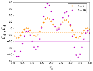
Figure 8: $\mathcal{E}_{A}$ as a function of $\tau_{k}$ for different system sizes. Here dashed line and continuous line represent $\mathcal{E}_{A^{\prime}}$ for $L=2$ and $L=10$, respectively. The parameters are $B_{z}=1,h_{1}=10,h_{2}=0.1,T_{H}=100,T_{C}=0.001,\tau_{1}=0.1,\tau_{2}=0.1$.

References

- Mukherjee and Divakaran (2021) V. Mukherjee and U. Divakaran, Journal of Physics: Condensed Matter 33, 454001 (2021).
- Bhattacharjee and Dutta (2021) S. Bhattacharjee and A. Dutta, The European Physical Journal B 94, 239 (2021).
- Myers et al. (2022) N. M. Myers, O. Abah, and S. Deffner, AVS Quantum Science 4, 027101 (2022), https://doi.org/10.1116/5.0083192 .
- Abah and Lutz (2016) O. Abah and E. Lutz, Europhysics Letters 113, 60002 (2016).
- Maslennikov et al. (2019) G. Maslennikov, S. Ding, R. Hablützel, J. Gan, A. Roulet, S. Nimmrichter, J. Dai, V. Scarani, and D. Matsukevich, Nature Communications 10, 202 (2019).
- Le et al. (2018) T. P. Le, J. Levinsen, K. Modi, M. M. Parish, and F. A. Pollock, Phys. Rev. A 97, 022106 (2018).
- Gupt et al. (2022) N. Gupt, S. Bhattacharyya, B. Das, S. Datta, V. Mukherjee, and A. Ghosh, Phys. Rev. E 106, 024110 (2022).
- Gemmer et al. (2009) J. Gemmer, M. Michel, and G. Mahler, Quantum thermodynamics: Emergence of thermodynamic behavior within composite quantum systems, Vol. 784 (Springer, 2009).
- Quan et al. (2007) H. T. Quan, Y.-x. Liu, C. P. Sun, and F. Nori, Phys. Rev. E 76, 031105 (2007).
- Roßnagel et al. (2016) J. Roßnagel, S. T. Dawkins, K. N. Tolazzi, O. Abah, E. Lutz, F. Schmidt-Kaler, and K. Singer, Science 352, 325 (2016).
- von Lindenfels et al. (2019) D. von Lindenfels, O. Gräb, C. T. Schmiegelow, V. Kaushal, J. Schulz, M. T. Mitchison, J. Goold, F. Schmidt-Kaler, and U. G. Poschinger, Phys. Rev. Lett. 123, 080602 (2019).
- Schreiber et al. (2015) M. Schreiber, S. S. Hodgman, P. Bordia, H. P. Lüschen, M. H. Fischer, R. Vosk, E. Altman, U. Schneider, and I. Bloch, Science 349, 842 (2015).
- Peterson et al. (2019) J. P. S. Peterson, T. B. Batalhão, M. Herrera, A. M. Souza, R. S. Sarthour, I. S. Oliveira, and R. M. Serra, Phys. Rev. Lett. 123, 240601 (2019).
- Klatzow et al. (2019) J. Klatzow, J. N. Becker, P. M. Ledingham, C. Weinzetl, K. T. Kaczmarek, D. J. Saunders, J. Nunn, I. A. Walmsley, R. Uzdin, and E. Poem, Phys. Rev. Lett. 122, 110601 (2019).
- Feldmann and Kosloff (2000) T. Feldmann and R. Kosloff, Phys. Rev. E 61, 4774 (2000).
- Gelbwaser-Klimovsky et al. (2013) D. Gelbwaser-Klimovsky, R. Alicki, and G. Kurizki, Phys. Rev. E 87, 012140 (2013).
- Thomas and Johal (2011) G. Thomas and R. S. Johal, Phys. Rev. E 83, 031135 (2011).
- Campisi et al. (2015) M. Campisi, J. Pekola, and R. Fazio, New Journal of Physics 17, 035012 (2015).
- Kosloff and Rezek (2017) R. Kosloff and Y. Rezek, Entropy 19 (2017), 10.3390/e19040136.
- Rezek and Kosloff (2006) Y. Rezek and R. Kosloff, New Journal of Physics 8, 83 (2006).
- Niedenzu and Kurizki (2018) W. Niedenzu and G. Kurizki, New Journal of Physics 20, 113038 (2018).
- Chen and del Campo (2019) W. G. Y. Y. G. X. Chen, YY. and del Campo, npj Quantum Inf 5 (2019), 10.1038/s41534-019-0204-5.
- Jaramillo et al. (2016) J. Jaramillo, M. Beau, and A. del Campo, New J. Phys. 18, 075019 (2016).
- Hardal and Müstecaplıoğlu (2015) A. Ü. C. Hardal and Ö. E. Müstecaplıoğlu, Scientific Reports 5, 12953 EP (2015).
- Yunger Halpern et al. (2019) N. Yunger Halpern, C. D. White, S. Gopalakrishnan, and G. Refael, Phys. Rev. B 99, 024203 (2019).
- Campisi and Fazio (2016) M. Campisi and R. Fazio, Nat. Commun. 7, 11895 (2016).
- Fogarty and Busch (2020) T. Fogarty and T. Busch, Quantum Science and Technology 6, 015003 (2020).
- Piccitto et al. (2022) G. Piccitto, M. Campisi, and D. Rossini, New Journal of Physics (2022).
- Ma et al. (2017) Y.-H. Ma, S.-H. Su, and C.-P. Sun, Phys. Rev. E 96, 022143 (2017).
- Revathy et al. (2020) B. S. Revathy, V. Mukherjee, U. Divakaran, and A. del Campo, Phys. Rev. Research 2, 043247 (2020).
- del Campo et al. (2012) A. del Campo, M. M. Rams, and W. H. Zurek, Phys. Rev. Lett. 109, 115703 (2012).
- Kolodrubetz et al. (2017) M. Kolodrubetz, D. Sels, P. Mehta, and A. Polkovnikov, Physics Reports 697, 1 (2017).
- Guéry-Odelin et al. (2019) D. Guéry-Odelin, A. Ruschhaupt, A. Kiely, E. Torrontegui, S. Martínez-Garaot, and J. G. Muga, Rev. Mod. Phys. 91, 045001 (2019).
- Hartmann et al. (2020) A. Hartmann, V. Mukherjee, W. Niedenzu, and W. Lechner, Phys. Rev. Research 2, 023145 (2020).
- del Campo et al. (2014) A. del Campo, J. Goold, and M. Paternostro, Sci. Rep. 4, 6208 (2014).
- Deng et al. (2013) J. Deng, Q.-h. Wang, Z. Liu, P. Hänggi, and J. Gong, Phys. Rev. E 88, 062122 (2013).
- Beau et al. (2016) M. Beau, J. Jaramillo, and A. del Campo, Entropy 18, 168 (2016).
- Sels and Polkovnikov (2017) D. Sels and A. Polkovnikov, Proceedings of the National Academy of Sciences 114, E3909 (2017), https://www.pnas.org/doi/pdf/10.1073/pnas.1619826114 .
- Abah and Lutz (2018) O. Abah and E. Lutz, Phys. Rev. E 98, 032121 (2018).
- Revathy et al. (2022) B. S. Revathy, V. Mukherjee, and U. Divakaran, Entropy 24 (2022), 10.3390/e24101458.
- Lieb et al. (1961) E. Lieb, T. Schultz, and D. Mattis, Annals of Physics 16, 407 (1961).
- Pfeuty (1970) P. Pfeuty, Annals of Physics 57, 79 (1970).
- Bunder and McKenzie (1999) J. E. Bunder and R. H. McKenzie, Phys. Rev. B 60, 344 (1999).
- Sachdev (2011) S. Sachdev, Quantum Phase Transitions, 2nd ed. (Cambridge University Press, 2011).
- Dutta et al. (2015) A. Dutta, G. Aeppli, B. K. Chakrabarti, U. Divakaran, T. F. Rosenbaum, and D. Sen, Quantum phase transitions in transverse field spin models: from statistical physics to quantum information (Cambridge University Press, Cambridge, 2015).
- Polkovnikov et al. (2011) A. Polkovnikov, K. Sengupta, A. Silva, and M. Vengalattore, Rev. Mod. Phys. 83, 863 (2011).
- Sharma et al. (2015) S. Sharma, S. Suzuki, and A. Dutta, Phys. Rev. B 92, 104306 (2015).
- Bonfim et al. (2019) O. F. d. A. Bonfim, B. Boechat, and J. Florencio, Phys. Rev. E 99, 012122 (2019).