OpenHLS: High-Level Synthesis for Low-Latency Deep Neural Networks for Experimental Science

Abstract.

In many experiment-driven scientific domains, such as high-energy physics, material science, and cosmology, high data rate experiments impose hard constraints on data acquisition systems: collected data must either be indiscriminately stored for post-processing and analysis, thereby necessitating large storage capacity, or accurately filtered in real-time, thereby necessitating low-latency processing. Deep neural networks, effective in other filtering tasks, have not been widely employed in such data acquisition systems, due to design and deployment difficulties. We present an open source, lightweight, compiler framework, without any proprietary dependencies, OpenHLS, based on high-level synthesis techniques, for translating high-level representations of deep neural networks to low-level representations, suitable for deployment to near-sensor devices such as field-programmable gate arrays. We evaluate OpenHLS on various workloads and present a case-study implementation of a deep neural network for Bragg peak detection in the context of high-energy diffraction microscopy. We show OpenHLS is able to produce an implementation of the network with a throughput 4.8 µs/sample, which is approximately a 4$\times$ improvement over the existing implementation.

1. Introduction

High data rates are observed and, consequently, large datasets are generated, across a broad range of science experiments in domains such as high-energy physics, materials science, and cosmology. For example, in high-energy physics, the LHCb detector at the Large Hadron Collider (LHC) is tasked with observing the trajectories of particles produced in proton-proton collisions at 40 MHz (Gligorov, 2015). With a packet size of approximately 50 kB (per collision), this implies a data rate of approximately 2 TB/s. Ultimately, in combination with other detectors, the LHC processes approximately 100 EB of data per year. In materials science, Bragg diffraction peak analysis, which provides non-destructive characterization of single-crystal and polycrystalline structure and its evolution in a broad class of materials, can have collection rates approaching 1 MHz (Hammer et al., 2021), with a corresponding packet size of 80 kB. In cosmology, the Square Kilometer Array, a radio telescope projected to be operational by 2027 (McMullin et al., 2022), will sustain data rates in excess of 10 TB/s (Grainge et al., 2017).

Storing and distributing such large quantities of data for further analysis is cost prohibitive. Thus, data must be compressed or (as we consider here) filtered to preserve only the most “interesting” elements at the time of collection, an approach that reduces storage needs but imposes stringent latency constraints on the filtering mechanisms. Typically, filtering mechanisms consist of either physics-based (Collaboration, 2020) or machine learning models (Gligorov and Williams, 2013); in either case, maximally efficient and effective use of the target hardware platform is important. Irrespective of the technique employed, almost universally, for ultra-low (e.g., sub-microsecond) latency use cases the implementation is deployed to either field-programmable gate arrays (FPGAs) or application-specific integrated circuits (ASICs) (Duarte et al., 2018). Here we focus primarily on FPGAs.

Deep neural networks (DNNs), a particular type of machine learning model, have been shown to be effective in many scientific and commercial domains due to their representational capacity, i.e., their ability to represent (approximately) diverse sets of mappings (Alzubaidi et al., 2021). DNNs “learn” to represent a mapping over the course of “training,” wherein they are iteratively evaluated on sample data while a “learning rule” periodically updates the weights that parameterize the DNN. In recent years, DNNs have been investigated for near real-time scientific use cases (Liu et al., 2019; Patton et al., 2018; Liu et al., 2022a) but their use for the lowest latency use cases has been limited (Duarte et al., 2018), for three reasons:

1. Graphics Processing Units (GPUs), the conventional hardware target for DNNs, are not sufficiently performant for these high data rate, low latency, use cases (due to their low clock speeds and low peripheral bandwidth, until recently (Aaij et al., 2020));

2. DNNs, by virtue of their depth, require substantial memory (for weights) and compute (floating-point arithmetic), thereby preventing their deployment to FPGAs, which, in particular, have limited static RAM;

3. DNNs are (typically) defined, trained, and distributed by using high-level frameworks (e.g., PyTorch (Paszke et al., 2017), TensorFlow (Abadi et al., 2016), MXNet (Chen et al., 2015)), which abstract all implementation details, thereby making portability of model architectures to unsupported hardware platforms (e.g., FPGAs and ASICs) close to non-existent (barring almost wholesale reimplementations of the frameworks).

These three barriers demand a solution that can translate a high-level DNN representation to a low-level representation, suitable for FPGA deployment, while simultaneously optimizing resource usage and minimizing latency. In general, the task of lowering high-level representations of programs to low-level representations is the domain of a compiler. Similarly, the task of synthesizing a register-transfer level (RTL) design, rendered in a hardware description language (HDL), from a program, is the domain of high-level synthesis (HLS) (Nane et al., 2016) tools. Existing HLS tools (Canis et al., 2013; Zhang et al., 2008; Ferrandi et al., 2021) struggle to perform needed optimizations in reasonable amounts of time (see Section 2.2) despite, often, bundling robust optimizing compilers.

Recently, deep learning compilers (e.g., TVM (Chen et al., 2018), MLIR (Lattner et al., 2020), and Glow (Rotem et al., 2018)) have demonstrated the ability to reduce dramatically inference DNN latencies (Liu et al., 2018), training times (Zheng et al., 2022), and memory usage (Chen et al., 2016). These compilers function by extracting intermediate-level representations (IRs) of the DNNs from the representations produced by the frameworks, and performing various optimizations (e.g., kernel fusion (Ashari et al., 2015), vectorization (Maleki et al., 2011), and memory planning (Chen et al., 2016)) on those IRs. The highly optimized IR is then used to generate code for various target hardware platforms. Given the successes of these compilers, it is natural to wonder whether they can be adapted to the task of sufficiently optimizing a DNN such that it might be synthesized to RTL, for deployment to FPGA.

In this paper, we present OpenHLS, an open-source, lightweight compiler and HLS framework that can translate DNNs defined as PyTorch models to FPGA-compatible implementations. OpenHLS uses a combination of compiler and HLS techniques to compile the entire DNN into fully scheduled RTL, thereby eliminating all synchronization overheads and achieving low latency. OpenHLS is general and supports a wide range of DNN layer types, and thus a wide range of DNNs. To the best of our knowledge, OpenHLS is the first HLS framework that enables the use of DNNs, free of a dependence on expensive and opaque proprietary HLS tools, for science experiments that demand low-latency inference. In summary our specific contributions include:

1. We describe and implement a compiler framework, OpenHLS, that can efficiently transform, without use of proprietary HLS tools, unoptimized, hardware-agnostic PyTorch models into low-latency RTL suitable for deployment to FPGAs;

2. We show that OpenHLS generates lower latency designs than does a state-of-the-art commercial HLS tool (Xilinx’s Vitis HLS) for many DNN layer types. In particular we show that OpenHLS can produce synthesizable designs that meet placement, routing, and timing constraints for BraggNN, a DNN designed for analyzing Bragg diffraction peaks;

3. We discuss challenges faced even after successful synthesis of RTL from a high-level representation of a DNN, namely during the place and route phases of implementation.

Note that while we focus here, for illustrative purposes, on optimizations relevant to a DNN used for identifying Bragg diffraction peaks in materials science, OpenHLS supports a wide range of DNNs, limited only by upstream support for DNN layers.

The rest of this paper is as follows: Section 2 reviews key concepts from compilers, high-level synthesis, and RTL design for FPGA, as well as related work. Section 3 describes the OpenHLS compiler and HLS framework in detail. Section 4 evaluates OpenHLS’s performance, scalability, and competitiveness with designs generated by Vitis HLS, and describes a case study in which OpenHLS is applied to BraggNN, a Bragg peak detection DNN with a target latency of 1 µs/sample. Finally, Section 5 concludes and discusses future work.

2. Background

We briefly review relevant concepts from DNN frameworks and compilers, high-level synthesis, and FPGA design. Each subsection corresponds to a phase in the translation from high-level DNN to feasible FPGA implementation.

2.1. Compilers: The path from high to low

The path from a high-level, abstract, DNN representation to a register-transfer level representation can be viewed as a sequence of lowerings between adjacent levels of abstraction. Each level of abstraction is rendered as a programming language, IR, or HDL, and thus we describe each lowering in terms of the representations and tools used by OpenHLS to manipulate those representations:

1. An imperative, define-by-run, Python representation, in PyTorch;

2. High-level data-flow graph representation, in TorchScript;

3. Low-level data and control flow graph representation, in Multi-Level Intermediate Representation (MLIR).

2.1.1. PyTorch and TorchScript

Typically DNN models are represented in terms of high-level frameworks, themselves implemented within general purpose programming languages. Such frameworks are popular because of their ease of use and large library of example implementations of various DNN model architectures. OpenHLS targets the PyTorch framework. DNNs developed within PyTorch are defined-by-run: the author describes the DNN imperatively in terms of high-level operations, using Python, which, when executed, materializes the (partial) high-level data-flow graph (DFG) corresponding to the DNN (e.g., for the purposes of reverse-mode automatic differentiation). From the perspective of the user, define-by-run enables fast iteration at development time, possibly at the cost of some runtime performance.

Yet from the perspective of compilation, define-by-run precludes efficient extraction of the high-level DFG; since the DFG is materialized only at runtime, it cannot easily be statically inferred from the textual representation (i.e., the Python source) of the DNN. Furthermore, a priori, the runtime-materialized DFG is only partially materialized (Paszke et al., 2017), and only as an in-memory data structure. Thus, framework support is necessary for efficiently extracting the full DFG. For this purpose, PyTorch supports a Single Static Assignment (SSA) IR, called TorchScript (TS) IR and accompanying tracing mechanism (the TS JIT), which generates TS IR from conventionally defined PyTorch models. Lowering from PyTorch to TS IR enables various useful analyses and transformations on a DNN at the level of the high-level DFG, but targeting FPGAs requires a broader collection of transformations. To this end, we turn to a recent addition to the compiler ecosystem, MLIR.

2.1.2. MLIR

MLIR (Lattner et al., 2020) presents a new approach to building reusable and extensible compiler infrastructure. MLIR is composed of a set of dialect IRs, subsets of which are mutually compatible, either directly or by way of translation/legalization. The various dialects aim to capture and formalize the semantics of compute intensive programs at varying levels of abstraction, as well as namespace-related sets of IR transformations. The entrypoint into this compiler framework from PyTorch is the torch dialect (Silva and Elangovan, 2021), a high-fidelity mapping from TS IR to MLIR native IR, which, in addition to performing the translation to MLIR, fully refines all shapes of intermediate tensors in the DNN (i.e., computes concrete values for all dimensions of each tensor), a necessary step for downstream optimizations and eliminating inconsistencies in the DNN (Hattori et al., 2022).

While necessary for lowering to MLIR and shape refinement, the torch dialect represents a DNN at the same level of abstraction as TS IR: it does not capture the precise data and control flow needed for de novo implementations of DNN operations (e.g., for FPGA). Fortunately, MLIR supports lower-level dialects, such as linalg, affine, and scf. The scf (structured control flow) dialect describes standard control flow primitives, such as conditionals and loops, and is mutually compatible with the arith (arithmetic operations) and memref (memory buffers) dialects. The affine dialect, on the other hand, provides a formalization of semantics that lend themselves to polyhedral compilation techniques (Bondhugula, 2020) that enable loop dependence analysis and loop transformations. Such loop transformations, particularly loop unrolling, are crucial for achieving lowest possible latencies (Ye et al., 2022) because loop nests directly inform the concurrency and parallelism of the final RTL design.

2.2. High-level synthesis

High-level synthesis tools produce RTL descriptions of designs from high-level representations, such as C or C++ (Canis et al., 2013; Ferrandi et al., 2021). In particular, Xilinx’s Vitis HLS, based on the Autopilot project (Zhang et al., 2008), is a state-of-the-art HLS tool. Given a high-level, procedural, representation, HLS carries out three fundamental tasks, in order to produce a corresponding RTL design:

1. HLS schedules operations (such as mulf, addf, load, store) in order to determine which operations should occur during each clock cycle; such a schedule depends on three characteristics of the high-level representation: (a) the topological ordering of the DFG of the procedural representation (i.e., the dependencies of operations on results of other operations and resources); (b) the delay for each operation; and (c) the user’s desired clock rate/frequency.

2. HLS associates (binds) floating point operations to RTL instantiations of intellectual property (IP) for those operations; for example whether to associate an addition operation followed by a multiply operation to IPs for each, or whether to associate them both with a single IP, designed to perform a fused multiply-accumulate (MAC). In the case of floating-point arithmetic operations, HLS also (with user guidance) determines the precision of the floating-point representation.

3. HLS builds a finite-state machine (FSM) that implements the schedule of operations as control logic, i.e., logic that initiates operations during the appropriate stages of the schedule.

In addition to fulfilling these three fundamental tasks, HLS aims to optimize the program. In particular, HLS attempts to maximize concurrency and parallelism (number of concurrent operations scheduled during a clock cycle) in order maximize the throughput and minimize the latency of the final implementation. Maximizing concurrency entails pipelining operations: operations are executed such that they overlap in time when possible, subject to available resources. Maximizing parallelism entails partitioning the DNN into subsets of operation that can be computed independently and simultaneously and whose results are aggregated upon completion.

⬇

def conv2d(

input: MemRef(|$b$|, |$c_{in}$|, |$h$|, |$w$|),

output: MemRef(|$b$|, |$c_{out}$|, |$h$|, |$w$|),

weight: MemRef(|$c_{out}$|, |$c_{in}$|, |$k$|, |$k$|)

):

for i1 in range(0, |$b$|):

for i2 in range(0, |$c_{out}$|):

for i3 in range(0, |$h$|):

for i4 in range(0, |$w$|):

for i5 in range(0, |$c_{in}$|):

for i6 in range(0, |$k$|):

for i7 in range(0, |$k$|):

_3 = i3 + i6

_4 = i4 + i7

_5 = input[i1, i5, _3, _4]

_6 = weight[i2, i5, i6, i7]

_7 = output[i1, i2, i3, i4]

_8 = _5 * _6

_9 = _7 + _8

output[i1, i2, i3, i4] = _9

Figure 1. Python representation of a padding $\left\lfloor k/2\right\rfloor$, stride 1, $c_{out}$ filter convolution with $k\times k$ kernel applied to ($b,c_{in},h,w$)-dimensional input tensor; $b$ is batch size, $c_{in}$ is number of channels, and ($h,w$) are height and width, respectively.

While HLS aims to optimize various characteristics of a design automatically, there are challenges associated this automation. In particular, maximum concurrency and parallelism necessitates data-flow analysis in order to identify data dependencies amongst operations, both for scheduling and identifying potential data hazards. Such data-flow analysis is expensive and grows (in runtime) as better performance is pursued. This can be understood in terms of loop-nest representations of DNN operations.

For example, consider the convolution in Listing 1. A schedule that parallelizes (some of) the arithmetic operations for this loop nest can be computed by first unrolling the loops up to some “trip count” and then computing the topological sort of the operations. When using this list scheduling algorithm, the degree to which the loops are unrolled determines how many arithmetic operations can be scheduled in parallel. The issue is that the stores and loads on the output array prevent reconstruction of explicit relationships between the inputs and outputs of the arithmetic operations across loop iterations. The conventional resolution to this loss of information is to perform store-load forwarding: pairs of store and load operations on the same memory address are eliminated, with the operand of the store forwarded to the uses of the load (see Listing 2).

⬇

def conv2d(

input: MemRef(|$b$|, |$c_{in}$|, |$h$|, |$w$|),

output: MemRef(|$b$|, |$c_{out}$|, |$h$|, |$w$|),

weight: MemRef(|$c_{out}$|, |$c_{in}$|, |$k$|, |$k$|)

):

for i1 in range(0, |$b$|):

for i2 in range(0, |$c_{out}$|):

for i3 in range(0, |$h$|):

for i4 in range(0, |$w$|):

…

# e.g., i5, i6, i7 = 2, 3, ${\setlength{\fboxsep}{1pt}\colorbox{Salmon}{\texttt{4}}}$

_31 = i3 + i6

_41 = i4 + i7

_51 = input[i1, i5, _31, _41]

_61 = weight[i2, i5, i6, i7]

_71 = output[i1, i2, i3, i4]

_81 = _51 * _61

|${\setlength{\fboxsep}{1pt} \colorbox{green}{\texttt{\_91}}}$| = _71 + _81

|${\setlength{\fboxsep}{1pt} \colorbox{green}{\texttt{output[i1, i2, i3, i4]}}}$| = |${\setlength{ \fboxsep}{1pt} \colorbox{green}{\texttt{\_91}}}$|

# i5, i6, i7 = 2, 3, ${\setlength{\fboxsep}{1pt}\colorbox{Salmon}{\texttt{5}}}$

_32 = i3 + i6

_42 = i4 + i7

_52 = input[i1, i5, _32, _42]

_62 = weight[i2, i5, i6, i7]

|${\setlength{\fboxsep}{1pt}\colorbox{yellow}{\texttt{\_72}}}$| = |${\setlength{\fboxsep}{1pt} \colorbox{green}{\texttt{output[i1, i2, i3, i4]}}}$|

_82 = _52 * _62

|${\setlength{\fboxsep}{1pt}\colorbox{Cyan}{\texttt{\_92}}}$| = |${\setlength{\fboxsep}{1pt}\colorbox{yellow}{\texttt{\_72}}}$| + _82

output[i1, i2, i3, i4] = _92

…

Figure 2. Store-load forwarding across successive iterations (e.g., i7 $={\hbox{\pagecolor{Salmon}{4}}},{\hbox{\pagecolor{Salmon}{5}}}$) of the inner loop in Listing 1, after unrolling. The forwarding opportunity is from the store on line 19 to the load on line 25; both can be eliminated and _91 can replace uses of _72, such as in the computation of _92 (and potentially many others).

Ensuring correctness of this transformation (i.e., that it preserves program semantics) requires verifying, for each pair of candidate store and load operations, that there is no intervening memory operation on the same memory address. These verifications are non-trivial since the iteration spaces of the loops need not be regular; in general it might involve solving a small constraint satisfaction program (Rajopadhye, 2002). Furthermore, the number of required verifications grows polynomially in the convolution parameters, since the loop nest unrolls into $b\times c_{out}\times h\times w\times c_{in}\times k^{2}$ store-load pairs on the output array.

Finally, note, although greedy solutions to the scheduling problem solved by HLS are possible, the scheduling problem, in principle, can be formulated as an integer linear program (ILP), for which the corresponding decision problem is complete for NP. In summary, HLS tools solve computationally intensive problems in order to produce an RTL description of a high-level representation of a DNN. These phases of the HLS process incur “development time” costs (i.e., runtime of the tools) and impose practical limitations on the amount of design space exploration (for the purpose of achieving latency goals) which can be performed. OpenHLS addresses these issues by enabling the user to employ heuristics during both the parallelization and scheduling phases which, while not guaranteed to be correct (but can be behaviorally verified) and have much lower runtimes (see Section 3.1).

2.3. FPGA design

Broadly, at the register-transfer level of abstraction, there remain two more steps prior to being able to deploy a design to an FPGA: a final lowering, so-called logic synthesis, and place and route (P&R). The entire process may be carried out by Xilinx’s Vivado tool.

Logic synthesis is the process of mapping RTL to actual hardware primitives on the FPGA (so-called technology mapping), such as lookup tables (LUTs), block RAMs (BRAMs), flip-flops (FFs), and digital signal processors (DSPs). Logic synthesis produces a network list (netlist) describing the logical connectivity of various parts of the design. Logic synthesis, for example, determines the implementation of floating-point operations in terms of DSPs; depending on user parameters and other design features, DSP resource consumption for floating-point multiplication and addition can differ greatly. Logic synthesis also determines the number of LUTs and DSPs which a high-level representation of a DNN corresponds to, which is relevant to both the performance and feasibility of that DNN when deployed to FPGA.

After the netlist has been produced, the entire design undergoes P&R to determine which configurable logic block within an FPGA should implement each of the units of logic required by the digital design. P&R algorithms need to minimize distances between related units of functionality (in order to minimize wire delay), balance wire density across the entire fabric of the FPGA (in order to reduce route congestion), and maximize the clock speed of the design (a function of both wire delay, logic complexity, and route congestion). The final, routed design, can then be deployed to the FPGA by producing a proprietary bitstream, which configures the FPGA.

2.4. Related work

Several projects aim to support translation from high-level representations of DNNs to feasible FPGA designs. Typically they rely on commercial HLS tools for the scheduling, binding, and RTL emission phases of the translation, such as in the cases of DaCeML (Rausch et al., 2022), hls4ml (Duarte et al., 2018), and ScaleHLS (Ye et al., 2022), which all rely on Xilinx’s Vitis HLS. Thus, they fail to efficiently (i.e., without incurring the aforementioned runtime costs) produce feasible and low-latency designs. One notable recent work is the SODA Synthesizer (Bohm Agostini et al., 2022), which does not rely on a commercial tool but instead relies on the open-source PandA-Bambu HLS tool (Ferrandi et al., 2021); though open-source and mature, we found in our own tests that PandA-Bambu also could not handle fully unrolled designs efficiently.

Alternatively, some projects do not rely on HLS for scheduling, binding, and RTL emission, and also attempt to translate from high-level representations of DNNs to feasible FPGA designs, such as DNN Weaver (Sharma et al., 2016) and NNGen (Takamaeda-Yamazaki, 2015). Both of the cited projects function as parameterized/templatized RTL generators and thus lack sufficient generality for our needs; primarily they seek to produce implementations of kernels that emulate GPU architectures (i.e., optimizing for throughput rather than latency). In our experiments they were unable to generate low-latency implementations, either by achieving unacceptable latencies or by simply failing outright. (NNGen, due to the nature of templates, supports only limited composition, and produced “recursion” errors.)

3. The Compiler and HLS framework

OpenHLS is an open source compiler and HLS framework that employs MLIR for extracting loop-nest representations of DNNs. Implemented in Python for ease of use and extensibility, it handles the DNN transformations as well as scheduling, binding, and FSM extraction. Importantly, there is no dependence on commercial HLS tools, a property that uniquely enables its use for applications that require the flexibility of open source tool (e.g., the ability to inspect and modify internals in order to adapt to special cases), such as low-latency physical science experiments. Figure 3 shows its overall architecture. OpenHLS first lowers DNNs from PyTorch to MLIR through TorchScript and the torch dialect (see Section 2.1.2) and then from the torch dialect to the scf dialect (through the linalg dialect). Such a representation lends itself to a straightforward translation to Python (compare Listing 1 to Listing 4) and indeed OpenHLS performs this translation.

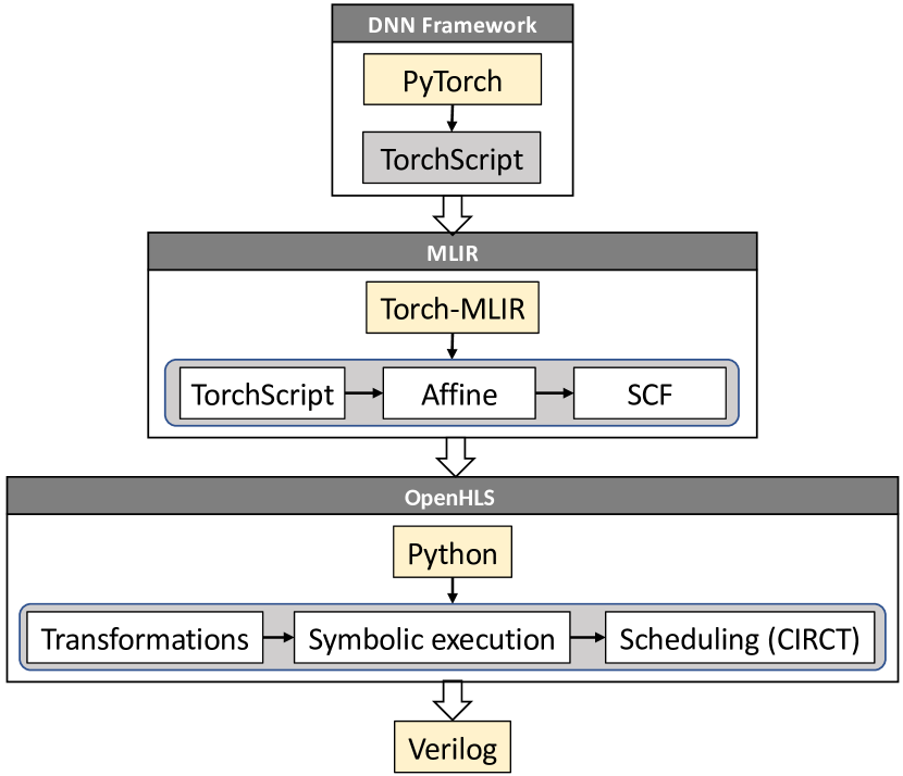
Figure 3. OpenHLS framework overview.

⬇

@conv2d(

) {

scf.for scf.for scf.for scf.for scf.for scf.for scf.for memref.store }

}

}

}

}

}

}

return }

Figure 4. scf dialect loop representation of Listing 1.

The benefits of translating scf dialect to Python are manifold: see Section 3.1. Ultimately, OpenHLS produces a representation of the DNN that is then fully scheduled by using the scheduling infrastructure in CIRCT (Oppermann et al., 2022) (an MLIR adjacent project). After scheduling, OpenHLS emits corresponding RTL (as Verilog).

OpenHLS delegates to the FloPoCo (de Dinechin, 2019) IP generator the task of generating pipelined implementations of the standard floating-point arithmetic operations (mulf, divf, addf, subf, sqrtf) at various precisions. In addition, we implement a few generic (parameterized by bit width) operators in order to support a broad range of DNN operations: two-operand maximum (max), unary negation (neg), and the rectified linear unit (relu). Transcendental functions, such as exp, are implemented by using a Taylor series expansion to $k$-th order (where $k$ is determined on a case-by-case basis). Note that FloPoCo’s floating-point representation differs slightly from IEEE754, foregoing subnormals and differently encoding zeroes, infinities and NaNs (for the benefit of reduced complexity) and our implementations max, neg, relu are adjusted appropriately.

We now discuss some aspects of OpenHLS in more detail.

3.1. Symbolic interpretation for fun and profit

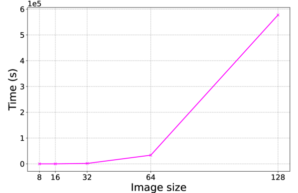
Figure 5. 3$\times$3-kernel convolution (cf. Listing 4) full unrolling time vs. input (square) image size, with store-load forwarding using MLIR’s -affine-scalrep pass. The longest time is 577,419 s ($\approx$160 h) for a loop nest with a trip count of 128$\times$128$\times$3$\times$3=147,456.

As noted in Section 2.2, maximizing concurrency and parallelism for a design entails unrolling loops and analyzing the data flow of their operations. As illustrated in Figure 5, the formally correct approach to unrolling loop nests can be prohibitively expensive in terms of runtime. In the case of BraggNN (see Listing 11), for example, the high cost of unrolling precluded effective search of the design space for a RTL representation achieving the target latency. Translating scf dialect to Python enables OpenHLS to overcome this barrier by enabling us to use the Python interpreter as a symbolic interpreter. Interpreting the resulting Python loop nests (i.e., running the Python program) while treating the arithmetic and memory operations on SSA values as operations on symbols (i.e., Python classes with overloaded methods) enables us to:

1. Partially evaluate functions of iteration variables (for example, %3 = arith.addi %i3, %i6) to determine array index operands of all stores and loads (for example, memref.load %input[%i1,%i5,%i3,%3,%4]) and thereupon perform memory dependence checks, thus transforming the problem of statically verifying memory dependence into one of checking assertions at runtime;

2. Unroll loops by recording each floating-point arithmetic operation executed while enforcing SSA; e.g., for a loop whose body has repeated assignments to the same SSA value (ostensibly violating SSA), we execute the loop and instantiate new, uniquely identified, symbols for the result of each operation;

3. Reconstruct all data flow through arithmetic operations and memory operations by interpreting memrefs as geometric symbol tables (i.e., symbol tables indexed by array indices rather than identifiers/names) and stores and loads as reads and writes on those symbol tables;

4. Swap evaluation rules in order to support various functional modes, e.g., evaluating floating-point arithmetic operations by using (Python) bindings to FloPoCo’s C++ functional models, thereby enabling behavioral verification of our designs.

See Table 6 for the translation rules from MLIR dialects to Python.

$\left\llbracket\texttt{MLIR}\right\rrbracket$	Python
|$\llbracket$|%5|$\rrbracket$|	v5 = Val("%5")
|$\llbracket$|memref<|$b\times c_{in}\times h\times w$|>|$\rrbracket$|	MemRef(|$b$|, |$c_{in}$|, |$h$|, |$w$|)
|$\llbracket$||$\perc$|5 = memref.load %input[%i1, %i5, %3, %4]|$\rrbracket$|	|$\llbracket$|%5|$\rrbracket$| = |$\llbracket$|%input|$\rrbracket$|.__getitem__((|$\llbracket$|%i1|$\rrbracket$|, |$\llbracket$|%i5|$\rrbracket$|, |$\llbracket$|%3|$\rrbracket$|, |$\llbracket$|%4|$\rrbracket$|))
|$\llbracket$| memref.store %9, %output[%i1, %i5, %3, %4]|$\rrbracket$|	|$\llbracket$|%output|$\rrbracket$|.__getitem__((|$\llbracket$|%i1|$\rrbracket$|, |$\llbracket$|%i5|$\rrbracket$|, |$\llbracket$|%3|$\rrbracket$|, |$\llbracket$|%4|$\rrbracket$|), |$\llbracket$|%9|$\rrbracket$|)
|$\llbracket$| scf.for %i1 = %c0 to |$b$| step %c1|$\rrbracket$|	for |$\llbracket$|%i1|$\rrbracket$| in range(|$\llbracket$|%c0|$\rrbracket$|, |$b$|, |$\llbracket$|%c1|$\rrbracket$|)
|$\llbracket$||$\perc$|3 = arith.addi %i3, %i6|$\rrbracket$|	|$\llbracket$|%3|$\rrbracket$| = |$\llbracket$|%i3|$\rrbracket$| + |$\llbracket$|%i6|$\rrbracket$|
|$\llbracket$||$\perc$|8 = arith.mulf %5, %6|$\rrbracket$|	|$\llbracket$|%8|$\rrbracket$| = |$\llbracket$|%5|$\rrbracket$|.__mul__(|$\llbracket$|%6|$\rrbracket$|)
|$\llbracket$||$\perc$|9 = arith.addf %7, %8|$\rrbracket$|	|$\llbracket$|%9|$\rrbracket$| = |$\llbracket$|%7|$\rrbracket$|.__add__(|$\llbracket$|%8|$\rrbracket$|)
|$\llbracket$||%|9 = arith.addf |%|7, |%|8|$\rrbracket$|!   \tabularnewline \noalign{\vskip1mm} \hline \noalign{\vskip1mm} \multicolumn{3}{c}{\mintinline{python}|$\llbracket$||%|9|$\rrbracket$| = fma(|$\llbracket$||%|5|$\rrbracket$|, |$\llbracket$||%|6|$\rrbracket$|, |$\llbracket$||%|7|$\rrbracket$|)!

Figure 6. Translation rules for mapping scf, arith, and memref dialects to Python.

3.2. AST transformations and verification

Prior to interpretation, OpenHLS performs some simple AST transformations on the Python generated from scf dialect:

1. Hoist globals: Move fixed DNN tensors (i.e., weights) out of the body of the generated Python function (OpenHLS translates the MLIR module corresponding to the DNN into a single Python function in order to simplify analysis and interpretation) and into the parameter list, for the purpose of ultimately exposing them at the RTL module interface.

2. Remove if expressions: DNN relu operations are lowered to the scf dialect as a decomposition into arith.cmpfugt and arith.select; this transformation recomposes them into a relu.

3. Remove MACs: Schedule sequences of load-multiply-add-store (common in DNN implementations) jointly, coalescing them into a single fmac operation.

4. Reduce fors: Implement the reduction tree structure for non-parallelizable loop nests mentioned in Section 3.3.

These transformations on the Python AST are simple (implemented with procedural pattern matching), extensible, and efficient (marginal runtime cost) because no effort is made to verify their formal correctness. Thus, OpenHLS trades formal correctness for development time performance. This tradeoff enables quick design space iteration, which for example, enabled us to achieve low latency implementations for BraggNN (see Section 4.2).

OpenHLS supports behavioral rather than formal verification. Specifically, OpenHLS can generate testbenches for all synthesized RTL. The test vectors for these testbenches are generated by evaluating the generated Python representation of the DNN on randomly generated inputs but with floating-point operations now evaluated using functional models of the corresponding FloPoCo operators. The testbenches can then be run using any IEEE 1364 compliant simulator. We run a battery of such testbenches (corresponding to various DNN operation types), using cocotb (Rosser, 2018) and iverilog (Williams, [n. d.]), as a part of our continuous integration (CI) process.

3.3. Scheduling

Recall that HLS must schedule operations during each clock cycle in a way that preserves the DNN’s data-flow graph. That schedule then informs the construction of a corresponding FSM. As already mentioned, scheduling an arbitrary DNN involves formulating and solving an ILP. In the resource-unconstrained case, due to the precedence relations induced by data flow, the constraint matrix of the associated ILP is a totally unimodular matrix and the feasible region of the problem is an integral polyhedron. In such cases, the scheduling problem can be solved optimally in polynomial time with a LP solver (Oppermann, 2019). In the resource-constrained case, resource constraints can also be transformed into precedence constraints by picking a particular (possibly heuristic) linear ordering on the resource-constrained operations. This transformation partitions resource-constrained operations into distinct clock cycles, thereby guaranteeing sufficient resources are available for all operations scheduled within the same clock cycle (Dai et al., 2018).

OpenHLS uses the explicit parallelism of the scf.parallel loop-nest representation to inform such a linear ordering on resource-constrained operations. By assumption, for loop nests which can be reprepresented as scf.parallel loop nests (see Listing 7), each instance of a floating-point arithmetic operation in the body corresponding to unique values of the iteration variables (e.g., %i1, %i2, %i3, %i4 for Listing 7) is independent of all other such instances, although data flow within a loop body must still be respected. This exactly determines total resource usage per loop nest; for example, the convolution in Listing 7 would bind to $2K_{i}$ DSPs (assuming mulf, addf bind to one DSP each), where:

$K_{i}\ \coloneqq$	$\left|\left\{\texttt{\%i1}=\texttt{\%c0}+\texttt{\%c1}\times\mathbb{N}\,\wedge\,\texttt{\%i1}<b\right\}\right|\ \times$
	$\left|\left\{\texttt{\%i2}=\texttt{\%c0}+\texttt{\%c1}\times\mathbb{N}\,\wedge\,\texttt{\%i2}<c_{out}\right\}\right|\ \times$
	$\left|\left\{\texttt{\%i3}=\texttt{\%c0}+\texttt{\%c1}\times\mathbb{N}\,\wedge\,\texttt{\%i3}<h\right\}\right|\ \times$
	$\left|\left\{\texttt{\%i4}=\texttt{\%c0}+\texttt{\%c1}\times\mathbb{N}\,\wedge\,\texttt{\%i4}<w\right\}\right|$

with $\texttt{\%c1}\times\mathbb{N}$ representing all multiples of %c1. That is to say, $K_{i}$ is the cardinality of the cartesian product of the iteration spaces of the parallel iteration variables.

⬇

@conv2d(

) {

scf.parallel (((|$b$|, |$c_{out}$|, |$h$|, |$w$|) step

(scf.for scf.for scf.for memref.store }

}

}

}

return }

Figure 7. Parallel loop representation of Listing 1, exhibiting explicitly the resource partitioning and ordering strategy we employ to construct a feasible schedule of operations.

Defining $K\coloneqq\max_{i}K_{i}$ across all scf.parallel loop nests, we can infer peak usage of any resource. Then, after indexing available hardware resources $j=1,\dots,K$, we can bind the operations of any particular loop nest. This leads to a linear ordering on resource-constrained operations such that operations bound to the same hardware resource index $j$ must be ordered according to their execution order during symbolic interpretation. Note that this ordering coincides with the higher-level structure of the DNN, which determines the ordering of scf.parallel loop nests (and thus interpretation order during execution of the Python program).

For DNN operations that lower to sequential loop nests rather than scf.parallel loop nests (e.g., sum, max, or prod), we fully unroll the loops and transform the resulting, sequential, operations into a reduction tree; we use As-Late-As-Possible scheduling (Baruch, 1996) amongst the subtrees of such reduction trees.

4. Evaluation

We evaluate OpenHLS both on individual DNN layers, and end-to-end, on our use-case BraggNN. We compare OpenHLS to Xilinx’s Vitis HLS by comparing the latencies and resource usages of the final designs generated by each. We also compare the runtimes of the tools themselves. Both OpenHLS and Vitis HLS produce Verilog RTL, on which we run a synthesis pass by using Xilinx’s Vivado. The particular FPGA target is Xilinx Alveo U280. We measure LUT, DSP, BRAM, and FF usage. For the DNN layer evaluations, we use FloPoCo (5,11)-floating point representations (5-bit exponent, 11-bit mantissa), corresponding to Vitis HLS’s IEEE half-precision IPs. We synthesize all designs for a 10 ns target clock period and report end-to-end latency as a product of the total schedule interval count of the design and achieved clock period (10-WNS, where WNS is the worst negative slack reported). In the case of Vitis HLS, which potentially explicitly pipelines the design and therefore implements with an initiation interval strictly less than the total schedule interval count, we report in terms of the best possible interval count (LatencyBest from the Vitis HLS reports). All other measurements are collected from Vivado synthesis reports. As Vitis HLS operates on C++ representations, we generate such a representation for our test cases by first lowering each DNN layer to the affine dialect and then applying the scalehls-translate tool of the ScaleHLS project (Ye et al., 2022) to emit C++. Importantly, we do not make any use of scalehls-opt optimization tool (of the same project).

Since our ultimate goal is low latency inference, and since the strategy that OpenHLS employs in the pursuit of this goal is loop unrolling, in order to produce a like for like comparison, we similarly unroll the representation that is passed to Vitis HLS. Thus, all Vitis HLS measurements are reported in terms of unroll factor: an unroll factor of $k$ corresponds to a $k$-fold increase in the number of statements in the body of a loop and commensurate $k$-fold decrease in the trip count of the loop. For loop nests, we unroll inside out: if $k$ is greater than the trip count $t$ of the innermost loop, we unroll the innermost loop completely and then unroll the enclosing loop by a factor of $k-t$. We do not perform any store-load forwarding during this preprocessing but we annotate all arrays with the directive array_partition complete dim=1 in order that Vitis HLS can effectively pipeline. All representations generated by OpenHLS correspond to full unrolling of the loop nests.

4.1. DNN layers

We evaluate OpenHLS vs. Xilinx’s Vitis HLS by comparing the latency of the final design on five DNN layer types, chosen to cover a range of arithmetic operations (mulf, divf, addf, subf, sqrtf) and data access patterns (iteration, accumulation, reduction):

• addmm(a, b, c): Matrix multiply: a $\times$ b + c;

• batch_norm_2d(num_features): Batch normalization over a 4D input (Ioffe and Szegedy, 2015);

• conv_2d(|$c_{in}$|, |$c_{out}$|, |$k$|): 2D convolution with bias, with $k\times k$ kernel, over a $b\times c_{in}\times h\times w$ input, producing $b\times c_{out}\times h^{\prime}\times w^{\prime}$ output;

• max_pool_2d(|$k$|, stride): 2D max pooling, with $k\times k$ kernel, and striding;

• soft_max: $\begin{aligned} \text{softmax}\left(\boldsymbol{x}\right)\coloneqq\left[\frac{\exp\left(x_{i}\right)}{\sum_{j}\exp\left(x_{j}\right)}\right]\end{aligned}$

The parameter values and input dimensions used during evaluation are summarized in Table 1.

Table 1. DNN layers used for evaluation of OpenHLS.

Layer	Parameter values	Input dimensions
addmm	N/A	$\texttt{a},\texttt{b},\texttt{c}:\left(16,16\right)$
batch_norm_2d	$\texttt{num\_features}=2$	$\texttt{input}:\left(10,2,3,3\right)$
conv_2d	$c_{in}=1,c_{out}=k=3$	$\texttt{input}:\left(1,1,16,16\right)$
max_pool_2d	$k=3,\texttt{stride}=2$	$\texttt{input}:\left(1,3,16,16\right)$
soft_max	N/A	$\texttt{input}:\left(1,3,16,16\right)$

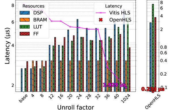
(a) addmm module

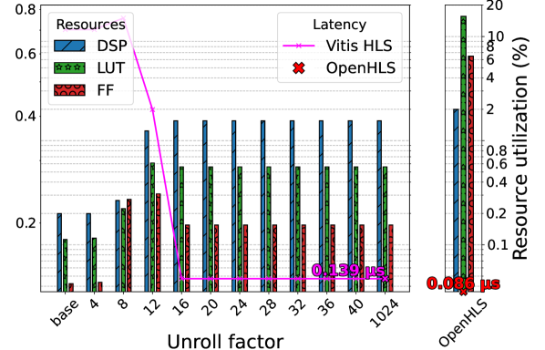
(b) batch_norm_2d module

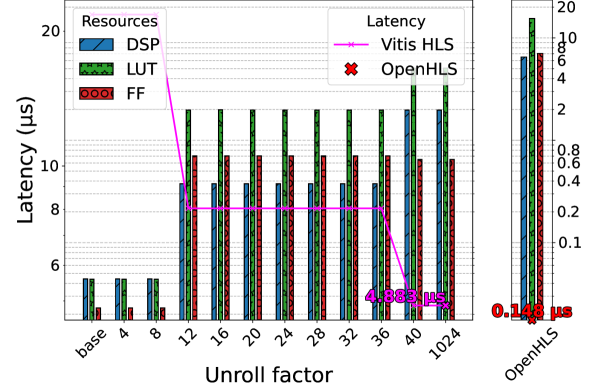
(c) conv_2d module

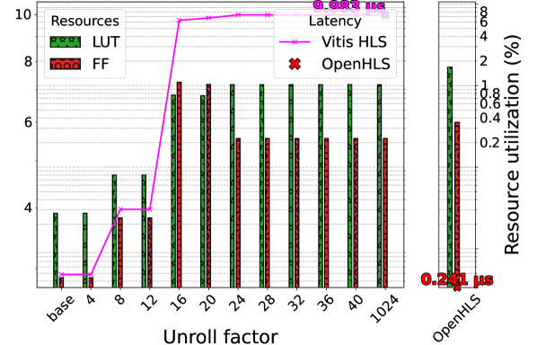
(d) max_pool_2d module

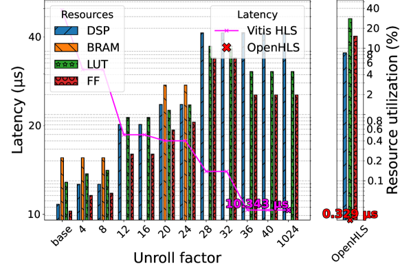
(e) soft_max module

Figure 8. Vitis HLS vs. OpenHLS resource usage and latency vs. unroll factor for five DNN modules, exhibiting the large runtime cost incurred in using Vitis HLS to search the design space (of possible low-latency designs for each layer). The lines give latencies (left axes); the bars give the % of the resource used (right axes). All y-scales are log.

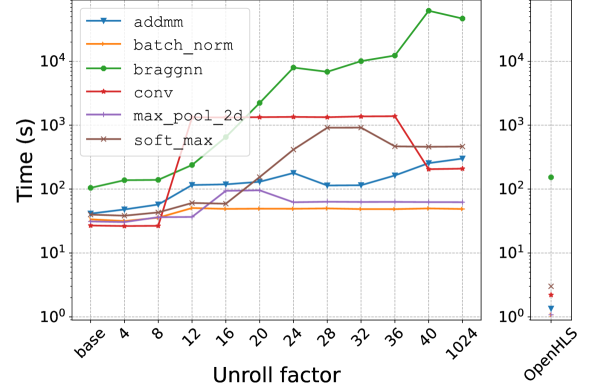
Figure 9. Vitis HLS vs. OpenHLS runtime vs. unroll factor, illustrating the large runtime cost incurred in using Vitis HLS to search over possible low-latency BraggNN designs.

Figure 8 shows Vitis HLS vs. OpenHLS resource usage and latency vs. unroll factor and Figure 9 shows the runtimes of Vitis HLS as function of increasing unroll factor. We observe that while Vitis HLS end-to-end latencies decrease with increased unroll factor, they never match that achieved by OpenHLS. Even at an unroll factor of 1024 (which corresponds to fully unrolled for all loop nests comprising these layer types), Vitis HLS is only within 10$\times$ of OpenHLS. We attribute this to Vitis HLS’s inability to pipeline effectively, due to its inability to eliminate memory dependencies, either through store-load forwarding or further array partitioning. Conversely, OpenHLS’s ability to effectively perform store-load forwarding is evident in the complete lack of BRAM usage: all weights are kept on FFs or LUTs. While infeasible for larger designs (which would be constrained by the number of available FFs), this unconstrained usage of FFs is acceptable for our use case. The increasing latency (as a function of unroll factor) in the max_pool_2d case is due to Vitis HLS’s failure to meet timing, i.e., while the interval count decreases as a function of unroll factor, the clock period increases.

4.2. BraggNN case study

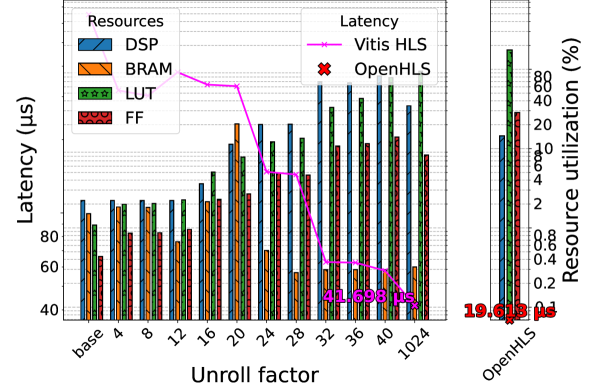
Figure 10. BraggNN Vitis HLS vs. OpenHLS resource usage and latency vs. unroll factor (with both at half-precision) throughout the design space of possible low-latency designs.

High-energy diffraction microscopy enables non-destructive characterization for a broad class of single-crystal and polycrystalline materials. A critical step in a typical HEDM experiment is an analysis to determine precise Bragg diffraction peak characteristics. Peak characteristics are typically computed by fitting the peaks to a probability distribution, e.g., Gaussian, Lorentzian, Voigt, or Pseudo-Voigt. As noted in Section 1, HEDM experiments can collect data at more than 80 GB/s. These data rates, though more modest than at the LHC, merit exploring low latency approaches in order to enable experiment modalities that depend on measurement-based feedback (i.e., experiment steering).

⬇

BraggNN(|$s$|)(

(cnn_layers_1): Conv2d(|$s \times16 $|, kernel=3, stride=1)

(nlb): NLB(

(theta_layer): Conv2d(|$s \times16 $|, |$s \times8 $|, kernel=1, stride=1)

(phi_layer): Conv2d(|$s \times16 $|, |$s \times8 $|, kernel=1, stride=1)

(g_layer): Conv2d(|$s \times16 $|, |$s \times8 $|, kernel=1, stride=1)

(out_cnn): Conv2d(|$s \times8 $|, |$s \times16 $|, kernel=1, stride=1)

(soft): Softmax()

)

(cnn_layers_2): Sequential(

(0): ReLU()

(1): Conv2d(|$s \times16 $|, |$s \times8 $|, kernel=3, stride=1)

(2): ReLU()

(3): Conv2d(|$s \times8 $|, |$s \times2 $|, kernel=3, stride=1)

(4): ReLU()

)

(dense_layers): Sequential(

(0): Linear(in_features=|$s \times50$|, out_features=|$s \times16 $|)

(1): ReLU()

(2): Linear(in_features=|$s \times16 $|, out_features=|$s \times8 $|)

(3): ReLU()

(4): Linear(in_features=|$s \times8 $|, out_features=|$s \times4 $|)

(5): ReLU()

(6): Linear(in_features=|$s \times4 $|, out_features=2)

(7): ReLU()

)

)

Figure 11. BraggNN model architecture for scaling factors s=1,2.

BraggNN (Liu et al., 2022b), a DNN aimed at efficiently characterizing Bragg diffraction peaks, achieves a throughput (via batch inference) of approximately 22 µs/sample on a state-of-the-art GPU: a large speedup over classical pseudo-Voigt peak fitting methods, but still far short of the 1 µs/sample needed to handle 1 MHz sampling rates. In addition, the data-center class GPU such as a NVIDIA V100 (or even a workstation class GPU such as a NVIDIA RTX 2080Ti) required to run the current BraggNN implementation cannot be deployed at the edge, i.e., adjacent or proximal to the high energy microscopy equipment. With the goal of reducing both per-sample time and deployment footprint, we applied OpenHLS to the PyTorch representation of BraggNN(s=1) (see Listing 11) and achieved a RTL implementation which synthesizes to a 1238 interval count design that places, routes, and meets timing closure for a clock period of 10 ns (for a Xilinx Alveo U280). The design consists of a three stage pipeline with the longest stage measuring 480 intervals, for a throughput of 4.8 µs/sample. See Figure 10 for a comparison with designs generated by Vitis HLS (using the same flow as in 4).

The most challenging aspect of implementing BraggNN was minimizing latency while satisfying compute resource constraints (LUTs, DSPs, BRAMs) and achieving routing closure, i.e., not exceeding available routing resources and avoiding congestion. We made two design choices to reduce resource consumption. The first was to reduce the precision used for the floating-point operations, from half precision to FloPoCo (5,4)-precision (5-bit exponent, 4-bit mantissa), a choice justified by examination of the distribution of the weights of the fully trained BraggNN (see Figure 12).

Reducing the precision enabled the second design choice, to eliminate BRAMs from the design, since, at the lower precision, all weights can be represented as registered constants. The reduced precision also drove the Vivado synthesizer to infer implementations of the floating-point operations that make no use of DSPs, likely becaue the DSP48 hardware block includes a 18-bit by 25-bit signed multiplier and a 48-bit adder (gui, 2021), neither of which neatly divides the bit width of FloPoCo (5,4)-precision cores. (The actual width for FloPoCo (5,4)-precision is 12 bits: 1 extra bit is needed for the sign and 2 for handling of exceptional conditions.)

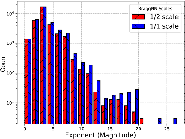
Figure 12. OpenHLS weights exponent distribution, illustrating the narrow distribution of observed weight exponents thereby justifying reduced precision.

Achieving routing closure was difficult due to the nature of the Xilinx’s UltraScale architecture, of which the Alveo U280 is an instance. The UltraScale architecture achieves its scale through Stacked Silicon Interconnect (SSI) technology (Leibson et al., 2013), which implies multiple distinct FPGA dies, called Super Logic Regions (SLRs), on the same chip, connected by interposers. Adjacent SLRs communicate with each other over a limited set of Super Long Lines (SLLs), which determine the maximum bus width that spans two SLRs. On the Alveo U280 there are exactly 23,040 SLLs available between adjacent SLRs and at (5,4)-precision BraggNN(s=1) needs 23,328 SLLs between SLR2 and SLR1. [We route from SLR2 to SLR1 the outputs of cnn_layers_1 (1$\times$16$\times$9$\times$9$\times$12 wires) and soft(theta_layer$\times$ phi_layer)$\times$g_layer (1$\times$8$\times$9$\times$9$\times$12 wires).] Thus, we further reduced the precision to (5,3). Finally, since multiple dies constitute independent clock domains, the SLLs that cross SLRS are sensitive to hold time violations due to the higher multi-die variability (rap, [n. d.]). This multi-die variability leads to high congestion if not addressed. Thus, routing across SLRs needs to be handled manually, using placement and routing constraints for logic in each SLR and the addition of so-called “launch” and “latch” registers in each SLR. Figure 13 illustrates the effect of using launch and latch registers as well as placement and routing constraints.

(a) BraggNN fails to achieve routing closure without placement and routing constraints and launch and latch registers.

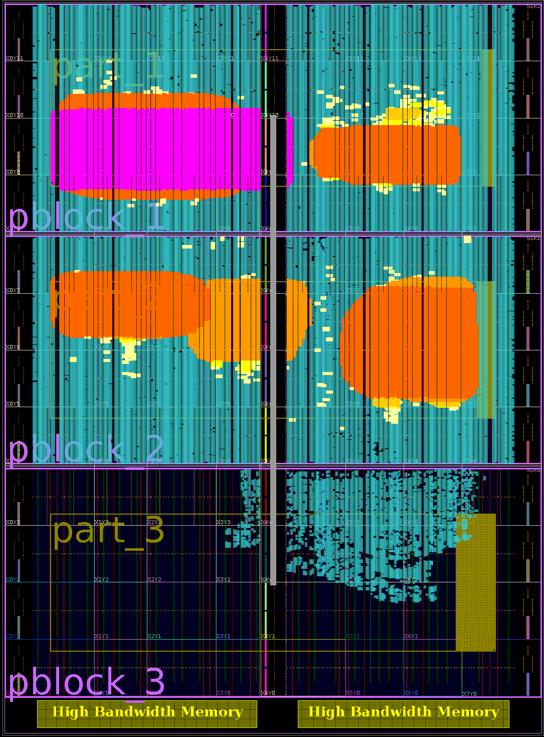
(b) BraggNN achieves routing closure with use of per SLR placement and routing constraints (pblock_1, pblock_2, pblock_3) and launch and latch registers (not highlighted).

Figure 13. Congestion maps for BraggNN on a Xilinx Alveo U280. Magenta indicates areas of high congestion.

Thus, these design choices (in combination with compiler level optimizations performed by OpenHLS) plus careful management of routing constraints enable us to lower, compile, synthesize, place, and route BraggNN(s=1) to Xilinx’s Alveo U280 at a throughput of 4.8 µs/sample: ~5$\times$ higher latency than the target 1 µs/sample, but a ~4$\times$ improvement over the PyTorch GPU implementation.

5. Conclusion

We have presented OpenHLS, an MLIR-based HLS compilation framework that supports translating DNN models to RTL without the use of commercial HLS tools. The OpenHLS end-to-end compilation pipeline provides a PyTorch front-end and Verilog emission back-end. An extensible Python intermediate layer supports use-case-specific optimizations (e.g., store-load forwarding) that are not possible otherwise. Experimental results demonstrate that OpenHLS outperforms, in terms of end-to-end latency, Vitis HLS on a range of DNN layer types and on a case-study DNN.

We note three directions for future work, primarily with respect to scheduling: (1) Better integration between the Python layer and MLIR: it is preferable that the transformations on the Python representation could make use of various MLIR facilities, such as affine analysis, for the purposes of exploring loop transformations that improve latency; (2) Expanding the set of scheduling algorithms available: for example, resource aware scheduling (Dai et al., 2018); and (3) Integration of scheduling-aware placement and vice-versa (placement-aware scheduling): currently OpenHLS can be used to inform placement but does not explicitly emit placement constraints (see Section 4.2); a more precise approach, such as in (Guo et al., 2021), would potentially enable better pipelining and thus higher throughput.

References

- (1)
- rap ([n. d.]) Create placed and routed DCP to cross SLR. https://www.rapidwright.io/docs/SLR_Crosser_DCP_Creator_Tutorial.html. Accessed: 2022-10-15.
- gui (2021) 2021. UltraScale Architecture DSP Slice. Technical Report. XiLinx. https://docs.xilinx.com/v/u/en-US/ug579-ultrascale-dsp
- Aaij et al. (2020) Roel Aaij et al. 2020. Allen: A high-level trigger on GPUs for LHCb. Computing and Software for Big Science 4, 1 (2020), 1–11.
- Abadi et al. (2016) Martín Abadi et al. TensorFlow: Large-Scale Machine Learning on Heterogeneous Distributed Systems. https://doi.org/10.48550/ARXIV.1603.04467
- Alzubaidi et al. (2021) Laith Alzubaidi et al. 2021. Review of deep learning: Concepts, CNN architectures, challenges, applications, future directions. Journal of Big Data 8, 1 (2021), 1–74.
- Ashari et al. (2015) Arash Ashari et al. 2015. On Optimizing Machine Learning Workloads via Kernel Fusion. 50, 8 (2015), 173–182. https://doi.org/10.1145/2858788.2688521
- Baruch (1996) Zoltan Baruch. 1996. Scheduling algorithms for high-level synthesis. ACAM Scientific Journal 5, 1-2 (1996), 48–57.
- Bohm Agostini et al. (2022) Nicolas Bohm Agostini et al. 2022. Bridging Python to Silicon: The SODA Toolchain. IEEE Micro (2022). https://doi.org/10.1109/MM.2022.3178580
- Bondhugula (2020) Uday Bondhugula. Polyhedral compilation opportunities in MLIR. https://acohen.gitlabpages.inria.fr/impact/impact2020/slides/IMPACT_2020_keynote.pdf.
- Canis et al. (2013) Andrew Canis et al. 2013. LegUp: An Open-Source High-Level Synthesis Tool for FPGA-Based Processor/Accelerator Systems. ACM Trans. Embed. Comput. Syst. 13, 2, Article 24 (2013). https://doi.org/10.1145/2514740
- Chen et al. (2015) Tianqi Chen et al. MXNet: A Flexible and Efficient Machine Learning Library for Heterogeneous Distributed Systems. https://doi.org/10.48550/ARXIV.1512.01274
- Chen et al. (2018) Tianqi Chen et al. 2018. TVM: An automated end-to-end optimizing compiler for deep learning. In 13th USENIX Symp. Operating Systems Design & Impl. 578–594.
- Chen et al. (2016) Tianqi Chen, Bing Xu, Chiyuan Zhang, and Carlos Guestrin. Training Deep Nets with Sublinear Memory Cost. https://doi.org/10.48550/ARXIV.1604.06174
- Collaboration (2020) LHCb Collaboration. 2020. Comparison of particle selection algorithms for the LHCb Upgrade. Technical Report. https://cds.cern.ch/record/2746789
- Dai et al. (2018) Steve Dai, Gai Liu, and Zhiru Zhang. 2018. A Scalable Approach to Exact Resource-Constrained Scheduling Based on a Joint SDC and SAT Formulation. In ACM/SIGDA Intl Symposium on Field-Programmable Gate Arrays. 137–146.
- de Dinechin (2019) Florent de Dinechin. 2019. Reflections on 10 Years of FloPoCo. In IEEE 26th Symposium on Computer Arithmetic. 187–189.
- Duarte et al. (2018) J. Duarte et al. 2018. Fast inference of deep neural networks in FPGAs for particle physics. Journal of Instrumentation 13, 07 (2018), P07027–P07027.
- Ferrandi et al. (2021) Fabrizio Ferrandi et al. 2021. Bambu: an Open-Source Research Framework for the High-Level Synthesis of Complex Applications. In 58th ACM/IEEE Design Automation Conference. IEEE, 1327–1330.
- Gligorov (2015) Vladimir Gligorov. 2015. Real-time data analysis at the LHC: present and future. In NIPS Workshop on High-energy Physics and Machine Learning, Vol. 42. 1–18.
- Gligorov and Williams (2013) V V Gligorov and M Williams. 2013. Efficient, reliable and fast high-level triggering using a bonsai boosted decision tree. J. Instrumentation 8, 02 (2013).
- Grainge et al. (2017) Keith Grainge et al. 2017. Square Kilometre Array: The radio telescope of the XXI century. Astronomy reports 61, 4 (2017), 288–296.
- Guo et al. (2021) Licheng Guo et al. 2021. AutoBridge: Coupling Coarse-Grained Floorplanning and Pipelining for High-Frequency HLS Design on Multi-Die FPGAs. In ACM/SIGDA International Symposium on Field-Programmable Gate Arrays. 81–92.
- Hammer et al. (2021) M. Hammer, K. Yoshii, and A. Miceli. 2021. Strategies for on-chip digital data compression for X-ray pixel detectors. Journal of Instrumentation 16, 01 (2021), P01025–P01025. https://doi.org/10.1088/1748-0221/16/01/p01025
- Hattori et al. (2022) Momoko Hattori, Naoki Kobayashi, and Ryosuke Sato. Gradual Tensor Shape Checking. https://doi.org/10.48550/ARXIV.2203.08402
- Ioffe and Szegedy (2015) Sergey Ioffe and Christian Szegedy. Batch Normalization: Accelerating Deep Network Training by Reducing Internal Covariate Shift. https://doi.org/10.48550/ARXIV.1502.03167
- Lattner et al. (2020) Chris Lattner et al. MLIR: A compiler infrastructure for the end of Moore’s Law. https://doi.org/10.48550/ARXIV.2002.11054
- Leibson et al. (2013) Steve Leibson et al. 2013. Xilinx ultrascale: The next-generation architecture for your next-generation architecture. Xilinx White Paper WP435 143 (2013).
- Liu et al. (2018) Yizhi Liu et al. 2018. Optimizing CNN Model Inference on CPUs. (2018). https://doi.org/10.48550/ARXIV.1809.02697
- Liu et al. (2022a) Yongtao Liu et al. 2022a. Exploring physics of ferroelectric domain walls in real time: Deep learning enabled scanning probe microscopy. Advanced Science (2022).
- Liu et al. (2019) Zhengchun Liu et al. 2019. Deep learning accelerated light source experiments. In IEEE/ACM 3rd Workshop on Deep Learning on Supercomputers. IEEE, 20–28.
- Liu et al. (2022b) Zhengchun Liu et al. 2022b. BraggNN: fast X-ray Bragg peak analysis using deep learning. IUCrJ 9, 1 (2022), 104–113.
- Maleki et al. (2011) Saeed Maleki et al. 2011. An evaluation of vectorizing compilers. In International Conference on Parallel Architectures and Compilation Techniques. IEEE, 372–382.
- McMullin et al. (2022) J McMullin et al. 2022. The Square Kilometre Array project update. In Ground-based and Airborne Telescopes IX, Vol. 12182. SPIE, 263–271.
- Nane et al. (2016) Razvan Nane et al. 2016. A Survey and Evaluation of FPGA High-Level Synthesis Tools. IEEE Transactions on Computer-Aided Design of Integrated Circuits and Systems 35, 10 (2016), 1591–1604. https://doi.org/10.1109/TCAD.2015.2513673
- Oppermann (2019) Julian Oppermann. 2019. Advances in ILP-based Modulo Scheduling for High-Level Synthesis. Ph. D. Dissertation. Technische Universität, Darmstadt. http://tuprints.ulb.tu-darmstadt.de/9272/
- Oppermann et al. (2022) Julian Oppermann et al. 2022. How to make hardware with maths: An introduction to CIRCT’s scheduling infrastructure. In European LLVM Developers’ Meeting.
- Paszke et al. (2017) Adam Paszke et al. 2017. Automatic differentiation in PyTorch. In 31st Conference on Neural Information Processing Systems.
- Patton et al. (2018) Robert M Patton et al. 2018. 167-Pflops deep learning for electron microscopy: From learning physics to atomic manipulation. In SC’18. IEEE, 638–648.
- Rajopadhye (2002) Sanjay V Rajopadhye. 2002. Dependence Analysis and Parallelizing Transformations. In The Compiler Design Handbook.
- Rausch et al. (2022) Oliver Rausch et al. 2022. DaCeML: A Data-Centric Optimization Framework for Machine Learning. In 36th ACM International Conference on Supercomputing.
- Rosser (2018) Benjamin John Rosser. Cocotb: a Python-based digital logic verification framework. https://docs.cocotb.org.
- Rotem et al. (2018) Nadav Rotem et al. Glow: Graph Lowering Compiler Techniques for Neural Networks. https://doi.org/10.48550/ARXIV.1805.00907
- Sharma et al. (2016) Hardik Sharma et al. 2016. From high-level deep neural models to FPGAs. In 49th Annual IEEE/ACM International Symposium on Microarchitecture. 1–12.
- Silva and Elangovan (2021) Sean Silva and Anush Elangovan. Torch-MLIR. https://mlir.llvm.org/OpenMeetings/2021-10-07-The-Torch-MLIR-project.pdf.
- Takamaeda-Yamazaki (2015) Shinya Takamaeda-Yamazaki. 2015. Pyverilog: A Python-based hardware design processing toolkit for Verilog HDL. In International Symposium on Applied Reconfigurable Computing. Springer, 451–460.
- Williams ([n. d.]) Stephen Williams. Icarus Verilog, 1998–2020. http://iverilog.icarus.com.
- Ye et al. (2022) Hanchen Ye et al. 2022. ScaleHLS: A New Scalable High-Level Synthesis Framework on Multi-Level Intermediate Representation. In IEEE International Symposium on High-Performance Computer Architecture.
- Zhang et al. (2008) Zhiru Zhang et al. 2008. AutoPilot: A Platform-Based ESL Synthesis System. In High-Level Synthesis. Springer Netherlands, Dordrecht, 99–112.
- Zheng et al. (2022) S. Zheng et al. 2022. NeoFlow: A Flexible Framework for Enabling Efficient Compilation for High Performance DNN Training. IEEE Transactions on Parallel and Distributed Systems 33, 11 (2022), 3220–3232.