Workload-Balanced Pruning for
Sparse Spiking Neural Networks

Abstract

Pruning for Spiking Neural Networks (SNNs) has emerged as a fundamental methodology for deploying deep SNNs on resource-constrained edge devices. Though the existing pruning methods can provide extremely high weight sparsity for deep SNNs, the high weight sparsity brings a workload imbalance problem. Specifically, the workload imbalance happens when a different number of non-zero weights are assigned to hardware units running in parallel, which results in low hardware utilization and thus imposes longer latency and higher energy costs. In preliminary experiments, we show that sparse SNNs ($\sim$98% weight sparsity) can suffer as low as $\sim$59% utilization. To alleviate the workload imbalance problem, we propose u-Ticket, where we monitor and adjust the weight connections of the SNN during Lottery Ticket Hypothesis (LTH) based pruning, thus guaranteeing the final ticket gets optimal utilization when deployed onto the hardware. Experiments indicate that our u-Ticket can guarantee up to 100% hardware utilization, thus reducing up to 76.9% latency and 63.8% energy cost compared to the non-utilization-aware LTH method.

I Introduction

Spiking Neural Networks (SNNs) have gained tremendous attention towards ultra-low-power machine learning [1]. SNNs leverage spatio-temporal information of unary spike data to achieve energy-efficient processing in resource-constrained edge devices [2, 3]. However, in the case of large-scale tasks such as image classification, the model size of SNNs significantly increases. Unfortunately, edge devices typically have limited on-chip memory, rendering large-scale SNN deployment unpractical. To this end, recent works have proposed various unstructured SNN pruning techniques to achieve high weight sparsity in SNNs [4, 5].

Although unstructured pruning manages to compress the SNN models into the available memory resources, sparse SNNs encounter a workload-imbalance problem [6]. The workload-imbalance problem comes from the conventional weight stationary dataflow [7] adopted in sparse accelerators [8, 9, 10]. In weight stationary dataflow, filters are divided into several groups and kept stationary inside processing elements (PEs) for filter reuse. However, different filter groups inevitably have different densities of non-zero weights, due to the random weight connections from the unstructured pruning. As a result, different PEs end up with unbalanced workloads. Since all PEs run in parallel, PEs with fewer workloads need to wait for the PE that has the largest workload. This results in low utilization and imposes idle cycles, which increases the running latency and leakage of energy waste.

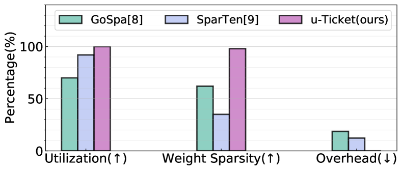
Figure 1: Comparison between u-Ticket and state-of-the-art workload balance methods. Overall, u-Ticket recovers the PE utilization up to $100\%$ for extremely sparse networks with 98% weight sparsity (here, we consider VGG-16). Please note that u-Ticket does not introduce any hardware area overhead, and thus is the best fit for SNNs (↑: the higher is the better, ↓: the lower is the better).

To address the workload-imbalance problem, various methods have been proposed in the prior sparse accelerator designs. However, they cannot be efficiently applied to SNNs for the following reasons. (1) Requiring extra hardware: The prior methods require extra hardware (e.g., deep FIFOs or permuting units) [9, 8, 11, 12, 13] to balance the workloads. For instance, applying the hardware-based (FIFOs [8] and permuting networks [9]) workload balancing methods to SNNs require approximately 18% and 13% of extra chip area (see Fig. 1). Consequentially, the improvements in PE utilization are at the cost of additional hardware resources, which should be avoided for SNNs whose running environments are typically resource-constrained edge devices. (2) Limited to low sparsity: As shown in Fig. 1, the solutions from prior sparse accelerators [8, 9] only work on low sparsity (roughly 60% and 35% on VGG-16) which is not sufficient for SNNs’ extremely low-power edge deployment. Moreover, the workload-imbalance problem naturally gets more difficult to solve at high weight sparsity regime. Hence, the exploration of workload balancing for extremely sparse networks ($>95\%$ weight sparsity) is missing in prior works. Considering the above-mentioned problems, we need an SNN-friendly solution to address the workload imbalance.

To this end, we propose u-Ticket, an iterative workload-balanced pruning method for SNNs that can effectively achieve high weight sparsity and minimize the workload imbalance problem simultaneously. Our method is based on Lottery Ticket Hypothesis (LTH) [14] which states that sub-networks with similar accuracy can be found in over-parameterized networks by repeating training-pruning-initialization stages. Different from the standard LTH method [4] where the pruned networks are naively used for the next round, we either remove or recover weight connections to balance workloads across all PEs before sending the networks to re-initialization (see Fig. 2).

Compared to prior workload-balancing methods (see Fig. 1), the u-Ticket approach improves PE utilization by up to 100% (70% for [8] and 92% for [9]) while maintaining filter sparsity of 98% (60% for [8] and 35% for [9]), at iso-accuracy with the standard LTH-based pruning baseline [4]. Furthermore, since our method balances the workload during the pruning process, u-Ticket does not incur any additional hardware overhead for deployment.

We summarize the key contributions as follows:

1. We propose u-Ticket which discovers highly sparse SNNs with optimal PE utilization. The discovered sparse SNN model achieves a similar level of accuracy, weight sparsity, and spike sparsity with the standard LTH baseline [4] while improving the utilization up to $100\%$.

2. By balancing the workload, u-Ticket reduces the running latency and energy cost by up to $76.9\%$ and $63.8\%$, respectively, compared to the standard LTH method.

3. We extend the prior sparse accelerator[8] and propose an energy estimation model for sparse SNNs.

4. To validate the proposed u-Ticket, we conduct experiments on two representative deep architectures (i.e., VGG-16 [15] and ResNet-19 [16]) across three public datasets including CIFAR10 [17], Fashion-MNIST [18] and SVHN [19].

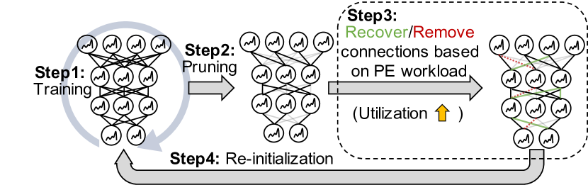
Figure 2: Illustration of the concept of the proposed u-Ticket. Our u-Ticket consists of training (step1), pruning (step2), adjusting weight connections based on workload (step3), and re-initialization (step4). We repeat these steps for multiple rounds. Note, the standard LTH method consists of training (step1), pruning (step2), and re-initialization (step4), which does not consider the utilization of the pruned SNNs.

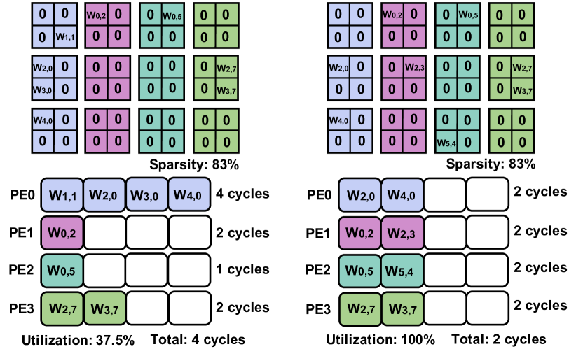
Figure 3: Example utilization and latency resulted from imbalance and balanced workload under the same model sparsity. With the unstructured pruning, non-zero weights will have a random distribution across four groups, thus leading to unbalanced workloads across PEs as shown on the left side (PE0 has four weights assigned, while PE1 and PE2 only have one).

II Background

II-A Spiking Neural Networks

Spiking Neural Networks (SNNs) process the unary temporal signal through multi-layer weight connections. Instead of ReLU neuron for a non-linear activation, recent SNN works use a Leaky-Integrate-and-Fire (LIF) neuron which contains a memory called membrane potential. The membrane potential captures the temporal spike information by storing incoming spikes and generating output spikes accordingly. Suppose a LIF neuron $i$ has a membrane potential $u_{i}^{t}$ at timestep $t$. We can formulate the discrete neuronal dynamics [20, 21] by:

$$u_{i}^{t}=\lambda u_{i}^{t-1}+\sum_{j}w_{ij}s^{t}_{j}.$$ (1)

Here, $\lambda$ is the leaky factor for decaying the membrane potential through time. The $s^{t}_{j}$ stands for the output spike from a neuron $j$ at timestep $t$. The $w_{ij}$ denotes a weight connection between neuron $j$ in the previous layer and neuron $i$ in the current layer. If the membrane potential reaches a firing threshold, the neuron generates an output spike, and the membrane potential is reset to zero. Similar to ANNs, we train the weight connection $w_{ij}$ in all layers. Our weight optimization is based on the recently proposed surrogate gradient learning, which assumes approximated gradient function for the non-differentiable LIF neuron [22]. We use $tanh(\cdot)$ approximation following the previous work [21].

II-B Lottery Ticket Hypothesis

Lottery Ticket Hypothesis (LTH) [14] has been proposed where they found a dense neural network contains sparse sub-networks (i.e., winning tickets) with similar accuracy compared to the original dense network. The winning tickets are founded by multiple rounds of magnitude pruning operations. Specifically, suppose we have a dense network $f(x;\theta)$ with randomly-initialized parameter weights $\theta\in\mathbb{R}^{n}$. In the first round, the dense network $f(x;\theta)$ is trained to convergence (step1 in Fig. 2). Based on the trained weights, we prune $p\%$ weight connections with the lowest absolute weight values (step2 in Fig. 2). We represent this pruning operation as a binary mask $m\in\{0,1\}^{n}$. In the next round, we reinitialize the pruned network with the original initialization parameters $f(x;\theta\odot m)$ (step4 in Fig. 2), where $\odot$ represents the element-wise product. The training-pruning-initialization stages are repeated for multiple rounds. In the SNN domain, Kim et al.[4] recently applied LTH to deep SNNs, resulting in high weight sparsity ($\sim$98%) for VGG and ResNet architectures. However, they do not consider the workload imbalance problem in sparse SNNs. Different from the previous work, we adjust weight connections for improving utilization at each pruning round step3, which reduces up to $77\%$ latency and $64\%$ energy cost compared to the standard LTH [4] while maintaining both sparsity and accuracy.

II-C Workload Imbalance Problem

In the context of neural network accelerators, dataflow refers to the input and weight mapping strategy on the hardware. To this effect, recent works [10, 9, 8, 23, 24] have demonstrated the efficacy of the weight stationary dataflow towards efficient deployment of sparse networks and SNNs. For weight-stationary dataflow, different weights are cast to different PEs and stay inside the PE until they are maximally reused across all the relevant computations. More specifically, during the running time, depending on the memory capacity of the hardware, each layer’s filter kernels will be grouped in a chosen pattern and sent to each PE. As shown in Fig. 3, due to the randomness in unstructured pruning, the number of non-zero elements (or workload) allocated to each PE varies significantly. Moreover, the workload imbalance is persistent irrespective of the grouping method chosen. Note, here we define the number of non-zero weights assigned to a PE as the workload.

In this case, the wasted resources in PEs are based on the difference between the largest workload and the average of all other workloads. To quantitatively measure the portion of non-wasted resources, we use the utilization metric[6], given by

$$\mu=1-\frac{T_{max}-T_{avg}}{T_{max}}\cdot\frac{n}{n-1},$$ (2)

$T_{max}$ and $T_{avg}$ are the slowest and the average processing time among the PEs. $n$ is the number of PEs. The metric quantifies the percentage of processing time that the rest of the PEs, excluding the slowest one, is engaging in useful work.

In Fig. 4, we show how the utilization degrades as the weight sparsity of the SNN increases in the standard LTH method [4]. The preliminary result shows that in the final round, the utilization can be as low as $59\%$ on VGG-16 CIFAR10. Here, we assume that the total number of PEs is 16 and the utilization is averaged across all layers (weighted by parameter count).

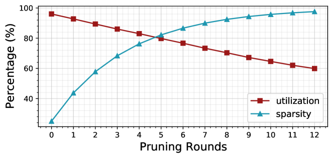
Figure 4: Sparsity and utilization across pruning rounds for the standard LTH method without utilization awareness. The pruning is done for 13 rounds on VGG-16 being trained for image classification on CIFAR10 with 16 PEs.

III u-Ticket

To resolve the workload imbalance problem, we propose u-Ticket where we achieve high utilization in sparse SNNs during iterative pruning. In this section, we first present the algorithm to train sparse SNNs while maintaining high utilization. We then provide details of the proposed PE design and the energy model to map the u-Ticket on the hardware.

III-A Algorithmic Approach

Algorithm 1 u-Ticket

Input: SNNs $f(x;\theta)$ with randomly-initialized parameter weights $\theta\in\mathbb{R}^{n}$, connectivity mask $m_{i}\in\{0,1\}^{n}$ at iteration $i$, total pruning round $N_{Round}$, total number of layer $L$, number of PEs $n$, Workload of a PE $d$, Workload list of a layer $W^{l}$.
Output: Pruned $f(x;\theta_{trained}\odot m_{N})$

1:initialize $m_{1}$ with $1$ $\triangleright$ No pruning in the first round

2:for $i\leftarrow$ 1 to $N_{Round}$ do

3:    $f(x;\theta\odot m_{i})$ $\triangleright$ Iterative magnitude pruning

4:    $f(x;\theta_{trained}\odot m_{i})\leftarrow Train(f(x;\theta\odot m_{i}))$

5:    $\hat{m}_{i}\leftarrow Prune(f(x;\theta_{trained}\odot m_{i})$)

6:    for $l\leftarrow$ 1 to $L$ do $\triangleright$ Layer-wise adjustment

7:         $W^{l}\leftarrow GetWorkloadList(f(x;\theta^{l}_{trained}\odot\hat{m}^{l}_{i}),n$)

8:         $d^{l}_{avg}\leftarrow GetAverage(W^{l})$

9:         for $d$ in $W_{l}$ do$\triangleright$ Adjust each workload group

10:             if $d<d^{l}_{avg}$ then

11:                 $m^{l}_{i+1}\leftarrow RandomlyRecover(\hat{m}^{l}_{i},d_{avg}-d)$

12:             else

13:                 $m^{l}_{i+1}\leftarrow RandomlyRemove(\hat{m}^{l}_{i},d-d_{avg})$

14:             end if

15:         end for

16:    end for

17:end for

Our u-Ticket pruning consists of multiple rounds similar to LTH [14]. For each round, we train the networks till convergence, prune the low-magnitude weight connections, balance the workload of PEs by recovering or removing the weight connections, and finally re-initialize the weights. The main idea is to ensure a balanced workload between PEs after unstructured pruning in each round.

The overall u-Ticket process is described in Algorithm 1. For each round, the pruned SNN from the previous round is re-initialized. After that, the model is trained and pruned where we obtain connectivity mask $\hat{m}_{i}$ with imbalanced PE workloads. To increase the utilization, we first compute the workload for each PE, constructing the PE workload list $W^{l}$ for each layer. Based on the $W^{l}$, we calculate the average workload $w_{avg}^{l}$ for layer $l$. Then, we go through each workload $w$ in $W^{l}$, and randomly recover ($w_{avg}-w$) number of weight connections if the PE’s workload $w$ is smaller than the average workload $w_{avg}^{l}$. Otherwise, the number of weight connections is pruned by ($w-w_{avg}$). After the workload adjustment, every workload $w$ will have the same magnitude, to ensure the optimal utilization $\mu$. We repeat the above-mentioned stages for $N$ rounds.

In our method, we use average workload $w_{avg}^{l}$ across all PEs at layer $l$ as the reference to recover/remove weight connections. The reason behind such design choice is as follows: (1) If we look at only partial PE workloads to decide on a reference workload, it will bring a sub-optimal solution. (2) The cost of checking all PE workloads is negligible compared to the overall iterative training-pruning-initialization process. We find that on an RTX 2080Ti GPU, the time cost of our workload-balancing method is only 0.11% of one complete LTH searching round.

III-B Hardware Mapping

III-B1 Processing Elements (PEs)

To get an accurate energy estimation, we need to map the sparse SNN to a proper hardware design. We develop our PE design based on [8], one of the state-of-the-art sparse accelerators, to support the running of sparse SNNs. Please note that our method of balancing the workloads works on any sparse accelerator design as long as it utilizes the weight stationary dataflow.

First, the non-zero weights, input spikes, and their corresponding metadata (index) are read from the DRAM. The weights are represented in weight sparsity pattern (WSP) [8], while the spike activations are represented in standard compressed sparse row (CSR) format. We use four timesteps for the SNN in our experiments, thus we can group every two activations into one byte (each activation has four unary spikes.)

Then, an activation processing unit (APU, outside PEs) filters out the zero activation (0-spikes across four timesteps) and sends the non-zero activation together with their position indices (decoded from CSR) to the PE arrays. The position indices help to match the non-zero weights and activation in 2-D convolution.

At the PE level, each PE contains four 16-bit AND gates, 256 24-bit accumulators, and one 1024 $\times$ 16 bits SRAM-based scratch-pad. We further extend the 256 accumulators with 256 LIF units for generating the output spikes. Each LIF unit is equipped with four 24-bit registers for storing the membrane potential across four timesteps.

Fig. 5 illustrates the overall architecture and the computation flow inside the PE. We process the network in a tick-batched manner [23]. At step , the non-zero weights together with their WSPs are mapped to each PE. At step , the spike activation $S_{in}$ together with their position indices are sent to PE. Based on the weight’s WSP and the activation’s position index, the selector unit will output the matched non-zero weight. At step and , the dot-product operations between the input spike and the matched weights are carried out, and the partial sums are stored according to their position index. At step , the partial sums for each time step are sequentially sent to the LIF units to generate the output spikes for each time step. Note that steps - need to be repeated four times for matching the four timesteps used in our SNN model (only 1 bit of $S_{in}$ is cast to the PE at a time in step ).

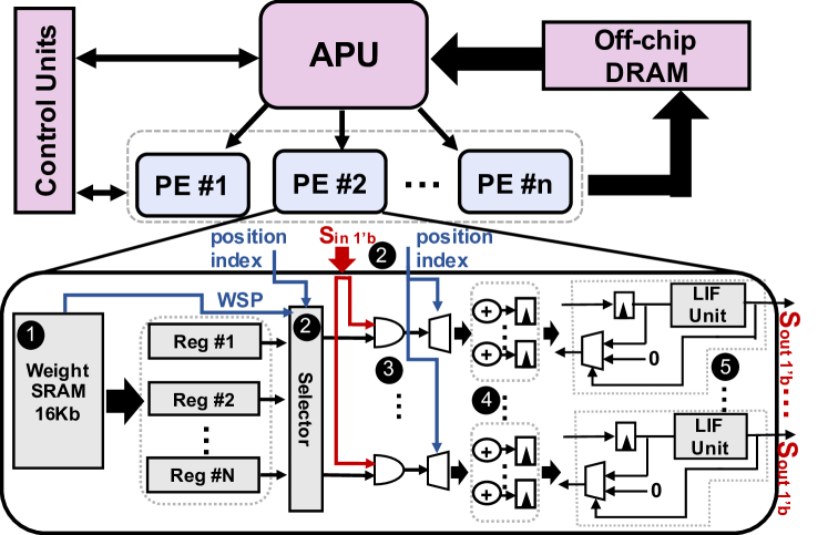
Figure 5: Overall architecture and the detailed inner architecture of PE. Here APU denotes the activation processing unit.

III-B2 Energy Modeling

We do the simulation for the full architecture. Since u-Ticket balances the workloads between PEs, the majority of the improvements can be found at the PE level. Thus, we focus on energy estimation at the PE level in this work. We extend the energy model from [24] to estimate the total energy:

$$E_{total}=N_{work}\cdot(E_{PE}^{d}\cdot(1-S_{in}^{spa})+E_{PE}^{l})+N_{idle}\cdot E_{PE}^{l},$$ (3)

where $E_{PE}^{d}$ and $E_{PE}^{l}$ are the dynamic and leakage energy of a single PE processing one input spike. As shown in [24], there is no extra cost for skipping the zero-spike computation in SNNs. Thus, we directly apply the term of spike sparsity, $S_{in}^{spa}$, in Eqn. 3 to consider the dynamic energy saving by skipping the zero spikes. Here $N_{work}$ is defined as the total work cycles in which PEs are doing useful work and $N_{idle}$ denotes the total cycles in which PEs are waiting in an idle state.

IV EXPERIMENT

IV-A Experimental Settings

IV-A1 Software Configuration

First, to validate the u-Ticket pruning method, we evaluate our u-Ticket methods on three public datasets: CIFAR10 [17], Fashion-MNIST [18], and SVHN [19]. We choose two representative deep network architectures: VGG-16 [15] and ResNet-19 [16]. We implement the networks on PyTorch and set the timesteps $T$ to 4 for all experiments. We use state-of the-art direct encoding technique that has been shown to train SNNs on image classification datasets with very few timesteps. We use the same training configurations used in [4].

IV-A2 Hardware Configuration

We report the utilization, latency, work cycles, and idle cycles based on our PyTorch-based simulator which simulates the running-time distribution of the weights to PEs. We use the weights grouping method as in [8, 24] with 16 PEs. The PE level energy is estimated with the model in Section III-B2 with all computing units synthesized in Synopsys Design Compiler at 400MHz using 32nm CMOS technology and the memory units simulated in CACTI. We set the standard LTH method [4] without utilization-awareness as our baseline and use the same estimation model to get the speed-up and energy results.

TABLE I: Comparison of accuracy, sparsity of filters and spikes between our method and the standard LTH method.

Dataset Method Acc.(%) Sparsity(%) Sparsity(%) (filters) (spikes) VGG-16[15] CIFAR10 LTH[4] 91.0 98.2 84.8 u-Ticket (ours) 90.7 98.4 85.9 FMNIST LTH[4] 94.6 98.2 83.9 u-Ticket (ours) 94.0 98.5 81.4 SVHN LTH[4] 95.5 98.2 84.9 u-Ticket (ours) 94.8 98.5 80.1 ResNet-19[16] CIFAR10 LTH[4] 91.0 97.6 64.1 u-Ticket (ours) 90.3 98.4 68.3 FMNIST LTH[4] 94.4 98.2 60.1 u-Ticket (ours) 93.3 99.0 62.9 SVHN LTH[4] 95.1 97.6 63.6 u-Ticket (ours) 94.6 98.6 68.2

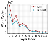
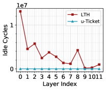
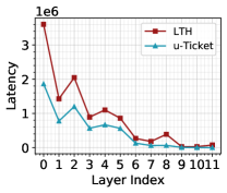
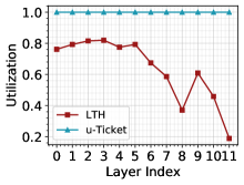
(a)	(b)	(c)	(d)

Figure 6: The layerwise performance comparison between LTH and u-Ticket on four metrics, i.e., (a) work cycles, (b) idle cycles, (c) latency, (d) utilization. We conduct experiments with VGG-16 architecture on CIFAR10.

IV-B Experimental Results

IV-B1 Validation Result

We summarize the validation results in Table I. The results confirm that our method works well for deep SNNs (less than $\sim$1% accuracy drop). We also compare the sparsity of filters and spikes between these two methods. u-Ticket has a slightly higher filter sparsity, due to the extra reduction in weight connections to ensure balanced workloads for each PE. At the same time, u-Ticket keeps a similar level of spike sparsity on VGG-16 and has better spike sparsity on ResNet-19. While higher spike sparsity will bring better energy efficiency, a spike sparsity that is too high will cause an accuracy drop in deep SNNs [25]. This explains the accuracy-sparsity tradeoff on ResNet-19 (on average 0.76% accuracy drop with 3.5% sparsity gain).

IV-B2 Hardware Performance

We consider four metrics in this section (i.e., work cycles, idle cycles, latency, and utilization).

• Work cycles ($N_{work}$ in Eqn. 4): Sum of total work cycles for every PE across all the layers in the network.

• Idle cycles ($N_{idle}$ in Eqn. 4): Sum of total idle cycles for every PE across all the layers in the network.

• Latency: Time required by PEs to process all the layers in the network. The latency is normalized with respect to the time required for a PE to process one input spike.

• Utilization: We use Eqn. 2 to compute the utilization for each layer. To compute the utilization of the network, we calculate the weighted average utilization.

The hardware improvement results are summarized in Table II. By iteratively applying the utilization recovery during the pruning, u-Ticket can recover the utilization up to $100\%$ in the final pruning round, thus reducing almost all the idle cycles for PEs. Because of the re-balance of workloads among PEs, the network can leverage more parallelism from the PE array, thus significantly reducing the running latency. The number of work cycles stays similar on both networks. We further visualize the layerwise speedup results for VGG-16 on CIFAR10 in Fig. 6. Overall, the layerwise work cycles and latency share similar trends between the two methods. Furthermore, u-Ticket has a larger number of idle cycle reductions on earlier layers due to the larger feature map sizes.

TABLE II: Comparison of work cycles, idle cycles, latency, and utilization between u-Ticket and the standard LTH.

Dataset Method Work Idle Latency Utilization ($\times 1e8$) ($\times 1e8$) ($\times 1e8$) VGG-16[15] CIFAR10 LTH[4] 1.34 0.41 0.11 0.59 u-Ticket (ours) 0.94 0.00 0.06 1.00 FMNIST LTH[4] 1.10 0.42 0.10 0.57 u-Ticket (ours) 0.81 0.00 0.05 1.00 SVHN LTH[4] 1.15 0.69 0.12 0.47 u-Ticket (ours) 0.86 0.00 0.05 1.00 ResNet-19[16] CIFAR10 LTH[4] 1.66 1.73 0.21 0.31 u-Ticket (ours) 1.10 0.00 0.07 1.00 FMNIST LTH[4] 1.26 1.89 0.20 0.27 u-Ticket (ours) 0.73 0.00 0.05 1.00 SVHN LTH[4] 1.27 1.34 0.16 0.30 u-Ticket (ours) 0.84 0.00 0.05 1.00

IV-B3 Energy Performance

In this section, we further show the energy efficiency improvements of u-Ticket over the standard LTH baseline. The energy differences are visualized in Fig. 7 (a), from which we observe that the energy benefits of balancing the workloads are huge. For CIFAR10, FMNIST, and SVHN, we manage to reduce the energy cost by $41.8\%$, $35.4\%$, and $37.2\%$ on VGG-16, and $55.5\%$, $63.8\%$, and $56.1\%$ on ResNet-19.

The main source of energy cost reduction comes from the elimination of idle cycles and the reduction of latency, which ultimately reduces the leakage energy of the hardware. ResNet-19, whose network is deeper, suffers more from the workload imbalance problem and thus has more idle cycles and longer latency compared to VGG-16. By eliminating almost all the idle cycles, u-Ticket brings more energy cost reduction to ResNet-19 compared to VGG-16.

IV-B4 Analysis of Sparsity

We study the effects of the u-Ticket method under different weight sparsity. We measure the energy difference between u-Ticket and the LTH baseline at different pruning rounds for both ResNet-19 and VGG-16 on the CIFAR10 dataset. The result is visualized in Fig. 7 (b). As observed, with an increase in weight sparsity, the benefits of using u-Ticket get larger. This is due to the degradation of the utilization in LTH as aforementioned in Fig. 4.

IV-B5 Analysis of #PEs

We further study the effects of changing the number of PEs. We run the u-Ticket for VGG-16 on CIFAR10 with 2, 4, 8, 16, 32, and 64 PEs, and illustrate the results in Table. III. While the energy cost only slightly changes with the increasing number of PEs, the latency decreases linearly. Considering that the area of PE arrays will also linearly increase with the number of PEs, we conduct most of our experiments with 16 PEs, which is a suitable trade-off point.

TABLE III: Changes in normalized energy cost and normalized latency as the total number of PEs increases. Results are normalized with respect to the energy and latency of 2 PEs.

Number of PEs 2 4 8 16 32 64 Normalized Energy 1 1.01 1.02 0.95 1.02 1.04 Normalized Latency 1 0.49 0.25 0.12 0.06 0.03

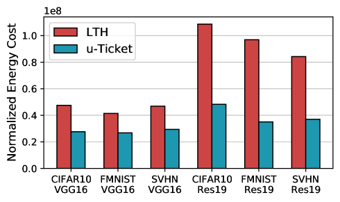
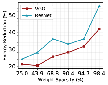
(a)	(b)

Figure 7: (a) Comparison of the normalized energy cost between two networks and across three datasets. The energy results are normalized to the energy required by a PE to process one input spike. (b) Percentage of normalized energy reduction compared to the LTH baseline for different weight sparsity.

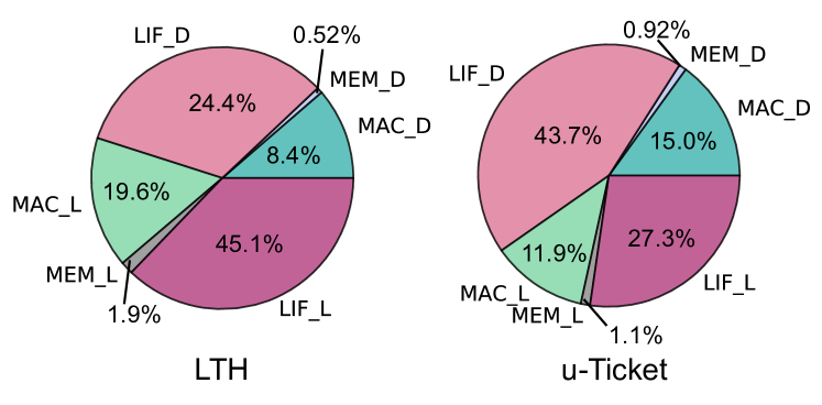
Figure 8: Comparison of the energy breakdown between u-Ticket and the LTH baseline. MAC_L, MEM_L, and LIF_L denote the leakage energy for MAC, LIF, and memory operation, while MAC_D, MEM_D, and LIF_D denote their dynamic energy.

IV-B6 Energy Breakdown

In Fig. 8, we show the energy breakdown comparison between u-Ticket and the LTH baseline on ResNet-19 for the CIFAR10 dataset. The energy components are the dynamic and leakage energy of MAC operation, LIF operation, and MEM operation (reading of SRAM-based scratchpad). We observe that the leakage energy for both MAC and LIF operation is significantly reduced in u-Ticket due to the elimination of the idle cycles. Expectedly, the portion of the dynamic energy of MAC and LIF operation increases.

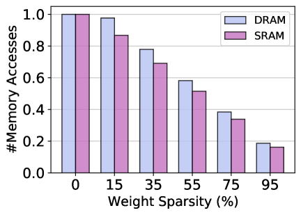
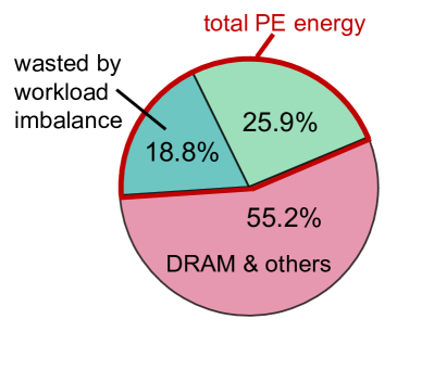
(a)	(b)

Figure 9: (a) Normalized DRAM and SRAM accesses comparison across different weight sparsity. (b) The component breakup of the total energy for LTH baseline with 95% sparsity. Both results are shown for VGG-16 with CIFAR10.

IV-B7 System Level Study

Finally, we study the behavior of the overall system of sparse SNNs. In Fig. 9 (a), we show how the total DRAM and SRAM access (normalized with respect to dense SNN) decrease with increasing weight sparsity. Furthermore, we find that in the extremely high weight sparsity regime, the PE level energy starts to take a significant portion of the total energy ($\sim$ 45% on VGG-16 with CIFAR10). As a result, after applying u-Ticket to balance the PE workloads, we manage to reduce approximately $19\%$ of the total energy at the system level as shown in Fig. 9 (b).

V Conclusion

In this work, we propose u-Ticket, a utilization-aware LTH-based pruning method that solves the workload imbalance problem in SNNs. Unlike prior works, u-Ticket recovers the utilization during pruning, thus avoiding additional hardware to balance the workloads during deployment. Additionally, at iso-accuracy, u-Ticket improves PE utilization by up to 100% compared to the standard LTH-based pruning method while maintaining filter sparsity of 98%. Moreover, u-Ticket reduces the running latency by up to 77% and energy cost by up to 64% compared to standard LTH baseline.

References

- [1] K. Roy et al., “Towards spike-based machine intelligence with neuromorphic computing,” Nature, vol. 575, no. 7784, pp. 607–617, 2019.
- [2] M. Davies et al., “Loihi: A neuromorphic manycore processor with on-chip learning,” IEEE Micro, vol. 38, no. 1, pp. 82–99, 2018.
- [3] F. Akopyan et al., “Truenorth: Design and tool flow of a 65 mw 1 million neuron programmable neurosynaptic chip,” IEEE TCAD, vol. 34, no. 10, pp. 1537–1557, 2015.
- [4] Y. Kim, Y. Li, H. Park, Y. Venkatesha, R. Yin, and P. Panda, “Exploring lottery ticket hypothesis in spiking neural networks,” in European Conference on Computer Vision. Springer, 2022, pp. 102–120.
- [5] L. Deng et al., “Comprehensive snn compression using admm optimization and activity regularization,” IEEE TNNLS, 2021.
- [6] L. DeRose et al., “Detecting application load imbalance on high end massively parallel systems,” in EuroPar, 2007.
- [7] Y.-H. Chen et al., “Eyeriss: A spatial architecture for energy-efficient dataflow for convolutional neural networks,” ISCA, 2016.
- [8] C. Deng et al., “Gospa: an energy-efficient high-performance globally optimized sparse convolutional neural network accelerator,” in ISCA, 2021.
- [9] A. Gondimalla et al., “Sparten: A sparse tensor accelerator for convolutional neural networks,” in MIRCRO, 2019.
- [10] A. Parashar et al., “Scnn: An accelerator for compressed-sparse convolutional neural networks,” ISCA, 2017.
- [11] S. Han et al., “Eie: Efficient inference engine on compressed deep neural network,” ISCA, 2016.
- [12] H. Kung et al., “Packing sparse convolutional neural networks for efficient systolic array implementations: Column combining under joint optimization,” in ASPLOS, 2019.
- [13] S. Han et al., “Ese: Efficient speech recognition engine with sparse lstm on fpga,” in FPGA, 2017.
- [14] J. Frankle et al., “The lottery ticket hypothesis: Finding sparse, trainable neural networks,” arXiv:1803.03635, 2018.
- [15] K. Simonyan et al., “Very deep convolutional networks for large-scale image recognition,” arXiv:1409.1556, 2014.
- [16] K. He et al., “Deep residual learning for image recognition,” in CVPR, 2016.
- [17] A. Krizhevsky et al., “Learning multiple layers of features from tiny images,” 2009.
- [18] H. Xiao et al., “Fashion-mnist: a novel image dataset for benchmarking machine learning algorithms,” arXiv:1708.07747, 2017.
- [19] Y. Netzer et al., “Reading digits in natural images with unsupervised feature learning,” 2011.
- [20] Y. Wu et al., “Spatio-temporal backpropagation for training high-performance spiking neural networks,” Frontiers in neuroscience, vol. 12, p. 331, 2018.
- [21] W. Fang et al., “Incorporating learnable membrane time constant to enhance learning of spiking neural networks,” in ICCV, 2021.
- [22] E. O. Neftci et al., “Surrogate gradient learning in spiking neural networks,” IEEE Signal Processing Magazine, vol. 36, pp. 61–63, 2019.
- [23] S. Narayanan et al., “Spinalflow: An architecture and dataflow tailored for spiking neural networks,” in ISCA, 2020.
- [24] R. Yin et al., “Sata: Sparsity-aware training accelerator for spiking neural networks,” arXiv:2204.05422, 2022.
- [25] Y. Li et al., “Differentiable spike: Rethinking gradient-descent for training spiking neural networks,” NeurIPS, 2021.