Accelerating Evolution Through Gene Masking
and Distributed Search

Abstract.

In building practical applications of evolutionary computation (EC), two optimizations are essential. First, the parameters of the search method need to be tuned to the domain in order to balance exploration and exploitation effectively. Second, the search method needs to be distributed to take advantage of parallel computing resources. This paper presents BLADE (BLAnket Distributed Evolution) as an approach to achieving both goals simultaneously. BLADE uses blankets (i.e., masks on the genetic representation) to tune the evolutionary operators during the search, and implements the search through hub-and-spoke distribution. In the paper, (1) the blanket method is formalized for the (1 + 1)EA case as a Markov chain process. Its effectiveness is then demonstrated by analyzing dominant and subdominant eigenvalues of stochastic matrices, suggesting a generalizable theory; (2) the fitness-level theory is used to analyze the distribution method; and (3) these insights are verified experimentally on three benchmark problems, showing that both blankets and distribution lead to accelerated evolution. Moreover, a surprising synergy emerges between them: When combined with distribution, the blanket approach achieves more than $n$-fold speedup with $n$ clients in some cases. The work thus highlights the importance and potential of optimizing evolutionary computation in practical applications.

1. Introduction

Automatic configuration, often called AutoML or meta-learning, has recently emerged as an important topic in machine learning (Elsken et al., 2019; Liang et al., 2019, 2021). Complex machine learning systems depend on several hyperparameters that are difficult to set right by hand, and therefore machine learning itself is harnessed to optimize them.

Likewise, the efficacy of an evolutionary computation approach often relies on the appropriate calibration of its operators. This paper proposes a new method for doing so automatically as part of the evolutionary search itself. The idea is to use a mask, i.e. a blanket, on the genotype to focus the search on specific parts of the problem. The masks are constructed dynamically throughout the search, and help focus it on parts that are the most important. In a sense, they play a role similar to attention heads in transformer neural networks (Vaswani et al., 2017), but adapted to population-based search.

A related practical challenge in machine learning is parallelization. As machine learning systems grow in size, there is a growing need for distributing the computation across multiple computing resources, including multiple cores on a single machine, multiple nodes in a cluster, and multiple resources in the cloud. While evolutionary computation generally parallelizes well, the method of distribution of evaluations and evolutionary operations has a large effect. The hub-and-spoke method is often preferable for maximum scalability and flexibility.

Putting blankets and distribution together, this paper proposes BLADE as an effective new method for accelerated evolution. Each of its components is first formalized and characterized theoretically, leading to predictions of possible speedups. These predictions are then confirmed in practical experiments with the $(1+1)EA$ optimization method on three optimization benchmarks, i.e.  AllOnes, OneMax, and LeadingOnes. The results reveal a surprising synergy between blankets and distribution that allows more than $n$-fold speedups with $n$ clients. In future work, the BLADE approach may be extended to other algorithms and applications, and can thus serve as a foundation for accelerated evolution in practice.

2. Background

This section reviews prior work related to BLADE both in automatic parameter tuning and in distributed evolutionary computation.

2.1. Parameter Optimization

All problem-solving methods rely on a number of parameters that have to be set appropriately for the method to function properly. In genetic algorithms, they include settings for the population size, the mutation rate and extent, the type of crossover, the selection method, the size of the elite set, the number of offspring, etc. They can be set up by hand through a laborious trial and error process, or a learning method such as evolution itself can be used to discover good settings.

For instance, in bilevel evolution, low-level evolution searches for solutions while high-level evolution searches for the best parameters for low-level evolution (Sinha et al., 2014; Liang and Miikkulainen, 2015). Bilevel evolution is expensive because it often requires running many low-level optimizations to evaluate the fitness of high-level individuals. Furthermore, there is a growing body of evidence suggesting that operator settings and other aspects of the configurations should be adapted dynamically in response to changes in the fitness of the population (Stützle et al., 2022; Ansótegui et al., 2009; Tuson and Ross, 1998; Hassanat et al., 2019; Papa and Doerr, 2020; Doerr et al., 2019; Buskulic and Doerr, 2019).

The blanket method establishes such a dynamic optimization mechanism: The settings of the search operator are adjusted as part of the search itself over the course of the run.

2.2. Distributed Evolution

There are several different methods for distributing an evolutionary process across multiple clients, and each method has its own advantages and disadvantages.

Synchronous distribution (Sudholt, 2015; Yang et al., 2019; Raghul and Jeyakumar, 2021; Hassani and Treijs, 2009): The evolution engine partitions the population, assigns each partition to an external worker to evaluate, and waits for all the evaluations to return before forming the population for the next generation. This method is simple, but it only scales well when the worker clients are machines with similar speed and connectivity; otherwise, time is wasted waiting for the slowest clients to finish their work. This approach can also be slow for large populations because there is a high communication overhead for distributing individuals.

Asynchronous population evaluation (Sudholt, 2015; Yang et al., 2019; Raghul and Jeyakumar, 2021; Hassani and Treijs, 2009) starts like the synchronous method, but the engine only waits until a part of the population has been evaluated before generating the next population. This method improves efficiency but may lose diversity.

Island model (Whitley et al., 1998): While the above methods rely on the star topology of distribution, the island model applies to a variety of topologies such as a ring or hypercube. The evolution engines themselves are distributed, and they migrate good solution candidates between themselves using peer-to-peer connections. This method is asynchronous and can generate a lot of diversity at scale. On the other hand, decentralization of evolution engines makes harvesting the best candidates difficult, and the peer-to-peer connections may become an overhead, especially when using highly connected topologies on different physical machines. Therefore, the island model is most suitable for parallel evolution on a single machine with many cores rather than distributing it over a network of machines.

Hub and spoke model (O’Reilly et al., 2013): This model also uses the star topology, but the clients (spokes) are full evolution engines. They evaluate candidates asynchronously on different partitions of the data and the results are aggregated in a centralized server (hub). The main advantage of this method is that it can be easily distributed over a very large network of diverse computing resources. Also, each client has only one external connection to the hub, and therefore it is possible to add or remove clients in an asynchronous manner. On the other hand, the hub may become overwhelmed with a very large number of clients. In such a situation, a method of load-balancing can be implemented.

In sum, the choice of distribution method depends on the specific requirements of the evolutionary algorithm and the computational resources available. For many evolutionary computation implementations, the hub-and-spoke model offers the best advantages, and will thus be used for BLADE as well.

3. Method

This section presents the details of the BLADE method. Intuition and theoretical formulation are first given for blankets and distribution separately, and these methods are then brought together to full BLADE. The discussion focuses on the optimization of binary strings with $(1+1)EA$. Possibilities for extending BLADE to other representations and search methods will be discussed in Section 5.

3.1. Blanket-based Search

The blanket method refers to the process of masking parts of a candidate solution so that they cannot be modified by the evolutionary operators such as mutation for $(1+1)EA$. It is a way to focus the search on those solution elements that make progress most likely.

3.1.1. Method Description

The blanket method involves modifying the mutation rate of bits in a binary string of length $N$ according to another binary string, i.e. the blanket, which can be any one of the $2^{N}$ such strings except all zeros and all ones. The mutation rate $\mu$ is modified by the factor of $\frac{N}{N-{\mathrm{len(blanket)}}}$.

For example, if $N=5$, $\mu=1/4$, and the blanket is ”$01011$”, then $\mathrm{len(blanket)}=3$, and the second, fourth, and fifth bits are preserved, and the first and third bits are mutated independently with the modified mutation probability $\mu_{\mathrm{b}}=\frac{1}{4}*\frac{5}{5-3}=\frac{5}{8}$. If $\mu_{\mathrm{b}}$ exceeds 1.0, it is clipped to 1.0, meaning that all bits not under the blanket are flipped deterministically. Algorithm 1 shows a modified version of $(1+1)EA$ that incorporates the blanket method.

Algorithm 1 Blankets only (non-distributed BLADE)

  Initialization:

  Sample $x\in\{0,1\}^{N}$ uniformly at random and evaluate $f(x)$

  Optimization:

  for $t=1,2,3,...$ do

        Offspring generation with blanket:

        Calculate mutation rate $\mu$

        Sample blanketLength from $[1,N-1]$ randomly

        Set blanket $\leftarrow$ flip blanketLength random bits in $\{0\}^{N}$

        Set $\mu_{\mathrm{b}}\leftarrow\min(1,\mu(\frac{N}{N-\emph{blanketLength}}))$

        Sample $y\in\{0,1\}^{N}$ at random with $p(1)=\mu_{\mathrm{b}}$

        Set $\emph{blanket}\leftarrow\emph{blanket}\land y$ ($\land$ is bitwise AND)

        Create $x^{*}\leftarrow x\oplus$ blanket ($\oplus$ is bitwise XOR)

        Selection:

        if $f(x^{*})\geq f(x)$ then

                 $x\leftarrow x^{*}$

        end if

  end for

3.1.2. Theoretical Formulation

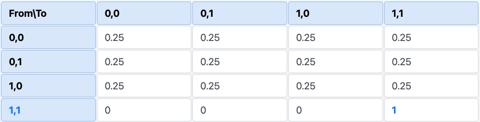
(a) Example transition matrix without blankets

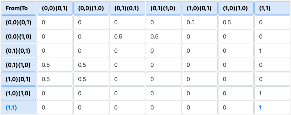
(b) Example transition matrix with blankets

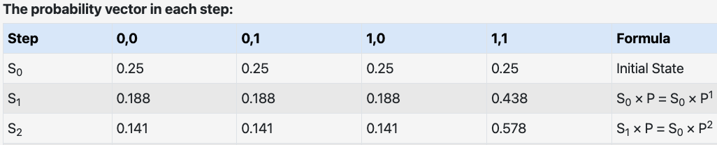
$\dots$

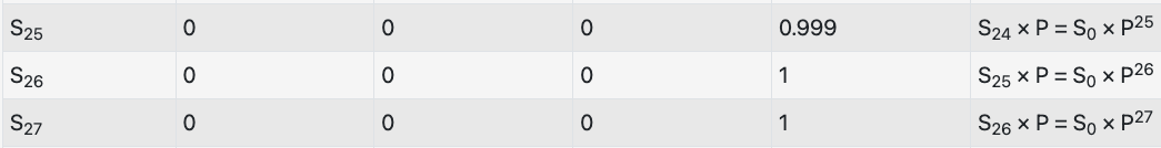
(c) Convergence without blankets

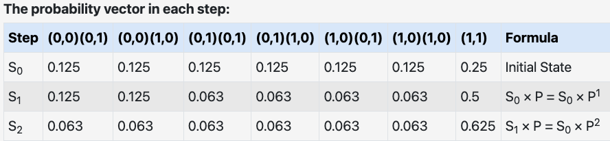
$\dots$

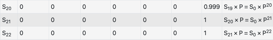
(d) Convergence with blankets

Figure 1. A comparison of convergence with and without blankets on a 2-bit AllOnes problem is shown using transition matrices (a) and (b). The presence of two possible blankets for each state in (a) results in twice as many states in (a), except for the last converging state of (1,1). The subdominant eigenvalue is 0.75 for matrix (a) and 0.71 for matrix (b), indicating faster theoretical convergence with blankets. The convergence process is depicted in (c) and (d), starting from a randomly chosen initial state $S_{0}$ with uniform probability. The process takes 26 transitions to converge without blankets, and only 21 transitions with blankets, confirming the theoretical advantage of using blankets in the search.

The blanket method may initially seem counterintuitive: It may help search if it masks those parts of the string that are indeed part of the solution, but it may also hinder search if it masks parts where further mutations are needed. Without further knowledge of the problem domain or a method for dynamically constructing blankets, its potential benefits and drawbacks may cancel out. A simple formalization is helpful in showing why this is not a problem, and blankets can indeed speed up the search process.

Consider $(1+1)EA$ on a 2-bit version of the AllOnes problem: Starting from random bits, each bit gets independently mutated at each iteration with the probability of $\frac{1}{2}$ until both bits are one. This process can be formalized as a Markov chain, i.e. a random process in which the future state of the system depends only on its current state and not its past history (Gagniuc, 2017). A transition matrix stores the probabilities of the system moving from one state to another, with zero indicating that a transition is not possible. An absorbing state is a state that cannot be left once it has been entered; it is represented by a row with a single non-zero element of 1.

Since there are $2^{2}=4$ different combinations of two bits, the transition matrix is of size $4\times 4$. A possible such matrix is shown in Figure 1(a). The rows represent the current states, the columns the possible next states, and each cell the probability of the corresponding transition. Once the system gets to the state in the bottom row it stays there forever; otherwise, it can transition from any state to any other state with a probability of 0.25.

With two bits, there are two possible blankets, ”[0,1]” and ”[1,0]”. Thus the number of states doubles, except the absorbing state in which the blanket has no effect, so the transition matrix expands to $7\times 7$, as shown in Figure 1(b). For instance, from the state (0,0) with the blanket of (0,1), i.e. the top left cell, the system cannot go to state (0,0): By masking the second bit, the $\frac{1}{2}$ baseline probability of mutation increases by the factor of $\frac{N}{N-\mathrm{len(blanket)}}=\frac{2}{2-1}=2$ and thus becomes 1. Therefore, the system can only transition to the state (1,0); since there are two possibilities for the blankets in that state, their probabilities are 0.5 for both.

Note that an $n$ × $n$ entrywise nonnegative matrix $P$ is considered to be stochastic if the sum of its every row is equal to 1, i.e. $P\textbf{1}=\textbf{1}$, where 1 is an all-ones column vector of size $n$. Transition matrices such as those in Figure 1 above are thus stochastic matrices. Further, from the definition of eigenvalue and eigenvector (i.e., $P\textbf{x}=\lambda\textbf{x}$), it is clear that 1 is an eigenvalue of $P$. According to the Perron-Frobenius theorem (Seneta, 2008), the dominant eigenvalue $\lambda_{1}$ of $P$ is always 1, and its ordered eigenvalues $\lambda_{i}(P)$ satisfy

(1) $$1=|\lambda_{1}(P)|\geq|\lambda_{2}(P)|\geq...\geq|\lambda_{n}(P)|.$$

Importantly, when the absolute value of the subdominant eigenvalue $\lambda_{2}(P)<1$, the Markov chain converges; further, it converges faster with smaller $|\lambda_{2}(P)|$ (Kirkland, 2009).

It turns out that the subdominant eigenvalues for the matrices in Figure 1 are both less than one. However, without blankets, $\lambda_{2}=0.75$, and with blankets $\lambda_{2}=0.71$, suggesting that the blanket method should converge faster. Figures 1(c,d) show the actual convergence of the transitions in these two cases, confirming the theory: While without blankets, the process takes 26 steps to converge, only 21 are required with blankets. This result is robust: While the precise number of steps may vary e.g. depending on the level of precision in the calculation, the exponential term $0.71^{n}$ approaches zero more rapidly compared to $0.75^{n}$ as the value of $n$ increases. As a result, regardless of the specific values or precision used, the blanket method converges more quickly due to this inherent difference in convergence rates dictated by the subdominant eigenvalues of the transition matrices. Thus the formalization in terms of Markov chains leads to a powerful conclusion in 2-bit AllOnes. The experimental results in Section 4 further suggest that the same conclusion should apply to larger $N$ and to other problems. A challenge for the future is to extend the theory to the general case, as outlined in Section 5.

3.2. Distributed Evolution

As described in the Background section, although a variety of methods exist for distributed computing, the hub and spoke model is a particularly effective approach for evolutionary computation. Through distribution, it is possible to take advantage of modern computing resources, including multiple cores on a single machine, several machines in a LAN (i.e., Local Area Network), or machines in the cloud. In this section, this method of distribution is first instantiated in the $(1+1)EA$ algorithm. The approach is then formalized and an upper bound is derived for the speedup it offers compared to the non-distributed version.

3.2.1. Method Description

With $(1+1)EA$, the hub is a node that stores only a global variable that maintains the best candidate solution so far. The spokes, or clients, are nodes running $(1+1)EA$. They regularly communicate with the hub to possibly obtain a better candidate, or to inform the hub that they have found such a candidate. Algorithm 2 specifies these exchanges in detail.

Algorithm 2 Hub-and-Spoke distribution (without blankets)

  Initialization:

  Sample $x\in\{0,1\}^{N}$ uniformly at random and evaluate $f(x)$

  Optimization:

  for $t=1,2,3,...$ do

        Hub interaction:

        Get the hub’s candidate $z$

        if $f(x)\geq f(z)$ then

                 Put $x$ as the new hub’s candidate

        else

                 $x\leftarrow z$

        end if

        Offspring generation:

        Calculate mutation rate $\mu$

        $x^{*}\leftarrow$ flip each bit of $x$ independently with probability $\mu$

        Selection:

        if $f(x^{*})\geq f(x)$ then

                 $x\leftarrow x^{*}$

        end if

  end for

3.2.2. Theoretical Formulation

Fitness-level theory, also called the fitness-based partitions method, is widely used for analyzing the runtime of evolutionary algorithms (Droste et al., 2002). In this subsection, it is adapted to determining the upper bound of the computational effort required by the distribution model compared to a non-distributed evolution.

To begin, the search space is divided into sets $A_{1},...,A_{m}$, ordered based on their fitness values. Each set has a lower bound for the probability of improvement $s_{i}$, i.e. the chance that the search advances to the next set, i.e. to a higher fitness level. Note that there is no $s_{m}$ because the global optimum $A_{m}$ has no room for improvement.

In elitist evolutionary algorithms such as $(1+1)EA$ (where the individual with the highest fitness value is always selected for survival), the best fitness value in the population can only increase. The set $s_{1},...,s_{m-1}$ can thus be used to calculate an upper bound on the running time $T$ of the algorithm. In the case of $(1+1)EA$ it is equal to the expected number of fitness evaluations:

(2) $$T\leq\sum^{m-1}_{i=1}\frac{1}{s_{i}}.$$

Algorithm 2 specifies that all clients are at the same fitness level almost always (i.e. within two hub interactions). Each client might jump from fitness level $A_{i}$ to a higher level with probability $s_{i}$, i.e.  each client fails to find an improvement with a probability of $(1-s_{i})$. Because clients are independent, the probability that all of them fail is $(1-s_{i})^{c}$. Thus, the probability of leaving $A_{i}$ is $d_{i}=1-(1-s_{i})^{c}$. The upper bound for the running time of Algorithm 2 with $c$ clients is then

(3) $$T\leq\sum^{m-1}_{i=1}\frac{1}{1-(1-s_{i})^{c}}.$$

Note that for any $0\leq x\leq 1$, and any $n>0$,

(4) $$(1-x)^{n}\leq\frac{1}{1+nx}.$$

This inequality (Rowe and Sudholt, 2012) can be used to simplify Equation 3 and thus get a better sense of the expected amount of speedup:

$$T\leq\sum^{m-1}_{i=1}\Big{[}1+\frac{1}{c.s_{i}}\Big{]},$$

or simply

$$T\leq(m-1)+\frac{1}{c}\sum^{m-1}_{i=1}\frac{1}{s_{i}}.$$

This result means that the speedup is linear with more clients. The $(m-1)$ offset becomes negligible for harder problems that have smaller $s_{i}$ or a smaller number of fitness levels. Note, however, that this $T$ is an upper bound. It is therefore possible that in special cases, the speedup can be higher than the number of clients, as will be seen later.

3.3. BLADE

The blanket and distribution methods can be combined seamlessly into full BLADE, as described in Algorithm 3. This combination is straightforward to implement, and also leads to a surprising synergy, as seen in Section 4.4.

Although BLADE in this paper is implemented for $(1+1)EA$ on binary strings, it can be applied to other population-based evolutionary methods and other representations. Some opportunities are outlined further in Section 5.

Algorithm 3 BLADE (blankets & hub-and-spoke distribution)

  Initialization:

  Sample $x\in\{0,1\}^{N}$ uniformly at random and evaluate $f(x)$

  Optimization:

  for $t=1,2,3,...$ do

        Hub interaction:

        Get the hub’s candidate $z$

        if $f(x)\geq f(z)$ then

                 Put $x$ as the new hub’s candidate

        else

                 $x\leftarrow z$

        end if

        Offspring generation with blanket:

        Calculate mutation rate $\mu$

        Sample blanketLength from $[1,N-1]$ randomly

        Set blanket $\leftarrow$ flip blanketLength random bits in $\{0\}^{N}$

        Set $\mu_{\mathrm{b}}\leftarrow\min(1,\mu(\frac{N}{N-\emph{blanketLength}}))$

        Sample $y\in\{0,1\}^{N}$ at random with $p(1)=\mu_{\mathrm{b}}$

        Set $\emph{blanket}\leftarrow\emph{blanket}\land y$ ($\land$ is bitwise AND)

        Create $x^{*}\leftarrow x\oplus$ blanket ($\oplus$ is bitwise XOR)

        Selection:

        if $f(x^{*})\geq f(x)$ then

                 $x\leftarrow x^{*}$

        end if

  end for

4. Experimental Analysis

BLADE was evaluated in three benchmark problems, selected to cover domains with a variety of different fitness landscapes. Experiments were performed on each to evaluate the contribution of masking and distribution separately and then together.

4.1. Experimental Setup

The first problem, AllOnes, is an optimization problem where the goal is to find a binary string of length $N$ that consists of all ones. The fitness landscape is a needle in a haystack: While it is easy to identify the global optimum, it is hard to find it among all the solutions. There is only one combination of the $N$ bits that has the fitness of one and all the remaining $(2^{N}-1)$ combinations have the fitness of zero. Solving AllOnes is analogous to searching through the $2^{N}$ possibilities to open a binary combination lock.

The second problem, OneMax (or Hamming distance)(Buskulic and Doerr, 2019), is a classic problem in evolutionary computation, and is widely used to evaluate the performance of optimization algorithms. In OneMax, the goal is also to find a binary string where all the bits are one, but the fitness of a candidate solution is equal to the number of ones in the string. OneMax is a relatively easy problem for evolutionary computation, however, it is a useful baseline often referred to as the “drosophila of evolutionary computation” (Buzdalov and Doerr, 2020)

The third problem, LeadingOnes, is another classical problem widely used to evaluate the performance of optimization algorithms. The goal is, again, to find a binary string where all the bits are one, but in this case, the fitness of a candidate solution is equal to the number of ones at the beginning of the string. An advantage of using this problem for benchmarking evolutionary computation methods is that its theoretical convergence bounds for both static and adaptive mutation rates are known for $(1+1)EA$ (Papa and Doerr, 2020). Therefore, it is possible to compare empirical results against them to establish the baseline.

Each optimization problem was run a thousand times; the reported convergence numbers are the averages for those runs. Further, 95% confidence bounds were calculated to measure the statistical significance of the results. In AllOnes, convergence time increases exponentially with the size of the problem, and therefore the string lengths of 2 to 16 bits were used. In OneMax and LeadingOnes, experiments were run from 2 to 32 bits.

The same mutation rates were used as a basis for all runs; BLADE modifies it on the fly based on the length of its random blanket (according to Algorithms 1 and 3). In AllOnes and OneMax, the static rate of $\frac{1}{N}$ was used. In LeadingOnes, there were two cases: $\frac{1.5936}{N}$ was used in the static case, and $\frac{1}{1+\mathrm{LO}(x)}$, where $\mathrm{LO}(x)$ is the fitness of the candidate $x$, in the adaptive case. These are the theoretical optimum rates for this domain (Papa and Doerr, 2020; Buzdalov and Doerr, 2020).

The results for the masking component alone, i.e. BLADE on a single client, are described in the next subsection, followed by experiments on evaluating the effect of distributing BLADE over two to eight clients. The final subsection analyzes the speedups resulting from distribution, identifying a surprising synergy between blankets and distribution

4.2. Experiments With Blankets

The blanket technique was first implemented and evaluated on a single client, without distribution. A summary of the results is shown in Figure 2; a detailed discussion follows for each benchmark problem.

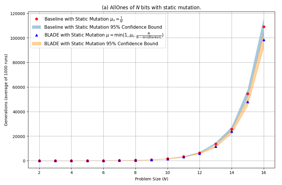
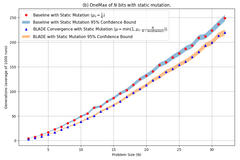
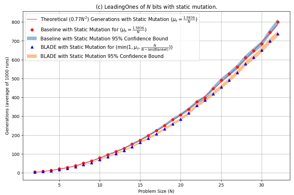
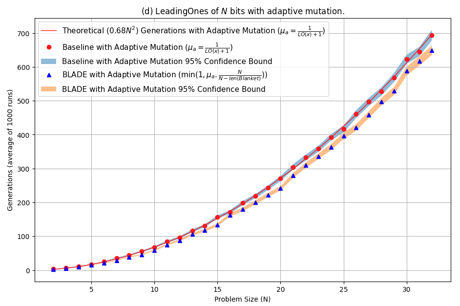
Figure 2. A comparison between the blanket method (i.e. BLADE on a single host) and the baseline method (i.e. standard evolution without blankets) across four benchmark problems: (a) AllOnes, (b) OneMax, and LeadingOnes with (c) static mutation and (d) adaptive mutation. The mutation rate for AllOnes and OneMax was $\mu_{=}\frac{1}{N}$. For LeadingOnes, the theoretically optimal mutation rates were used, i.e.  $\mu=\frac{1.5936}{N}$ in the static case and $\mu=\frac{1}{\mathrm{LO}(x)+1}$ in the adaptive case. The blanket method modifies these mutation rates by a factor of $\frac{N}{N-\mathrm{len(blanket)}}$ and clips them to one. The $x$-axis denotes the problem size $N$ (i.e. the length of the binary string) and the $y$-axis the average number of generations to converge, averaged over 1000 runs. The shaded areas indicate 95% confidence intervals. The results show that blankets improve convergence significantly on all problems.

4.2.1. AllOnes

Figure 2(a) illustrates the advantage of using blankets on AllOnes. Given that this is a needle-in-a-haystack problem, and the search space grows exponentially with string length, it is no surprise that the convergence time increases exponentially as well. However, BLADE converges slightly faster than the baseline, presumably due to the subdominant eigenvalues of the corresponding transition matrices. Further, as the problem size increase, the advantage of blankets becomes more pronounced.

4.2.2. OneMax

Figure 2(b) shows the advantage of using blankets on OneMax. BLADE converges significantly faster than the baseline, as indicated by a wide separation of the 95% confidence bounds, and the difference increases with problem size.

4.2.3. LeadingOnes

Figure 2(c) compares BLADE with the static mutation baseline and Figure 2(d) with the adaptive mutation baseline on LeadingOnes. Again, BLADE converges significantly faster than the baseline in both cases, and the advantage increases with problem size.

With the theoretically optimal mutation rate, the convergence rate with static mutation is $0.77N^{2}$, and with adaptive mutation is $0.68N^{2}$ (Papa and Doerr, 2020; Buzdalov and Doerr, 2020). These rates are plotted as continuous lines in Figures 2(c,d). As expected, they match the experimental results well.

4.3. Experiments With Distribution

The aim of these experiments is to study the contrast between just distributing the problem set and utilizing both blanket and distribution as BLADE does. Experiments were conducted for two, four, and eight clients and the results are depicted in Figure 3. A thorough discussion for each problem set is provided. In addition, a complete collection of these graphs can be found in A.1 for further examination.

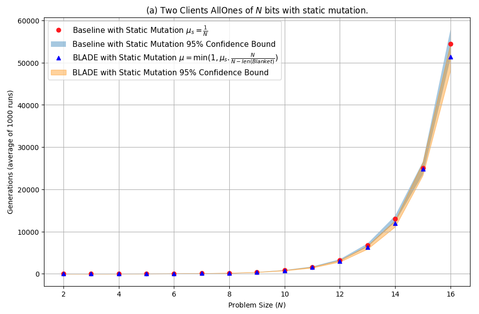
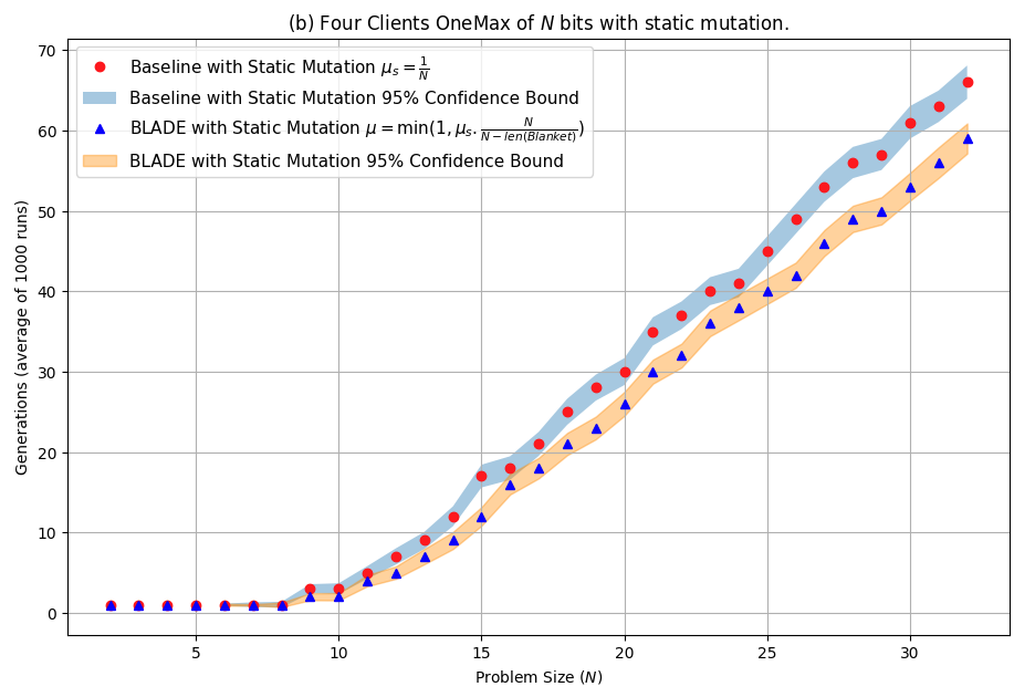
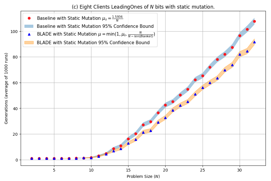
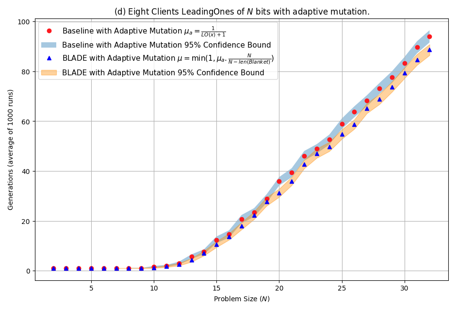
Figure 3. A comparison between full BLADE (including both blankets and distribution methods) and the baseline across the four benchmark problems. Representative results with two, four, and eight clients are shown; the complete set is included in Appendix A.1. The experimental and display details are the same as in Figure 2. The advantage of blankets extends to distribution across several clients: BLADE converges significantly faster than the baseline in all cases.

4.3.1. AllOnes

Figure 3(a) shows the advantage of using BLADE (combining distribution and masking) on AllOnes. The results are similar to the single client case: Both are exponential and BLADE is slightly better, with an increasing difference. Similar results were obtained in the four and eight-client cases.

4.3.2. OneMax

Figure 3(b) shows the advantage of BLADE on OneMax with distribution over four clients. Again, the results are similar to the single-client case, with BLADE converging significantly and increasingly faster than the baseline. Similar results were obtained in the two and eight-client cases.

4.3.3. LeadingOnes

Figures 3(c,d) compares BLADE with baseline on LeadingOnes distributed over eight clients. Again, BLADE converges significantly and increasingly faster than the baseline. Similar results were obtained in the two and four-client cases.

4.4. Synergy of Blankets and Distribution

Previous sections demonstrated that using blankets improves search performance over baseline both when it is run on a single client and when it is distributed over several clients. An interesting question is: Is there a synergy between blankets and distribution? That is, does distribution offer a larger speedup with BLADE than it does with the baseline?

To answer this question, the ratios of total evaluations in single-client and multi-client runs are plotted in Figure 4 for representative cases in each benchmark. A ratio of 1.0 means that the speedup is perfectly efficient, e.g. a run distributed over two clients converges twice as fast as a run on a single client. A ratio above one means that the threads provide additional information that the distribution algorithm can utilize to speed up the search even more.

A summary of these results is given below, and the comprehensive set of plots is included in Appendix  A.2.

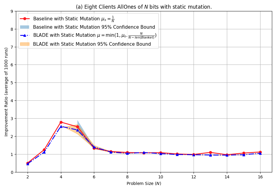
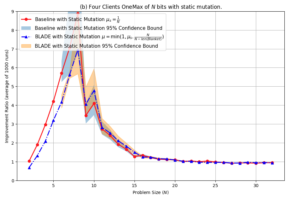
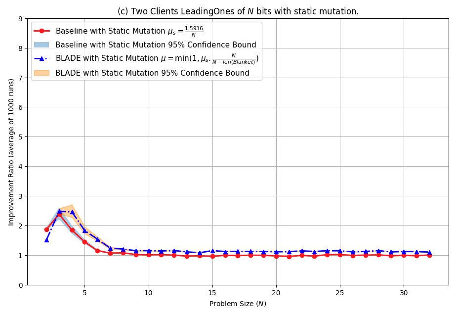
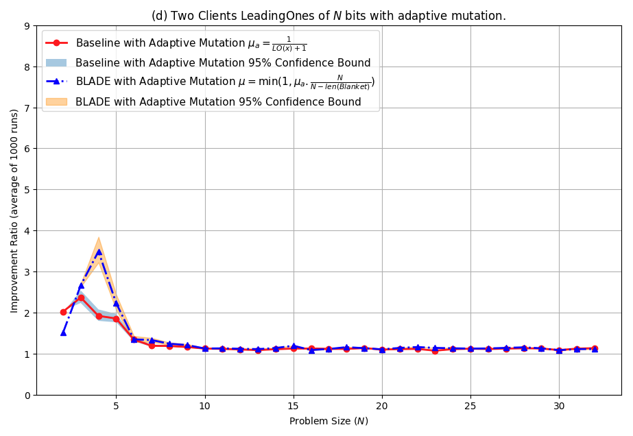
Figure 4. A comparison of the speedup ratio of BLADE vs. the baseline on the four benchmark problems. Similarly to Figure 3, representative results with two, four, and eight clients are shown; the complete set is included in Appendix A.2. A ratio of 1.0 indicates that the distribution is perfectly efficient, i.e. the total number of evaluations across all clients is the same as the number of evaluations on a single client. As the problem size grows, the ratio approaches 1.0 for AllOnes and OneMax. Remarkably, for LeadingOnes the ratio is above 1.0 for both the baseline and BLADE with adaptive mutation (d), and for BLADE only with static mutation (c). The results thus suggest that there is a synergy between adaptive mutation and distribution, and that BLADE provides the crucial adaptation in the otherwise static mutation case.

4.4.1. AllOnes

Figure 4(a) shows the improvement ratios in AllOnes when the runs are distributed over eight clients. When $N$ is small, there is a non-negligible chance that some of the clients have high-fitness individuals in their initial population, resulting in the high ratios up to $N=8$. With larger $N$, the ratios are close to one, suggesting that the distribution is efficient, and both the baseline and BLADE benefit from it equally. Similar results were obtained in the two and four-client cases.

4.4.2. OneMax

Figure  4(b) illustrates the improvement ratios in OneMax with a four-client distribution. The chance of having high-fitness individuals in the initial population is higher in this problem, and has a significant effect up to $N=20$. With larger $N$, the ratios are again close to one for both the baseline and BLADE, as in AllOnes. Similar results were obtained in the two and eight-client cases.

4.4.3. LeadingOnes

Figures 4(c,d) plots the improvement ratios in LeadingOnes with static and adaptive mutation with a two-client distribution. In this benchmark, the effect of lucky initialization is again small, and negligible after about $N=8$. With larger $N$, an interesting observation can be made: The improvement is significantly greater than one for BLADE in the static case, and for both the baseline and BLADE in the adaptive case. Similar results were obtained in the four and eight-client cases.

Apparently, in LeadingOnes there is information in the two threads that can be utilized to improve the search. This information can be captured to an extent through adaptive mutation; however, even when the mutation is static (as in Figure 4(c)), BLADE can still capture it. BLADE adjusts its mutation based on the blankets, and therefore establishes a version of the adaptive mutation process. This process allows it to take advantage of the synergy between threads more effectively than the baseline. Characterizing and optimizing this mechanism is a most exciting direction for future work.

5. Discussion and Future Work

BLADE can potentially be used to accelerate evolutionary algorithms by utilizing blanket-based tuning of search and by distributing the search. The experiments covered a wide range of fitness landscapes representative of many practical problems. The method is easily integrated as a plug-in into any preferred evolutionary method.

In order to put these conclusions into practice, there are two immediate directions for future work. The first is to extend the method from a $(1+1)EA$ to a population-based approach; the second is to generalize blankets to other evolutionary representations such as multi-dimensional vectors and trees. Once the BLADE method is extended in this manner, it can be tested in real-world applications. The goal will be to verify that more than $n$-fold speedup can be obtained with $n$ clients, taking advantage of the synergy between its two components.

Future theoretical research may seek to generalize the Markov chain approach to other problems and sizes. A particularly interesting challenge is to identify the conditions under which the synergy can emerge, and derive bounds for it. Such an understanding could be instrumental in developing faster evolutionary computation implementations in the future.

6. Conclusion

BLADE was demonstrated to accelerate a fundamental evolutionary algorithm in several benchmark problems. It can be easily integrated into other existing algorithms, making it possible to take advantage of it in practical applications. Its potential for providing more than $n$-fold speedup with $n$ clients is particularly intriguing and worthy of further study.

Appendix A Appendix: Comprehensive sets of graphs

A.1. Distribution Graphs

Figures 5, 6, and 7 show the results of the comparisons between BLADE and the baseline on the four benchmark problems with two, four, and eight clients, respectively.

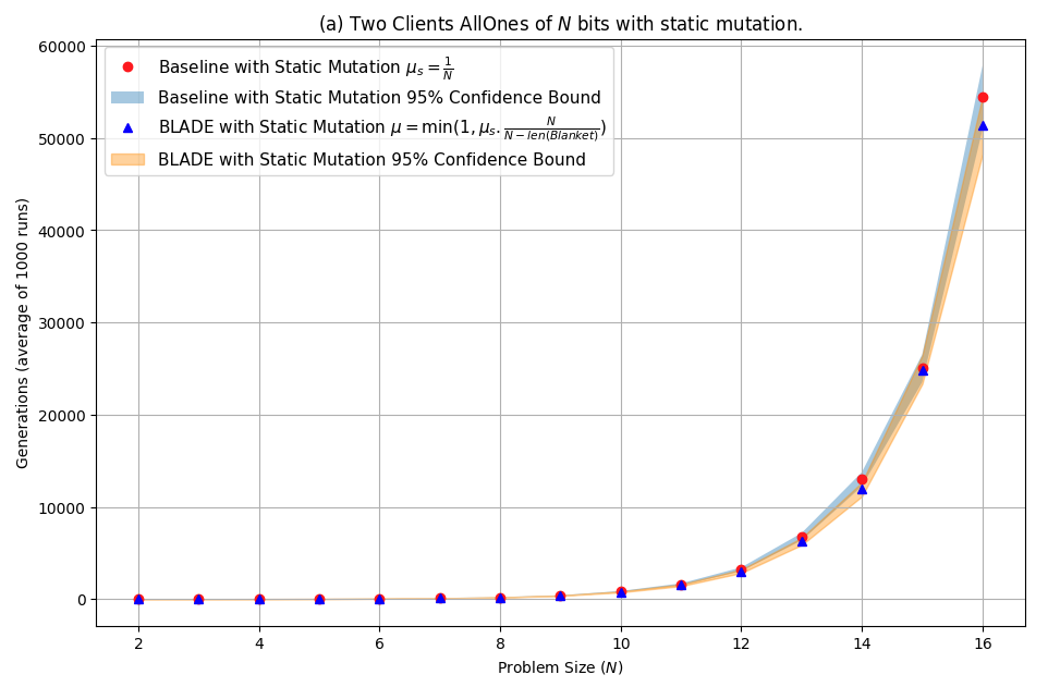
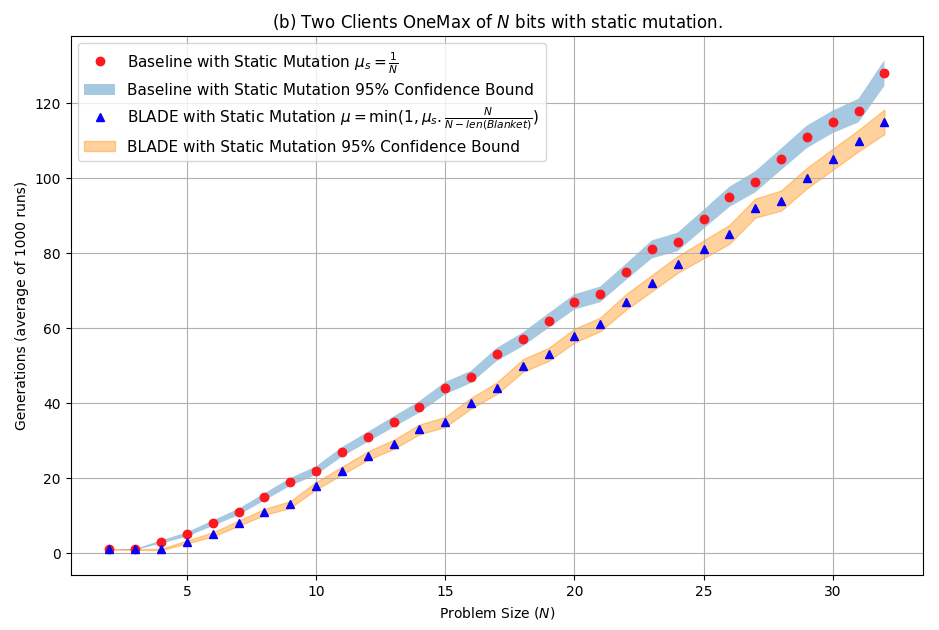
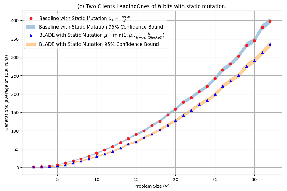
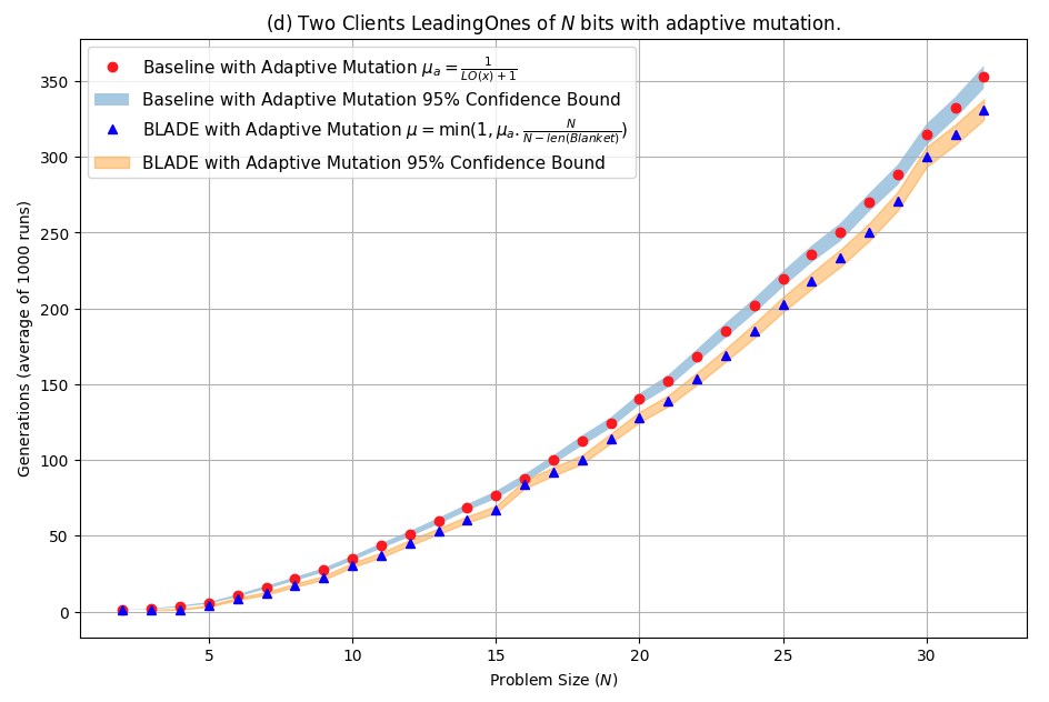
Figure 5. A comparison between BLADE and the baseline across the four benchmark problems with distribution over two clients; the experimental and display details are the same as in Figure 3. BLADE converges significantly faster than the baseline.

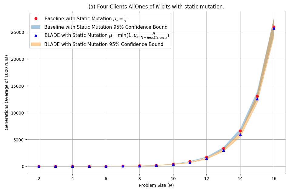
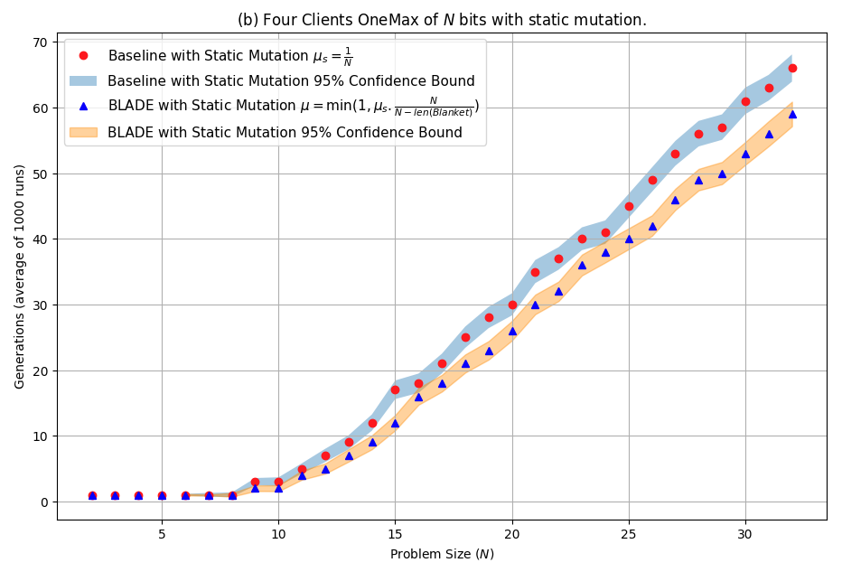
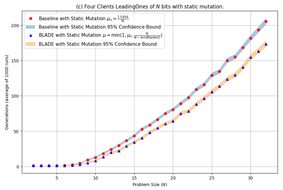
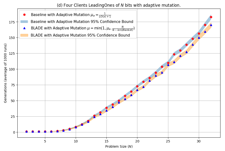
Figure 6. A comparison between BLADE and the baseline across the four benchmark problems with distribution over four clients; the experimental and display details are the same as in Figure 3. BLADE converges significantly faster than the baseline.

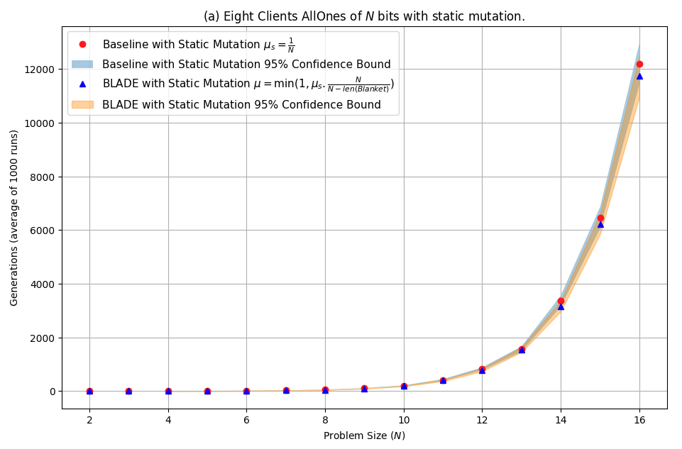
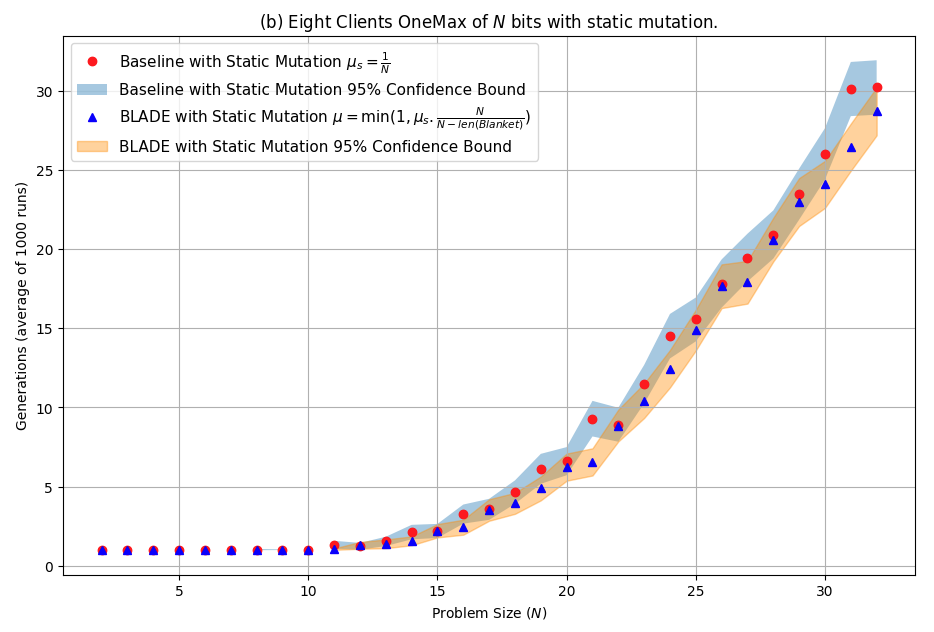
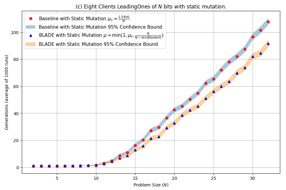
Figure 7. A comparison between BLADE and the baseline across the four benchmark problems with distribution over eight clients; the experimental and display details are the same as in Figure 3. BLADE converges significantly faster than the baseline.

A.2. Synergy Graphs

Figures 8, 9, and 10 compare the improvement ratios of BLADE and the baseline on the four benchmark problems with two, four, and eight clients, respectively.

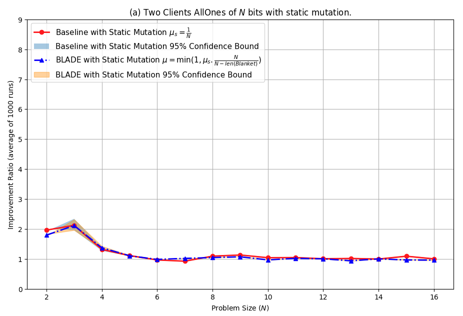
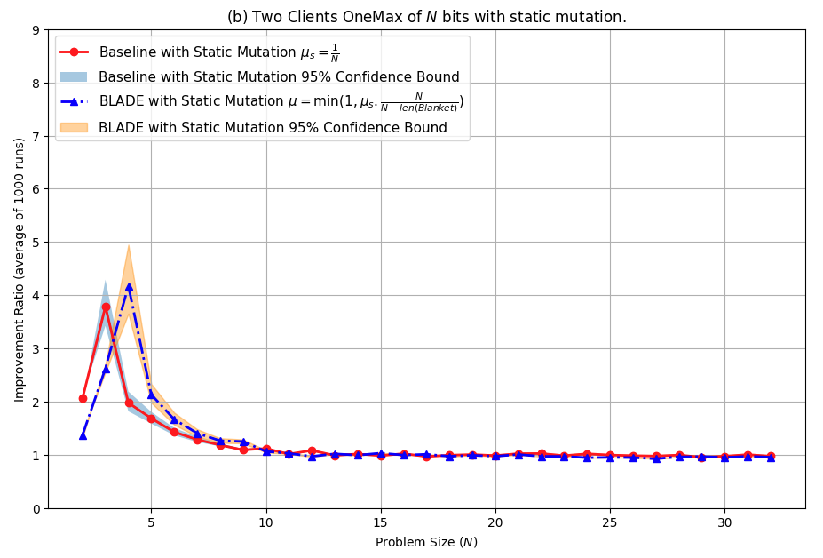
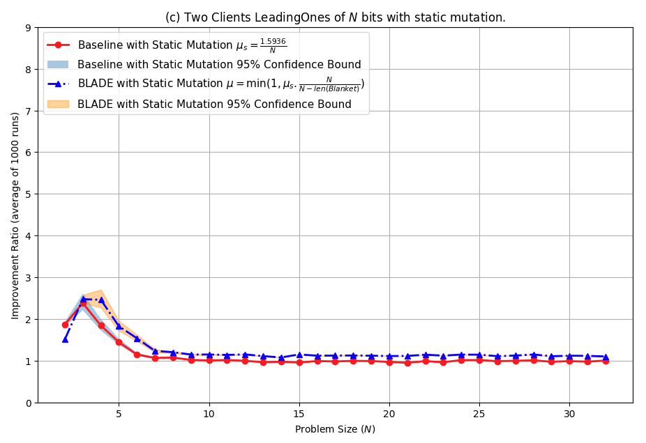
Figure 8. A comparison of the speedup ratio of BLADE vs. the baseline on the four benchmark problems with distribution over two clients; the experimental and display details and conclusions are similar to those in Figure 4.

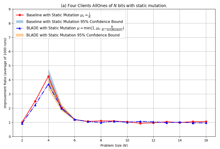
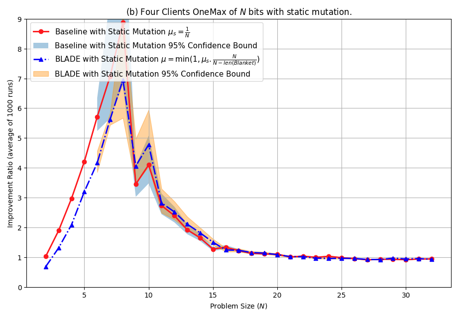
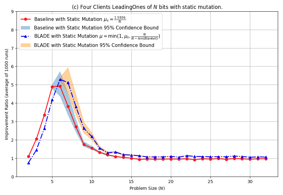
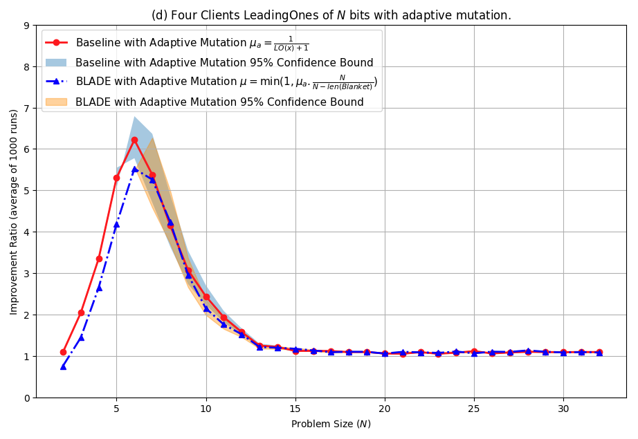
Figure 9. A comparison of the speedup ratio of BLADE vs. the baseline on the four benchmark problems with distribution over four clients; the experimental and display details and conclusions are similar to those in Figure 4.

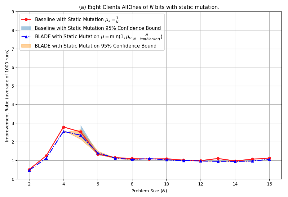
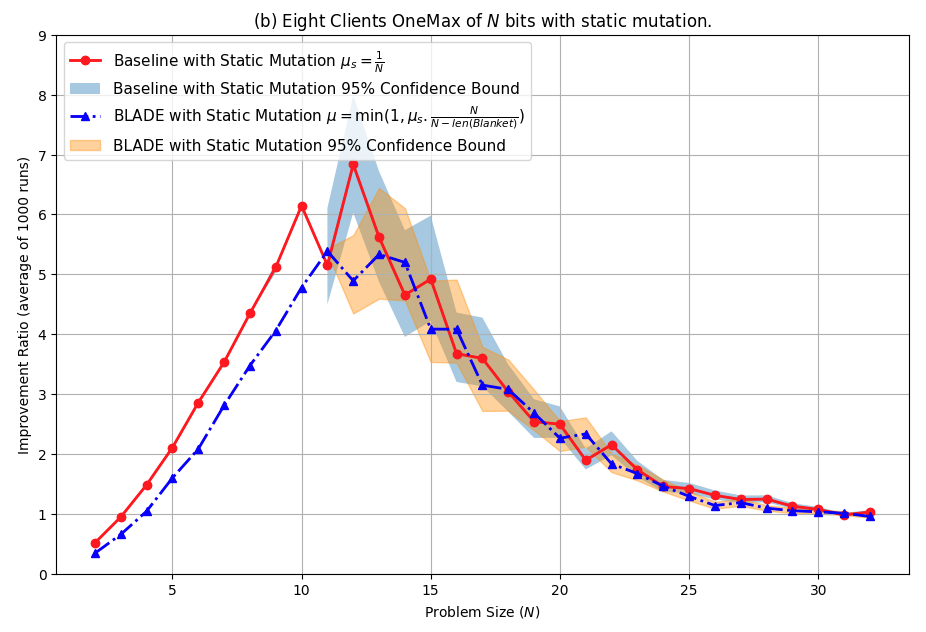
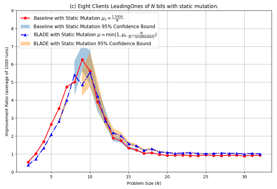
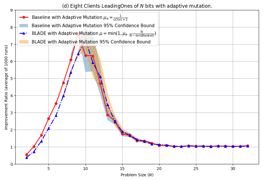
Figure 10. A comparison of the speedup ratio of BLADE vs. the baseline on the four benchmark problems with distribution over eight clients; the experimental and display details and conclusions are similar to those in Figure 4.

References

- (1)
- Ansótegui et al. (2009) Carlos Ansótegui, Meinolf Sellmann, and Kevin Tierney. 2009. A gender-based genetic algorithm for the automatic configuration of algorithms. In Principles and Practice of Constraint Programming-CP 2009: 15th International Conference, CP 2009 Lisbon, Portugal, September 20-24, 2009 Proceedings 15. Springer, 142–157.
- Berman and Plemmons (1994) Abraham Berman and Robert J Plemmons. 1994. Nonnegative matrices in the mathematical sciences. SIAM.
- Buskulic and Doerr (2019) Nathan Buskulic and Carola Doerr. 2019. Maximizing Drift is Not Optimal for Solving OneMax. In Proceedings of the Genetic and Evolutionary Computation Conference Companion (Prague, Czech Republic) (GECCO ’19). Association for Computing Machinery, New York, NY, USA, 425–426. https://doi.org/10.1145/3319619.3321952
- Buzdalov and Doerr (2020) Maxim Buzdalov and Carola Doerr. 2020. Optimal Mutation Rates for the EA on OneMax. In Parallel Problem Solving from Nature – PPSN XVI: 16th International Conference, PPSN 2020, Leiden, The Netherlands, September 5-9, 2020, Proceedings, Part II (Leiden, The Netherlands). Springer-Verlag, Berlin, Heidelberg, 574–587. https://doi.org/10.1007/978-3-030-58115-2_40
- Doerr et al. (2019) Carola Doerr, Furong Ye, Naama Horesh, Hao Wang, Ofer M. Shir, and Thomas Bäck. 2019. Benchmarking Discrete Optimization Heuristics with IOHprofiler. In Proceedings of the Genetic and Evolutionary Computation Conference Companion (Prague, Czech Republic) (GECCO ’19). Association for Computing Machinery, New York, NY, USA, 1798–1806. https://doi.org/10.1145/3319619.3326810
- Droste et al. (2002) Stefan Droste, T. Jansen, and Ingo Wegener. 2002. On the analysis of the (1+1) evolutionary algorithm. Theor. Comput. Sci. 276 (2002), 51–81.
- Elsken et al. (2019) Thomas Elsken, Jan Hendrik Metzen, and Frank Hutter. 2019. Neural Architecture Search: A Survey. Journal of Machine Learning Research 20 (2019), 1–21. http://www.jmlr.org/papers/volume20/18-598/18-598.pdf
- Gagniuc (2017) Paul A. Gagniuc. 2017. Markov Chains: From Theory to Implementation and Experimentation.
- Gerules and Janikow (2016) G. Gerules and C. Janikow. 2016. A survey of modularity in genetic programming. In 2016 IEEE Congress on Evolutionary Computation (CEC). 5034–5043.
- Gomez et al. (2008) Faustino Gomez, Jürgen Schmidhuber, and Risto Miikkulainen. 2008. Accelerated Neural Evolution Through Cooperatively Coevolved Synapses. Journal of Machine Learning Research 9 (2008), 937–965.
- Hassanat et al. (2019) Ahmad Hassanat, Khalid Almohammadi, Esra’a Alkafaween, Eman Abunawas, Awni Hammouri, and V. B. Surya Prasath. 2019. Choosing Mutation and Crossover Ratios for Genetic Algorithms—A Review with a New Dynamic Approach. Information 10, 12 (2019). https://doi.org/10.3390/info10120390
- Hassani and Treijs (2009) Abtin Hassani and Jonatan Treijs. 2009. An Overview of Standard and Parallel Genetic Algorithms.
- Kirkland (2009) Steve Kirkland. 2009. Subdominant Eigenvalues for Stochastic Matrices with Given Column Sums. Electronic Journal of Linear Algebra 18 (2009), 57.
- Lässig and Sudholt (2014) Jörg Lässig and Dirk Sudholt. 2014. General Upper Bounds on the Runtime of Parallel Evolutionary Algorithms*. Evolutionary Computation 22 (2014), 405–437.
- Liang et al. (2021) Jason Liang, Santiago Gonzalez, Hormoz Shahrzad, and Risto Miikkulainen. 2021. Regularized Evolutionary Population-Based Training. In Proceedings of the Genetic and Evolutionary Computation Conference. http://nn.cs.utexas.edu/?liang:gecco21
- Liang et al. (2019) Jason Liang, Elliot Meyerson, Babak Hodjat, Dan Fink, Karl Mutch, and Risto Miikkulainen. 2019. Evolutionary Neural AutoML for Deep Learning. In Proceedings of the Genetic and Evolutionary Computation Conference (GECCO-2019). http://nn.cs.utexas.edu/?liang:gecco19
- Liang and Miikkulainen (2015) Jason Zhi Liang and Risto Miikkulainen. 2015. Evolutionary Bilevel Optimization for Complex Control Tasks. In Proceedings of the Genetic and Evolutionary Computation Conference (GECCO 2015). Madrid, Spain. http://nn.cs.utexas.edu/?liang:gecco2015
- Martinez et al. (2019) Ruben Martinez, J. C. Puche, Frank Delgado, and J. Finat. 2019. Evolutionary Algorithms: Multimodal Problems and Spatial Distribution.
- Miikkulainen et al. (2020) Risto Miikkulainen, Jason Liang, Elliot Meyerson, Aditya Rawal, Dan Fink, Olivier Francon, Bala Raju, Hormoz Shahrzad, Arshak Navruzyan, Nigel Duffy, and Babak Hodjat. 2020. Evolving Deep Neural Networks. In Artificial Intelligence in the Age of Neural Networks and Brain Computing, C. F. Morabito, C. Alippi, Y. Choe, and R. Kozma (Eds.). Elsevier, New York.
- Moriarty and Miikkulainen (1997) David E. Moriarty and Risto Miikkulainen. 1997. Forming Neural Networks Through Efficient and Adaptive Co-Evolution. Evolutionary Computation 5 (1997), 373–399.
- O’Reilly et al. (2013) Una-May O’Reilly, Mark Wagy, and Babak Hodjat. 2013. EC-Star: A Massive-Scale, Hub and Spoke, Distributed Genetic Programming System. Springer New York, New York, NY, 73–85. https://doi.org/10.1007/978-1-4614-6846-2_6
- Papa and Doerr (2020) Gregor Papa and Carola Doerr. 2020. Dynamic control parameter choices in evolutionary computation: GECCO 2020 tutorial. 927–956. https://doi.org/10.1145/3377929.3389876
- Potter and Jong (2000) Mitchell A. Potter and Kenneth A. De Jong. 2000. Cooperative Coevolution: An Architecture for Evolving Coadapted Subcomponents. Evolutionary Computation 8 (2000), 1–29.
- Raghul and Jeyakumar (2021) S. Raghul and G. Jeyakumar. 2021. Parallel and Distributed Computing Approaches for Evolutionary Algorithms—A Review. Advances in Intelligent Systems and Computing (2021).
- Rowe and Sudholt (2012) Jonathan E. Rowe and Dirk Sudholt. 2012. The choice of the offspring population size in the (1,) EA. In Annual Conference on Genetic and Evolutionary Computation.
- Seneta (2008) Eugene Seneta. 2008. Non-negative Matrices and Markov Chains.
- Sinha et al. (2014) Ankur Sinha, Pekka Malo, Peng Xu, and Kalyanmoy Deb. 2014. A bilevel optimization approach to automated parameter tuning. In Proceedings of the Genetic and Evolutionary Computation Conference (GECCO 2014). Vancouver, BC, Canada.
- Strasser et al. (2017) Shane Strasser, John W. Sheppard, Nathan Fortier, and Rollie Goodman. 2017. Factored Evolutionary Algorithms. IEEE Transactions on Evolutionary Computation 21 (2017), 281–293.
- Stützle et al. (2022) Thomas Stützle, Manuel López-Ibáñez, and Leslie Pérez-Cáceres. 2022. Automated Algorithm Configuration and Design. In Proceedings of the Genetic and Evolutionary Computation Conference Companion (Boston, Massachusetts) (GECCO ’22). Association for Computing Machinery, New York, NY, USA, 997–1019. https://doi.org/10.1145/3520304.3533663
- Sudholt (2015) Dirk Sudholt. 2015. Parallel Evolutionary Algorithms. In Handbook of Computational Intelligence.
- Tuson and Ross (1998) Andrew Tuson and Peter Ross. 1998. Adapting Operator Settings in Genetic Algorithms. Evolutionary Computation 6, 2 (06 1998), 161–184. https://doi.org/10.1162/evco.1998.6.2.161 arXiv:https://direct.mit.edu/evco/article-pdf/6/2/161/1493027/evco.1998.6.2.161.pdf
- Vaswani et al. (2017) Ashish Vaswani, Noam Shazeer, Niki Parmar, Jakob Uszkoreit, Llion Jones, Aidan N Gomez, Ł ukasz Kaiser, and Illia Polosukhin. 2017. Attention is All you Need. In Advances in Neural Information Processing Systems, I. Guyon, U. Von Luxburg, S. Bengio, H. Wallach, R. Fergus, S. Vishwanathan, and R. Garnett (Eds.), Vol. 30. Curran Associates, Inc.
- Whitley et al. (1998) Darrell Whitley, Soraya Rana, and Robert Heckendorn. 1998. The Island Model Genetic Algorithm: On Separability, Population Size and Convergence. Journal of Computing and Information Technology 7 (12 1998).
- Yang et al. (2019) Peng Yang, Ke Tang, and Xin Yao. 2019. A Parallel Divide-and-Conquer-Based Evolutionary Algorithm for Large-Scale Optimization. IEEE Access 7 (2019), 163105–163118. https://doi.org/10.1109/ACCESS.2019.2938765