Boosted ab initio Cryo-EM 3D Reconstruction with ACE-EM

Abstract

The central problem in cryo-electron microscopy (cryo-EM) is to recover the 3D structure from noisy 2D projection images which requires estimating the missing projection angles (poses). Recent methods attempted to solve the 3D reconstruction problem with the autoencoder architecture, which suffers from the latent vector space sampling problem and frequently produces suboptimal pose inferences and inferior 3D reconstructions. Here we present an improved autoencoder architecture called ACE (Asymmetric Complementary autoEncoder), based on which we designed the ACE-EM method for cryo-EM 3D reconstructions. Compared to previous methods, ACE-EM reached higher pose space coverage within the same training time and boosted the reconstruction performance regardless of the choice of decoders. With this method, the Nyquist resolution (highest possible resolution) was reached for 3D reconstructions of both simulated and experimental cryo-EM datasets. Furthermore, ACE-EM is the only amortized inference method that reached the Nyquist resolution.

1 Introduction

Single-particle cryo-electron microscopy (cryo-EM) is one of the most important structural biology techniques  [1]. This technique can be divided into four stages: biological sample preparation, electron microscopy image collection, 3-dimensional (3D) reconstruction, and atomic structural model building. 3D reconstruction of molecular volumes from 2-dimensional (2D) electron microscopy images is the most challenging and time-consuming step in cryo-EM data analysis. There are two major challenges in cryo-EM 3D reconstruction: unknown projection poses (orientations and positions) and low signal-to-noise ratio (SNR). During electron microscopy imaging, the 3D poses of the biological molecules in the sample can not be directly measured. The SNR of a typical cryo-EM image is very low, which can vary from -10 dB to -20 dB (average around -10 dB)  [2], making it extremely challenging to accurately estimate poses and perform the 3D reconstruction.

Currently, many machine-learning (ML)-based methods have been proposed for solving cryo-EM 3D reconstruction  [3], utilizing architectures like GAN  [4] and auto-encoders  [5]. Nevertheless, ML-based methods of cryo-EM 3D reconstruction are still at an early stage. The highest possible cryo-EM reconstruction resolution (2 pixels) at FSC threshold 0.5 has not been achieved by ML-based methods, even in simulated datasets without noise. For experimental datasets like the 80S, some methods with amortized inference methods failed to reconstruct the object of certain size, or found the highest possible resolution (2 pixels) of half-map FSC  [6] at 0.143 not reachable  [7]. For widely utilized architecture auto-encoders, an image-to-pose encoder extracts the image-projection poses from 2D input cryo-EM images, while a pose-to-image decoder generates the images to match the inputs. However, as the poses are intermediate latent variables without supervised loss, the estimated poses can be inaccurate and easily trapped in local minima of the orientation space. These pose estimation errors lead to an inferior resolution in the 3D reconstruction output.

To improve the pose estimation and 3D reconstruction quality, here we propose a new framework called ACE-EM (ACE for Asymmetric Complementary autoEncoder). In particular, ACE-EM consists of two training tasks: (1) Image-pose-image (IPI). The task is the same as previous work, which takes projection images as inputs, and outputs predicted images, by an image-to-pose encoder followed by a pose-to-image decoder. (2) Pose-image-pose (PIP). The task explicitly learns the pose estimation in a self-supervised fashion, which takes randomly sampled poses as inputs, and outputs predicted poses, using the same encoder and decoder as in IPI but reversing their order. The two tasks complement each other and achieve a more balanced training of the autoencoder parameters.

Our main contributions are listed below.

• As far as we know, ACE-EM is the first deep-learning model in cryo-EM reconstruction that enhances the pose estimation by the self-supervised PIP task. With better pose estimation, ACE-EM can converge much faster than previous methods, efficiently cover more pose spaces, and achieve better cryo-EM 3D reconstruction quality.

• ACE-EM can boost performance regardless of decoder types. For example, some decoders, that failed in previous autoencoder architectures, can be successfully used in ACE-EM.

• Experimental results demonstrate that ACE-EM can perform well in both simulated and real-world experimental datasets. In particular, ACE-EM outperformed all the baseline methods and reached 2 pixels, the Nyquist resolution (the highest possible resolution) at FSC threshold 0.5, the Nyquist resolution of half-map FSC at 0.143 in the 80S experimental dataset, which is the only architecture that reached the Nyquist resolution with amortized inference methods.

2 Related work

Overview of cryo-EM methods

3D reconstruction and view synthesis is a popular field in computer vision. Many new methods have been emerged in recent years, such as NeRF  [8], Plenoxels  [9], DirectVoxGo  [10], BARF  [11], SCNeRF  [12], and GNeRF  [12]. These methods can reconstruct 3D scenes from natural images with high signal-to-noise ratios (SNR). In ab initio cryo-EM 3D reconstruction, the reconstruction problem is much harder due to the low-SNR nature of cryo-EM images and missing image projection parameters. In addition to traditional cryo-EM reconstruction methods like RELION  [13] and cryoSPARC  [14], many ML-based cryo-EM reconstruction methods have been developed in the past few years. Given only the 2D cryo-EM projection images without any labels, cryo-EM 3D reconstruction can be formulated as a self-supervised learning problem. Two ML frameworks have been explored: GAN  [4] and autoencoder  [5]. CryoGAN  [15] and Multi-CryoGAN  [16] adopted the GAN framework. In these methods, the generator contains the predicted volume information and generates projection images, while the discriminator adopts the generated and authentic images and discriminates the source of the images. However, due to the limitations of GANs, these methods lack pose estimation and 3D reconstruction quality is inferior to other methods. For cryo-EM, the images are fed to the encoder to generate a latent variable (usually representing the pose estimation), and the decoder produces the reconstructed images based on this variable. The model is trained by reducing the loss of the original and reconstructed ones. After training, the 3D reconstruction density map can be obtained from the decoder. Cryo-EM 3D reconstruction with variational autoencoder (VAE)  [17], CryoDRGN  [18, 19, 20], AtomVAE  [21], CryoPoseNet  [22], and cryoAI  [7] adopt the autoencoder architecture. They improve the performance of autoencoders in cryo-EM 3D reconstructions by using more powerful networks for encoders and decoders, adding or modifying loss functions, modifying the latent variable designs and other strategies.

Pose estimation

Pose estimation is concerned with estimating the missing orientation and position (together known as pose) parameters of the images based on the underlying 3D object. Existing pose estimation methods can be divided into two classes: Per-image pose search methods and amortized inference methods. The first class of methods performs a global pose search for each projection image in the input dataset. Traditional software, like RELION  [13] and cryoSPARC  [14], and some ML-based methods, inluding cryoDRGN-BNB [18] and CryoDRGN2 [20], fall into this category. The per-image pose search method is not an ML-based strategy, To control the Pose estimation as an ML process, the second class method, amortized inference, is first proposed for cryo-EM 3D reconstruction by Ullrich et. al.  [17]. It focuses on learning a parameterized function for mapping image $Y_{i}$ to its pose $\phi_{i}$, then it is widely accepted by autoencoder solutions as the encoder. For autoencoders with amortized inference method, they suffer from too many local minima in their probabilistic pose estimation framework. Rosenbaum et. al. attempted to overcome local-minima traps using variational autoencoder (VAE)  [23]. CryoAI  [7] extended CryoPoseNet  [22] work by introducing “symmetry loss” to facilitate pose learning by adding a 180^∘-rotated input image as input. In practice, we found these strategies are insufficient for avoiding poses being trapped in local minima. The proposed ACE-EM method also falls into this category of amortized inference.

Decoder or generator choices

In the view of cryo-EM 3D reconstruction, a decoder (in autoencoder) or a generator (in GAN) is a structure that contains the volume representation, which adopts the pose or other variables and outputs the predicted 2D projection images. The underlying target 3D object can have either real-space or frequency-space representations in the space domain, and either neural network type or voxel grid type for volume parameter representations  [3]. Traditional softwares represent the reconstruction target volume as a 3D voxel grid of frequency space, like Relion  [13] and cryoSPARC  [14]. Many recently developed deep-learning-based reconstruction methods mainly use two types of decoders (generators): real-space voxel grid type and frequency-space neural network type. CryoDRGN  [18, 19, 20] and CryoAI  [7] uses the frequency-space neural network as their decoders. Real-space voxel grid methods are also used by many algorithms, such as CryoGAN  [15], Multi-CryoGAN  [16], 3DFlex  [24], and AtomVAE  [21]. CryoPoseNet  [22] stores a real space voxel grid representation of the reconstruction target, but the projection was made in Fourier space. In this work, we show that the ACE-EM method is effective with both real-space voxel grid type and frequency-space neural network type of decoders.

Cyclic training

Our method uses encoder-decoder(E-D) and decoder-encoder(D-E) two orders for training in autoencoders, and this cyclic training is widely used in style transfer, like MUNIT  [25], DRIT  [26] and CDD  [27]. These methods differ from ours in 4 main aspects, architecture setting, data format, aims, and challenges. For the architecture setting, MUNIT uses E-D and (E-)D-E two orders  [25], DRIT uses one task E-D-E-D to finish the cycle, while more complex tasks are used in CDD. MUNIT and DRIT need two random images inputted together as a group for cross-domain translation  [26, 27], CDD uses paired data for supervised learning  [27], but paired or grouped data is not required by ACE-EM. Style transfer aims to decouple images’ style and content, and our aim is to settle the poses in an accurate distribution. Also, our methods face specific reconstruction challenges, like noise problems.

3 Approach

3.1 Overview of ACE-EM

ACE-EM is an autoencoder-based model and is trained with two unsupervised learning tasks. The autoencoder contains an image-to-pose encoder ($E_{IP}$) and a pose-to-image decoder ($D_{PI}$). The $E_{IP}$ takes projection images and outputs projection pose parameters. The $D_{PI}$ can be viewed as a cryo-EM image projection physics simulator. It takes the pose parameters and outputs projection images corresponding to the given poses, which are post-processed by applying CTF  [28]. The first task of ACE-EM is image-pose-image(IPI) task which follows the standard unsupervised autoencoder architecture. With the pipeline of $E_{IP}$ and $D_{PI}$, reconstructed images are generated corresponding to the given projection images. The second task is the pose-image-pose (PIP) task, a self-supervised learning, that uses the same encoder-decoder in IPI but in the reversed order. With the reverse pipeline, a corresponding pose is predicted from a random-selected pose, and the gap between the two poses is minimized in training. The IPI task and PIP task can be trained simultaneously or in alternating steps. With either training strategy, the $E_{IP}$ and $D_{PI}$ parameters are shared between the two tasks. As a result, the two tasks of ACE-EM complement each other and form a more balanced training of the $E_{IP}$ and $D_{PI}$ parameters.

Figure 1: The network architecture of ACE-EM. The IPI task is shown at the top highlighted in blue, while the PIP task is shown at the bottom highlighted in salmon.

3.2 Encoder $E_{IP}$ and Decoder $D_{PI}$

The $E_{IP}$ represents a function that maps an input image $Y_{i}$ to its corresponding projection pose parameters $(R_{i},t_{i})$. $R_{i}\in SO(3)\subset\mathbb{R}^{3\times 3}$ is a rotation matrix for mapping a reference orientation to the projection orientation. $t_{i}\in\mathbb{R}^{2}$ is the 2D translation vector to account for the 2D image shift in the input image $Y_{i}$. The $D_{PI}$ takes pose $(R_{i},t_{i})$ and predicts the projection image $Y_{i}^{pred}$.The trainable parameters of $D_{PI}$ contain the cryo-EM volume in an explicit or implicit way, and the volume can be obtained from the $D_{PI}$ after training. CTF was applied to the output images to create a more realistic projection image $Y_{i}^{pred}$. The details of the encoder and decoder structure can be found in appendix A.

$$E_{IP}:Y_{i}\mapsto(R_{i},t_{i})$$ (1)

$$D_{PI}:(R_{i},t_{i})\mapsto Y_{i}^{pred}$$ (2)

Choices of decoders

ACE-EM provides an architecture that can work with different encoders and decoders. Cryo-EM 3D reconstruction can have either real-space or frequency-space representations in the space domain, and either neural network type or voxel grid type for volume parameter representations. To prove ACE-EM is universal and can boost the performances regardless of the decoder types, we tested a real-space voxel grid decoder $\mathrm{VoxelGrid_{R}}$ which was used in cryoGAN  [15], and partially used in the CryoPoseNet  [22], and a frequency-space neural network decoder $\mathrm{FourierNet}$ which was shown to outperform other similar methods   [7].

3.3 IPI (Image-Pose-Image) task

The IPI task follows the standard autoencoder architecture as shown in Figure 1. Using the notations defined earlier, the IPI task can be formally defined as follows.

$$\text{IPI}:Y_{i}\mapsto Y_{i}^{pred}$$ (3)

$$f_{IPI}(Y_{i}):=(D_{PI}\circ E_{IP})(Y_{i})$$ (4)

IPI loss function

Since both the input and output are images, the objective of the IPI task is to minimize their differences by mean squared error (MSE) loss function for each training batch of size $B$ and with an image edge length of $L$.

$$\mathcal{L}_{image}:=\frac{1}{BL^{2}}\sum_{i=1}^{B}\left\|Y_{i}-Y_{i}^{pred}\right\|_{2}$$ (5)

Cryo-EM 3D reconstruction is prone to spurious 2-fold planar mirror symmetry  [7]. A tentative solution is to use the “symmetric loss" employed in cryoAI  [7], where $\Gamma_{\text{cryoAI}}$ is the cryo-AI autoencoder pipeline and $R_{\pi}$ represents an in-plane rotation of angle $\pi$ operation applied to the input image $Y_{i}$.

$$\mathcal{L}_{\text{symm}}^{\text{cryoAI}}:=\frac{1}{BL^{2}}\sum_{i=1}^{B}\min(\left\|Y_{i}-\Gamma_{\text{cryoAI}}(Y_{i})\right\|_{2},\left\|R_{\pi}[Y_{i}]-\Gamma_{\text{cryoAI}}(R_{\pi}[Y_{i}])\right\|_{2})$$ (6)

For a consideration of data augmentation, we have generalized the above symmetric loss to include in-plane image rotation by arbitrary angles and also included mirror transformation. “generalized symmetric loss" as below. $A_{1}[Y_{i}]$ and $A_{2}[Y_{i}]$ are two different affine transformations with random image rotations and/or mirror flipping. We found that the generalized symmetry loss still works with the voxel-grid-based decoder $\mathrm{VoxelGrid_{R}}$, but fails in $\mathrm{FourierNet}$, so it is only applied when using the $\mathrm{VoxelGrid_{R}}$.

$$\mathcal{L}_{\text{symm}}^{G}:=\frac{1}{BL^{2}}\sum_{i=1}^{B}\min(\left\|A_{1}[Y_{i}]-f_{IPI}(A_{1}[Y_{i}])\right\|_{2},\left\|A_{2}[Y_{i}]-f_{IPI}(A_{2}[Y_{i}])\right\|_{2})$$ (7)

In addition to image loss, we also added an L1-regularization term for image shift to avoid unrealistic large shift predictions and keep the reconstructed 3D object near the origin of the coordinate system.

$$\mathcal{L}_{IPI}:=\mathcal{L}_{\text{symm}}^{G}+\frac{1}{2B}\sum_{i=1}^{B}\left\|t_{i}^{pred}\right\|_{1}$$ (8)

IPI warm-up labeling

High-frequency features are difficult to learn in at an early training stage, especially for projection images with low SNR. We found that the training results can be improved by using the low-pass filtered input images as training labels instead of using original image labels, as a training warm-up. The training image label ${\tilde{Y_{i}}}$ is defined below. The details of $f_{\text{filter-k}}$ can be found in appendix A. $f_{\text{filter-1}}$ is the first Gaussian filter with the lowest Gaussian convolution kernel variance, while $f_{\text{filter-k}}$ is the k-th Gaussian filter with higher convolution kernel variance. $N_{\text{warm-up}}^{IPI}$ is the iteration threshold for switching to the original input images. In practice, 3, 4 or 5 is selected as $k$ value.

$$\tilde{Y_{i}}=\gamma(Y_{i})+(1-\gamma)f_{\text{filter-k}}(Y_{i})$$ (9)

$$\gamma=\begin{cases}0,&\text{if iteration}\,<N_{\text{warm-up}}^{IPI}\\ 1,&\text{if iteration}\,>=N_{\text{warm-up}}^{IPI}\\ \end{cases}$$ (10)

3.4 PIP (Pose-Image-Pose) task

The PIP task is similar to the IPI task but with $E_{IP}$ and $D_{PI}$ placed in reverse order. Besides, an additive Gaussian noise $\epsilon\sim\mathcal{N}(\mu,\sigma^{2}I)$ is added to the output image from $D_{PI}$ to create more realistic inputs for the $E_{IP}$. The $\mu$ and $\sigma$ of the Gaussian noise is sampled based on the background of the input images or on a given SNR. Compared to the IPI task, the inputs of PIP have changed from images to synthesized projection parameters $(R_{i},t_{i})$ drawn from certain distributions. The loss function is defined as the MSE loss of rotation matrices $\{R_{i}\}_{i\in{\mathcal{B}}}$ and translation vectors $\{t_{i}\}_{i\in\mathcal{B}}$ for each batch $\mathcal{B}$ of size $B$ as shown below, where $\left\|\cdot\right\|_{F}$ is the Frobenius matrix norm.

$$PIP:(R_{i}^{syn},t_{i}^{syn})\mapsto(R_{i}^{pred},t_{i}^{pred})$$ (11)

$$f_{PIP}(R_{i}^{syn},t_{i}^{syn}):=E_{IP}(D_{PI}(R_{i}^{syn},t_{i}^{syn})+\epsilon)$$ (12)

$$\mathcal{L}_{PIP}=\frac{1}{B}\sum_{i=1}^{B}(\frac{1}{9}\left\|R_{i}^{syn}-R_{i}^{pred}\right\|_{2}+\frac{1}{2}\left\|t_{i}^{syn}-t_{i}^{pred}\right\|_{1})$$ (13)

With only IPI, the pose estimation of $E_{IP}$ is not distributed in the whole pose space, and some part of the pose space is never reached. By applying PIP, in which the input pose is randomly sampled in the whole pose space, $E_{IP}$ is forced to match the image-pose pairs over all possible pose spaces. Therefore, PIP gives $E_{IP}$ a proper output distribution and lets the model measure infinity of pose and images instead of only images in datasets. With a substantially correct volume representation of $D_{PI}$, PIP even turns the unsupervised task into a supervised image-pose matching task. When training the PIP task, one has the choice of freezing the $D_{PI}$ parameters and only training the $E_{IP}$, or allowing both the $E_{IP}$ and $D_{PI}$ parameters to be updated.

3.5 Training of the IPI and PIP tasks

The IPI and PIP tasks can be trained together or in succession. When trained together, we designed the following training schedule with a warm-up period of $N_{\text{warm-up}}^{\text{train}}$ iterations, which allows the IPI task to learn an approximate description of the underlying 3D object before adding the PIP task. Although we found the following simple schedule was sufficient in our benchmark tests, other schedules of $\beta$ are also possible.

$$\mathcal{L}_{total}=\mathcal{L}_{IPI}+\beta\mathcal{L}_{PIP}$$ (14)

$$\begin{cases}\beta=0,&\text{if iteration}\,<N_{\text{warm-up}}^{\text{train}}\\ \beta>0,&\text{if iteration}\,>=N_{\text{warm-up}}^{\text{train}}\\ \end{cases}$$ (15)

4 Results

To evaluate the ab initio 3D reconstruction quality of ACE-EM, we benchmarked this method against both the traditional cryo-EM 3D reconstruction software cryoSPARC  [14] and recent methods, including cryoPoseNet  [22], cryoDRGN2  [20], and cryoAI  [7], on both simulated and experimental cryo-EM datasets.

4.1 Dataset Preparation and Training Setup

Datasets

Both simulated and experimental cryo-EM datasets are prepared following the setup of cryoAI  [7]. For simulated datasets, two protein molecules, the pre-catalytic spliceosome and the SARS-CoV-2 spike ectodomain structure, are selected as the reconstructed targets. The simulated dataset generation method and the detailed dataset setting can be seen in the appendix B. The shape of each projection image is ${128\times 128}$. Each reconstructed volume is a voxel with ${128\times 128\times 128}$ shape. The experimental cryo-EM dataset 80S ribosome (EMPIAR-10028) consists of 105,247 images with a shape of $360\times 360$, which are downsampled to $128\times 128$ for training with ACE-EM. Note that as discussed in the original publication  [7], the cryoAI algorithm could not handle $128\times 128$-downsampled images due to convergence issues and an input image size of $256\times 256$ was used during training. The output shape of the reconstructed volume from cryoAI was set to $128\times 128\times 128$ voxels, the same as ACE-EM and other methods.

Accuracy assessment

The benchmark metrics follow cryoAI  [7]. 3D reconstruction quality was assessed by the Fourier Shell Correlation (FSC). It measures the correlation at every corresponding frequency or resolution(reciprocal of the frequency) between two volumes. The FSC resolution at value ${k}$ is defined as the specific resolution when the correlation is dropped to ${k}$. Rotation matrix error (Rot.) was calculated using the mean/median square Frobenius norm relative to ground-truth $R_{i}$. translation vector error (Trans.) was calculated by the mean square L2-norm of the predicted and ground-truth translation vector.

Training setup

We ran our benchmark tests on a server with 8 Nvidia V100 GPUs and 84 CPU cores. When training with the $\mathrm{FourierNet}$ decoder, we used the batch size of 384 and the learning rate of 1e-4 for both the encoder and decoder. $\mathrm{FourierNet}$ was trained for 40,000 iterations. When training with the $\mathrm{VoxelGrid_{R}}$ decoder, we used the batch-size of 1,024 and training iterations of 30,000. The learning rate for the encoder was 1e-3 and 1.0 for the decoder. The duration of IPI warm-up labeling ${N_{\text{warm-up}}^{IPI}}$ usually set to 0 or 3000-8000 iterations. The“WarmupMultiStepLR” warm-up schedule and AdamW [29] optimizer were used in both cases. $N_{\text{warm-up}}^{\text{train}}$ is usually set to 0 or 2000-3000 iterations, PIP parameter $\beta$ is usually set to 0.9 for 200 dB dataset and 0.05-0.09 for -10db dataset in both cases. The decoder is frozen during the PIP process.

4.2 3D reconstruction on simulated datasets

Dataset

Two protein molecules are selected as the targets: the pre-catalytic spliceosome (PDB ID: 5NRL) and the SARS-CoV-2 spike ectodomain structure (PDB ID: 6VYB). For comparing the performances of methods with different noise levels, we synthesized each dataset with Gaussian noises of different SNRs, 200 dB, -10 dB or even -20 dB(Figure 7). With high SNR at 200 dB, images can be regarded as noise-free. -10 dB is the most common SNR in experimental projection image datasets, thus, the model performance of this condition is a focus. With -20 dB, the images become indistinguishable from human eyes and reconstruction becomes more challenging. An additional dataset spliceosome at the SNR of -20 dB is applied to test the noise tolerance of our method.

Baselines

We benchmarked against CryoPoseNet  [22], CryoSPARC  [14] (traditional method), cryoDRGN2  [20], and cryoAI  [7] in terms of pose estimation and 3D reconstruction accuracy. For simulated datasets, FSC resolution at a threshold of 0.5 between the ground-truth and predicted volumes is the evaluation criterion.

Results

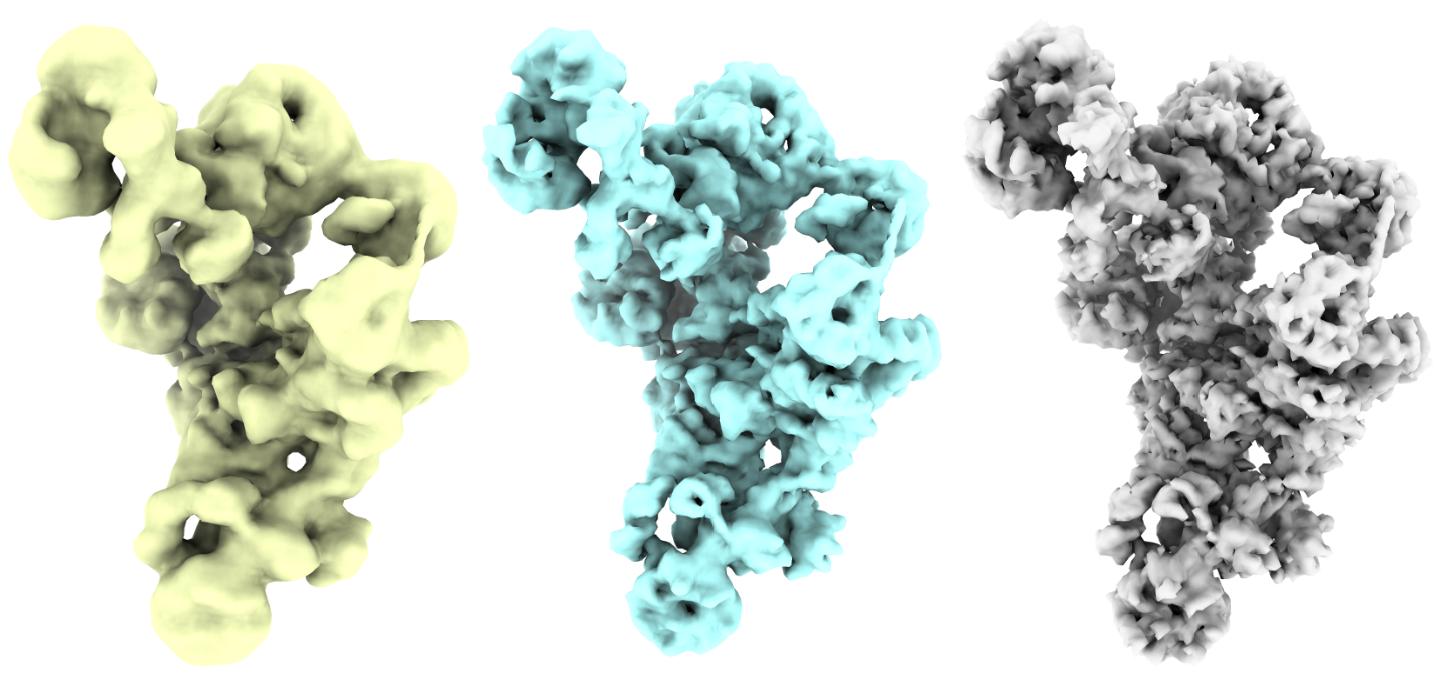
Figure 6: Visualization of the 3D objects of the spliceosome (-10dB). From left to right: reconstructions from cryoAI, ACE-EM with $\mathrm{FourierNet}$ and the ground-truth.

The result of the simulated datasets can be seen in Table 1. Results for CryoPoseNet were taken from previously reported data  [7], cryoDRGN2’s results were from  [20], while the cryoSPARC and cryoAI’s results were obtained by re-running these methods. We found that cryoAI failed frequently due to the spurious structural symmetries even with symmetry loss applied, while ACE-EM rarely failed in reconstructions. The pose estimation accuracy and 3D reconstruction quality are comparable or better than these baseline methods using either $\mathrm{VoxelGrid_{R}}$ or $\mathrm{FourierNet}$ decoder. In terms of reconstruction resolution, ACE-EM with $\mathrm{FourierNet}$ outperformed all the baseline methods. It reached 2 pixels, the Nyquist resolution, using an FSC threshold of 0.5 in all datasets with SNR 200 dB and -10 dB. Visualization of 3D reconstruction results can be found in Figure 5 and Figure 6. Our reconstructed volumes have more details compared to the result of cryoAI. Based on the Nyquist–Shannon sampling theorem  [30], the highest measurable resolution of the dispersed volume representation is 2 pixels. The resolution of ACE-EM with $\mathrm{FourierNet}$ reached the theoretical upper limit, which is not reachable by other methods. To be specific, the FSC correlation coefficient at spatial resolution 2.00 pixels is still very high (0.86) for the spliceosome (200 dB) dataset, well above the standard threshold (0.5). We also benchmarked ACE-EM on an even more challenging dataset (SNR -20 dB; without image shifts). The FSC resolution of the output 3D object reached 2.1 pixels, which is even higher than the results of -10 dB provided by other ML-based baselines. Also, the performance of -20 dB SNR proves the potential of ACE-EM with $\mathrm{FourierNet}$ for working in really low SNR situations.

When using $\mathrm{VoxelGrid_{R}}$ as the decoder, ACE-EM reached a similar or better FSC resolution among other baselines. In detail, on the similar SNR -10dB with the experimental environment, it provided higher resolutions on the spliceosome dataset compared to other baselines (except ACE-EM with $\mathrm{FourierNet}$). With $\mathrm{VoxelGrid_{R}}$, CryoPoseNet failed in the spike datasets, indicating that our method recovered $\mathrm{VoxelGrid_{R}}$’s competitiveness for cryo-EM 3D reconstructions.

For rotation errors and translation errors, our methods get comparable or better results with other baselines. ACE-EM generated fairly accurate pose estimations on noise-free datasets as most baselines. Moreover, ACE-EM performed better on noisy datasets compared to other ML-based methods, especially in terms of the mean rotation error metric.

4.3 3D reconstruction on experimental datasets

Dataset

80S EMPIAR-10028 is an experimental cryo-EM reconstruction dataset used for comparing baselines. The size is downsampled to 128 for cryoDRGN2 and our methods, and it is downsampled to 256 for cryoSPARC and cryoAI due to the failure of reconstruction with cryoAI  [7] in size 128.

Baselines

For experimental datasets, evaluation criterion is half-map FSC  [6] resolution at 0.143, which splits the dataset evenly into two half datasets, then trains the two datasets separately to get two volumes for comparison.

Table 1: Accuracy of pose estimation and 3D reconstruction using per-image pose search (cryoSPARC and cryoDRGN2) and amortized inference (cryoPoseNet, cryoAI, and ACE-EM). Resolution(Res.; unit: pixels), rotation matrix error (Rot.) and translation vector error(Trans.) are listed. ACE-EM with $\mathrm{VoxelGrid_{R}}$ is shown as “ours (V)” and ACE-EM with $\mathrm{FourierNet}$ decoder as “ours (F)”. The best results are in bold and the second-best results are underlined.

		traditional	ML-based
Dataset		cryoSPARC	cryoDRGN2	cryoPoseNet	cryoAI	ours (V)	ours (F)
		per-image pose search		amortized inference
spliceosome	Res.	2.06	-	2.78	2.16	2.23	2.00
$\infty$/200dB	Mean Rot.	0.01	-	-	0.0007	0.004	0.0004
	Med Rot.	0.0003	-	0.004	0.0005	0.0007	0.0003
	Trans.	1.2	-	-	0.9	10.3	1.7
spliceosome	Res.	2.06	-	3.15	2.65	2.00	2.00
-10dB	Mean Rot.	0.01	-	-	0.03	0.005	0.003
	Med Rot.	0.00006	-	0.01	0.003	0.002	0.001
	Trans.	1.2	-	-	3.2	1.7	2.1
spliceosome	Res.	2.24	-	-	-	-	2.10
-20dB	Mean Rot.	0.6	-	-	-	-	1.3
	Med Rot.	0.0007	-	-	-	-	0.02
	Trans.	11.8	-	-	-	-	-
spike	Res.	2.06	-	16.0	2.12	2.85	2.00
$\infty$/200dB	Mean Rot.	0.007	0.0004	-	0.0006	0.05	0.0003
	Med Rot.	0.0007	0.0001	5	0.0004	0.002	0.0002
	Trans.	0.03	-	-	0.7	0.7	1.2
spike	Res.	2.06	2.03	16.0	2.28	2.91	2.00
-10dB	Mean Rot.	0.0005	0.06	-	0.06	0.006	0.003
	Med Rot.	0.0002	0.01	6	0.001	0.002	0.0006
	Trans.	0.03	-	-	0.8	0.4	1.3

Results

The result of the experimental datasets can be see in Table 2. Results for cryoSPARC, cryoDRGN2 and cryoAI were taken from previously reported data  [7], The input image size and output volume size setting for different methods can also be seen in Table 2. CryoAI claimed it is the first amortized inference method to demonstrate proper volume reconstruction on an experimental dataset. However, CryoAI did not properly converge when fed with input images of size 128. A compromise is reached by training with input images with a 256-pixel side but producing a 128-pixel side volume in cryoAI. CryoAI is a standard auto-encoder architecture with $\mathrm{FourierNet}$ as its decoder. Therefore, using ACE-EM with $\mathrm{FourierNet}$ is almost like adding the PIP task to the CryoAI structure. The convergence problem is preliminarily resolved by applying our method. After adding the PIP task, the model can adequately converge with input size ${128\times 128}$. Also, the resolution of ACE-EM with $\mathrm{FourierNet}$ on a 128-pixel input size is better than CryoAI on a 256-pixel input size, which shows the robustness and effectiveness of our method. Meanwhile, the result of ACE-EM with $\mathrm{VoxelGrid_{R}}$ is on the Nyquist resolution, representing its capacity for the experimental situation. Visualization of 3D reconstruction result can be seen in Figure 5.

Table 2: Accuracy of 3D objection reconstruction for experimental 80S ribosome dataset. Resolutions (Res.) are shown in angstroms (Nyquist resolution: 7.54 Å). ACE-EM with $\mathrm{VoxelGrid_{R}}$ and $\mathrm{FourierNet}$ are labeled “ours (V)” and “ours (F)”, respectively.

	traditional	ML-based
80S ribosome (exp.)	cryoSPARC	cryoDRGN2	cryoAI	cryoAI	ours (V)	ours (F)
	per-image pose search		amortized inference
Input image side size	256	128	128	256	128	128
Output volume side size	256	128	128	128	128	128
Final volume side size	128	128	128	128	128	128
Res. Å($\downarrow$)	7.54	7.54	Fail	7.91	7.54	7.66

4.4 Ablation studies

Without PIP, ACE-EM is degenerate into a traditional autoencoder structure. Comparisons are made between training with and without PIP tasks in two different decoders, to prove that our work ACE-EM can boost the performance of an autoencoder by applying PIP regardless of decoder types.

4.4.1 PIP ablation with $\mathrm{FourierNet}$

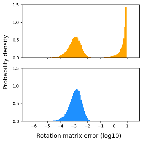
Figure 8: Distribution of rotation matrix prediction errors for the spliceosome dataset (-10 dB). Top: without PIP; Bottom: with PIP.

To test the effect of PIP with $\mathrm{FourierNet}$, we ran an ablation study on the spliceosome dataset (-10 dB) using a batch size of 384 for 300 epochs. As shown in Figure 2, all the performances, including FSC-resolution, mean and median rotation matrix prediction errors, are much worse without the PIP task. Though the median rotation error is similar at the end, the gap in the mean rotation error is noticeable. Without PIP task, the mean rotation error is 1.98 at the 300th epoch, which is three orders of magnitude larger than 0.003, the mean error of ACE-EM. PIP reduces the existence of exaggerated rotation errors(see in Figure 8), then gets a better mean rotation error and further improves the resolution.

We also compare the coverage of the projection orientation space during training in terms of the distribution of the oriented z-axis (projection direction), which is equivalent to the last column of the predicted rotation matrix. When creating the simulated datasets, the projection orientations were sampled from a uniform distribution. Therefore the directions of the oriented z-axis should also be uniformly distributed. As shown in Figure 4, the predicted projection direction vectors covered the entire orientation space with the PIP task starting from epoch 50. In contrast, without the PIP task, the coverage of the orientation space is still incomplete at around 20% in 300 epochs. And the insufficient coverage performance reflected in the large gap between the mean and median rotation errors. After adding PIP task, the training time is increased to 1.25-1.50 times of the original duration for one epoch. But the time consumption is worthy of faster convergence and better performances.

4.4.2 PIP ablation with $\mathrm{VoxelGrid_{R}}$

We also perform an ablation study for the PIP task using $\mathrm{VoxelGrid_{R}}$ as the decoder on the same spliceosome dataset (-10 dB) using a batch size of 1,024 for 300 epochs. As shown in Table 4 and Figure 4, 3D reconstruction failed without either the PIP task or warm-up labeling (Section 3.3). The reconstruction can be completed when using warm-up labeling for loss calculations at the beginning of training. When PIP task was included, the mean rotation matrix prediction error was reduced significantly, and the FSC resolution was also improved.

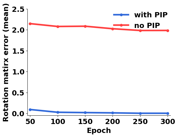
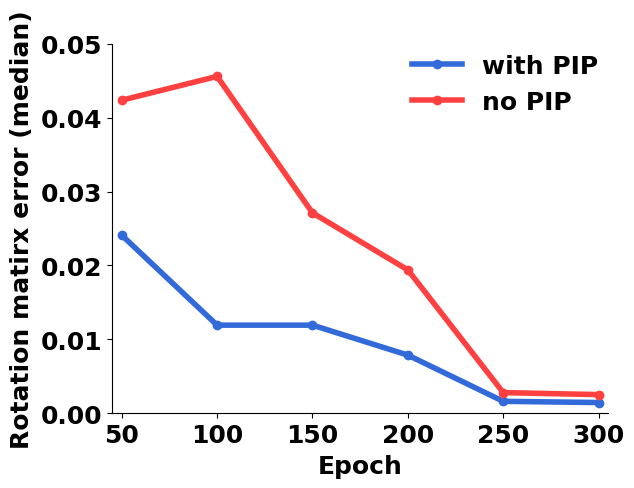
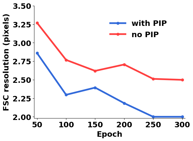
Figure 2: Ablation study with (blue) or without (red) the PIP task using the spliceosome dataset (-10 dB) with $\mathrm{FourierNet}$ as the decoder. Left: mean rotation matrix prediction error. Middle: median rotation matrix prediction error. Right: convergence of the FSC-resolution.

Figure 3: Visualization of the predicted projection directions for the spliceosome dataset (-10 dB). Left: without PIP (epoch 300); Right: with PIP (epoch 50).

Figure 4: 3D reconstruction of the spliceosome dataset (-10 dB) with $\mathrm{VoxelGrid_{R}}$ without (left) or with (middle) the PIP task. The ground-truth is shown on the right.

5 Conclusion

In this work, we have developed a new unsupervised learning framework ACE and applied it to the ab initio cryo-EM 3D reconstruction problem. Compared to existing methods, the most significant advantage of ACE-EM is its ability to learn the pose space much more effectively and accurately. The ACE-EM method can work with different types of decoders, and boost the FSC-resolution even to Nyquist resolution in some simulated and experimental datasets. In the future work on ACE-EM, we plan to extend the ACE framework to work with heterogeneous cryo-EM 3D reconstruction and novel view synthesis for natural images.

6 Reproducibility Statement

The model structure can be seen in Section 3 and appendix A. The datasets and training setup can be seen in Section 4.1. The simulated dataset generation method and the detailed dataset setting can be seen in the appendix B. The code to reproduce our experiments will be open-sourced upon publication.

Appendix A Encoder and decoder

A.1 Encoder $E_{IP}$

The $E_{IP}$ represents a function that maps an input image $Y_{i}$ to its corresponding projection pose parameters $(R_{i},t_{i})$. $R_{i}\in SO(3)\subset\mathbb{R}^{3\times 3}$ is a rotation matrix for mapping a reference orientation to the projection orientation. $t_{i}\in\mathbb{R}^{2}$ is the 2D translation vector to account for the 2D image shift in the input image $Y_{i}$.

$$E_{IP}:Y_{i}\mapsto(R_{i},t_{i})$$ (16)

Cryo-EM projection images are extremely noisy. To improve the $E_{IP}$ performance, we adopted the same image preprocessing strategy as in cryoAI  [7]. Each image $Y_{i}$ is passed on to a set of five Gaussian filters, which are implemented as 2D convolutions with a kernel size of 11 pixels and output a 5-channel image $Y_{i}^{5C}$. The Gaussian kernel variances follow a geometric series, i.e., $10^{-2}$, $10^{-1}$, $1$, $10$, $10^{2}$ in $\text{pixel}^{2}$ for output image channels 1 to 5. The filtered images are given to a ResNet-18  [31] network with two MLP networks for the inference of $R_{i}$ and $t_{i}$ respectively. The raw prediction of $t_{i}$ is passed through a Sigmoid function to restrict the range of values to $(0,1)$, because $t_{i}$ is expressed in unit of fraction of the image edge length. Other feature extractors (FE) can also be used in place of ResNet-18.

$$f_{filter}:Y_{i}\mapsto Y_{i}^{5C}$$ (17)

The complete $E_{IP}$ can be defined as follows, where “$\circ$" means function composition. the trainable parameters are the network work parameters in $f_{FE}$ and $f_{MLP}$.

$$E_{IP}(Y_{i}):=(f_{MLP}\circ f_{FE}\circ f_{filter})(Y_{i})$$ (18)

There are many representations of $R_{i}$ such as Euler angles and quaternions. It has been shown that all 3D rotation representations in the real Euclidean spaces with no more than four dimensions are discontinuous and difficult to learn using neural networks  [32]. We chose the 6-dimensional vector representation in $\mathbb{R}^{3}$  [32], which can be converted into a rotation matrix in $\mathbb{R}^{3\times 3}$ using PyTorch3D  [33].

A.2 Decoder $D_{PI}$

The $D_{PI}$ takes pose $(R_{i},t_{i})$ and predicts the projection image $Y_{i}^{pred}$.

$$D_{PI}:(R_{i},t_{i})\mapsto Y_{i}^{pred}$$ (19)

There are many possible choices for $D_{PI}$. we tested a real-space voxel grid decoder $\mathrm{VoxelGrid_{R}}$ which was used in cryoGAN  [15] and partially used in CryoPoseNet  [22], and a frequency-space neural network decoder $\mathrm{FourierNet}$ from cryoAI  [7]. The trainable parameters of $D_{PI}$ depend on the implementation. In $\mathrm{VoxelGrid_{R}}$, the trainable parameters are stored in a 3D tensor $V\in\mathbb{R}^{L\times L\times L}$, which is a discrete representation of 3D reconstruction target in real space. In $\mathrm{FourierNet}$, the trainable parameters are the network parameters for the two Sinusoidal Representation Networks (SIRENs)  [34] as detailed in cryoAI  [7].

Appendix B Benchmark dataset

To create the ground-truth volumes, we first generate simulated cryo-EM density maps based on published atomic structure coordinate (pdb) files using the molmap command from ChimeraX  [35]. In each density map, each atom is described by a 3D Gaussian distribution with a width proportional to a chosen “resolution" parameter (6 Å  for both proteins). Then, the ground-truth volumes were generated by re-sampling the simulated density maps onto cubic voxel grids with 128 pixels on each side. A set of projection images were generated using cryoSPARC  [14] with uniformly sampled projection orientations over the ground-truth volume. To reduce the difference between the simulated projection images and the experimental ones, random translations and CTF were applied to each projection image. Random translations were sampled from a Gaussian distribution ($\mu=0$, $\sigma=20$ Å).

Table 3:

	Dataset	L	N	Å/pix.	Shift?	SNR(dB)
Simulated	Spike	128	50,000	3.00	N	$\infty$
	Spike	128	50,000	3.00	N	-10
	Spliceosome	128	50,000	4.25	Y	$\infty$
	Spliceosome	128	50,000	4.25	Y	-10
	Spliceosome	128	50,000	4.25	N	-20
Experimental	80S EMPIAR-10028 (downsampled)	128	105,247	3.77	Y	NA

Appendix C Background

Cryo-EM is concerned with the inverse problem of inferring the 3D object associated with a set of projection images $\{Y_{i}\}_{i\in\mathcal{D}}$ where $\mathcal{D}$ is index set for the image dataset. Here we briefly introduce the image formation model in cryo-EM and relevant terminologies.

C.1 Cryo-EM image formation model

Cryo-EM projection images are formed by collecting the electrons scattered by the atoms from macromolecules (e.g., protein molecules) in the sample embedded in thin ice. The raw cryo-EM data are usually referred to as micrographs, which consist of the 2D projections of hundreds of 3D objects. In a so-called “particle picking” step, the projection images of individual 3D objects are cropped out of each micrograph and collected into a stack of projection images.

The 3D reconstruction target object can be defined as a function $V$ for mapping a 3D coordinate to a real value.

$$V:\mathbb{R}^{3}\mapsto\mathbb{R}$$ (20)

Each projection image is associated with a 3D object oriented in a certain direction. Here we focus on the homogenous 3D reconstruction problem where the 3D objects corresponding to all the projection images are identical except for their orientations which can be modeled as a rotation matrix $R_{i}\in SO(3)\subset\mathbb{R}^{3\times 3}$. Each 3D objection can be defined as follows, where the 3D coordinate $\vec{r}=[x,y,z]^{T}$.

$$V_{i}:=V(R_{i}\vec{r})$$ (21)

The projection image $X_{i}$ of object $V_{i}$ is described as integration along the projection direction, usually along the z-axis.

$$X_{i}(x,y):=\int_{\infty}^{\infty}V(R_{i}\vec{r})dz$$ (22)

Due to the wavelike nature of electrons and the magnetic lens systems in the electron microscopes, the projection image signals $X_{i}$ are corrupted by optical interference effects which are modeled by the Point Spread Function (PSF) $f_{PSF}$ in real space or the Contrast Transfer Function (CTF) in Fourier space (see the next section for details). Furthermore, the cropping process of projection images for individual 3D objects from large micrographs is imperfect which can result in small translational image shifts. Lastly, cryo-EM images are affected by noise from various sources  [36] which is assumed to be zero mean, uncorrelated, independently distributed  [37]. A common practice is to model it as a Gaussian noise $\epsilon_{i}\sim\mathcal{N}(0,\sigma^{2}I)$. Taken together, the entire cryo-EM image formation model can be described by the following equation  [7, 38] where $Y_{i}$ is the final projection image considering all factors discussed above, 2D coordinate $\vec{p}=[x,y]^{T}$, and 2D translation $\vec{\tau}=[\Delta x,\Delta y]^{T}$.

$$Y_{i}(\vec{p})=(f_{PSF}\ast X_{i})(\vec{p}+\vec{\tau})+\epsilon_{i}(\vec{p})$$ (23)

Since translation of a function by $\tau$ is equivalent to convolution with a shifted delta function:

$$f(x+\tau)=(\delta_{\tau}\ast f)(x)\text{, where }\delta_{\tau}:=\delta(x+\tau)$$

We can rewrite the above equation as below.

$$Y_{i}(\vec{p})=(\delta_{\vec{\tau}}\ast f_{PSF}\ast X_{i})(\vec{p})+\epsilon_{i}(\vec{p})$$ (24)

The real-space VoxelGrid decoder used in this work was designed based on this image formation model.

C.2 Fourier slice theorem

An alternative and more computationally efficient method of calculating image projection is based on the Fourier slice theorem. It states that the Fourier transformation of a projection image is the same as a slice of the Fourier transform of the corresponding 3D object. The orientation of this slice is the same as the projection plane.

$$\hat{Y}_{i}=\mathcal{S}_{i}[\hat{V}_{i}]$$ (25)

Here $\hat{Y}_{i}$ and $\hat{V}_{i}$ are the Fourier transform of the projection image $Y_{i}$ and $\hat{V}_{i}$, respectively. $S_{i}$ is the volume slicing operator which is defined as a mapping from frequency coordinates $\vec{k}=[k_{x},k_{y},k_{z}]^{T}$ on a rotated 2D Fourier plane (passing through the origin) to the value of $\hat{V}_{i}$ at that point in Fourier space.

$$\hat{S}_{i}[\hat{V}_{i}](k_{x},k_{y}):=\hat{V}(R_{i}\vec{k})|_{k_{z}=0}$$ (26)

Using the Fourier slice theorem, the cryo-EM image formation model in Fourier space can be simplified as follows, where 2D frequency coordinate $\vec{q}=[k_{x},k_{y}]^{T}$.

$$\hat{Y}_{i}(\vec{q}):=F_{\vec{\tau}}(\vec{q})\cdot F_{\text{CTF}}(\vec{q})\cdot S_{i}[\hat{V}](\vec{q})+\hat{\epsilon}(\vec{q})$$ (27)

$F_{\text{CTF}}$ is the contrast transfer function which is the Fourier transform of the Point Spread Function  [37]. $\hat{\epsilon}$ is the Gaussian white noise in Fourier space. $F_{\vec{\tau}}$ is the phase-shift function defined below, which is equivalent to translation by $\vec{\tau}$ in real space: $F_{\vec{\tau}}(\vec{q}):=e^{-2\pi i\vec{\tau}\cdot\vec{q}}$. A majority of the cryo-EM 3D reconstruction algorithms are based on this theorem, such as RELION  [13], cryoSPARC  [14], cryoDRGN  [18, 19, 20], and cryoAI  [7].

Appendix D Visualization of 2D images and 3D reconstruction

Visulization of the 2D projection images involved in the ACE-EM method is shown in  5. An example of the 3D reconstruction results is shown in  6.

Figure 5: Visualization of the predicted 3D objects (in blue color) and the ground-truth (in gray color) at two different viewing angles. Left: reconstruction of the spike (200 dB) dataset using $\mathrm{FourierNet}$. Right: reconstruction of 80S ribosome using $\mathrm{VoxelGrid_{R}}$ with half of the experimental dataset. The approximate ground-truth volume for 80S ribosome was constructed by cryoSPARC using the entire set of experimental projection images (L = 360 pixels) and then downsampled to a smaller size (L = 128 pixels).

Figure 7: Visualization of the input and predicted 2D projection images by ACE-EM on the spliceosome datasets at different noise levels. From left to right: The original images from the input datasets, the intermediate projection images generated by the decoder ($\mathrm{FourierNet}$), the final predicted images with CTF and noise applied. From top to bottom: datasets with SNR at 200 dB, -10 db, and -20 dB, respectively.

Appendix E Ablation study of the PIP task

Ablation study results for the PIP task are shown in  4,  2, and  8.

Table 4: Ablation study for the PIP task with $\mathrm{VoxelGrid_{R}}$. “Warm-up labeling” refers to using Gaussian-filtered input images as labels for loss calculation . FSC resolution (Res.) was calculated at a threshold of 0.5 against ground-truth volume (unit: pixels). Rotation errors (Rot.) are measured by mean and median values.

PIP task	Warm-up labeling	Res.	Rot. (mean)	Rot. (median)
No	No	N/A	N/A	N/A
No	Yes	2.24	1.124	0.005
Yes	Yes	2.20	0.008	0.004

References

- [1] Joachim Frank. Advances in the field of single-particle cryo-electron microscopy over the last decade. Nature Protocols, 12:209–212, 2017.
- [2] Tristan Bepler, Kotaro Kelley, Alex J. Noble, and Bonnie Berger. Topaz-Denoise: general deep denoising models for cryoEM and cryoET. Nature Commun., 11:5208, 2020.
- [3] C. Donnat, A. Levy, F. Poitevin, and N. Miolane. Deep generative modeling for volume reconstruction in cryo-electron microscopy. arXiv, 2201.02867, 2022.
- [4] Ian Goodfellow, Jean Pouget-Abadie, Mehdi Mirza, Bing Xu, David Warde-Farley, Sherjil Ozair, Aaron Courville, and Yoshua Bengio. Generative adversarial nets. In Advances in neural information processing systems, pages 2672–2680, 2014.
- [5] Mark A. Kramer. Nonlinear principal component analysis using autoassociative neural networks. AIChE Journal, 37:233–243, 1991.
- [6] Peter B Rosenthal and John L Rubinstein. Validating maps from single particle electron cryomicroscopy. Current Opinion in Structural Biology, 34:135–144, 2015.
- [7] A. Levy, F. Poitevin, J. Martel, Y. Nashed, A. Peck, N. Miolane, D. Ratner, M. Dunne, and G. Wetzstein. CryoAI: Amortized Inference of Poses for ab initio Reconstruction of 3D Molecular Volumes from Real Cryo-EM Images. In European Conference on Computer Vision (ECCV), 2022.
- [8] Ben Mildenhall, Pratul P. Srinivasan, Matthew Tancik, Jonathan T. Barron, Ravi Ramamoorthi, and Ren Ng. NeRF: Representing scenes as neural radiance fields for view synthesis. volume 65, pages 99–106, 2021.
- [9] Alex Yu, Sara Fridovich-Keil, Matthew Tancik, Qinhong Chen, Benjamin Recht, and Angjoo Kanazawa. Plenoxels: Radiance fields without neural networks. In 2022 IEEE/CVF Conference on Computer Vision and Pattern Recognition (CVPR), pages 5491–5500, 2022.
- [10] Cheng Sun, Min Sun, and Hwann-Tzong Chen. Improved direct voxel grid optimization for radiance fields reconstruction, 2022.
- [11] Chen-Hsuan Lin, Wei-Chiu Ma, Antonio Torralba, and Simon Lucey. BARF: Bundle-adjusting neural radiance fields. In 2021 IEEE/CVF International Conference on Computer Vision (ICCV), pages 5721–5731, 2021.
- [12] Yoonwoo Jeong, Seokjun Ahn, Christopher B. Choy, Animashree Anandkumar, Minsu Cho, and Jaesik Park. Self-calibrating neural radiance fields. In Proceedings of the IEEE/CVF International Conference on Computer Vision (ICCV), pages 5846–5854, 2021.
- [13] Sjors H.W. Scheres. Relion: Implementation of a bayesian approach to cryo-em structure determination. Journal of Structural Biology, 180:519–530, 2012.
- [14] Ali Punjani, John L. Rubinstein, David J. Fleet, and Marcus A. Brubaker. cryoSPARC: algorithms for rapid unsupervised cryo-EM structure determination. Nature Methods, 14:290–296, 2017.
- [15] Harshit Gupta, Michael T. McCann, Laurène Donati, and Michael Unser. Cryogan: A new reconstruction paradigm for single-particle cryo-em via deep adversarial learning. IEEE Transactions on Computational Imaging, 7:759–774, 2021.
- [16] Harshit Gupta, Thong H. Phan, Jaejun Yoo, and Michael Unser. Multi-CryoGAN: Reconstruction of Continuous Conformations in Cryo-EM Using Generative Adversarial Networks. In Computer Vision – ECCV 2020 Workshops, pages 429–444, 2020.
- [17] Karen Ullrich, Rianne van den Berg, Marcus A. Brubaker, David J. Fleet, and Max Welling. Differentiable probabilistic models of scientific imaging with the Fourier slice theorem. In Proceedings of The 35th Uncertainty in Artificial Intelligence Conference, PMLR, 2020.
- [18] Ellen D. Zhong, Tristan Bepler, Joseph H. Davis, and Bonnie Berger. Reconstructing continuous distributions of 3d protein structure from cryo-em images. In International Conference on Learning Representations, 2019.
- [19] Ellen D. Zhong, Tristan Bepler, Bonnie Berger, and Joseph H. Davis. Cryodrgn: reconstruction of heterogeneous cryo-em structures using neural networks. Nature Methods, 18:176–185, 2021.
- [20] Ellen D. Zhong, Adam Lerer, Joseph H. Davis, and Bonnie Berger. CryoDRGN2: ab initio neural reconstruction of 3D protein structures from real cryo-em images. In 2021 IEEE/CVF International Conference on Computer Vision (ICCV), pages 4046–4055, 2021.
- [21] Dan Rosenbaum, Marta Garnelo, Michal Zielinski, Charlie Beattie, Ellen Clancy, Andrea Huber, Pushmeet Kohli, Andrew W. Senior, John Jumper, Carl Doersch, S. M. Ali Eslami, Olaf Ronneberger, and Jonas Adler. Inferring a continuous distribution of atom coordinates from cryo-em images using VAEs, 2021.
- [22] Youssef S. G. Nashed, Frédéric Poitevin, Harshit Gupta, Geoffrey Woollard, Michael Kagan, Chun Hong Yoon, and Daniel Ratner. Cryoposenet: End-to-end simultaneous learning of single-particle orientation and 3d map reconstruction from cryo-electron microscopy data. In Proceedings of the IEEE/CVF International Conference on Computer Vision (ICCV) Workshops, pages 4066–4076, October 2021.
- [23] Diederik P Kingma and Max Welling. Auto-encoding variational bayes. In International Conference on Learning Representations, 2014.
- [24] Ali Punjani and David J. Fleet. 3D Flexible Refinement: Structure and Motion of Flexible Proteins from Cryo-EM, 2021. bioRxiv:2021.04.22.440893.
- [25] Xun Huang, Ming-Yu Liu, Serge Belongie, and Jan Kautz. Multimodal unsupervised image-to-image translation. In Proceedings of the European Conference on Computer Vision (ECCV), September 2018.
- [26] Hsin-Ying Lee, Hung-Yu Tseng, Qi Mao, Jia-Bin Huang, Yu-Ding Lu, Maneesh Singh, and Ming-Hsuan Yang. DRIT++: Diverse image-to-image translation via disentangled representations. Int. J. Comput. Vision, 128:2402–2417, 2020.
- [27] Abel Gonzalez-Garcia, Joost van de Weijer, and Yoshua Bengio. Image-to-image translation for cross-domain disentanglement. In Advances in Neural Information Processing Systems, volume 31, 2018.
- [28] A. Konstantinidis. 2.02 - physical parameters of image quality. In Anders Brahme, editor, Comprehensive Biomedical Physics, pages 49–63. Elsevier, Oxford, 2014.
- [29] Ilya Loshchilov and Frank Hutter. Fixing weight decay regularization in adam. arXiv, 1711.05101, 2017.
- [30] C.E. Shannon. Communication in the presence of noise. Proceedings of the IRE, 37(1):10–21, 1949.
- [31] Kaiming He, Xiangyu Zhang, Shaoqing Ren, and Jian Sun. Deep residual learning for image recognition. In Proceedings of the IEEE conference on computer vision and pattern recognition, pages 770–778, 2016.
- [32] Yi Zhou, Connelly Barnes, Jingwan Lu, Jimei Yang, and Hao Li. On the continuity of rotation representations in neural networks. In 2019 IEEE/CVF Conference on Computer Vision and Pattern Recognition (CVPR), pages 5738–5746, 2019.
- [33] Justin Johnson, Nikhila Ravi, Jeremy Reizenstein, David Novotny, Shubham Tulsiani, Christoph Lassner, and Steve Branson. Accelerating 3d deep learning with pytorch3d. In SIGGRAPH Asia 2020 Courses, New York, NY, USA, 2020. Association for Computing Machinery.
- [34] Vincent Sitzmann, Julien Martel, Alexander Bergman, David Lindell, and Gordon Wetzstein. Implicit neural representations with periodic activation functions. Advances in Neural Information Processing Systems, 33:7462–7473, 2020.
- [35] Eric F. Pettersen, Thomas D. Goddard, Conrad C. Huang, Elaine C. Meng, Gregory S. Couch, Tristan I. Croll, John H. Morris, and Thomas E. Ferrin. UCSF ChimeraX: Structure visualization for researchers, educators, and developers. Protein Science, 30:70–82, 2021.
- [36] William T. Baxter, Robert A. Grassucci, Haixiao Gao, and Joachim Frank. Determination of signal-to-noise ratios and spectral SNRs in cryo-EM low-dose imaging of molecules. Journal of Structural Biology, 166:126–132, 2009.
- [37] Pawel A. Penczek. Single-particle cryo-electron microscopy: Mathematical theory, computational challenges, and opportunities. Methods in Enzymology, 482:35–72, 2010.
- [38] Tamir Bendory, Alberto Bartesaghi, and Amit Singer. Single-particle cryo-electron microscopy: Mathematical theory, computational challenges, and opportunities. IEEE Signal Processing Magazine, 37(2):58–76, 2020.