Two-dimensional electron gas under the effect of constrained potential and magnetic field in curved space

Abstract

The effect of the curvature of a cylindrical surface on the energy spectrum for a curved two dimensional electron gas in a homogeneous magnetic field is considered.The corrections to the energy spectrumis obtained for the first time perturbatively, in contrast to previous works where it was obtained numerically. The dispersion relationship is obtained as a function of curvature radius and the results for curved surface have been compared with the flat surface.

Keywords: Two-dimensional electron gas, Curvature radius, Constrained potential, Geometric potential

PACS numbers: 73,43,Fj, 73,23,Ad, 73,43,Qt

1 Introduction

In quantum mechanics, one of the ways that can be discussed about the motion of a particle rigidly bounded on a surface is confining potential approach, in that the particle is confined by a strong force that acts normally to our surface in all points of the space.This idea can be readily put in practice considering a potential which is constant over the surface but increases sharply for every small displacement in the normal direction to the surface. The confining potential approach yields a unique effective Hamiltonian that depends on physical mechanism of the constraint [1, 2, 3]. The Hamiltonian contains the surface potential as the quantum potential that is dependent on mean and Gaussian curvatures[1, 4, 5]. One of the greatest achievements in solid state physics is the fabrication of low dimensional systems. An example of a low dimensional system is the two-dimensional electron gas (2DEG). The electrical behavior of a (2DEG) subjected to a uniform magnetic field has been studied in much detail [6, 7, 8]. In the ballistic regime, the system is characterized by stationary Landau states. A proemial label of two dimensional implied that these electron systems were flat. The physics of nanostructures and quantum waveguide may pose questions concerning curved surface in quantum theory, which is increasingly relevant to device modelling [9, 10]. Two-dimensional electron gas (2DEG) in the planar heterostructures has been investigated greatly, which lead to in finding a number of remarkable quantum phenomena such as, integer and fractional quantum Hall effects, the Berry quantum phase,etc. Non-planar low-dimensional structures are fundamentally new physical objects that have attracted the attention of the researchers during last recent years[8, 11, 12, 13, 14, 10, 15, 16, 17, 18, 19, 20].
Experimentally non-planar surfaces with 2DEG were synthesized by means of molecular-beam epitaxy on faceted surfaces [21, 22] and were typically realized at nearly atomically smooth interfaces of single-crystalline semiconductors [23]. The main drawback of such structures is spatial fluctuations of the curvature of surface in them, which makes the studies of the effect of the curvature on the magnetotransport [24] in such structures a very difficult task. The cylindrical surface is the simplest model for investigating the influence of geometry on physical systems[25, 26]. The interest in the electronic properties of quantum systems with cylindrical symmetry has received a boost, because the early proposals of carbon nanotubes[27, 28] for building future nanoelectronic devices, have interesting mechanical and electrical properties. In this paper, curved two-dimensional electron gas with cylindrical symmetry was considered in a homogeneous magnetic field. The energy spectrum of the electrons on a cylinder surface have been obtained by studying the geometry potential as the constraint.

2 Hamiltonian of a 2DEG in a magnetic field

Let us consider a spinless electron in two dimensions constrained to move along a surface $s$ of curve $C$ (curved two-dimensional electron gas (C2DEG)) by the action of external forces. For this purpose, we consider a curved two-dimensional electron gas (2DEG) in a uniform magnetic field $\vec{B}=B\cos(\varphi)\hat{z}$ that is shown in Fig.1. Without any restriction on the problem and just for simplicity, we assume that the equation of the surface is $z=f(x)$, where $f(x)$ is an arbitrary function which depend on the variable $y$. According to Fig.1, the arc length of $C$ (the distance parameter on the surface).i.e $s$ is defined by

$$s(x)=\int_{0}^{x}\sqrt{{1+f^{{}^{\prime}}}^{2}(x)}dx{\color[rgb]{1,0,0},}$$ (1)

where the coordinate $x(s)$ is function of the arc length of $C$. The problem then reduces to solving the Schrodinger equation

$$\frac{1}{2m}\Big{[}({\mathbf{P}}-\frac{e}{c}{\mathbf{A}})^{2}+V_{\lambda}(z)\Big{]}\psi(s,y,z)=E\psi(s,y,z){\color[rgb]{1,0,0}.}$$ (2)

Since in quantum mechanics, we can no longer predict the position of the particle with point like accuracy, it is natural to consider only constraint forces that are orthogonal to the curve $C$ in all points of the plane, where the particle can possibly be found. In order to satisfy this requirement, we shall consider potentials which have constant values over $C$ but are increased sharply for every small displacement along normals of $C$. It can be easily see that this result may be obtained by choosing potentials $V_{\lambda}(z)$ (independent of $s$). For this purpose the constraining process can be defined as being produced by a family of increasingly stranger potentials $V_{\lambda}(z)$, where $\lambda(z)$ is a squeezing parameter which defines the strength of the potential [1]

$$V_{\lambda}(z)=\left\{\begin{array}[]{cc}0&z=0\\ \infty&z\neq 0\end{array}\right\}{\color[rgb]{1,0,0}.}$$ (3)

Taking the magnetic field $\vec{B}=(0,0,B\cos\phi)$ according to the Fig.1, the vector potential is $\vec{A}=(0,Bx(s),0)$.
Eq.(2) can now be easily separated by setting $\psi(s,y,z)=Y(s,y).Z(z)$ where $Y(s,y)$ is the tangential component of the wave function

$$\frac{-\hbar^{2}}{2m}\frac{\partial^{2}Z(z)}{\partial{z}^{2}}+V_{\lambda}(z)Z(z)=i\hbar\frac{\partial Z(z)}{\partial{t}}{\color[rgb]{1,0,0},}$$ (4)

$$\frac{-\hbar^{2}}{2m}\frac{\partial^{2}{Y(s,y)}}{\partial{s}^{2}}+\frac{-\hbar^{2}}{2m}\frac{\partial^{2}{Y(s,y)}}{\partial{y}^{2}}+\frac{1}{2}m\omega_{c}^{2}x^{2}(s)Y(y,s)+i\hbar\omega_{c}x(s)$$

$$\frac{\partial{Y(y,s)}}{\partial{y}}+U(s,y)Y(y,s)=EY(y,s){\color[rgb]{1,0,0},}$$ (5)

where $\omega_{c}=eB/mc$.
Eq.(4) that is just a one-dimensional Schrodinger equation for a particle bounded by the transverse potential $V_{\lambda}(z)$, can be ignored in all future calculation. Eq. (5) is much more interesting, due to the presence of the surface potential $U(s,y)$. In the case of a 2DEG flexing the gas leads to a geometric potential of the form [1]

$$U=\frac{-\hbar^{2}}{8m}[\kappa_{1}(s)-\kappa_{2}(s)]^{2}=\frac{-\hbar^{2}}{8m}\Big{(}\frac{1}{R_{1}(s)}-\frac{1}{R_{2}(s)}\Big{)}^{2}{\color[rgb]{1,0,0},}$$ (6)

where $m$ is the effective mass and $R_{1}$,$R_{2}$ are the principal curvature radii of the surface at the point where the electron resides[2, 3].
The surface potential (geometric potential) is always attractive and is independent of the electric charge of particle, similar to gravitation.
Furthermore, it is of purely quantum origin, i.e. it vanishes for the limit $\hbar\longrightarrow 0$.
If one of the radii tends to infinity, we obtain a cylindrical surface, particularly, one confined to a quantum wire having the shape of a plane curve as (seen in Fig.1). The geometric potential (surface potential $C$), for such system reads as[1]

$$U(s)=-\frac{\hbar^{2}}{8mR^{2}(s)}{\color[rgb]{1,0,0}.}$$ (7)

The Hamiltonian of Eq.(5) dose not contain $y$ and the $p_{y}$ is a constant of motion with the value of $\hbar k$. The wave function $Y(s,y)$ in $y$ direction as planar waves $e^{iky}$ and in $s$ direction is as function of $s$, therefore, we can assume

$$Y(s,y)=e^{iky}p(s){\color[rgb]{1,0,0}.}$$ (8)

Substituting Eq.(8) in Eq.(5) we can obtain the Hamiltonian of electron gas in two dimensional as [25]

$$H=\frac{-\hbar^{2}}{2m}\frac{\partial^{2}}{\partial{s}^{2}}+\frac{1}{2}m\omega_{c}^{2}\Big{(}x(s)-\frac{\hbar k}{m\omega_{c}}\Big{)}^{2}-\frac{\hbar^{2}}{8mR^{2}(s)}{\color[rgb]{1,0,0}.}$$ (9)

Note that for $f^{\prime}(x)\ll 1$, we can expand Eq.(1) and by using one order approximation, we have

$$s(x)\approx x(s).$$

Let us define the coordinates $x^{\prime}(s)$ and $s^{\prime}(x)$ as

$$x^{\prime}(s)=x(s)+\frac{\hbar k}{m\omega_{c}}{\color[rgb]{1,0,0},}\;\;\;\;\;s^{\prime}(x)=s(x)+\frac{\hbar k}{m\omega_{c}}{\color[rgb]{1,0,0},}$$ (10)

which allow us to rewrite the Eq.(9) in two parts as

$$H=H_{os}+\frac{1}{2}m\omega_{c}^{2}\Big{[}x^{\prime 2}(s)-s^{\prime 2}(x)\Big{]}-\frac{\hbar^{2}}{8mR^{2}(s)}{\color[rgb]{1,0,0},}$$ (11)

where $H_{os}$ is Hamiltonian of a simple harmonic oscillator. Note that since the distance parameter on cylinder surface $s(x)$ of Fig.1 is small, it is convenient to consider second and third terms of Eq.(11), as a perturbation Hamiltonian.

3 The energy spectrum

In this section, the time independent perturbation theory is used and then the energy spectrum is calculated, thus we have,

$${\color[rgb]{1,0,0}H^{\prime}}=\frac{1}{2}m\omega_{c}^{2}\Big{[}x^{\prime 2}(s)-s^{\prime 2}(x)\Big{]}-\frac{\hbar^{2}}{8mR^{2}}{\color[rgb]{1,0,0}.}$$ (12)

The first order energy shift is obtained by

$$E_{n}^{1}=\frac{1}{2}m\omega_{c}^{2}\Big{[}\langle n|x^{\prime 2}(s)|n\rangle-\langle n|s^{\prime 2}(x)|n\rangle\Big{]}-\frac{\hbar^{2}}{8mR^{2}}\langle n|n\rangle{\color[rgb]{1,0,0}.}$$ (13)

In order to calculate the first and second terms of the Eq.(13), let us define in Fig.1

$$x^{\prime}(s)=R\sin(\frac{s(x)}{R})+\frac{\hbar k}{m\omega_{c}}{\color[rgb]{1,0,0}.}$$ (14)

Substituting Eq.(14) into Eq.(13) we can find

$$\langle n|x^{\prime 2}(s)|n\rangle=R^{2}\Big{[}\langle n|(-\frac{1}{4}\exp(\frac{2\imath\hat{s}}{R})+\exp(-\frac{2\imath\hat{s}}{R})-2)|n\rangle\Big{]}$$

$$+\frac{\hbar^{2}k^{2}}{m^{2}\omega^{2}_{c}}+\frac{2\hbar kR}{m\omega_{c}}\Big{[}\langle n|\frac{1}{2\imath}(\exp(\frac{\imath\hat{s}}{R})-\exp(-\frac{\imath\hat{s}}{R}))|n\rangle\Big{]}$$

$$\langle n|s^{\prime 2}(x)|n\rangle=\frac{\hbar}{2m\omega_{c}}(2n+1){\color[rgb]{1,0,0}.}$$ (15)

It is convenient to define two non-Hermitian operators as

$$\hat{a}=\sqrt{\frac{m\omega}{2\hbar}}(\hat{s}+\frac{i\hat{p}}{m\omega}){\color[rgb]{1,0,0},}\;\;\;\;\;\;\;\;\hat{a}^{{\dagger}}=\sqrt{\frac{m\omega}{2\hbar}}(\hat{s}-\frac{i\hat{p}}{m\omega}){\color[rgb]{1,0,0},}$$ (16)

where $p=i\hbar\partial/\partial{s}$.
Using the Eqs. (3) and (16), the Eq.(13) reduce to

$$E_{n}^{1}=\frac{1}{2}m\omega_{c}^{2}\Big{[}\frac{R^{2}}{2}-\frac{R^{2}}{4}[\langle n|e^{\frac{2i}{R}\sqrt{\frac{\hbar}{2m\omega_{c}}}(\hat{a}+\hat{a^{{\dagger}}})}|n\rangle e^{\frac{-2i\hbar k}{m\omega_{c}R}}+\langle n|e^{\frac{-2i}{R}\sqrt{\frac{\hbar}{2m\omega_{c}}}(\hat{a}+\hat{a^{{\dagger}}})}|n\rangle$$

$$e^{\frac{2i\hbar k}{m\omega_{c}R}}]+\frac{\hbar^{2}k^{2}}{m^{2}\omega_{c}^{2}}+\frac{\hbar kR}{im\omega_{c}}[\langle n|e^{\frac{i}{R}\sqrt{\frac{\hbar}{2m\omega_{c}}}(\hat{a}+\hat{a^{{\dagger}}})}|n\rangle e^{\frac{-i\hbar k}{m\omega_{c}R}}-\langle n|e^{\frac{-i}{R}\sqrt{\frac{\hbar}{2m\omega_{c}}}(\hat{a}+\hat{a^{{\dagger}}})}|n\rangle e^{\frac{i\hbar k}{m\omega_{c}R}}]$$

$$-\frac{\hbar}{2m\omega_{c}}(2n+1)\Big{]}-\frac{\hbar^{2}}{8mR^{2}}\langle n|n\rangle{\color[rgb]{1,0,0}.}$$ (17)

Let us define the dimensionless parameters $\alpha$ and $\beta$ as

$$\alpha=\frac{2}{R}\sqrt{\frac{\hbar}{2m\omega_{c}}},\;\;\;\;\;\;\beta=\frac{2\hbar k}{m\omega_{c}R}{\color[rgb]{1,0,0}.}$$ (18)

Using the formula

$$\langle n|(\hat{a^{\dagger}})^{\ell}\hat{a}^{m}|n\rangle=\frac{n!}{(n-l)!}\delta_{\ell,m}{\color[rgb]{1,0,0},}$$

$$e^{\hat{A}+\hat{B}}=e^{\hat{A}}e^{\hat{B}}e^{-\frac{1}{2}[\hat{A},\hat{B}]}{\color[rgb]{1,0,0},}$$

$$e^{x}=\sum_{0}^{\infty}\frac{x^{n}}{n!}{\color[rgb]{1,0,0},}$$ (19)

we find the energy spectrum for the first order of $n$ of a curved (2DEG) under a homogenous field in cylindrical geometry as

$$E_{n}=E_{n}^{0}+E_{n}^{1}=(n+\frac{1}{2})\hbar\omega_{c}+\frac{1}{4}m\omega_{c}^{2}R^{2}\Big{[}1-e^{-\frac{1}{2}\alpha^{2}}\cos(\beta)\sum_{m=0}^{n}\frac{(i\alpha)^{2m}}{(m!)^{2}}\frac{n!}{(n-m)!}$$

$$-\frac{4\hbar k}{m\omega_{c}R}e^{-\frac{1}{4}\alpha^{2}}\sin(\frac{\beta}{2})\sum_{m=0}^{n}\frac{(i\alpha/2)^{2m}}{(m!)^{2}}\frac{n!}{(n-m)!}\Big{]}+\frac{\hbar^{2}k^{2}}{2m}-\frac{1}{4}\hbar\omega_{c}(2n+1)$$

$$-\frac{\hbar^{2}}{8mR^{2}}{\color[rgb]{1,0,0}.}$$ (20)

The dependence of Eq.(3) on curvature radius R for a cylindrical surface is remarkable and has an important consequence. In order to illustrate the dynamical properties of Eq.(3), the energy spectrum as a function of curvature radius R in the Fig.2 has been plotted for the states $n=0,1,2,\ldots$. For small radii R, the drop energy spectrum is observed and for large radii $R$ ($R\longrightarrow\infty$) the energy spectrum is independent of $R$ and the energy levels have an asymptotic behaviour as the radius $R$ increases.
Note that Eq.(3) for $R\longrightarrow\infty$ deduces to

$$E_{n}=(n+\frac{1}{2})\hbar\omega_{c}{\color[rgb]{1,0,0}.}$$ (21)

This equation has a common expression (in landau gauge) for a flat 2DEG in a perpendicular magnetic field [13, 14]. In order to evaluate the results obtained in Eq. (3), we have compared Fig.2 with plot3 and plot5 which were obtained numerically in [26]. These figures show that the energy levels versus the radius $R$ of the cylinder have an asymptotic behaviour as $R$ increases. In the limit $R\rightarrow\infty$, they become the Landau levels for an electron in a flat space[26].
Due to technological progress, the physics of curved two-dimensional quantum system with cylindrical symmetry is important both theoretically and experimentally [29]. Therefore, with study of energy spectrum of these systems, we can investigate the role of curvature in electronics as magnetotransport [24] and quantum electromechanical circuits[9]. Using the Eq. (3), we will study in future works of the magnetic properties of curved two-dimensional electron gas as the chemical potential, ground-state energy and magnetic susceptibility.

4 Curved 2DEGS in high magnetic fields

Curved 2DEGs in magnetic fields without surface potential(geometric potentials)in high magnetic fields are studied in [15]. In this section, we apply this approach and consider influence of curvature (term relevant to the surface potential)directly in the equation of motion (the Schrodinger equation). The energy spectrum will be found for a two dimensional electron gas under the a magnetic field. For this purpose, we assume that two-dimensional electron gas in component plane of the magnetic field does not influence the energetic structure of the system strictly. The geometry of a curved 2DEG in a homogeneous magnetic field is shown in Fig.3.The Schrodinger Eq.(2) for cylinder 2DEG is given by

$$\frac{1}{2m}\Big{[}({\mathbf{P}}-\frac{e}{c}{\mathbf{A}})^{2}-\frac{\hbar^{2}}{8mR^{2}}\Big{]}\psi(x,y)=E\psi(x,y){\color[rgb]{1,0,0}.}$$ (22)

According to the Fig.3, we consider a magnetic field perpendicular to the cylinder as $\vec{B}=(0,0,Bcos\varphi)$, with an intensity $B$, and a convenient choice for the vector potential in asymmetric gauge is $\vec{A}=(0,BRcos\varphi,0)$. Therefore, substituting vector potential in the Eq.(22) and after some mathematical calculations, we find

$$\frac{-\hbar^{2}}{2m}\frac{\partial^{2}{\psi(x)}}{\partial{x}^{2}}+\frac{1}{2}m\omega_{c}^{2}(R\sin\frac{x}{R}-\frac{\hbar k_{y}}{eB})^{2}\psi(x)-\frac{\hbar^{2}}{8mR^{2}}\psi(x)=E\psi(x){\color[rgb]{1,0,0},}$$ (23)

where $\omega_{c}=eB/mc$, is the cyclotron frequency and $k_{y}$ is the wave vector of motion in y-direction. Note that the Eq. (23) for $R\longrightarrow\infty$ reduces to the flat 2DEG in a perpendicular magnetic field as

$$\frac{-\hbar^{2}}{2m}\frac{\partial^{2}{\psi(x)}}{\partial{x}^{2}}+\frac{1}{2}m\omega_{c}^{2}(x-x_{0})^{2}\psi(x)=E\psi(x){\color[rgb]{1,0,0},}$$ (24)

where $x_{0}=\hbar k_{y}/eB$ is the apex of parabola that is created by magnetic field. Eq.(23) can be simplified by presentating local coordinates around the minimum $x_{m}=R\arcsin(x_{0}/R)$ of the term in parenthesis

$$\sin\frac{x_{m}+x^{\prime}}{R}-\frac{x_{0}}{R}=\sin\frac{x_{m}}{R}\underbrace{\cos\frac{x^{\prime}}{R}}_{\approx 1}+\cos\frac{x_{m}}{R}\underbrace{\sin\frac{x^{\prime}}{R}}_{\approx x^{\prime}/R}-\frac{x_{0}}{R}\approx\frac{x^{\prime}}{R}\cos\frac{x_{m}}{R}{\color[rgb]{1,0,0}.}$$ (25)

Here we assume that the local coordinate $x^{\prime}\ll R$. Since the radius of curvature $R$ is of the order $10^{-4}m$ in Fig.4, whereas the local coordinate is relevant on the scale of the magnetic length $(\approx 25\;nm\;at\;1\;T),$ this assumption is well satisfied [6, 15, 16, 17].
Substituting Eq.(25) into the Eq.(23), we have

$$\frac{-\hbar^{2}}{2m}\frac{\partial^{2}{\psi(x)}}{\partial{x^{2}}}+\frac{1}{2}m(\omega_{c}\cos\frac{x_{m}}{R})^{2}(x-x_{m})^{2}\psi(x)-\frac{\hbar^{2}}{8mR^{2}}\psi(x)=E\psi(x){\color[rgb]{1,0,0},}$$ (26)

which is equivalent to Eq.(24) only with difference that the effective magnetic field is $B_{eff}=B\cos(x_{m}/R)$, we find energy spectrum of a curved 2DEG in cylindrical geometry as

$$E_{n}=(n+\frac{1}{2})\hbar\omega_{c}\cos\frac{x_{m}}{R}-\frac{\hbar^{2}}{8mR^{2}}=(n+\frac{1}{2})\hbar\omega_{c}\cos(\arcsin\frac{x_{0}}{R})-\frac{\hbar^{2}}{8mR^{2}}$$

$$E_{n}=(n+\frac{1}{2})\hbar\omega_{c}\sqrt{1-\frac{x_{0}^{2}}{R^{2}}}-\frac{\hbar^{2}}{8mR^{2}}{\color[rgb]{1,0,0}.}$$ (27)

Eq. (27) shows that the landau levels which are dispersionless in the planar case, now have a semielliptical dispersion as a function of $R$ and $B$. The Eq.(27) is valid for the energy spectrum of a single-particle state of a two-dimensional electron gas confined to the surface of a cylinder immersed in a magnetic field. In Fig.4, energy spectrum is shown curvature plots for the states $n=0,1,\ldots$. For small radii $R$, the low energy spectrum is observed and for large radii $R$ ($R\longrightarrow\infty$), it is independent of, $R$ i.e. the flat 2DEG. In order to evaluate the validity of Eq. (3), we are comparing Figs .2and 4. It can be concluded that the dependence to curvature $R$ for Fig. 2 is more. This dependence can also be seen for some values of the dimensionless parameters $\alpha$ and $\beta$ in Eq. (3). The energy spectrums in Eqs. (3) and (27) are identical in the limit state $R\longrightarrow\infty$. In this state, these equations show the Landau levels for a flat 2DEG in a perpendicular magnetic field.
In this work, we investigate the bound states of a quantum particle on the curved surface with cylindrical symmetry in the context of the Schrodinger theory considering da Costa’s approach. In another approach, the study of bound state is based on Klein-Gordon type equation on surfaces, without constraining potential[30, 31]. In this method, the effective potential is given by

$$V_{D}=\frac{\hbar^{2}}{2m}K.$$ (28)

Where K is Gaussian curvature of the surface. Since K = 0 on the cylinder surface [32], Klein-Gordon type equation is independent of $R$.

5 conclusion

In this work, the effect of the potential that constrains the particle to the surface has been considered. For curved samples of nanostructures, the effect of the curvature on the energy spectrum of a two-dimensional electron gas has been obtained perturbatively. The quantum particles transport in curved waveguide is described by a Hamiltonian consisting of the kinetic energy operator and a resulting potential energy, which is of pure geometric origin. Thus it is worthwhile studying the influence of geometric potentials (Curvature) on propagating particles in curved low-dimensional electron systems.

Figure 1: Curved electron gas coordinate system in a homogeneous magnetic field

Figure 2: Plot of the energies versus the radius $R$ with different Landau indices $n$, under the effect constrained potential in a curved sample of Eq.(3); here, $e=1.602\times 10^{-19}C,m=9.109\times 10^{-31}kg,c=3\times 10^{8}m/s,\hbar=1.055\times 10^{-34}J.s,k=1.75\times 10^{11}C.T/kg,B=1T.$ In the limit $R\rightarrow\infty$ the energies spectrum have asymptotic behavior.

Figure 3: A two-dimensional electron gas in a magnetic field

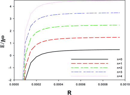
Figure 4: Plot of the energies versus the radius $R$ with different Landau indices $n$, in a curved sample of Eq.(28); here, $e=1.602\times 10^{-19}C,m=9.109\times 10^{-31}kg,c=3\times 10^{8}m/s,\hbar=1.055\times 10^{-34}J.s,k=1.75\times 10^{11}C.T/kg,B=1T.$ The energy levels have an asymptotic behavior as the radius $R$ increases. In the limit $R\rightarrow\infty$ they become the landau levels which in the planar case are dispersionless.

References

- [1] R. C. T. da Costa, Phys. Rev. A 23 (1982) 1981.
- [2] M. Encinosa and B. Etemadi, Phys. Rev. A 58 (1998) 77.
- [3] L. Kaplan, N. T. Maitra and E. J. Heller, Phys. Rev. A 56 (1997) 2592.
- [4] D. J. Struik, Lectures on Classical Differential Geometry, Dover Publications, 1988.
- [5] B. O’Neill, Elementary Differential Geometry, Academic Press, 1966.
- [6] J. E. Muller, Phys. Rev. Lett. 68 (1992) 385.
- [7] G. Ferrari, A. Bertoni, G. Goldoni and E. Molinari, Phys. Rev. B 78 (2008) 115326.
- [8] V. Atanosov, R. Dandoloff, Phys. Lett. A 371 (2007) 118.
- [9] A. V. Chaplik and R. H. Blick, New.J. Phys 6 (2004) 33.
- [10] I. Barke, R. Bennewitz, J.N. Crain, S.C.Erwin, A. Kirakosian, J.L. McChesney, F.J. Himpsel, Solid State Commun. 142 (2007) 617.
- [11] V. Atanasov, R. Dandoloff and A. Saxena Phys. Rev. B 79 (2009) 033404.
- [12] R. Dandoloff, A. Saxena, B. Jensen, Phys. Rev. A 81 (2010) 014102.
- [13] V. Atanasov and A. Saxena, Phys. Rev. B 81 (2010) 205409.
- [14] K. V. R. A. Silva, C. F. de Freitas and C. Filgueiras, Eur. Phys. J. B 86 (2013) 147.
- [15] A. Lorke, S. Bohm and W. Wegscheider, Superlattices and Microstruct. 33 (2003) 347.
- [16] C. L. Foden, M. L. Leadbeater, J. H. Burroughes and M. Pepper, J. Phys. Condens. Matter 6 (1994) L127.
- [17] C. L. Foden, M. L. Leadbeater and M. Pepper, Phys. Rev. B 52 (1995) R8646.
- [18] L. I. Magarill, D. A. Romanov and A. V. Chaplik, JETP Lett. 64 (1996) 460.
- [19] A. V. Chaplik, L. I. Magarill and D. A. Romanov, Physica B 249-251 (1998) 377.
- [20] A. V. Chaplik, L. I. Magarill and D. A. Romanov, Phys. Low-Dim. Struct. 1-2 (1998) 17.
- [21] M. L. Leadbeater et al., Phys. Rev. B 52 (1995) R8629.
- [22] E. Yablonovitch, D. M. Hwang, T. J. Gmitter, L. T. Florez and J.P. Harbison, Appl. Phys. Lett. 56 (1990) 2419.
- [23] P. Demeester, I. Pollentier, P. de Dobbelaere, C. Brys and P.Van. Daele, Semicond. Sci. Technol. 8 (1993) 1124.
- [24] G. J. Meyer, N. L. Dias, R. H. Blick and I. Knezevic, IEEE Trans. Nanotechnol 6 (2007) 446.
- [25] G. Ferrari, G. Cuoghi, Phys. Rev. Lett. 100 (2008) 230403.
- [26] C. Filgueiras, B. F. de Oliveira, Ann. Phys. (Berlin) 523 (2011) 898.
- [27] A. Oberlin, M. Endo and T. Koyama, J. Cryst. Growth 32 (1976) 335.
- [28] S. Iijima, Nature 354 (1991) 56.
- [29] L. I. Magarill, A. V. Chaplick and M. V. Entin, Phys. Usp 48 (2005) 953.
- [30] B. Jensen and R. Dandoloff, Phys. Lett. A 375 (2011) 448.
- [31] C. Filgueiras, E.O. Silva and F. M. Andrade, J. Math. Phys. 53 (2012) 122106.
- [32] Y. Aminov, Differential Geometry and Topology of Curves, CRC Press, 2000.