Review of Extreme Multilabel Classification
Abstract
Extreme multilabel classification or XML, is an active area of interest in machine learning. Compared to traditional multilabel classification, here the number of labels is extremely large, hence, the name extreme multilabel classification. Using classical one versus all classification wont scale in this case due to large number of labels, same is true for any other classifiers. Embedding of labels as well as features into smaller label space is an essential first step. Moreover, other issues include existence of head and tail labels, where tail labels are labels which exist in relatively smaller number of given samples. The existence of tail labels creates issues during embedding. This area has invited application of wide range of approaches ranging from bit compression motivated from compressed sensing, tree based embeddings, deep learning based latent space embedding including using attention weights, linear algebra based embeddings such as SVD, clustering, hashing, to name a few. The community has come up with a useful set of metrics to identify correctly the prediction for head or tail labels.
Keywords: extreme classification, head and tail labels, compressed sensing, deep learning, attention
1 Introduction
Extreme multilabel classification (XMC or XML) is an active area of research. It is multilabel classification problem, where the number of labels are very large going sometimes up to millions. The traditional classifiers such as one-vs-all, SVM, neural networks, etc, cannot be applied directly due to two major reasons. Firstly, the large number of labels creates a major bottleneck as it is not possible to have a simple classifier for each label due to memory constraints. Secondly, the presence of some labels which have very few samples in their support make learning about these labels a challenge. These kinds of labels are called tail labels and they will be a major problem which several methods will specially focus on.
This XML comes up in several contexts, such as finding appropriate tags for a Wikipedia page from the title or the full document, finding other items which are frequently bought together from the name or description of the item and finding appropriate tags for Ads from the Ad description. These are all real-time applications, thus, memory and time constraints are an extremely important factor in developing XML algorithms.
| Notation | Meaning |
|---|---|
| The set of real numbers | |
| Rounds the argument to 0 or 1 | |
| Frobenius norm of the argument | |
| Trace norm of the argument | |
| Norm of the argument | |
| Identity matrix of appropriate dimension | |
| Matrix containing the first columns of the identity matrix | |
| Pseudo-inverse of | |
| Trace of the matrix | |
| Transpose of the matrix | |
| Inverse of the matrix | |
| Natural logarithm of the argument | |
| The empty set | |
| Jacobian of with respect to | |
| Hessian of with respect to | |
| First columns of matrix | |
| Rank of matrix | |
| Cardinality of the set | |
| Stack the columns of matrix to get a vector | |
| Number of non zero entries in the matrix | |
| Expected value of the random variable | |
| AUPRC | Area under the precision-recall curve |
| i.i.d | Independent and identically distributed |
| CG | Conjugate Gradient Method |
2 Problem Formulation and Important Definitions
Though different papers in XML use different notation, recent papers consistently use the following notation which will be followed in this review paper too. The features are represented by the matrix where is the number of samples or instances, and represents the the dimension of the features. The label matrix is represented by where represents the total number of labels. Here represents that the th sample contains th label as ground truth. Individual features and labels for a sample is represented by and where represents the sample in consideration. The complete dataset is hence represented by .
Some other notation that appear several times are:
-
1.
which generally defines the dimension of the embedded space or the number of children in a tree.
-
2.
which generally depicts a linear learner.
-
3.
which represents the compression matrix for mapping features from the original or the embedded space.
These terms have been kept consistent throughout the paper, but have been redefined in the context if it conflicts with a previous definition.
Ranking:
The problem of extreme classification requires the model to predict a set of labels, which will be relevant to the given test sample. However, most models do not produce binary results, instead, they provide a relevance score based ranking for which labels are most likely according to the score. The exact labels, if required, can be selected using a thresholding based on the confidence. Thus, XML can be conceived of a ranking based problem instead of a classification problem. Even the most common metrics used in XML expect a ranking based output from the algorithm.
Head and Tail Labels:
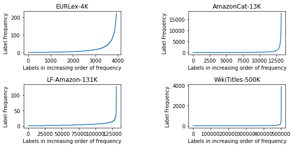
The number of samples are not evenly distributed among the labels in a typical XML problem. For example, in the Wiki-500K dataset Bhatia et al. (2016), 98% of labels have less than 100 training instances. Thus, some of the labels have enough data for the models to learn while most do not have enough data. These are called head and tail labels respectively. Most models trained directly without keeping the data distribution in mind are likely to develop an implicit bias towards the head labels. Thus, tail-label based metrics are an useful tool for measuring the effectiveness of a model.
3 Datasets and Metrics
3.1 Datasets
There are different kinds of datasets which are used for bench-marking XML results. One set of datasets is obtained from Amazon reviews and titles scraped from internet archives. The reviews, titles and product summary are used for prediction of the correct product tags McAuley and Leskovec (2013), McAuley et al. (2015b) and McAuley et al. (2015a). Wikipedia based datasets are used for prediction of tags on Wikipedia articles using the article or just the titles Zubiaga (2012). The dataset EurLex formulates large scale multilabel classification problems European legislature legal documents Loza Mencía and Fürnkranz (2008). Other proprietary datasets such as that of advertisement bids on bing are used by some methods.
3.2 Metrics
The following metrics are defined on the predicted score vector and ground truth label vector
Precision@k:
The most commonly used metric for measuring the performance of XML algorithms is P@. Here P@ measures what fraction of the top- predicted labels are present in the actual set of positive labels for the test data point. Formally, P@ is represented by
DCG@k and nDCG@k:
Discounted Cumulative Gain (DCG) and Normalized Discounted Cumulative Gain (nDCG) are common metrics for measuring the performance of a ranking system. Here DCG@ measures how much the ground truth scores of each of the top labels predicted by the algorithm add up to. A log term for the positions is added to ensure that better ordering is rewarded. Here nDCG@ is a modified version of the same metric which makes sure that the final score is well bounded for better comparison.
Propensity Based Metrics:
Jain et al. (2016) proposes a version of all the above metrics which take into account the fact that tail label predictions are performed well. The value represents the propensity score of label which ensures that the label bias is removed. This prevents models from achieving a high score from just correctly predicting head labels and completely ignoring tail labels. The corresponding versions of the metrics P@, DCG@ and nDCG@ are called PSP@, PSDCG@ and PSnDCG@.
4 Review
There are several categories of methods for performing extreme classification. We have broadly divided them into four categories based on the basic philosophy of the algorithm.
4.1 Compressed Sensing
The methods in this category are based on the concept of compressing the label space into a smaller, more manageable embedding space. The idea behind this method comes from signal-processing, where the compressed sensing technique can be used for signal reconstruction from much fewer samples than required, due to the sparsity. In the extreme multi-label scenario, the idea is to recover the original labels from predictions in a smaller label space. Again, The compression operation is valid due to the sparsity of the original label space.
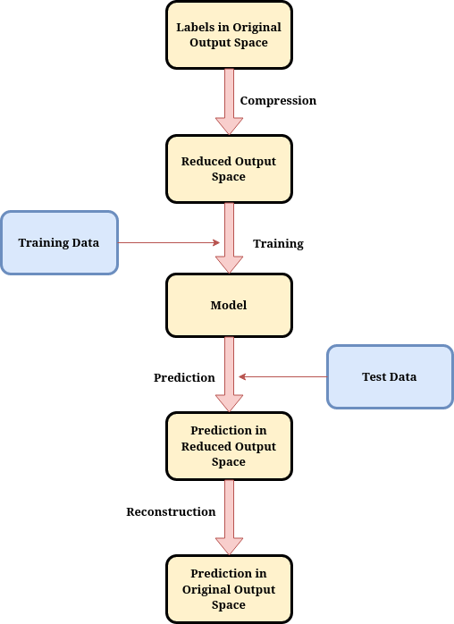
Broadly, there are 3 steps in this procedure -
-
1.
Compression: The original label space is compressed into a smaller vector space. This method of compression can use a simple linear transformation using an orthogonal matrix, hashing functions, clustering based approaches etc.
-
2.
Learning: Since after compression, the output space is much smaller, methods like binary relevance (predicting each element in the output space individually using a binary classifier) become viable.
-
3.
Reconstruction: During prediction, the output in the compressed space must be converted back to the original label space. This can be done using methods such as solving optimization algorithms, using inverse projection matrices, subset prediction algorithms etc.
The paper Hsu et al. (2009) was the first to make use of this technique. The application of compressed sensing in the XML problem was motivated from the observation that even though the label space of multi-label classification may be very high dimensional, the label vector for a given sample is often sparse. This sparsity of a label vector is be referred to as the output sparsity. The proposed method utilizes the sparsity of rather than that of . may be sparse but may have a large support. This may happen if there are many similar labels.
The proposed method proceeds in three steps. First, it compresses to where using a random compression matrix where is determined by the required sparsity level . It is ensured that is logarithmic with respect to . Next, for , a function is learnt to predict for every sample . Finally, during prediction, for an input vector , compute Then solve an optimization problem for finding a -sparse vector such that is closest to by some pre-defined metric.
The goal of the problem is to learn a predictor such that the error is minimized. The label space dimension is very large but of the corresponding label vector is -sparse. Given a sample we obtain a compressed sample and then learn a predictor with the objective of minimizing the error Then, the prediction can be obtained by composing the predictor of with a reconstruction algorithm The algorithm maps the predictions of compressed labels to predictions of in the original output space. This mapping is done by finding a sparse vector such that closely approximates the compressed labels
The compression step can be ensured to give a close approximation of the original feature vector if the compression matrix maintains certain isometry properties as explained in the paper. For the reconstruction algorithm, a greedy sparse compressed sensing reconstruction algorithm called Orthogonal Matching Pursuit (OMP) is used, first proposed in Pati et al. (1993).
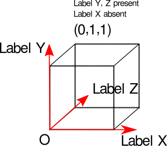
The previously stated method reduces the feature space significantly, enabling the method to train efficiently on large number of labels, but solving an optimization problem using OMP everytime during prediction is expensive. In the paper Tai and Lin (2012), a method is proposed which performs label space reduction efficiently and handles fast reconstruction. An SVD based approach is adopted for finding an orthogonal projection matrix which captures the correlation between labels. This allows easier reconstruction using the transpose of the projection matrix. The paper also uses a hypercube to model the label space of multi-label classification. It shows that algorithms such as binary relevance (BR, also called one-vs-all), compressive sensing (CS) can also be derived from the hypercube view.
The hypercube view aims to represent the label set of a given sample using a vector where iff component of is 1. As shown in Figure 3 (with ), each vertex of an -dimensional hypercube represents a label set . Each component of corresponds to one axis of a hypercube, which indicates the presence or absence of a label in
One vs All classification (also called Binary Relevance) and the Compressed Sensing Methods discussed can be formulated to be operations on this hypercube. The Binary Relevance method can be interpreted as projecting the hypercube into each of the dimensions before predicting. Using the hypercube view, each iteration of CS can be thought of as projecting the vertices to a random direction before training. Since this new subspace is much smaller than the original space that the hypercube belongs to.
Using the hypercube view, each iteration of CS can be thought of as projecting the vertices to a random direction before training. Since this new subspace is much smaller than the original space that the hypercube belongs to. Thus, the label-set sparsity assumption, which implies that only a small number of vertices in the original hypercube are of relevance for the multi-label classification task, allows CS to work on a small subspace.
A framework called Linear Label Space Transformation (LLST) is proposed by the paper, which focuses on a -dimensional subspace of instead of the whole hypercube. Each vertex of the hypercube is encoded to the point in the -dimensional space by projection. Then, a multi-dimensional regressor is trained to predict . Then, LLST maps back to a vertex of the hypercube in using some decoder . LLST basically gives a more formal definition to compressed sensing based methods in the XML context, although it assumes that the compression step must be linear.
The choice of the decoder depends on the choice of projection . For BR, we can simply take as the projection, and as the component-wise round(.) function. For CS, the projection matrix, , is chosen randomly from an appropriate distribution and , the reconstruction algorithm involves solving an optimization problem for each different .
Taking advantage of the hypercube sparsity in large multi-label classification datasets, we can take for the LLST algorithm, which in turn will reduce the computational cost. The proposed Principle Label Space Transformation (PLST) approach seeks to find the projection matrix and the decoder for such an -dimensional subspace through SVD. This method is described below.
The label sets of the given examples are stacked together to form a matrix such that each column of the matrix is one of the occupied vertices of the hypercube. The matrix is then decomposed using SVD such that
| (1) |
Here, is a unitary matrix whose columns form a basis for , is a diagonal matrix containing the singular values of and is also a unitary matrix. Assume that the singular values are ordered
The second line in (1) can be seen as a projection of using the projection matrix If we consider the singular vectors in corresponding to the largest singular values, we obtain a smaller projection matrix that maps the vertices to The projection matrix using the principle directions guarantees the minimum encoding error from to Because is an orthogonal matrix, we have Thus, can be used as a decoder to map any vector to Subsequently, a round based decoding is done to get the label vector. To summarize, first PLST performs SVD on and obtain , and then runs LLST with as . The decoder now becomes
PLST only considers labl-label correlations during the label space dimensionality reduction (LDSR). In the paper nan Chen and tien Lin (2012), a LSDR approach is explored which takes into account both the label and the feature correlations. The claim is that, such a method will be able to find a better embedding space due to the incorporation of extra information. The paper also provides an upper bound of Hamming loss, thus providing theoretical guarantees for both PLST and the proposed method, conditional principal label space transformation (CPLST). The method uses the concept of both PLST and Canonical Correlaion Analysis (CCA) to find the optimal embedding matrix.
Let such that where is the estimated mean of the label set vectors. Let be a projection matrix, is the embedded vector of . Let be the regressor to be learned such that , for a sample Let the predictions be obtained as with having orthogonal rows. In this setting, for round based decoding and orthogonal linear transformation , the Hamming loss is bounded by
| (2) |
Canonical Correlation Analysis (CCA) is a method generally used for feature space dimensionality reduction (FSDR). In the context of this method, it can be interpreted as feature aware Label Space Dimensionality Reduction (LSDR). The CCA is utilized for analysis of linear relationship between two multi-dimensional variables. It finds two sets of basis vectors and such that the correlation coefficient between the canonical variables and is maximized, where .
A different version of the algorithm, called Orthogonally Constrained CCA (OCCA) preserves the original objective of CCA and specifies that must contain orthogonal rows to which round based decoding can be applied. Then, using the hamming loss bound (2), when and OCCA minimizes in (2). That is, OCCA is applied for the orthogonal directions that have low prediction error in terms of linear regression.
After some simplification, the objective for OCCA becomes
| (3) |
where .
Thus, for minimizing the objective in (3) we only need the eigenvectors corresponding to the smallest eigenvalues of , or the eigenvectors corresponding to the largest eigenvalues of .
It can be seen that OCCA minimizes the prediction error in the Hamming Loss bound (2) with the the orthogonal directions that are relatively simpler to learn in terms of linear regression. In contrast, PLST minimizes the encoding error of the bound (2) with the “principal” components. The two algorithms OCCA and PLST can be combined to minimize the two error terms simultaneously with the “conditional principal” directions. Then, the optimization problem becomes
| (4) |
This problem can be solved by taking the eigenvectors with the largest eigenvalue of as the rows of . This minimizes the prediction error as well as the encoding error simultaneously. This obtained P is useful for the label space dimensionality reduction. The final CPLST algorithm is described below.
While CPLST provides a good bound on the error and shows theory behind the matrix compression based methods, it does not perform very well and also takes considerable time for prediction.
The paper Cissé et al. (2013), takes a novel approach to multilabel classification problem. The concept of Bloom filters Bloom (1970) is used to reduce the problem to a small number of binary classifications by representing label sets as low-dimensional binary vectors. However, since a simple bloom filter based approach does not work very well, the approach designed in this paper uses the observation that many labels almost never appear together in combination with Bloom Filters to provide a robust method of multi-label classification.
Bloom Filters are space efficient data structures which were originally designed for approximate membership testing. Bloom Filter (BF) of size uses hash functions, where each one maps from number of labels to , which are denoted as for . The value of is random and chosen uniformly from . Each of the hash functions define a representative bit of the entire bit vector of size . The bit vector of a label is obtained by concatenating all . There are at most non-zero bits in this bit vector. A subset is represented by a bit vector of size , defined by the bitwise-OR of the bit vectors of each of the labels in . The Bloom Filter predicts if the label is present in the set or not, by testing if the encoding of the set contains at all the representative bits of the label’s encoding. If the label is present, the answer is always correct, but if it is not present, there is a chance of a false positive.
Bloom filters can be naively applied to extreme classification directly. Let be the number of labels. Each individual label is encoded into a -sparse bit vector of dimension such that , and a disjunctive encoding of label sets (bit-wise-OR of the label codes that appear in the label set) represents the encoding of the entire label set. For each of the bits of the coding vector, one binary classifier is learned. Thus, the number of classification tasks is reduced from to . If , the individual labels can be encoded unambiguously on far less than bits. Also, the classifiers can be trained in parallel independently. However, standard BF is not robust to errors in the predicted representation. Each bit in the BF is represents multiple labels of the label set. Thus, an incorrectly prediction of a bit, may cause inclusion (or exclusion) of all the labels which it represents from the label set.
This problem can be tackled by taking into consideration the fact that the distribution of the label sets for real world datasets is not uniform. If it is possible to detect a false positive from the existing distribution of labels, then we can correct it. For example, if is the set of labels and is a false positive given then can be detected as a false positive if it is known that never appears together with the labels in . Thus, this method uses the non-uniform distribution of label sets to design the hash functions and a decoding algorithm to make sure that any incorrectly predicted bit has a limited impact on the predicted label set.
This paper develops a new method called the Robust Bloom Filter (RBF) which utilizes the fact that in most real-world datasets, many pairs of labels do not occur together, or co-occur with a very small probability. This allows it to improve over simple random hash functions. This is done in two ways, clustering and error correction.
During label clustering, the label set is partitioned into subsets such that clusters are mutually exclusive , i.e., no target set of a sample contains labels from more than one of each of the clusters . If the disjunctive encoding of Bloom filters is used, and if the hash function are designed such that the false positives for every label set can be detected to be mutually exclusive of the other labels. The decoding step can then detect this and perform correction on the bit. If for every bit, the labels in whose encodings it appears is mutually exclusive, then we can ensure a smooth decoding procedure. More clusters will result in smaller encoding vector size , which will result in fewer number of binary classification problems. Further, the clustering is performed after removing head labels, as they co-occur too frequently to divide into mutually exclusive subsets. For finding the label clustering, the co-occurrence graph is built, and the head labels are removed using the degree centrality measure (Degree Centrality is defined as the number of edges incident on a vertex). The remaining labels are then clustered using the Louvain Algorithm Blondel et al. (2008). The maximum size of each cluster is fixed to control the number of clusters.
As the second step, assuming that the label set is partitioned into mutually exclusive clusters (after removing the head labels), given a parameter , we can construct the required -sparse encodings by following two conditions: (1) two labels from the same cluster cannot share any representative bit (2) two labels from different clusters can share at most representative bits, ie. they cannot have the exact same encoding. Let denote the number of hash functions, denote the size of the largest cluster, denote the number of bits assigned to each label such that , and For a given which is the -th batch of successive bits, bits are used for encoding the -th label of each cluster. In this way, the first condition is satisfied. Also, this encoding can be used for labels. Now, for a given batch of bits, there are different subsets of bits. Thus, we can have at most label clusters. The labels (one from each cluster) are injectively (one-one) mapped to the subsets of size to define the representative bits of these labels. Thus, these encoding scheme satisfies condition 2 as no two subsets in shares more than indexes. Using a BF of size we have -sparse label encodings that satisfy the two conditions for labels partitioned into mutually exclusive clusters of size at most In terms of compression ratio this encoding scheme is most efficient when the clusters are perfectly balanced, and the number of partitions is exactly equal to for some An implementation of this scheme is shown in Table 2 (for bits, clusters, representative bits and ).
| bit index | representative for labels | bit index | representative for labels |
|---|---|---|---|
| cluster index | labels in cluster | cluster index | labels in cluster |
|---|---|---|---|
During the prediction procedure, given an sample and the encoding predicted , the predicted label set is computed by a two-step process. Firtsly, cluster identification is performed by picking whichever cluster has maximum number of representative bits, and close to the number of representative bits close to that of . Secondly, the correctl labels within the cluster are found by using probabilistic sampling under the assumption that whichever label in the cluster has the most representative bits in common with is the most likely to occur. If logistic regression is used as base learners for binary classification, the posterior probabililty can be used for computing the cluster scores instead of the binary decisions. The cluster which maximizes the cluster score is chosen. The advantage of using a randomized prediction for the labels is that a single incorrectly predicted bit does not result in too many predicted labels.
The paper also provides some theoretical bounds on the error by deriving that each incorrectly predicted bit in the BF cannot imply more than two incorrectly predicted labels. However, R-BF still does not show very good results, probably due to the assumption that labels from different clusters will never co-occur, which highly limits the output space.
The paper Jasinska and Karampatziakis (2016) also takes a similar approach to encoding the labels. A method called Log Time Log Space Extreme classification (LTLS) is proposed which transforms the multi-label problem with labels into a structured prediction problem by encoding the labels as edges of a trellis graph. This enables inference and training in order which is logarithmic in the number of labels along with reduced model size.
First, a trellis graph with steps is built, each with states, a root, and a sink vertex as shown in the figure 4. There are edges in the graph. A path from the root to the sink is a vector of length . There are paths in the graph. Each label , , is assigned to path . Additional edges are used if the number of labels is not power of . This step is equivalent to binary encoding of number of labels. The number of edges . Each edge in the above trellis corresponds to a function we learn. For a label , the encoding vector has at places where the edge is part of the corresponding path , or has otherwise.
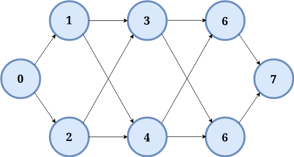
During prediction, given an input , the algorithm predicts values from each of the binary classifiers. The value at each edge is a function which can be assumed to be a simple linear regressor. The score of label is the sum of values in the path .
| (5) |
For prediction of the final labels from the label scores, we can use the scheme where top-k labels correspond to longest paths in the trellis graph (which can be found using DP based list Viterbi algorithm Seshadri and Sundberg (1994)).
Despite the unique approach, the algorithm failed to give very high scores compared to emerging tree based and linear algebra based methods. Subsequent work was done by Evron et al. (2018) which attempted different graph structures, but it was only applicable for multi-class classification.
Although Cissé et al. (2013) uses hashing based label space compression technique, it makes assumptions about the co-occurrence of label which leads to reduction in performance. The paper Medini et al. (2019), proposes Merged Averaged Classifiers via Hashing (MACH) which is a hashing based approach to XML which utilizes something similar to a count sketch data structure instead of bloom filters for performing universal hashing. This reduces the task of extreme multi-label classification to a small number of parallelizable binary classification tasks.
Sketch Charikar et al. (2002) is a data structure that stores a summary of a dataset in situations where the whole data would be prohibitively costly to store. The count-sketch is a specific type of sketch which is used for counting the number of times an element has occurred in the data stream. Let be a stream of queries, where each which is the set of objects queried. Let be hash functions from to . Count sketch data structure consists of these hash functions along with a array of counters , where is the number of hash functions and is the number of buckets for each hash table. There are two supported operations: (1) Insert new element into sketch , which is performed by adding for each hash function at position (2) Count the number of times element has occurred, performed by where can be mean, median or minimum.
If we use only one hash function, then we get the desired count value in expectation but the variance of the estimates is high. To reduce the variance, hash functions are used and their outputs are combined. This concept is utilized by the proposed method.
The method Merged-Averaged Classifiers via Hashing (MACH) randomly merges classes into random-meta-classes or buckets using randomized hash functions. This merging of labels into meta classes gives rise to a smaller multi-label classification problem and classifiers such as logistic regression or a deep network is used for this meta-class classification problem. Let be the number of hash functions. Then, the classification algorithm is repeated independently for times using an independent 2-universal hashing scheme each time. During prediction, the outputs of each of the classifiers is aggregated to obtain the prediction class (The aggregation scheme may be median, mean or min). This is the step where an estimate like method of the count sketch data structure is used. The advantage of MACH stems from the fact that since each hash function is independent, training the classifiers are trivially parallelizable. The parameters and can be tuned to trade accuracy with both computation and memory.
The algorithms are described below.
The paper is able to prove a bound on the error due to the theorem that if a pair of classes is not indistinguishable, then there is at least one classifier which provides discriminating information between them. If the loss function used is softmax, then we get the multiclass version of MACH. For a multilabel setting, the loss function can be binary cross-entropy.
Comparison between above stated methods
- 1.
-
2.
CPLST nan Chen and tien Lin (2012) outperforms PLST but is much slower and less scalable.
- 3.
| Compressed Sensing Based Methods | |||
|---|---|---|---|
| Algorithm | Compression | Learning | Reconstruction |
| CS | Compression Matrix obtained from compression methods such as OMP | Simple regressors in the reduced space | Solving an optimization problem |
| PLST | Compression matrix obtained from SVD | Simple regressors in the reduced space | Round based decoding after multiplying with transpose of compression matrix |
| CPLST | Compression matrix obtained from a combination of OCCA and PLST, considering both feature-label and label-label correlations | Simple regressors in the reduced space | Round based decoding after multiplying with transpose of compression matrix |
| R-BF | Ecodes every subset of labels into a bit encoding by ’OR’ operation on individual labels | Binary Classifiers for each bit in encoding | An algorithm based on identification of the closest labels included within the predicted encoding |
| LTLS | Each label is assigned to a path in a trellis graph and a corresponding bit vector is obtained | Regressors at each edge predict the weight of the edges | Longest path algorithms are used to find the top k paths and corresponding labels are predicted |
| MACH | Universal hash functions are used to assign each label a bucket. Multiple hash functions are used to iterate the process. | Multi label classifiers are used to predict the corresponding meta labels for each hash function | A sketch-like aggregation function is used to find the predicted labels from the predicted meta-labels |
4.2 Linear Algebra
The methods in this category do not follow any specific structure, but are heavily reliant on simple Linear Algebra based optimizations, which allow the methods to gain an advantage over simply embedding in a lower dimensional space like in compressed sensing based methods. The methods may end up working like compressed sensing ones, but generally aim to do some improvement over them. For example, LEML converts the entire process of compression, prediction and decoding in CPLST to one step directly and proves the equivalence. SLEEC on the other hand refutes the usage of the low-rank assumption used in most of the embedding methods and develops a KNN based distance preserving embeddings. PD-SPARSE develops a method for optimizing the XML problem in both primal and dual spaces and obtain sparse embeddings. A summary of each method is provided at the end of the section.
Subset-selection is one of the most common methods utilized to make the extreme classification problem tractable. The core idea was to find a good representative subset of labels on which a simple classifier can be learnt and the predictions can be scaled back to the full label set. The paper Bi and Kwok (2013) performs a subset selection on the labels to form a smaller label space which approximately spans the original label space. The labels are selected via a randomized sampling procedure where the probability of a label being selected is proportional to the leverage score of the label on the best possible subset space.
Balasubramanian and Lebanon (2012) has previously attempted the label selection procedure. This paper assumes that the output labels can be predicted by the selected set of labels. It solves an optimization problem for selecting the subset. However, the size of the label subset cannot be controlled explicitly and also the optimization problem quickly becomes intractable. To address this issue, this paper models the label subset selection problem as a Column Subset Selection Problem (CSSP).
The method Column Subset Selection Problem (CSSP) seeks to find exactly columns of such that these columns span as well as possible, given a matrix and an integer . For this purpose, an index set of cardinality is required such that is minimized. Here, denotes the sub-matrix of containing the columns indexed by and is the projection matrix on the -dimensional space spanned by the columns of In Boutsidis et al. (2009), this problem is solved in two stages : a randomized stage and a deterministic stage. Let denote the transpose of the matrix formed by the top right singular vectors of In the randomized stage, a randomized column selection algorithm is used to select columns from Each column of is assigned a probability which corresponds to the leverage score of the column of on the best rank subspace of It is defined as The randomized stage of the algorithm samples from the columns of using this probability distribution. In the deterministic stage, a rank revealing QR (RRQR) decomposition is performed to select exactly columns from a scaled version of the columns sampled from
In the extreme classification setting, the objective of the label subset selection problem can be stated as
| (6) |
The approach proposed in this paper directly selects the columns of the label matrix The algorithm is given in Algorithm 5. First, a partial SVD of is computed to pick the top right singular vectors, Then, the columns in are sampled with replacement, with the probability of selecting the column being However, instead of selecting columns, the sampling procedure is continued until different columns are selected. It has been shown that if the number of trials is (which is in ) for some constants and then the algorithm gives a full rank matrix with high probability. Once the columns have been obtained, classifiers are learned.
The minimizer of the objective (6) satisfies
| (7) |
From (7), it can be seen that each row of can be approximated as the product of each row of with Now, given a test sample let denote the prediction vector. Then, using (7), the -dimensional prediction vector can be obtained as The elements of the -dimensional output vector are further rounded to get a binary output vector.
Empirical results show that ML-CSSP gives lower RMSE compared to other methods available at that time. The given CSSP algorithm is also compared to the two-stage algorithm of Boutsidis et al. (2009) and the results show that the number of sampling trials and encoding error is better for the proposed algorithm. As the number of selected labels is increased, training error increases as the number of learning problems increase while the encoding errors decrease as is increased, as expected. ML-CSSP is able to achieve lower training errors than PLST Tai and Lin (2012) and CPLST nan Chen and tien Lin (2012) as selected labels are easier to learn than transformed labels.
In the paper Yu et al. (2013), the problem of extreme classification with missing labels (labels which are present but not annotated) is addressed by formulating the original problem as a generic empirical risk minimization (ERM) framework. It is shown that the CPLST nan Chen and tien Lin (2012), like compression based methods, can be derived as a special case of the ERM framework described in this paper.
The predictions for the label vector are parameterized as where is a linear model. Let be the loss function. The loss function is assumed to be decomposable, i.e.,
The motivation for the framework used in this paper comes from the fact that even though the number of labels is large, there exists significant label correlations. This reduces the effective number of parameters required to model them to much less than which in turn constrains to be a low rank matrix.
For a given loss function and no missing labels, the parameter can be learnt by the canonical ERM method as
| (8) |
where is a regularizer. If there are missing labels, the loss is computed over the known labels as
| (9) |
where is the index set that represents known labels. Due to the non-convex rank constraint, this (9) becomes an NP-hard problem. However, for convex loss functions, the standard alternating minimization method can be used. For L2-loss, eq. (8) has a closed form solution using SVD. This gives the closed form solution for CPLST.
Most of the compressed sensing based methods and previous embedding based methods assume that the label matrix is low rank and aims to hence predict in a smaller dimensional embedding space rather than the original embedding space. The paper Bhatia et al. (2015) claims that the low-rank assumption is violated in most practical XML problems due to the presence of the tail labels which act as outliers and are not spanned by the smaller embedding space. Thus, this paper proposes a method called Sparse Local Embeddings for Extreme Multi-label Classification (SLEEC) which utilizes the concept of ”distance preserving embeddings” to predict both head and tail labels effectively.
The global low rank approximations performed by embedding based methods do not take into account the presence of tail labels. It can be seen that a large number of labels occur in a small number of documents. Hence, these labels will not be captured in a global low dimensional projection.
In SLEEC embeddings are learnt which non-linearly capture label correlations by preserving the pairwise distances between only the closest label vectors, i.e. only if where is a distance metric. Thus, if one of the label vectors has a tail label, it will not be removed by approximation (which is the case for low rank approximation). Regressors are trained to predict During prediction SLEEC uses kNN classifier in the embedding space, as the nearest neighbours have been preserved during training. Thus, for a new point , the predicted label vector is obtained using For speedup, SLEEC clusters the training data into clusters, learns a separate embedding per cluster and performs kNN only within the test point’s cluster. Since, clustering can be unstable in large dimensions, SLEEC learns a small ensemble where each individual learner is generated by a different random clustering.
Due to the presence of tail labels, the label matrix cannot be well approximated using a low-dimensional linear subspace. Thus it is modeled using a low-dimensional non-linear manifold. That is, instead of preserving distances of a given label vector to all the training points, SLEEC attempts to preserve the distance to only a few nearest neighbors. That is, it finds a dimensional matrix which minimizes the following objective:
| (10) |
where the index set denotes the set of neighbors that we wish to preserve, i.e., iff denotes the set of nearest neighbors of . is defined as :
| (11) |
The above equation, after simplification can be solved by using Singular Value Projection (SVP) Jain et al. (2010) using the ADMM Sprechmann et al. (2013) optimization method. The training algorithm is shown in Algorithm 6.
The paper Mineiro and Karampatziakis (2014) proposes a method called REMBRANDT, which utilizes a correspondence between rank constrained estimation and low dimensional label embeddings to develop a fast label embedding algorithm.
The assumption made by the paper is that with infinite data, the matrix being decomposed is the expected outer product of the conditional label probabilities. In particular, this indicates that two labels are similar when their conditional probabilities are linearly dependent across the dataset.
The label embedding problem is modeled as a rank constrained estimation problem, as described below. Given a data matrix and a label matrix , let the weight matrix to be learned have a low-rank constraint. In matrix form
| (12) |
The solution to (12) is derived in Friedland and Torokhti (2006). The equation is further simplified to obtain a low rank matrix approximation problem, which is solved using a randomized algorithm proposed in Halko et al. (2011).
After the predictions are done in the embedding space, a decoding matrix is used to project the predicted label matrix back to the space.
Yen et al. (2016) shows that for the extreme classification problem, a margin-maximizing loss with penalty, yields a very sparse solution both in primal and in dual space without affecting the predictor’s expressive power. The proposed algorithm, PD-Sparse incorporates a Fully Corrective Block Coordinate Frank Wolfe (FC-BCFW) Lacoste-Julien and Jaggi (2015) algorithm that utilizes this sparsity to achieve a complexity sublinear to the number of primal and dual variables. The main contribution of this method to the field is the use of the separation ranking loss in XML which was further used in several subsequent methods.
Instead of making structural assumption on the relation between labels, for each instance, there are only a small number of correct labels and the feature space can be used to distinguish between labels. Under this assumption, a simple margin-maximizing loss can be shown to yield sparse dual solution in the setting of extreme classification. When this loss is combined with penalty, it gives a sparse solution both in the primal as well as dual for any parameter .
Let denote positive label indexes and denote negative label indexes. In this paper, it is assumed that is small and does not grow linearly with .
The objective of separation ranking loss is to compute the distance between the output and the target. The loss penalizes the prediction on an input by the highest response from the set of negative labels minus the lowest response from the set of positive labels.
| (13) |
where an instance has zero loss if all positive labels have higher positive responses that that of negative labels plus a margin. Here .
In a binary classification scenario, the support labels are defined as
| (14) |
Here, the labels that maximize the loss in (13) form the set of support labels. The basic inspiration for use of loss (13) is that for any given instance, there are only a few labels with high responses and thus, the prediction accuracy can be boosted by learning how to distinguish between these labels. In the extreme classification setting, where is very high, only a few of them are supposed to give high response. These labels are taken as the support labels.
The problem now becomes to find a solution to the problem
| (15) |
It can be shown that the solutions in both the primal and dual space is sparse in nature. Thus, sparsity assumptions on are not hindrances but actually a property of the solution. The above formalized problem is solved by separating blocks of variables and constraints to use the Block Coordinate Frank Wolfe Algorithm Lacoste-Julien et al. (2013). The only bottleneck in the entire process comes down to how to find the most violating label in each step, for which an importance sampling based heuristic method is used.
In this paper Xu et al. (2016), the idea of using low-rank structure for label correlations is re-visited keeping in mind the tail labels. The claim made in Bhatia et al. (2015) which says that low-rank decompositions are not applicable in extreme classification is studied and a claim is made which says that low-rank decomposition is applicable after removal of tail labels from the data. Hence, in addition to low-rank decomposition of label matrix, the authors add an additional sparse component to handle tail labels behaving as outliers.
Assuming the label matrix as it is decomposed as
where is low rank and depict label correlations and is sparse, and captures the influence of tail labels. This can be modeled as
| (16) |
Given and , we wish to learn regression models such that and where . Let where We impose the constraints by
| (17) |
The objective (17) can be divided into three subproblems :
| (18) | |||
| (19) | |||
| (20) |
Each of these sub problems can be solved by equating the partial differentiation to zero.
The sub problems (18),(19) and (20) can be efficiently solved in parallel and their solutions can be combined to achieve the final solution. This is a divide and conquer strategy.
For the divide step, given the label matrix it is randomly partitioned into number of -column sub matrices where we suppose and each Thus, the original problem is divided into sub-problems regarding The basic optimization methods discussed in the previous section can now be adopted to solve these sub-problems in parallel, which outputs the solutions as
The conquer step exploits column projection to integrate the solutions of sub-problem solutions. The final approximation to problem (17) can be obtained by projecting onto the column space of After obtaining the objective can be optimized over each column of in parallel to obtain the sparse component of the resulting multi-label predictor.
In Tagami (2017), the author highlights some major problems that the SLEEC Bhatia et al. (2015) algorithm has. SLEEC uses only feature vectors for -means clustering. It does not access label information during clustering. Thus data points having the same label vectors are not guaranteed to be assigned to the same partition. As the number of partitions increase, the data points having the same tail labels may be assigned to different partitions. Further, in the prediction step, SLEEC predicts labels of the test point by using the nearest training points in the embedding space. Hence, the order of distance to the neighbors of the test point is considered, and not the values themselves. This may cause an isolated point which may be far from a cluster center to belong to that cluster.
The proposed method, AnnexML is able to solve these issues by learning a multi-class classifier, which partitions the approximate -Nearest Neighbor Graph (KNNG) Dong et al. (2011) of the label vectors in order to preserve the graph structure as much as possible. AnnexML also projects each divided sub-graph into an individual embedding space by formulating this problem as a ranking problem instead of a regression one. Thus the embedding matrix is not a regressor like in SLEEC.
There are mainly three steps to the training of the AnnexML algorithm. Firstly, AnnexML learns to group the data points that have similar label vectors to the same partition, which is done by utilizing the label information. It forms a -nearest neighbor graph (KNNG) of the label vectors, and divides the graph into sub-graphs, while keeping the structure as much as possible. After the KNNG has been computed and partitioned, we learn the weight vector for each partition such that the data points having the same tail labels are allocated in the same partition while the data points are divided almost equally among partitions. Thirdly, the learning objective of AnnexML is to reconstruct the KNNG of label vectors in the embedding space. For this task, it employs a pairwise learning-to-rank approach. That is, arranging the nearest neighbors of the -th sample is regarded as a ranking problem with the -th point as the query and other points as the items. The approach used is similar to DSSM Yih et al. (2011).
The prediction of AnnexML mostly relies on the -nearest neighbor search in the embedding space. Thus, for faster prediction, we need to speed up this NN search. An approximate -nearest neighbor search method is applied, which explores the learned KNNG in the embedding space by using an additional tree structure and a pruning technique via the triangle inequality. This technique gives AnnexML a much faster prediction than SLEEC.
In the paper Jalan and Kar (2019), a new method for reducing the dimensionality of the feature vectors is explored which is especially useful when the feature vector is already sparse. This is not a specific XML method but a add-on method for any XML algorithm which can be used to provide speedups when the number of features is very high with minimal loss of accuracy.
The reduction in dimensionality is performed by a method called feature agglomeration, where clusters of features are created and then a sum is taken to create new features. If is partition of the features , then corresponding to every cluster we create a single feature by summing up the features within cluster . Thus, for a given vector we create an agglomerated vector with just features using the clustering . The th dimension of will be for
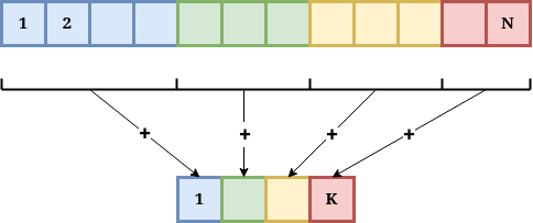
The proposed method, DEFRAG, clusters the features into balanced clusters of size not more than . If this results in clusters, then we sum up the features in these clusters to obtain -dimensional features which are subsequently used for training and testing using any XML method. It can be theoretically proven that with a linear classification method, feature agglomeration cannot give worse performance than the original method.
DEFRAG first creates a representation vector for each feature and then performs hierarchical clustering on them. At each internal node of the hierarchy, features at that node are split into two children nodes of equal sizes by solving either a balanced spherical 2-means problem, or by minimizing nDCG. This process is continued until we are left with less than features at a node, in which case the node is made a leaf. The representative vectors can be either based on features only or labels and features together which can perform different functions.
The use of DEFRAG for dimensionality reduction has several advantages over the classical dimensionality reduction techniques such as PCA or random projections for high-dimensional sparse data. Feature agglomeration in DEFRAG involves summing up the coordinates of a vector belonging to the same cluster. This is much less computationally expensive than performing PCA or random projections. Also, the feature agglomeration done in DEFRAG does not densify the vector. If the sparsity of a vector is , then the -dimensional vector resulting from the agglomeration will have at most non-zeros ( if one feature from each cluster has a non-zero). This is unlike PCA or random projections which densify the vectors which in turn cause algorithms such as SLEEC or LEML to use low dimensional embeddings. This results in a loss of information. Thus, using DEFRAG preserves much of the information of the original vectors and also offers speedup due to reduced dimensionality.
Comparison between above stated methods
-
1.
Method LEML outperforms all of the compressed sensing based methods in terms of performance and subsequent methods based on LEML hence outperform compressed sensing based methods.
-
2.
Method SLEEC was the first to find the issue with low-rank decomposition based methods proposed as compressed sensing based methods. Using a distance preserving embedding, SLEEC achieved a large improvement over previous methods. AnnexML improved on SLEEC further improving both performance and prediction times.
-
3.
Method REML revisits the idea of low-rank embeddings by separating out the tail labels and learning different predictors for head and tail labels.
| Linear Algebra Based Methods | ||
|---|---|---|
| Algorithm | Type of Method | Summary |
| MLCSSP | Subset Selection | The maximum spanning subset of the label matrix is chosen i.e., a label subset is chosen which best represents the entire label space. Prediction is performed in this label space and the results are then extrapolated on the entire label set. |
| LEML | Low rank decomposition | The low-rank decomposition of the label matrix is assumed and a general ERM framework is proposed to solve it. Attempts to generalize compressed sensing based methods like CPLST and apply them for missing labels too. |
| SLEEC | Distance preserving embeddings | A method for generating embeddings which preserve the distance between labels in the generated embedding space. The prediction is done via KNN in the embedding space. |
| REMBRANDT | Low rank decomposition | Uses a randomized low-rank matrix factorization based technique to perform rank-constrained embedding. It can be shown to be equivalent to CPLST in the simplest case. |
| PD-SPARSE | Separation Ranking Loss based Frank Wolfe | Utilizes the dual and primal sparsity of a solution to the problem with separation ranking loss and regularization. The problem is solved via a Fully Corrective Block Coordinate Frank Wolfe Algorithm. |
| REML | Low rank decomposition | Re-visits the Low rank decomposition technique and tries to resolve the issue tail labels create by separating head and tail labels. This makes the low-rank assumption valid once again and head and tail labels are predicted separately. |
| AnnexML | Distance preserving embedding | Distance preserving embeddings and improvement over the SLEEC algorithm by using a KNN graph for partitioning labels, using a ranking based loss and using an ANN based prediction technique. |
| DEFRAG | Feature Agglomeration Supplement | An algorithm for dealing with large feature spaces in extreme classification by performing feature agglomeration. Can also be used for feature imputation and label re-ranking. |
4.3 Tree Based
Tree Based methods rely on the inherent hierarchy of the data to speed up the multi-label learning and prediction. The main goal of these methods is to repeatedly divide either the label or sample space in order to narrow down the search space during prediction. The leaf nodes generally contain a one-versus-all or a simple averaging based technique for final prediction.
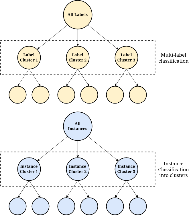
Broadly, these techniques can be categorized into two types :
-
1.
Label Partitioning based. These methods rely on dividing the labels into clusters at each level, thus forming a sort of meta-label structure. Each of the levels is then equipped with a multi-label classifier to determine the most relevant meta labels. The leaves contain a small number of labels which can be dealt with by a one-vs-all classifier.
-
2.
Sample/Instance Partitioning Based. These methods group together the train samples and cluster them into branches at each level. This forms a sort of decision tree structure which can be used to group the incoming test point into the correct branches and finally reach the leaf. The branch decisions are made by a multi-class classifier and the final predictions on the leaf are then made by combining the labels of the instances at that leaf.
Tree Based methods in general provide faster training and prediction than the embedding and deep-learning based methods due to the reduction of training and search space provided by the tree structure.
The paper Prabhu and Varma (2014) proposes a method called FastXML which improves upon the state of the art tree based multi label classification methods of the time, Multi-Label Random Forest Classifier (MLRF) Liu et al. (2015) and Label Partitioning by Sub-linear Ranking (LPSR)Weston et al. (2013). Both these methods learn a hierarchy of the labels to deal with the large number of labels. The LPSR learns relaxed integer programs to partition the sample into the clusters learnt by k-means like algorithm. MLRF on the other hand learn an ensemble of randomized trees but uses a brute force partitioning method based on Gini index or entropy. In contrast, FastXML learns to partition samples or data points rather than labels.
Both methods MLRF and LPSR did not perform competitively on XML datasets when compared with existing methods. Significantly higher accuracy is achieved by FastXML by optimizing a nDCG loss along with learning the ranking of the labels in each partition at the same time. An alternating minimization algorithm for efficiently optimizing the problem formulation is also developed.
FastXML proposes to learn the hierarchy by directly optimizing the ranking loss function. This way of learning the hierarchy is better as nDCG is a measure which is sensitive to both relevance and ranking ensuring that the relevant positive labels are predicted with the highest possible ranks. This is not guaranteed by rank insensitive measures such as Gini-index in MLRF or clustering error in LPSR.
FastXML partitions the current node feature space by learning a linear separator such that
where where represents indices of all the training points present at the node being partitioned. is indicative of whether point was assigned to the negative r positive partition . The positive and negative partition are represented by variables and respectively. User defined parameters and are used to determine the relative importance of the three terms.
There are three types of parameters in the equation, , and . Though the other two parameters can be obtained from itself, it is easier to optimize with separate parameters. The first term in the loss is an term on which ensures sparsity. The second term is the log loss of . This term optimizes the parameters and together, as the solution to be obtained is sign. This tries to make sure that a point which is assigned to the positive (negative) partition, i.e points for which will have positive (negative) values of . The third and fourth terms in the equation maximize the of the rankings predicted for the positive and negative partitions, and respectively. These terms relate to and thus to .
Maximizing nDCG makes it likely that the relevant positive labels for each point are predicted as high as possible. As a result, points within the same partition are more likely to have similar labels whereas points in different partitions are more likely to have dissimilar labels.
The loss also allows a label to be assigned to both partitions if some of the points which contain the label are assigned to the positive partition and some to the negative. This makes the FastXML trees more robust as the error which is propagated from the parents may be corrected by the children.
Once we have learned the hyperplane during the training phase, then we know how to partition a test instance into a left or a right child. So, now we know how to traverse the tree starting at the root and keep applying this procedure recursively until we get to a leaf.
Given a new data point for prediction, , FastXML’s top ranked predictions are given by
| (22) |
where is the number of trees in the FastXML ensemble and is the distribution of points in the lead nodes containing in tree . It is found empirically, that the proposed nDCG based objective function learns balanced which leads to fast and accurate predictions in logarithmic time. The main reason behind the accurate prediction is the novel node partitioning formulation which optimized an nDCG based ranking loss over all the labels. Such a loss turns is more suitable for XML than the Gini index used by MLRF or the clustering error used by LPSR and efficiently scales to problems with more than millions of labels.
In the paper Prabhu et al. (2018), a label tree partitioning based method, Parabel, is proposed which aims to achieve the high prediction accuracy achieved by one-vs-all methods such as DiSMEC Babbar and Schölkopf (2016) and PPDSparse Yen et al. (2017) while having fast training and prediction times. Parabel overcomes the problem of large label spaces by reducing the number of training points in each one vs all classifier such that each label’s negative training examples are those with most similar labels. This is performed using the tree structure learnt.
In Parabel, labels are recursively partitioned into two groups to create a balanced binary tree. After the partitioning, similar labels end up in a group. Partitioning is stopped when the leaf node contains at-least labels. After the tree construction, two binary classifiers have to be trained at each internal node. These two classifiers help in determining whether the test point has to be sent to left or the right child or both. At the leaf node One vs All classifiers are trained for each label associated with that leaf node. At the time of prediction, a test sample is propagated through the tree using classifiers at internal nodes, after reaching leaf nodes, ranking over the labels is assigned using the one vs all classifiers present at the leaf.
The labels are represented by the normalized sum of training instances to in which it appears. This label representation is used to cluster the labels using a -means objective along with an extra term to ensure that the label splits are uniform. Further, the distance between labels is measured using the cosine function, which basically leads to a spherical k-means objective with . This objective is solved using the well-known alternating minimization.
Using this splitting procedure recursively for each internal node of the tree starting from the root, we can partition the labels to create a balanced binary tree. Partitioning is stopped when there are less than number of labels in a cluster and they become leaf nodes. In the final tree structure we end up with, the internal nodes represent meta-labels, and the problem at each node becomes a smaller multi-label classification problem.
After the tree structure is learnt, we need to train a classifier at each edge for predicting the probability of the child being active given that the parent is active. Let be a binary variable associated with each node for each sample. For a given sample , if then the sub-tree rooted at node has a leaf node which contains a relevant label of the given sample. Thus we need to predict at each internal node, where represents a child of node . This can be done by optimizing the MAP estimate
| (23) |
which is parameterized by .
Similarly, at the leaf nodes one has to minimize the loss
| (24) |
which basically trains a one-vs-all classifier for each label present in that leaf.
Highly parallel and distributed versions of Parabel are possible because all the optimization problems are independent. The independence does not imply that model does not recognize label to label dependency or correlation. In fact, the model does take into account label-label correlation when clustering the labels. At the time of clustering similar labels are grouped into a cluster, thus model is not truly independent with respect to labels.
During prediction, the goal is to find the top labels with the highest value of
| (25) |
where is the parent of node This means that we have to find the path to the leaf from the root with the maximum value of product of probabilities on its nodes. We can use a beam search (greedy BFS traversal) to find the top labels with the highest probabilities.
The paper Siblini et al. (2018) proposes a random forest based algorithm with a fast partitioning algorithm called CRAFTML (Clustering based RAndom Forest of predictive Trees for extreme Multi-label Learning). The method proposed is also an instance/sample partitioning based method like FastXML but it uses a k-means based classification technique in comparison to nDCG optimization in FastXML. Another major difference with FastXML is that it uses -way partition in the tree instead of 2-way partitions. CRAFTML also exploits a random forest strategy which randomly reduces both the feature and the label spaces using random projection matrices to obtain diversity.
CRAFTML computes a forest of -ary instance trees which are constructed by recursive partitioning. The base case of the recursive partitioning is either of the three the number of instances in the node is less than a given threshold all the instances have the same features, or all the instances have the same labels. After the tree training is complete, each leaf stores the average label vector of the samples present in the leaf.
The node training stage in CRAFTML is decomposed into three steps. First, a random projection of the label and feature vectors into lower dimensional spaces is performed. This is done using a projection matrix which is randomly generated from either Standard Gaussian Distribution or sparse orthogonal projection. Next, -means is used for recursively partitioning the instances into temporary subsets using their projected label vectors. We thus obtain cluster centroids. The cluster centroids are initialized with the -means++ strategy which improves cluster stability and algorithm performances against a random initialization. Finally, the cluster centroids are re-calculated by taking the average of feature vectors assigned to the temporary clusters. We now have a -means classifier which is capable of classification by finding the closest cluster to any instance. The instances are partitioned into final subsets (child nodes) by the classifier.
The training algorithm is given below.
During prediction, we traverse from the root to the leaves using the -means classifier decisions at each layer. Once a leaf is reached, prediction is given by the average of the label vectors of instances present at that leaf. Using the forest, we aggregate the predictions which largely helps increase the accuracy.
Khandagale et al. (2020) introduces a method Bonsai, which improves on Parabel Prabhu et al. (2018). The authors make the observation that in Parabel, due to its deep tree structure there is error propagation down the tree, which means that the errors in the initial classifiers will accumulate and cause higher classification error in leaf layers. Also, due to the balanced partitioning in the tree layers, the tail labels are forced to be clustered with the head labels, which causes the tail labels to be subsumed. Hence, in Bonsai, a shallow tree structure with children for each node is proposed which () prevents ”cascading effect” of error in deep trees. () allows more diverse clusters preventing misclassification of tail labels.
Another contribution of the paper is to introduce different types of label representations based on either the feature-label correlations , label-label co-occurrence or a combination of both.
Let be the given training samples with and . , are data and label matrices respectively. Let be the representation of label
There are three ways to represent the labels before clustering.
In the input space representation, , this can be compactly written as , where each row corresponds to the label representation of the label, i.e. row is the label representation of label number ().
| (26) |
In the output space representation, the Label representation matrix is given by
| (27) |
In the joint input-output representation, the Label representation matrix is given by
| (28) |
Here the matrix is obtained by concatenating the vector and vector hence the dimension
The training and prediction algorithms for Bonsai remain the same as Parabel, except that any of the label representations may be used, the tree is created by dividing into clusters, and the balancing constraint is not enforced.
Extreme Regression (XReg) Prabhu et al. (2020) is proposed as a new learning paradigm for accurately predicting the numerical degree of relevance of an extremely large number of labels to a data point. For example, predicting the search query click probability for an ad. The paper introduces new regression metrics for XReg and a new label-wise prediction algorithm useful for Dynamic Search Advertising (DSA).
The extreme classification algorithms treat the labels as being fully relevant or fully irrelevant to a data point but in XReg, the degree of relevance is predicted. Also, the XML algorithms performs point-wise inference i.e. for a given test point, recommend the most relevant labels. In this paper, an algorithm is designed for label-wise inference, i.e., for a given label, predict the most relevant test points. This improves the query coverage in applications such as Dynamic Search Advertising.
XReg is a regression method which takes a probabilistic approach to estimating the label relevance weights. All the relevant weights are normalized to lie between 0 and 1 by dividing by its maximum value, so as to treat them as probability values. These relevant weights are treated as marginal probabilities of relevance of each label to a data point. Thus, XReg attempts to minimize the KL Divergence between the true and predicted marginal probabilities for each label w.r.t each data point. This is expensive using the naive -vs-All approach. So, XReg uses the trained label tree from Parabel.
Each internal node contains two -vs-All regressors which give the probabilities that a data point traverses to each of its children. Each leaf contains -vs-All regressors which gives the conditional probability of each label being relevant given the data point reaches its leaf.
For point-wise prediction, beam search is used as in Parabel. The top ranked relevant labels are recommended based on a greedy traversal strategy. For label-wise prediction, estimate what fraction of training points visit the node of a tree, say For some factor , allot test points to respective nodes. This ensures all the non-zero relevance points for a label end up reaching the labels’ leaf node. Finally, the topmost scoring test points that reach a leaf are returned.
Comparison between above stated methods
-
1.
Most tree based methods do not outperform the baseline one-vs-all scores, but however have lesser prediction and training times than compressed sensing, linear algebra and deep learning methods. For example, CRAFTML is faster at training than SLEEC.
-
2.
Label partitioning based methods perform slightly better than the instance partitioning methods in experimentation. Bonsai outperforms CRAFTML in most datasets.
-
3.
Label partitioning is a more scalable approach due to the number of instances possibly being arbitrarily large. Instance partitioning is however, faster during prediction due to no need for traversal of multiple paths in the tree.
| Tree Based Methods | |||||
|---|---|---|---|---|---|
| Algorithm | Type of Tree | No of children | Explicit Balancing | Partitioning Method | Classification Method in Leaf |
| FastXML | Instance Tree / Sample Tree | Binary Tree ( children) | No Balancing | nDCG based loss optimization problem solved at each internal node to learn partitioning and label ranking at the same time | Ranking function learnt at the leaves used for direct label prediction |
| Parabel | Label Tree | Binary Tree ( children) | Balancing done by partitioning into same sized clusters | -means based partitioning into balanced clusters | Labels with highest probability predicted by a MAP estimate learnt during training |
| CRAFTML | Instance Tree / Sample Tree | -ary Tree ( children) | No Balancing | -means clustering on projected label and feature vectors for each sample | -means classifier and label averaging for prediction |
| Bonsai | Label Tree | -ary Tree ( children) | No Balancing | -means based partitioning into clusters | Labels with highest probability predicted by a MAP estimate learnt during training |
| XReg | Label Tree | Binary Tree ( children) | Balancing done by partitioning into same sized clusters | -means based partitioning into balanced clusters | Labels with highest probability predicted by a set of regressor on the path to the leaf node is given as final output. |
4.4 Deep Learning Based
Deep Learning as a field has exploded in the recent past and has started to become a dominating method in most machine learning problems, where there is a large amount of available data. In extreme multi label classification, deep learning did not make an advent until much later due to several possible reasons. Firstly, the output space being extremely large implies the requirement of very large models. Secondly, the very large tail-label distribution implies that a large set of labels have very little training data available, hindering the ability for deep learning models to learn enough to predict these labels correctly. For example, in the Wiki-500K dataset Bhatia et al. (2016), 98% of labels have less than 100 training instances. Thus, efforts to use Deep Learning in the field were not as successful and linear algebra and tree based methods dominated.
However, Deep Learning was very successful in extracting context dependent information from the raw text due to the highly non-linear nature of learning. With this ability to obtain highly representative embeddings from the text, the usage of bag-of-word models in XML was contested by deep-learning based methods.
The paper Liu et al. (2017) was the first to try out application of Deep Learning in XML, using a family of CNN’s. This followed the success of deep learning in multi-class text classification problems by methods like FastText Joulin et al. (2016), CNN-Kim Chen (2015) and Bow-CNN Liu et al. (2017). These methods inspire this new method XML-CNN which applies similar concepts to obtain an extreme multi-label classifier.
CNN-Kim Chen (2015) creates a document embedding from concatenation of word embeddings. CNN filters are applied to obtain a dimensional vector which is passed to a soft-max layer after max pooling. Bow-CNN Liu et al. (2017) creates a dimensional vector for each region of the text, where is the vocabulary size, indicating whether each word is present in the region. It also uses dynamic max pooling for better results. XML-CNN combines these ideas and proposes the following architecture - various CNN filters similar to CNN-Kim, dynamic max pooling similar to Bow-CNN, a bottleneck fully connected layer, and binary cross entropy loss over a sigmoid output layer.
Let be the word embedding of the th word of the document, then is the concatenation of embeddings for a region of the document. A convolution filter is applied to a region of words to obtain which is a new feature, where is a non-linear activation. filters like this are used with varying to obtain a a set of new features.
Dynamic Max pooling is then used on these newly obtained features . The usual max pooling basically takes the maximum over the entire feature vector to obtain a single value. However, this value does not sufficiently represent the entire document well. Thus, a max-over-time pooling function is used to aggregate the vector into a smaller vector by taking max over smaller segments of the initial vector. Thus, pooling function is given by
This pooling function can accumulate more information from different sections of the document. These poolings from different filters are then concatenated into a new vector.
The output of the pooling layer is now fed into a fully connected layer with fewer number of neurons, also called a bottleneck layer. This bottleneck layer has two advantages. Firstly, it reduces the number of parameters from to where is the number of labels, is the number of filters, is the pooling layer hyperparameter and is the number of hidden layers in the bottleneck layer. This allows the model to fit in memory as L is often large. Secondly, another non-linearity after the bottleneck layer leads to a better model. Thirdly, this encourages the learning of a more compact representation of the data.
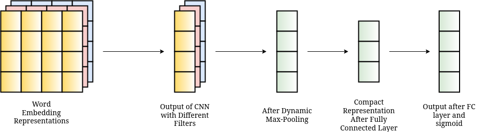
Finally, the output of the bottleneck layer is passed through another fully connected layer with output size . The binary cross entropy loss is observed to work the best used for this method.
The ablation studies performed in the paper show that BCE loss, bottleneck layer, and dynamic max pooling each contribute to the improvement of the model. Though XML-CNN was slower than the tree based methods, it clearly outperformed them in terms of performance. It also performed better than linear algebra based methods, showing the potential deep learning held for the XML field.
However, XML-CNN was unable to capture the most relevant parts of the input text to each label, because the same text representation is given for all the labels. Sequence to Sequence based methods like MLC2Seq Nam et al. (2017) were also not suited for the task since the underlying assumption that labels are predicted sequentially is not reasonable in extreme classification. You et al. (2019) proposed AttentionXML, which used a BiLSTM (bidirectional long short-term memory) to capture long-distance dependency among words and a multi-label attention to capture the most relevant parts of texts for each label. Since application of attention to train on each label with the full dataset is not possible for large datasets, there must be a method for training on only the most relevant samples for each label. For this, AttentionXML uses a shallow and wide Probabilistic Label Tree (PLT) built on the labels.
The first step is to create the PLT, which is be done by hierarchical clustering algorithm followed by a compression algorithm to reduce depth. This step is similar to that of Parabel Prabhu et al. (2018) where we create a label tree, but here the tree is constructed to be wide and shallow. In effect, the label tree resembles that of Bonsai Khandagale et al. (2020). The reason for creation of a wide tree instead of a deep one is to prevent error propagation through the levels. The leaves correspond to an original label while the internal nodes correspond to meta or pseudo labels. Each node predicts , ie the probability that label or pseudo-label is present, given that parent of is present. Thus, the marginal probability for each label being present is given by the product of probabilities in its path in the PLT i.e.,
The value of the marginal probabilities is predicted by the attention based deep learning network. As depicted in 10, the architecture consists of a bidirectional LSTM which finds embeddings for the words and then followed by a 2-layer fully connected neural network which finally predicts the probability that the current label is active given the input. There is one block of such network per layer of the PLT.
The input to the fully connected layers is given by using a attention based mechanism which can find if a word embedding is relevant to the label. Finally, the parameters of the fully connected layers are shared among the different labels in each layer, as they perform the same function. This also largely helps reduce model size. Further, to reduce training cost, the model weights of each layer is initialized with the weights of the previous layer.
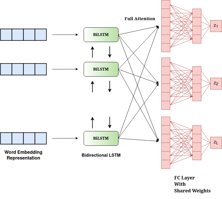
It is to be noted that even if this network is directly used, the training time will be infeasible as each label would have to train on each sample. However, we do not need to train on every sample for a particular label. Hence, only the samples which contain the label and a few more negative samples are used for training.
AttentionXML outperforms XML-CNN and most other methods in terms of P@1 scores. Further, the good PSP scores show that AttentionXML performs well on tail labels as well. The utility of multi-head attention is proven in the ablation study. However, AttentionXML is not easy to train as the training and prediction times are much larger compared to other methods and hence does not scale well to larger datasets.
Despite the usage of attention by AttentionXML, a direct attempt at using the pretrained transformers for XML was not yet made. The transfer learning of pretrained transformers for this task could be the solution to the large training times required by AttentionXML. Chang et al. (2020) made the first attempt at using pretrained transformers for the XML task in the model XTransformer. Transformers like BERT Devlin et al. (2018), RoBERTa Liu et al. (2019), and XLNet Yang et al. (2019) are highly successful in the NLP domain where they outperformed most other methods on tasks like question answering, POS tagging, and sentence classification due to their ability to generate contextual embeddings for words and sentences which are applicable to downstream tasks. However, application of these models for the XML problem was not so straightforward even though XML is primarily a text classification problem.
The difficulty was because of the large number of labels and the output space sparsity. Many of the labels do not have enough samples to be able to be able to train large deep neural networks and hence direct application of pretrained transformers led to bad results and memory issues. Xtransformer handles this by reducing the larger problem into smaller subproblems, like in tree based methods, and then training the transformers to predict in this smaller problem. Each of the subproblems are eventually solved to get the final predictions.
More concretely, the XTransformer model consists of three parts or modules. The first module is called Semantic Label Indexing, which is responsible for the division of the larger problem into smaller subproblems. For this, a clustering of the labels is performed, creating clusters where . The clusters are created by finding a label to cluster assignment matrix where if label belongs to cluster . This matrix can be created by using hierarchical clustering algorithms and the clusters are represented based on the mean of transformer embeddings of the label text for the labels present in the cluster.
These clusters are then used as meta-labels for the problem of fine tuning the transformer models in the second module called the Neural Matcher. Since the number of meta-labels is much smaller, the label sparsity issue due to tail labels is avoided. The transformers are trained to map from instances to the relevant clusters. Embeddings are thus trained for each instance .
In the third module after the matching step, a small subset of label clusters is selected for each instance from which we are required to find a relevance score of each label. For performing this final step which is crucial to prediction, a one-vs-all classifier is trained for each label. The instances on which each label trains must be limited in number to allow efficient training. Techniques like picking teacher-forcing negatives (for each label , picking only the instances instances with label or with any of the labels in the same cluster as label ) allow picking only a small subset of “hard” instances.
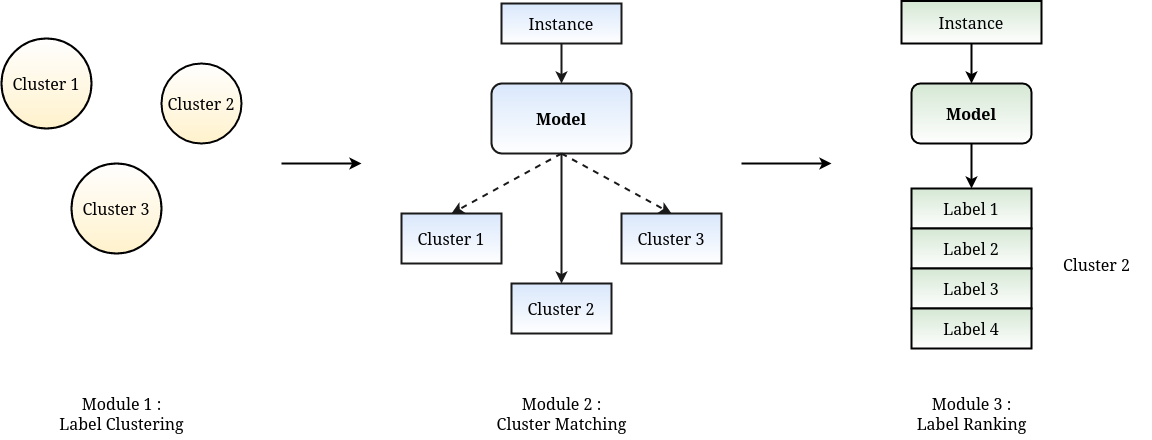
During prediction, a subset of clusters are selected by the Matcher. All the labels selected from each of the clusters are then passed the test instance to which each one-vs-all classifier gives a relevance score to decide if the label is relevant to the instance, based on which the label ranking is done. XTransformer is successfully able to perform well on all datasets and was only outperformed by AttentionXML on some datasets at the time.
Some other successful methods which attempt to fine tune transformers have been recently proposed such as APLC-XLNet, Ye et al. (2020) which uses transfer learning of the popular transformer model XLNet Yang et al. (2019). As with previous methods, performing this directly is not possible, hence this methods uses Adaptive Probabilistic Label Clusters, which attempts a clustering based on separating the head and tail clusters, and then assigning head cluster as the root of a tree and tail clusters as leaves.
Another method which uses transformers to perform extreme classification is LightXML Jiang et al. (2021). This paper points out that methods like AttentionXML and XTransformer suffer from static negative sampling, which highly reduces the ability of the model. The main advantage of LightXML over other methods using static negative sampling is that the model does not overfit to specific negative samples. LightXML performs dynamic negative sampling by using a generator-discriminator like method in which the label recalling is performed by a module (generator) and the label ranking is done by another module. This procedure allows each module to try and improve its own objective while enhancing the other, thus leading to better performance overall.
A general trend can be observed from papers like AttentionXML and XTransformer, where deep learning methods are not directly applied to the problem due to scalability issues. Instead, the deep learning model is applied to a smaller subproblem to obtain intermediate features which can be further used in the problem. Also, negative sampling is generally used for training the final model as training on all samples is not feasible. Dahiya et al. (2021b) comes up with a general framework for applying deep learning methods to XML called DeepXML. Consequently, they propose a new method called ASTEC using the existing method which achieves a new state of the art for some datasets in the domain.
The paper defines DeepXML to be a framework with four modules. Each module is designed to be fairly of low complexity, allowing the entire method to scale to large datasets easily. Not all the methods need to have each of the modules depending on the utility, and the module algorithm can be switched to another algorithm easily without affecting the entire method.
The first module of the framework is for training intermediate representations for the features . Here, should be as close as possible to the final representation of the features which would be the feature representations if the entire problem was optimized directly. Since features cannot be trained on the entire problem, a surrogate label selection procedure is followed to ensure that the problem is tractable. Some examples of surrogate label selection procedures could be label subset selection, label clustering or or label projection into a smaller space.
The second module of DeepXML is the label shortlisting or the negative sampling step, where for each sample, we select the most confusing of the ”hardest” labels. We select for each sample such that and these labels are most likely to be predicted as positive labels for the samples. This negative sampling is done based on the intermediate features learnt in the first module and any method can be used for this procedure such as graphs, trees, clustering or hashing.
The third module is based on transfer learning to obtain the final feature representations from the initial feature representations learnt in the first module. The parameters can be re-trained from the first module, but it must be ensured that the final feature representation should not be too far from the initial representation.
In the fourth module, the final classifier is learnt. This classifier uses the feature representation from the third module and the negative samples from the second module. Since the number of instances for each label is not excessive due to the negative sampling, the model training time is limited. The third and fourth modules can be combined as required.
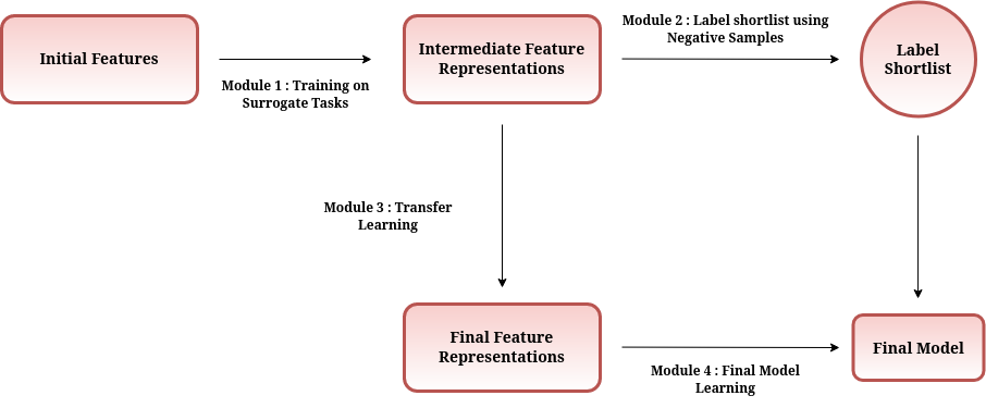
In the paper Dahiya et al. (2021b), the method ASTEC is proposed which uses the DeepXML framework. For the first module, it uses a tree based clustering method to obtain the surrogate labels for training intermediate features. For the second module, an Approximate Nearest Neighbor Search (ANNS) data structure is used for shortlisting. Modules 3 and 4 are trained together where the transfer learning is done by a simple transfer matrix, while the final classifiers are simple one-vs-all classifiers.
More methods using this framework have also been proposed and several existing ones, such as XTransformer can can be formulated to fit into this framework. Mittal et al. (2021a) proposes a method DECAF using this framework which incorporates the label metadata. Mittal et al. (2021b) proposes ECLARE which utilizes label to label correlation as well as label text to give a new method following the DeepXML framework. GalaXC Saini et al. (2021) is another method in this framework which uses graph neural networks on the combined document label space.
Recent advances have been made in the field by using the label features in addition to the instance features. Since in many of the XML datasets, the labels are also entities with some text information. This allows using the label text for learning better models. Different methods try to utilize the label features in different ways. For example, DECAF Mittal et al. (2021a) directly incorporates label text into the classification procedure by embedding the instances and labels separately and then using a ranker to predict which label embedding is most relevant to the instance.
On the other hand, GalaXC Saini et al. (2021) utilizes graph neural networks to learn embeddings jointly over documents and labels. The method uses convolutions of varying size to develop an attention mechanism for learning several representations for each node, where each document and label is a node. Multiple hops over the joint label and document graph allow collection of information over related labels, other documents with these labels and so on. This is used for shortlisting and then prediction is finally made by using the label attention mechanism. ECLARE Mittal et al. (2021b) also uses a similar method by accommodating for label metadata and label correlations.
SiameseXML Dahiya et al. (2021a) also uses label features, but it aims to learn joint embeddings for the labels and features by using the concept of Siamese Networks Chen et al. (2020), Schroff et al. (2015) where a triplet or contrastive loss is used with a hard negative mining procedure. The main goal is to learn common embeddings for instances and labels where instances are close to the respective positive labels and far from the other negative labels. This concept is adapted to the extreme classification scenario by using the DeepXML framework.
The paper Dahiya et al. (2022) suggests another method NGAME which uses Siamese Networks for extreme classification. A common method of using Siamese Networks is using minibatches. The set of candidate labels contains all the labels which appear in at least one of the other instances in the minibatch. The minibatch size, if constructed independently, cannot be too large as the set of labels would be to big. This leads to slower training. NGAME strategically constructs the mini-batches such that the samples are close, thus leading to informative negative samples as compared to random samples. This leads to better convergence and faster training.
Comparison between methods
-
•
XML-CNN although the first of the deep learning methods in XML, is no longer a competitive method in terms of performance. This is mainly because CNN’s are not the best at capturing the information from text, and hence have been outperformed by most other methods.
-
•
AttentionXML and XTransformer are both methods which require a lot of training time. However, they still remain relevant due to the fact that they perform significantly well on some datasets. In particular, AttentionXML performs well on datasets with high average feature text length.
-
•
DeepXML based methods such as SiameseXML, ECLARE and NGAME are currently among the best performing methods in XML.
Over the last five years, deep learning based methods have outperformed all other methods in terms of performance. They have much higher accuracies than tree based methods, but can be slower in terms of train and test complexities and have higher model sizes.
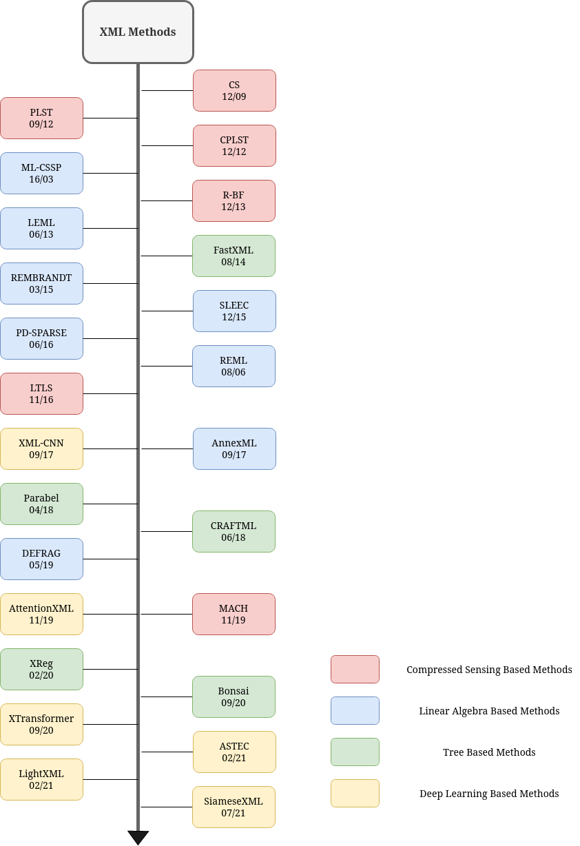
5 Applications of Extreme Classification
Extreme Classification has several applications, especially in cases where the data is too large to be processed manually or semi-manually.
5.0.1 Document Tagging
XML is highly useful for tagging documents with labels which can be selected multiple at a time. The features can be formulated as some representation of the document, while labels are the possible tags.
For example, tagging of Wikipedia articles with relevant labels is a problem which is suited for XML due to the fact that there are a very large number of labels, some of which are very specific to the articles. This leads to a large tail label distribution which is typical in XML problems.
5.0.2 Product Recommendation
Given a keyword or a “search phrase”, the problem of determining which products to show given the product description and other information can also be converted to an extreme classification problem. The “search phrase” or the query can be treated as a feature while the different products act as labels. Amazon has several product recommendation datasets such as Amazon-670K, AmazonCat-13K and AmazonTitles-3M with large label spaces which serve as benchmarking datasets in XML Medini et al. (2019).
5.0.3 Advertising
Finding the appropriate advertisements from the bid phrases given in an advertisement using the user search phrase is also a popular application of XML. Search engines such as Bing have adopted XML to highly improve their click-through rates Dahiya et al. (2021b). Al alternate probelem in advertizing, which is showing personalized ads using the search history of the user can also be modelled as an XML problem, with the user search history being included in the features and the advertisements as labels.
5.1 Multimodal Extreme Classification
Recently, there has been work in extending extreme classification methods to non text domains. Mittal et al. (2022) has recently proposed a new product recommendation dataset MM-AmazonTitles-300K created from Amazon listings of products, each accompanied by an image and text. The paper also suggests a modularized method called MUFIN, which aims to find recommendations based on search query taking into account both images and text. The method creates simultaneous data point and label embeddings (by combining the image and text embeddings) and then uses DeepXML like modules to train the final model.
Acknowledgments
We would like to acknowledge support of MAPG grant, Qualcomm grant, etc.
Appendix A.
References
- Babbar and Schölkopf (2016) Rohit Babbar and Bernhard Schölkopf. Dismec: Distributed sparse machines for extreme multi-label classification. In WSDM ’17, 2016.
- Balasubramanian and Lebanon (2012) Krishnakumar Balasubramanian and Guy Lebanon. The landmark selection method for multiple output prediction. In Proceedings of the 29th International Coference on International Conference on Machine Learning, ICML’12, page 283–290, Madison, WI, USA, 2012. Omnipress. ISBN 9781450312851.
- Bhatia et al. (2016) K. Bhatia, K. Dahiya, H. Jain, P. Kar, A. Mittal, Y. Prabhu, and M. Varma. The extreme classification repository: Multi-label datasets and code, 2016. URL http://manikvarma.org/downloads/XC/XMLRepository.html.
- Bhatia et al. (2015) Kush Bhatia, Himanshu Jain, Purushottam Kar, Manik Varma, and Prateek Jain. Sparse local embeddings for extreme multi-label classification. In C. Cortes, N. D. Lawrence, D. D. Lee, M. Sugiyama, and R. Garnett, editors, Advances in Neural Information Processing Systems 28, pages 730–738. Curran Associates, Inc., 2015.
- Bi and Kwok (2013) Wei Bi and James T. Kwok. Efficient multi-label classification with many labels. In Proceedings of the 30th International Conference on International Conference on Machine Learning - Volume 28, ICML’13, page III–405–III–413. JMLR.org, 2013.
- Blondel et al. (2008) Vincent D Blondel, Jean-Loup Guillaume, Renaud Lambiotte, and Etienne Lefebvre. Fast unfolding of communities in large networks. Journal of Statistical Mechanics: Theory and Experiment, 2008(10):P10008, oct 2008. doi: 10.1088/1742-5468/2008/10/p10008.
- Bloom (1970) Burton H. Bloom. Space/time trade-offs in hash coding with allowable errors. Commun. ACM, 13(7):422–426, July 1970. ISSN 0001-0782. doi: 10.1145/362686.362692.
- Boutsidis et al. (2009) Christos Boutsidis, Michael W. Mahoney, and Petros Drineas. An improved approximation algorithm for the column subset selection problem. In Proceedings of the Twentieth Annual ACM-SIAM Symposium on Discrete Algorithms, SODA ’09, page 968–977, USA, 2009. Society for Industrial and Applied Mathematics.
- Chang et al. (2020) Wei-Cheng Chang, Hsiang-Fu Yu, Kai Zhong, Yiming Yang, and Inderjit S Dhillon. Taming pretrained transformers for extreme multi-label text classification. In Proceedings of the 26th ACM SIGKDD International Conference on Knowledge Discovery & Data Mining, pages 3163–3171, 2020.
- Charikar et al. (2002) Moses Charikar, Kevin Chen, and Martin Farach-Colton. Finding frequent items in data streams. In Proceedings of the 29th International Colloquium on Automata, Languages and Programming, ICALP ’02, page 693–703, Berlin, Heidelberg, 2002. Springer-Verlag. ISBN 3540438645.
- Chen et al. (2020) Ting Chen, Simon Kornblith, Mohammad Norouzi, and Geoffrey Hinton. A simple framework for contrastive learning of visual representations. In International conference on machine learning, pages 1597–1607. PMLR, 2020.
- Chen (2015) Yahui Chen. Convolutional neural network for sentence classification. Master’s thesis, University of Waterloo, 2015.
- Cissé et al. (2013) Moustapha Cissé, Nicolas Usunier, Thierry Artieres, and Patrick Gallinari. Robust bloom filters for large multilabel classification tasks. In Proceedings of the 26th International Conference on Neural Information Processing Systems - Volume 2, NIPS’13, page 1851–1859, Red Hook, NY, USA, 2013. Curran Associates Inc.
- Dahiya et al. (2021a) Kunal Dahiya, Ananye Agarwal, Deepak Saini, K Gururaj, Jian Jiao, Amit Singh, Sumeet Agarwal, Purushottam Kar, and Manik Varma. Siamesexml: Siamese networks meet extreme classifiers with 100m labels. In International Conference on Machine Learning, pages 2330–2340. PMLR, 2021a.
- Dahiya et al. (2021b) Kunal Dahiya, Deepak Saini, Anshul Mittal, Ankush Shaw, Kushal Dave, Akshay Soni, Himanshu Jain, Sumeet Agarwal, and Manik Varma. Deepxml: A deep extreme multi-label learning framework applied to short text documents. In Proceedings of the 14th ACM International Conference on Web Search and Data Mining, pages 31–39, 2021b.
- Dahiya et al. (2022) Kunal Dahiya, Nilesh Gupta, Deepak Saini, Akshay Soni, Yajun Wang, Kushal Dave, Jian Jiao, Prasenjit Dey, Amit Singh, Deepesh Hada, et al. Ngame: Negative mining-aware mini-batching for extreme classification. arXiv preprint arXiv:2207.04452, 2022.
- Devlin et al. (2018) Jacob Devlin, Ming-Wei Chang, Kenton Lee, and Kristina Toutanova. Bert: Pre-training of deep bidirectional transformers for language understanding. arXiv preprint arXiv:1810.04805, 2018.
- Dong et al. (2011) Wei Dong, Charikar Moses, and Kai Li. Efficient k-nearest neighbor graph construction for generic similarity measures. In Proceedings of the 20th International Conference on World Wide Web, WWW ’11, page 577–586, New York, NY, USA, 2011. Association for Computing Machinery. ISBN 9781450306324. doi: 10.1145/1963405.1963487.
- Evron et al. (2018) Itay Evron, Edward Moroshko, and Koby Crammer. Efficient loss-based decoding on graphs for extreme classification. Advances in Neural Information Processing Systems, 31, 2018.
- Friedland and Torokhti (2006) Shmuel Friedland and Anatoli Torokhti. Generalized rank-constrained matrix approximations, 2006.
- Halko et al. (2011) N. Halko, P. G. Martinsson, and J. A. Tropp. Finding structure with randomness: Probabilistic algorithms for constructing approximate matrix decompositions. SIAM Review, 53(2):217–288, 2011. doi: 10.1137/090771806.
- Hsu et al. (2009) Daniel J. Hsu, Sham M. Kakade, John Langford, and Tong Zhang. Multi-label prediction via compressed sensing. CoRR, abs/0902.1284, 2009.
- Jain et al. (2016) Himanshu Jain, Yashoteja Prabhu, and Manik Varma. Extreme multi-label loss functions for recommendation, tagging, ranking & other missing label applications. In Proceedings of the 22nd ACM SIGKDD International Conference on Knowledge Discovery and Data Mining, pages 935–944, 2016.
- Jain et al. (2010) Prateek Jain, Raghu Meka, and Inderjit Dhillon. Guaranteed rank minimization via singular value projection. In Proceedings of the 23rd International Conference on Neural Information Processing Systems - Volume 1, NIPS’10, pages 937–945, USA, 2010. Curran Associates Inc. URL http://dl.acm.org/citation.cfm?id=2997189.2997294.
- Jalan and Kar (2019) Ankit Jalan and Purushottam Kar. Accelerating extreme classification via adaptive feature agglomeration. CoRR, abs/1905.11769, 2019.
- Jasinska and Karampatziakis (2016) Kalina Jasinska and Nikos Karampatziakis. Log-time and log-space extreme classification. arXiv preprint arXiv:1611.01964, 2016.
- Jiang et al. (2021) Ting Jiang, Deqing Wang, Leilei Sun, Huayi Yang, Zhengyang Zhao, and Fuzhen Zhuang. Lightxml: Transformer with dynamic negative sampling for high-performance extreme multi-label text classification. In Proceedings of the AAAI Conference on Artificial Intelligence, volume 35, pages 7987–7994, 2021.
- Joulin et al. (2016) Armand Joulin, Edouard Grave, Piotr Bojanowski, and Tomas Mikolov. Bag of tricks for efficient text classification. arXiv preprint arXiv:1607.01759, 2016.
- Khandagale et al. (2020) Sujay Khandagale, Han Xiao, and Rohit Babbar. Bonsai: diverse and shallow trees for extreme multi-label classification. Machine Learning, 109(11):2099–2119, 2020.
- Lacoste-Julien and Jaggi (2015) Simon Lacoste-Julien and Martin Jaggi. On the global linear convergence of frank-wolfe optimization variants. Advances in neural information processing systems, 28, 2015.
- Lacoste-Julien et al. (2013) Simon Lacoste-Julien, Martin Jaggi, Mark Schmidt, and Patrick Pletscher. Block-coordinate frank-wolfe optimization for structural svms. In International Conference on Machine Learning, pages 53–61. PMLR, 2013.
- Liu et al. (2015) Feng Liu, Xiaofeng Zhang, Yunming Ye, Yahong Zhao, and Yan Li. Mlrf: multi-label classification through random forest with label-set partition. In International conference on intelligent computing, pages 407–418. Springer, 2015.
- Liu et al. (2017) Jingzhou Liu, Wei-Cheng Chang, Yuexin Wu, and Yiming Yang. Deep learning for extreme multi-label text classification. In Proceedings of the 40th international ACM SIGIR conference on research and development in information retrieval, pages 115–124, 2017.
- Liu et al. (2019) Yinhan Liu, Myle Ott, Naman Goyal, Jingfei Du, Mandar Joshi, Danqi Chen, Omer Levy, Mike Lewis, Luke Zettlemoyer, and Veselin Stoyanov. Roberta: A robustly optimized bert pretraining approach. arXiv preprint arXiv:1907.11692, 2019.
- Loza Mencía and Fürnkranz (2008) Eneldo Loza Mencía and Johannes Fürnkranz. Efficient pairwise multilabel classification for large-scale problems in the legal domain. In Joint European Conference on Machine Learning and Knowledge Discovery in Databases, pages 50–65. Springer, 2008.
- McAuley and Leskovec (2013) Julian McAuley and Jure Leskovec. Hidden factors and hidden topics: understanding rating dimensions with review text. In Proceedings of the 7th ACM conference on Recommender systems, pages 165–172, 2013.
- McAuley et al. (2015a) Julian McAuley, Rahul Pandey, and Jure Leskovec. Inferring networks of substitutable and complementary products. In Proceedings of the 21th ACM SIGKDD international conference on knowledge discovery and data mining, pages 785–794, 2015a.
- McAuley et al. (2015b) Julian McAuley, Christopher Targett, Qinfeng Shi, and Anton Van Den Hengel. Image-based recommendations on styles and substitutes. In Proceedings of the 38th international ACM SIGIR conference on research and development in information retrieval, pages 43–52, 2015b.
- Medini et al. (2019) Tharun Kumar Reddy Medini, Qixuan Huang, Yiqiu Wang, Vijai Mohan, and Anshumali Shrivastava. Extreme classification in log memory using count-min sketch: A case study of amazon search with 50m products. In H. Wallach, H. Larochelle, A. Beygelzimer, F. d Alché-Buc, E. Fox, and R. Garnett, editors, Advances in Neural Information Processing Systems 32, pages 13265–13275. Curran Associates, Inc., 2019.
- Mineiro and Karampatziakis (2014) Paul Mineiro and Nikos Karampatziakis. Fast label embeddings for extremely large output spaces. CoRR, abs/1412.6547, 2014. URL http://arxiv.org/abs/1412.6547.
- Mittal et al. (2021a) Anshul Mittal, Kunal Dahiya, Sheshansh Agrawal, Deepak Saini, Sumeet Agarwal, Purushottam Kar, and Manik Varma. Decaf: Deep extreme classification with label features. In Proceedings of the 14th ACM International Conference on Web Search and Data Mining, pages 49–57, 2021a.
- Mittal et al. (2021b) Anshul Mittal, Noveen Sachdeva, Sheshansh Agrawal, Sumeet Agarwal, Purushottam Kar, and Manik Varma. Eclare: Extreme classification with label graph correlations. In Proceedings of the Web Conference 2021, pages 3721–3732, 2021b.
- Mittal et al. (2022) Anshul Mittal, Kunal Dahiya, Shreya Malani, Janani Ramaswamy, Seba Kuruvilla, Jitendra Ajmera, Keng-hao Chang, Sumeet Agarwal, Purushottam Kar, and Manik Varma. Multi-modal extreme classification. In Proceedings of the IEEE/CVF Conference on Computer Vision and Pattern Recognition, pages 12393–12402, 2022.
- Nam et al. (2017) Jinseok Nam, Eneldo Loza Mencía, Hyunwoo J Kim, and Johannes Fürnkranz. Maximizing subset accuracy with recurrent neural networks in multi-label classification. In I. Guyon, U. V. Luxburg, S. Bengio, H. Wallach, R. Fergus, S. Vishwanathan, and R. Garnett, editors, Advances in Neural Information Processing Systems 30, pages 5413–5423. Curran Associates, Inc., 2017.
- nan Chen and tien Lin (2012) Yao nan Chen and Hsuan tien Lin. Feature-aware label space dimension reduction for multi-label classification. In F. Pereira, C. J. C. Burges, L. Bottou, and K. Q. Weinberger, editors, Advances in Neural Information Processing Systems 25, pages 1529–1537. Curran Associates, Inc., 2012.
- Pati et al. (1993) Yagyensh Chandra Pati, Ramin Rezaiifar, and Perinkulam Sambamurthy Krishnaprasad. Orthogonal matching pursuit: Recursive function approximation with applications to wavelet decomposition. In Proceedings of 27th Asilomar conference on signals, systems and computers, pages 40–44. IEEE, 1993.
- Prabhu and Varma (2014) Yashoteja Prabhu and Manik Varma. Fastxml: A fast, accurate and stable tree-classifier for extreme multi-label learning. In Proceedings of the 20th ACM SIGKDD international conference on Knowledge discovery and data mining, pages 263–272, 2014.
- Prabhu et al. (2018) Yashoteja Prabhu, Anil Kag, Shrutendra Harsola, Rahul Agrawal, and Manik Varma. Parabel: Partitioned label trees for extreme classification with application to dynamic search advertising. In Proceedings of the 2018 World Wide Web Conference, pages 993–1002, 2018.
- Prabhu et al. (2020) Yashoteja Prabhu, Aditya Kusupati, Nilesh Gupta, and Manik Varma. Extreme regression for dynamic search advertising. Proceedings of the 13th International Conference on Web Search and Data Mining, Jan 2020. doi: 10.1145/3336191.3371768.
- Saini et al. (2021) Deepak Saini, Arnav Kumar Jain, Kushal Dave, Jian Jiao, Amit Singh, Ruofei Zhang, and Manik Varma. Galaxc: Graph neural networks with labelwise attention for extreme classification. In Proceedings of the Web Conference 2021, pages 3733–3744, 2021.
- Schroff et al. (2015) Florian Schroff, Dmitry Kalenichenko, and James Philbin. Facenet: A unified embedding for face recognition and clustering. In Proceedings of the IEEE conference on computer vision and pattern recognition, pages 815–823, 2015.
- Seshadri and Sundberg (1994) Nambirajan Seshadri and C-EW Sundberg. List viterbi decoding algorithms with applications. IEEE transactions on communications, 42(234):313–323, 1994.
- Siblini et al. (2018) Wissam Siblini, Frank Meyer, and Pascale Kuntz. Craftml, an efficient clustering-based random forest for extreme multi-label learning. In ICML, 2018.
- Sprechmann et al. (2013) Pablo Sprechmann, Roee Litman, Tal Ben Yakar, Alex Bronstein, and Guillermo Sapiro. Efficient supervised sparse analysis and synthesis operators. In Proceedings of the 26th International Conference on Neural Information Processing Systems - Volume 1, NIPS’13, pages 908–916, USA, 2013. Curran Associates Inc.
- Tagami (2017) Yukihiro Tagami. Annexml: Approximate nearest neighbor search for extreme multi-label classification. In Proceedings of the 23rd ACM SIGKDD International Conference on Knowledge Discovery and Data Mining, KDD ’17, pages 455–464, New York, NY, USA, 2017. ACM. ISBN 978-1-4503-4887-4. doi: 10.1145/3097983.3097987. URL http://doi.acm.org/10.1145/3097983.3097987.
- Tai and Lin (2012) Farbound Tai and Hsuan-Tien Lin. Multilabel classification with principal label space transformation. Neural Comput., 24(9):2508–2542, September 2012. ISSN 0899-7667. doi: 10.1162/NECO-a-00320.
- Weston et al. (2013) Jason Weston, Ameesh Makadia, and Hector Yee. Label partitioning for sublinear ranking. In International conference on machine learning, pages 181–189. PMLR, 2013.
- Xu et al. (2016) Chang Xu, Dacheng Tao, and Chao Xu. Robust extreme multi-label learning. In Proceedings of the 22nd ACM SIGKDD International Conference on Knowledge Discovery and Data Mining, KDD ’16, page 1275–1284, New York, NY, USA, 2016. Association for Computing Machinery. ISBN 9781450342322. doi: 10.1145/2939672.2939798.
- Yang et al. (2019) Zhilin Yang, Zihang Dai, Yiming Yang, Jaime Carbonell, Russ R Salakhutdinov, and Quoc V Le. Xlnet: Generalized autoregressive pretraining for language understanding. Advances in neural information processing systems, 32, 2019.
- Ye et al. (2020) Hui Ye, Zhiyu Chen, Da-Han Wang, and Brian Davison. Pretrained generalized autoregressive model with adaptive probabilistic label clusters for extreme multi-label text classification. In International Conference on Machine Learning, pages 10809–10819. PMLR, 2020.
- Yen et al. (2017) Ian E.H. Yen, Xiangru Huang, Wei Dai, Pradeep Ravikumar, Inderjit Dhillon, and Eric Xing. Ppdsparse: A parallel primal-dual sparse method for extreme classification. In Proceedings of the 23rd ACM SIGKDD International Conference on Knowledge Discovery and Data Mining, KDD ’17, page 545–553, New York, NY, USA, 2017. Association for Computing Machinery. ISBN 9781450348874. doi: 10.1145/3097983.3098083.
- Yen et al. (2016) Ian En-Hsu Yen, Xiangru Huang, Pradeep Ravikumar, Kai Zhong, and Inderjit S. Dhillon. Pd-sparse : A primal and dual sparse approach to extreme multiclass and multilabel classification. In ICML, 2016.
- Yih et al. (2011) Wen-tau Yih, Kristina Toutanova, John C. Platt, and Christopher Meek. Learning discriminative projections for text similarity measures. In Proceedings of the Fifteenth Conference on Computational Natural Language Learning, pages 247–256, Portland, Oregon, USA, June 2011. Association for Computational Linguistics.
- You et al. (2019) Ronghui You, Zihan Zhang, Ziye Wang, Suyang Dai, Hiroshi Mamitsuka, and Shanfeng Zhu. Attentionxml: Label tree-based attention-aware deep model for high-performance extreme multi-label text classification. Advances in Neural Information Processing Systems, 32, 2019.
- Yu et al. (2013) Hsiang-Fu Yu, Prateek Jain, and Inderjit S. Dhillon. Large-scale multi-label learning with missing labels. CoRR, abs/1307.5101, 2013.
- Zubiaga (2012) Arkaitz Zubiaga. Enhancing navigation on wikipedia with social tags. arXiv preprint arXiv:1202.5469, 2012.