Reconstruction techniques for quantum trees

Abstract

The inverse problem of recovery of a potential on a quantum tree graph from Weyl’s matrix given at a number of points is considered. A method for its numerical solution is proposed. The overall approach is based on the leaf peeling method combined with Neumann series of Bessel functions (NSBF) representations for solutions of Sturm-Liouville equations. In each step, the solution of the arising inverse problems reduces to dealing with the NSBF coefficients.

The leaf peeling method allows one to localize the general inverse problem to local problems on sheaves, while the approach based on the NSBF representations leads to splitting the local problems into two-spectra inverse problems on separate edges and reduce them to systems of linear algebraic equations for the NSBF coefficients. Moreover, the potential on each edge is recovered from the very first NSBF coefficient. The proposed method leads to an efficient numerical algorithm that is illustrated by numerical tests.

1 Introduction

Quantum graphs and in particular inverse problems on quantum graphs find numerous applications in science and engineering and give rise to challenging problems involving many areas of modern mathematics, from combinatorics to partial differential equations and spectral theory. A number of surveys and collections of papers on quantum graphs appeared last years, including the first books on this topic by Berkolaiko and Kuchment [13] and Mugnolo [29]. Theory of inverse problems on quantum graphs is an actively developing research area of applied mathematics, providing existence and uniqueness results and possible approaches for solution (see, e.g., [25, 35, 12, 8, 9, 4]).

To date, there are few papers presenting methods apt for numerical solution of inverse problems on quantum graphs [12, 3, 7, 6]. Since the problems of space discretization of differential equations on metric graphs turn out to be very difficult, and even the forward boundary value problems on graphs present considerable numerical challenges (see, e.g. [2]), a promising path for efficient solution of inverse problems seems to go through and involve analytical representations of solutions. In [7, 6] such approach was developed for star shaped graphs. It is based on the use of very special functional series representations for solutions of the Sturm-Liouville equation

$$-y^{\prime\prime}+q(x)y=\rho^{2}y,\text{\quad}x\in\left(0,L\right),\quad q\in L_{1}\left(0,L\right),\quad\rho\in\mathbb{C}.$$

These representations have the form of so-called Neumann series of Bessel functions (NSBF) (see, e.g., [33, Chapter XVI], [34] and the recent monograph on the subject [11] and references therein) and were obtained in [21] as a result of the expansion of the transmutation operator kernel (see, e.g., [16], [18], [27], [28], [31]) into a Fourier-Legendre series. The NSBF representations possess certain unique features, which make them especially convenient for solving inverse spectral problems. The remainders of the series admit bounds, which are independent of $\operatorname{Re}\rho$. This facilitates dealing with approximate solutions (partial sums of the NSBF) on very large intervals in $\rho$ and with a non-deteriorating accuracy. Moreover, the knowledge of the very first coefficient of the NSBF representation allows one to recover the potential of the Sturm-Liouville equation, that in practice ensures satisfactory numerical results even when a reduced number of terms of the series is considered and consequently a reduced number of linear algebraic equations is solved in each step.

In the present work we extend this approach, based on the NSBF representations, onto an arbitrary quantum tree. This is done by applying the leaf peeling method developed in [8], combined with new ideas regarding the computation of solutions and their derivatives at abscission points. The inverse problem considered here is the approximate recovery of a potential on a quantum tree from a Weyl matrix given at a set of points $\rho=\rho_{k}$, $k=1,\ldots,K$. The Weyl matrix of a quantum graph is in fact its Dirichlet-to-Neumann map. It plays essential role in all aspects of study of quantum graphs, including spectral theory [35] and controllability [8]. The physical meaning of the inverse problem is the recovery of the differential operator from a measured response at a number of frequencies of a system modelled by the quantum graph.

The leaf peeling method allows one to localize the inverse problem on a tree to an inverse problem on a sheaf, which is a star shaped subgraph whose all but one of the edges are leaf (boundary) edges. After the potential on the leaf edges of the sheaf is recovered, they can be removed, and the leaf peeling method allows one to calculate the Weyl matrix for the new smaller tree. This procedure repeated finitely many times gradually exhausts the whole tree, leading in the last step to an inverse problem on a star shaped graph. A method for its solution with the aid of the NSBF representations was proposed in [6], so that in the present paper we develop a method for solving the local inverse problems on sheaves as well as techniques for computing additional auxiliary functions required for applying the leaf peeling method.

In fact, the overall approach consists in reducing the inverse problem on a graph to operations with the NSBF coefficients of solutions on edges. When solving the local problem, in the first step, we compute the NSBF coefficients for a couple of linearly independent solutions on the leaf edges at the end point of each edge, which is associated with the common vertex of the sheaf. This first step allows us to split the problem into separate problems on leaf edges. Second, the obtained NSBF coefficients are used for computing the Dirichlet-Dirichlet and Neumann-Dirichlet eigenvalues of the potential on each leaf edge. The first feature of the NSBF representations mentioned above ensures the possibility to compute hundreds of the eigenvalues with a uniform accuracy. Thus, on each leaf edge of the sheaf we obtain a two spectra inverse Sturm-Liouville problem. Results on the uniqueness and solvability of such problems are well known and can be found, e.g., in [15], [27], [32], [36]. To this problem we apply the method from [19] which again involves the NSBF representations. It provides for computing certain multiplier constants [14] which relate to the Neumann-Dirichlet eigenfunctions associated to the same eigenvalues but normalized at the opposite endpoints of the interval. This leads to a system of linear algebraic equations for the coefficients of their NSBF representations, already for interior points of the interval. Solving the system we find the very first coefficient, from which the potential is recovered. It is worth mentioning that the NSBF representations were first used for solving inverse Sturm-Liouville problems on a finite interval in [17]. Later on, the approach from [17] was improved in [18] and [23], [24]. In those papers the system of linear algebraic equations was obtained with the aid of the Gelfand-Levitan integral equation. In [19] another approach, based on the consideration of the eigenfunctions normalized at the opposite endpoints, was developed, and this idea was used in [7], [20], [6] and is used in the present work when solving the two-spectra inverse problems on the edges.

Thus, the main result of this work is an efficient method for solving the inverse problem on a quantum tree, consisting in the recovery of a potential from a Weyl matrix. We discuss the numerical implementation of the method and give numerical examples.

In Section 2 we recall the definition of the Weyl matrix and formulate the inverse problem. In Section 3 we write the Weyl solutions in terms of the fundamental systems of solutions on each edge and recall the NSBF representations for solutions of the Sturm-Liouville equation as well as some of their relevant features. In Section 4 we explain in detail the leaf peeling method. In Section 5 we give a detailed description of the proposed method for the solution of the local inverse problem. In Section 6 we summarize the overall method for solving the inverse problem on a tree. In Section 7 we discuss the numerical implementation of the method and numerical examples. Finally, Section 8 contains some concluding remarks.

2 Problem setting

Let $\Omega$ be a finite connected compact graph without cycles (a tree graph) consisting of $P$ edges $e_{1}$,…,$e_{P}$ and $P+1$ vertices $V=\left\{v_{1},...,v_{P+1}\right\}$. The notation $e_{j}\sim v$ means that the edge $e_{j}$ is incident to the vertex $v$. Every edge $e_{j}$ is identified with an interval $(0,L_{j})$ of the real line. The boundary $\Gamma=\left\{\gamma_{1},\ldots,\gamma_{m}\right\}$ of $\Omega$ is the set of all leaves of the graph (the external vertices). The edge adjacent to some $\gamma_{j}\$is called a leaf or boundary edge.

Let $q\in L_{2}(\Omega)$ be real valued, and $\lambda$ a complex number. A continuous function $u$ defined on the graph $\Omega$ is a $P$-tuple of functions $u_{j}\in C\left[0,L_{j}\right]$ satisfying the continuity condition at the internal vertices $v$: $u_{i}(v)=u_{j}(v)$ for all $e_{i},e_{j}\sim v$. Then $u\in C(\Omega)$.

We say that a function $u$ is a solution of the equation

$$-u^{\prime\prime}(x)+q(x)u(x)=\lambda u(x)$$ (2.1)

on the graph $\Omega$ if besides (2.1) the following conditions are satisfied

$$u\in C(\Omega)$$ (2.2)

and

$$\sum_{e_{j}\sim v}\partial u_{j}(v)=0,\text{\quad for all }v\in V\setminus\Gamma.$$ (2.3)

Here $\partial u_{j}(v)$ stands for the derivative of $u$ at the vertex $v$ taken along the edge $e_{j}$ in the direction outward the vertex. The sum in (2.3) is taken over all the edges incident to the internal vertex $v$. Condition (2.3) is known as the Kirchhoff-Neumann condition.

Consider a solution $w_{i}$ of (2.1) such that $w_{i}$ equals zero at all leaves but one: $\gamma_{i}$, at which it equals one. That is $w_{i}$ is a solution of (2.1) such that

$$w_{i}(\gamma_{i})=1\quad\text{and}\quad w_{i}(\gamma_{j})=0\text{ for all }j\neq i.$$

Such a solution $w_{i}$ is called the Weyl solution associated with the leaf $\gamma_{i}$. Since the Dirichlet spectrum of (2.1) is real, the Weyl solution for any $\gamma_{i}$ exists and is unique for all $\lambda\notin\mathbb{R}$.

Definition 2.1

The $m\times m$ matrix-function $\mathbf{M}(\lambda)$, $\lambda\notin\mathbb{R}$, consisting of the elements $\mathbf{M}_{ij}(\lambda)=\partial w_{i}(\gamma_{j})$, $i,j=1,\ldots,m$ is called the Weyl matrix.

In fact, for a fixed value of $\lambda$, the Weyl matrix represents a Dirichlet-to-Neumann map of the quantum graph defined by $\Omega$ and $q\in L_{2}(\Omega)$. Indeed, if $u$ is a solution of (2.1) satisfying the Dirichlet condition at the boundary vertices $u(\gamma,\lambda)=f(\lambda)$, then $\partial u(\gamma,\lambda)=\mathbf{M}(\lambda)f(\lambda)$, $\lambda\notin\mathbb{R}$.

The problem we consider in the present paper can be formulated as follows.

Problem 2.2

Given $\Omega$ and the Weyl matrix at a finite number of points $\lambda_{k}$, $k=1,\ldots,K$, find the potential $q(x)$ approximately.

When the Weyl matrix or even its main diagonal is known everywhere, the potential $q(x)$ is determined uniquely (see, e.g., [35]). The knowledge of the Weyl matrix at a finite number of points may allow one to recover the potential $q(x)$ only approximately.

Practical importance of this inverse problem is quite obvious. The entries of the Weyl matrix represent the response of the physical system described by the quantum graph to a unitary impulse applied at one end while isolating the others. From the knowledge of this response at some values $\lambda_{k}$, $k=1,\ldots,K$ we recover approximately the Sturm-Liouville equation (2.1) on the whole tree graph.

3 Fundamental system of solutions and the Weyl solutions

By $\varphi_{i}(\rho,x)$ and $S_{i}(\rho,x)$ we denote the solutions of the equation

$$-y^{\prime\prime}(x)+q_{i}(x)y(x)=\rho^{2}y(x),\quad x\in(0,L_{i})$$ (3.1)

satisfying the initial conditions

$$\varphi_{i}(\rho,0)=1,\quad\varphi_{i}^{\prime}(\rho,0)=0,$$

$$S_{i}(\rho,0)=0,\quad S_{i}^{\prime}(\rho,0)=1.$$

Here $q_{i}(x)$ is the component of the potential $q(x)$ on the edge $e_{i}$, and $\rho=\sqrt{\lambda}$, $\operatorname{Im}\rho\geq 0$. For a leaf edge $e_{i}$ it is convenient to identify its leaf $\gamma_{i}$ with zero. Then the Weyl solution $w_{i}(\rho,x)$ has the form

$$w_{i}(\rho,x)=\varphi_{i}(\rho,x)+\mathbf{M}_{ii}(\rho^{2})S_{i}(\rho,x)\quad\text{on the adjacent edge }e_{i}$$

and

$$w_{i}(\rho,x)=\mathbf{M}_{ij}(\rho^{2})S_{j}(\rho,x)\quad\text{on every leaf edge }e_{j},\quad j\neq i.$$

On internal edges $e_{j}$ we have

$$w_{i}(\rho,x)=a_{ij}(\rho)\varphi_{j}(\rho,x)+b_{ij}(\rho)S_{j}(\rho,x),$$

where the choice of which vertex lies at zero is arbitrary, and in general the factors $a_{ij}(\rho)$, $b_{ij}(\rho)$ are unknown.

Theorem 3.1 ([21])

The solutions $\varphi_{i}(\rho,x)$ and $S_{i}(\rho,x)$ of (3.1) and their derivatives with respect to $x$ admit the following series representations

$$\varphi_{i}(\rho,x) =\cos\left(\rho x\right)+\sum_{n=0}^{\infty}(-1)^{n}g_{i,n}(x)\mathbf{j}_{2n}(\rho x),$$ (3.2)

$$S_{i}(\rho,x) =\frac{\sin\left(\rho x\right)}{\rho}+\frac{1}{\rho}\sum_{n=0}^{\infty}(-1)^{n}s_{i,n}(x)\mathbf{j}_{2n+1}(\rho x),$$ (3.3)

$$\varphi_{i}^{\prime}(\rho,x) =-\rho\sin\left(\rho x\right)+\frac{\cos\left(\rho x\right)}{2}\int_{0}^{x}q_{i}(t)\,dt+\sum_{n=0}^{\infty}(-1)^{n}\gamma_{i,n}(x)\mathbf{j}_{2n}(\rho x),$$ (3.4)

$$S_{i}^{\prime}(\rho,x) =\cos\left(\rho x\right)+\frac{\sin\left(\rho x\right)}{2\rho}\int_{0}^{x}q_{i}(t)\,dt+\frac{1}{\rho}\sum_{n=0}^{\infty}(-1)^{n}\sigma_{i,n}(x)\mathbf{j}_{2n+1}(\rho x),$$ (3.5)

where $\mathbf{j}_{k}(z)$ stands for the spherical Bessel function of order $k$, $\mathbf{j}_{k}(z):=\sqrt{\frac{\pi}{2z}}J_{k+\frac{1}{2}}(z)$ (see, e.g., [1]). The coefficients $g_{i,n}(x)$, $s_{i,n}(x)$, $\gamma_{i,n}(x)$ and $\sigma_{i,n}(x)$ can be calculated following a simple recurrent integration procedure (see [21] or [18, Sect. 9.4]), starting with

$$g_{i,0}(x) =\varphi_{i}(0,x)-1,\quad s_{i,0}(x)=3\left(\frac{S_{i}(0,x)}{x}-1\right),$$ (3.6)

$$\gamma_{i,0}(x) =g_{i,0}^{\prime}(x)-\frac{1}{2}\int_{0}^{x}q_{i}(t)\,dt,\quad\sigma_{i,0}(x)=\frac{s_{i,0}(x)}{x}+s_{i,0}^{\prime}(x)-\frac{3}{2}\int_{0}^{x}q_{i}(t)\,dt.$$

For every $\rho\in\mathbb{C}$ all the series converge pointwise. For every $x\in\left[0,L_{i}\right]$ the series converge uniformly on any compact set of the complex plane of the variable $\rho$, and the remainders of their partial sums admit estimates independent of $\operatorname{Re}\rho$. In particular, for the partial sums

$$\varphi_{i,N}(\rho,x):=\cos\left(\rho x\right)+\sum_{n=0}^{N}(-1)^{n}g_{i,n}(x)\mathbf{j}_{2n}(\rho x)$$

and

$$S_{i,N}(\rho,x):=\frac{\sin\left(\rho x\right)}{\rho}+\frac{1}{\rho}\sum_{n=0}^{N}(-1)^{n}s_{i,n}(x)\mathbf{j}_{2n+1}(\rho x)$$

we have the estimates

$$\left|\varphi_{i}(\rho,x)-\varphi_{i,N}(\rho,x)\right|\leq\frac{2\varepsilon_{i,N}(x)\,\sinh(Cx)}{C}\quad\text{and}\quad\left|S_{i}(\rho,x)-S_{i,N}(\rho,x)\right|\leq\frac{2\varepsilon_{i,N}(x)\,\sinh(Cx)}{C}$$ (3.7)

for any $\rho\in\mathbb{C}$ belonging to the strip $\left|\operatorname{Im}\rho\right|\leq C$, $C\geq 0$, where $\varepsilon_{i,N}(x)$ is a positive function tending to zero as $N\rightarrow\infty$. Analogous estimates are valid for the derivatives.

Roughly speaking, the approximate solutions and their derivatives approximate the exact ones equally well for small and for large values of $\operatorname{Re}\rho$. This is especially convenient when considering direct and inverse spectral problems that requires operating on a large range of the parameter $\rho$. This unique feature of the series representations (3.2)-(3.5) is due to the fact that they originate from an exact Fourier-Legendre series representation of the integral kernel of the transmutation operator [21], [18, Sect. 9.4] (for the theory of transmutation operators we refer to [27], [28], [31], [36]).

Moreover, the following statement is valid.

Theorem 3.2

For any $\varepsilon>0$ there exists such $N\in\mathbb{N}$ that all zeros of the functions $S_{i}(\rho,L_{i})$ and $\varphi_{i}(\rho,L_{i})$ are approximated by corresponding zeros of the functions $S_{i,N}(\rho,L_{i})$ and $\varphi_{i,N}(\rho,L_{i})$, respectively, with errors uniformly bounded by $\varepsilon$. Moreover, $S_{i,N}(\rho,L_{i})$ and $\varphi_{i,N}(\rho,L_{i})$, have no other zeros.

The proof of this statement is completely analogous to the proof of Proposition 7.1 in [22] and consists in using (3.7), properties of characteristic functions of regular Sturm-Liouville problems and the Rouché theorem.

Series of the type

$$\sum_{n=0}^{\infty}a_{n}J_{\nu+n}(z)$$

are called Neumann series of Bessel functions (NSBF).

Note that formulas (3.6) indicate that the potential $q_{i}(x)$ can be recovered from the first coefficients of the series (3.2) or (3.3). Indeed, we have

$$q_{i}(x)=\frac{g_{i,0}^{\prime\prime}(x)}{g_{i,0}(x)+1}$$ (3.8)

and

$$q_{i}(x)=\frac{\left(xs_{i,0}(x)\right)^{\prime\prime}}{xs_{i,0}(x)+3x}.$$ (3.9)

4 Leaf peeling

The overall strategy is based on the leaf peeling method (developed in [8]) combined with the use of the NSBF representations from Section 3.

Definition 4.1

A star shaped subgraph of a tree graph is called a sheaf if all but one of its edges are leaf edges. The only internal vertex of the sheaf is called the abscission vertex. The only edge which is not a leaf edge is called the stem edge of the sheaf.

In Fig. 1 an example of a tree graph with exactly two sheaves $S_{1}$ and $S_{2}$ is shown. Here $v_{0}$ is the abscission vertex and $e_{0}$ is the stem edge of $S_{1}$.

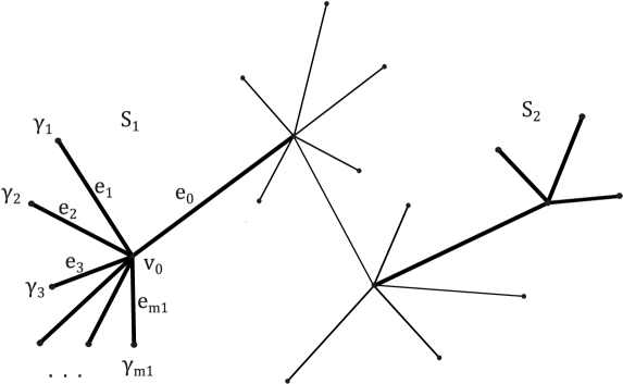
Figure 1: An example of a tree graph with two sheaves $S_{1}$ and $S_{2}$ highlighted in bold lines. Here $v_{0}$ is the abscission vertex and $e_{0}$ is the stem edge of $S_{1}$.

A tree graph, which is not a star shaped graph, contains at least one sheaf [5], [10]. The method developed in [6] allows one to recover the potential on all leaf edges of a sheaf from several entries of the Weyl matrix that correspond to the leaf edges. After that, the leaf peeling method serves for calculating the Weyl matrix for the new (smaller) tree graph obtained by cutting off the leaf edges of the sheaf, so that the abscission vertex becomes a new leaf.

Repeating this leaf peeling procedure one comes eventually to an inverse problem of recovering the potential of a star shaped graph from its Weyl matrix. For this problem the method based on the NSBF representations was developed in [6]. First of all, let us explain the leaf peeling method in more detail.

Consider a tree graph $\Omega$, and assume $S_{1}$ to be its sheaf with an abscission vertex $v_{0}$ and a stem edge $e_{0}$. Without loss of generality we assume that $\gamma_{1},\ldots,\gamma_{m_{1}}$ are the leaves belonging to $S_{1}$. By $\widetilde{\Omega}$ we denote the subgraph $\widetilde{\Omega}=\Omega\setminus\left\{e_{1},\ldots,e_{m_{1}}\right\}$, which is obtained by removing the leaf edges of $S_{1}$ from $\Omega$, so that the vertex $v_{0}$ is a leaf of $\widetilde{\Omega}$, and $e_{0}$ is the corresponding leaf edge. We write $\gamma_{0}=v_{0}$. By $\widetilde{\mathbf{M}}$ we denote the Weyl matrix of $\widetilde{\Omega}$.

Assume that the potential $q(x)$ is already known on each leaf edge $e_{1},\ldots,e_{m_{1}}$ of the sheaf $S_{1}$, so that $q_{1}(x),\ldots,q_{m_{1}}(x)$ are known as well as

$$\varphi_{i}(\rho,L_{i}),\,S_{i}(\rho,L_{i}),\,\varphi_{i}^{\prime}(\rho,L_{i}),\,S_{i}^{\prime}(\rho,L_{i})\quad\text{for\thinspace}1\leq i\leq m_{1}.$$ (4.1)

The problem which is solved by the leaf peeling method consists in computing $\widetilde{\mathbf{M}}$ from $\mathbf{M}$ and (4.1).

We begin with the element $\widetilde{\mathbf{M}}_{00}(\rho^{2})$, which is the derivative at $\gamma_{0}$ of the Weyl solution $\widetilde{w}_{0}(\rho,x)$ on $\widetilde{\Omega}$, which equals one at $\gamma_{0}$ and zero at all other leaves of $\widetilde{\Omega}$, that is, at $\gamma_{j}$ for $j=m_{1}+1,\ldots,m$. Note that

$$\widetilde{w}_{0}(\rho,x)=\frac{w_{1}(\rho,x)}{w_{11}(\rho,\gamma_{0})}\quad\text{on }\widetilde{\Omega}.$$

Hereafter, the notation $w_{ij}(\rho,x)$ means that we consider $j$-th component of a solution $w_{i}(\rho,x)$, that is, the solution $w_{i}(\rho,x)$ on the edge $e_{j}$. Thus,

$$\widetilde{\mathbf{M}}_{00}(\rho^{2})=\frac{\partial w_{10}(\rho,\gamma_{0})}{w_{11}(\rho,\gamma_{0})}=-\sum_{j=1}^{m_{1}}\frac{\partial w_{1j}(\rho,\gamma_{0})}{w_{11}(\rho,\gamma_{0})},$$

where $w_{10}(\rho,x)$ is a component of $w_{1}(\rho,x)$ on $e_{0}$. This can be written in the form

$$\widetilde{\mathbf{M}}_{00}(\rho^{2})=$$

$$-\frac{1}{\varphi_{1}(\rho,L_{1})+\mathbf{M}_{11}(\rho^{2})S_{1}(\rho,L_{1})}\left(\varphi_{1}^{\prime}(\rho,L_{1})+\mathbf{M}_{11}(\rho^{2})S_{1}^{\prime}(\rho,L_{1})+\sum_{j=2}^{m_{1}}\mathbf{M}_{1j}(\rho^{2})S_{j}^{\prime}(\rho,L_{j})\right).$$

Next, it is immediate to see that

$$\widetilde{\mathbf{M}}_{0i}(\rho^{2})=\partial\widetilde{w}_{0}(\rho,\gamma_{i})=\frac{\partial w_{1i}(\rho,\gamma_{i})}{w_{11}(\rho,\gamma_{0})}=\frac{\mathbf{M}_{1i}(\rho^{2})}{w_{11}(\rho,\gamma_{0})}=\frac{\mathbf{M}_{1i}(\rho^{2})}{\varphi_{1}(\rho,L_{1})+\mathbf{M}_{11}(\rho^{2})S_{1}(\rho,L_{1})}$$

for $i=m_{1}+1,\ldots,m$. Thus, we obtained the first row of the Weyl matrix $\widetilde{\mathbf{M}}(\rho^{2})$.

Now choose $i\in\left\{m_{1}+1,\ldots,m\right\}$ and consider the following solution on $\Omega$:

$$u(\rho,x):=w_{i}(\rho,x)-\alpha w_{1}(\rho,x)$$

where $\alpha$ is a constant to be defined. Note that

$$u(\rho,\gamma_{i})=1$$

and

$$u(\rho,\gamma_{j})=0\quad\text{for\thinspace}j=m_{1}+1,\ldots,m\text{ and }j\neq i.$$

Moreover, $\alpha$ can be chosen such that additionally $u(\rho,\gamma_{0})=0$. Indeed, take

$$\alpha=\frac{w_{i}(\rho,\gamma_{0})}{w_{1}(\rho,\gamma_{0})}.$$

Then

$$u(\rho,\gamma_{0})=w_{i}(\rho,\gamma_{0})-\frac{w_{i}(\rho,\gamma_{0})}{w_{1}(\rho,\gamma_{0})}w_{1}(\rho,\gamma_{0})=0$$

and hence with this choice of $\alpha$ we have that

$$\widetilde{w}_{i}(\rho,x)=u(\rho,x)=w_{i}(\rho,x)-\frac{w_{i}(\rho,\gamma_{0})}{w_{1}(\rho,\gamma_{0})}w_{1}(\rho,x)\quad\text{for\thinspace}i=m_{1}+1,\ldots,m$$ (4.2)

is the Weyl solution on $\widetilde{\Omega}$. Thus,

$$\widetilde{\mathbf{M}}_{i0}(\rho^{2}) =\widetilde{w}_{i0}^{\prime}(\rho,\gamma_{0})=w_{i0}^{\prime}(\rho,\gamma_{0})-\frac{w_{i1}(\rho,\gamma_{0})}{w_{11}(\rho,\gamma_{0})}w_{10}^{\prime}(\rho,\gamma_{0})$$

$$=w_{i0}^{\prime}(\rho,\gamma_{0})-w_{i1}(\rho,\gamma_{0})\widetilde{\mathbf{M}}_{00}(\rho^{2}).$$ (4.3)

We have

$$w_{i1}(\rho,\gamma_{0})=\mathbf{M}_{i1}(\rho^{2})S_{1}(\rho,L_{1})$$

and

$$w_{i0}^{\prime}(\rho,\gamma_{0})=-\sum_{j=1}^{m_{1}}\mathbf{M}_{ij}(\rho^{2})S_{j}^{\prime}(\rho,L_{j}).$$

Thus, all the terms in (4.3) are known, so that the first column (corresponding to $\gamma_{0}$) of the Weyl matrix $\widetilde{\mathbf{M}}(\rho^{2})$ can be computed.

Finally, for $j=m_{1}+1,\ldots,m$ from (4.2) we have

$$\widetilde{\mathbf{M}}_{ij}(\rho^{2}) =\partial\widetilde{w}_{i}(\rho,\gamma_{j})=\mathbf{M}_{ij}(\rho^{2})-\frac{w_{i}(\rho,\gamma_{0})}{w_{1}(\rho,\gamma_{0})}\mathbf{M}_{1j}(\rho^{2})$$

$$=\mathbf{M}_{ij}(\rho^{2})-w_{i}(\rho,\gamma_{0})\widetilde{\mathbf{M}}_{0j}(\rho^{2})$$

$$=\mathbf{M}_{ij}(\rho^{2})-\mathbf{M}_{i1}(\rho^{2})S_{1}(\rho,L_{1})\widetilde{\mathbf{M}}_{0j}(\rho^{2}).$$

This finishes the calculation of the Weyl matrix $\widetilde{\mathbf{M}}(\rho^{2})$.

5 Solution of local problem

By the local problem we understand the recovery of the potential $q(x)$ on the leaf edges $e_{1},\ldots,e_{m_{1}}$ of a sheaf, and moreover of all the functions in (4.1).

As we see from the previous section, the leaf peeling method gives us the possibility to reduce the solution of the inverse problem on the tree graph to a successive solution of local problems on sheaves. After having solved each local problem, the sheaf can be removed, and the Weyl matrix for the remaining tree graph is calculated using the leaf peeling method. In the last step, after having removed all possible sheaves, one obtains an inverse problem on a star shaped graph, which in fact is solved by the same method as we explain in the present section for local problems.

Let $S$ be a sheaf, whose leaf edges are $e_{1},\ldots,e_{m_{1}}$. We assume that $\mathbf{M}_{ij}(\rho^{2})$ are known for $1\leq i,j\leq m_{1}$ and on a set of values $\rho=\rho_{k}$. From this information we look to recover the potential $q_{i}(x)$, $i=1,\ldots,m_{1}$. The proposed method for solving this problem includes several steps.

First, we compute a number of the constants $\left\{g_{i,n}(L_{i})\right\}_{n=0}^{N}$ and $\left\{s_{i,n}(L_{i})\right\}_{n=0}^{N}$ for every $i=1,\ldots,m_{1}$, that is, the values of the coefficients from (3.2) and (3.3) at the endpoint of the edge $e_{i}$. This first step allows us to split the problem reducing it to separate inverse problems on the edges. Indeed, the knowledge of the coefficients $\left\{g_{i,n}(L_{i})\right\}_{n=0}^{N}$ and $\left\{s_{i,n}(L_{i})\right\}_{n=0}^{N}$ allows us in the second step to compute the Dirichlet-Dirichlet and Neumann-Dirichlet spectra for the potential $q_{i}(x)$, $x\in\left[0,L_{i}\right]$, thus obtaining a two-spectra inverse problem for $q_{i}(x)$.

In the third step the two-spectra inverse problem is solved with the aid of the representation (3.2) and an analogous series representation for the solution $T_{i}(\rho,x)$ of (3.1) satisfying the initial conditions at the endpoint $L_{i}$:

$$T_{i}(\rho,L_{i})=0,\quad T_{i}^{\prime}(\rho,L_{i})=1.$$ (5.1)

The two-spectra inverse problem is reduced to a system of linear algebraic equations, from which we obtain the coefficient $g_{i,0}(x)$. Finally, the potential $q_{i}(x)$ is calculated from (3.8).

5.1 Calculation of coefficients $\left\{g_{i,n}(L_{i})\right\}_{n=0}^{N}$ and $\left\{s_{i,n}(L_{i})\right\}_{n=0}^{N}$

The knowledge of $\mathbf{M}_{ij}(\rho_{k}^{2})$, $1\leq i,j\leq m_{1}$ means that for each $i=1,\ldots,m_{1}$ we have the equalities

$$\varphi_{i}(\rho_{k},L_{i})+\mathbf{M}_{ii}(\rho_{k}^{2})S_{i}(\rho_{k},L_{i})=\mathbf{M}_{ij}(\rho_{k}^{2})S_{j}(\rho_{k},L_{j}),$$

$$\mathbf{M}_{ij}(\rho_{k}^{2})S_{j}(\rho_{k},L_{j})=\mathbf{M}_{il}(\rho_{k}^{2})S_{l}(\rho_{k},L_{l}),$$

valid for all $j,l\neq i$, $1\leq j,l\leq m_{1}$. Thus, for every $\rho_{k}$, using the representations (3.2) and (3.3) we have the equations

$$\rho_{k}\sum_{n=0}^{\infty}(-1)^{n}g_{i,n}(L_{i})\mathbf{j}_{2n}(\rho_{k}L_{i})+\mathbf{M}_{ii}(\rho_{k}^{2})\sum_{n=0}^{\infty}(-1)^{n}s_{i,n}(L_{i})\mathbf{j}_{2n+1}(\rho_{k}L_{i})$$

$$-\mathbf{M}_{ii+1}(\rho_{k}^{2})\sum_{n=0}^{\infty}(-1)^{n}s_{i+1,n}(L_{i+1})\mathbf{j}_{2n+1}(\rho_{k}L_{i+1})$$

$$=\mathbf{M}_{ii+1}(\rho_{k}^{2})\sin(\rho_{k}L_{i+1})-\rho_{k}\cos(\rho_{k}L_{i})-\mathbf{M}_{ii}(\rho_{k}^{2})\sin(\rho_{k}L_{i}),\quad\text{for }i=1,\ldots,m_{1},$$ (5.2)

where for $i=m_{1}$ we replace $i+1$ by $1$ (the cyclic rule), as well as the equations

$$\mathbf{M}_{ij}(\rho_{k}^{2})\sum_{n=0}^{\infty}(-1)^{n}s_{j,n}(L_{j})\mathbf{j}_{2n+1}(\rho_{k}L_{j})-\mathbf{M}_{ij+1}(\rho_{k}^{2})\sum_{n=0}^{\infty}(-1)^{n}s_{j+1,n}(L_{j+1})\mathbf{j}_{2n+1}(\rho_{k}L_{j+1})$$

$$=\mathbf{M}_{ij+1}(\rho_{k}^{2})\sin(\rho_{k}L_{j+1})-\mathbf{M}_{ij}(\rho_{k}^{2})\sin(\rho_{k}L_{j}),$$ (5.3)

where $j=1,\ldots,m_{1}$, $j\neq i$, $j+1\neq i$, and again, for $j=m_{1}$ we replace $j+1$ by $1$.

Suppose that $\mathbf{M}_{ij}(\rho_{k}^{2})$, $1\leq i,j\leq m_{1}$ are given at $K$ points $\rho_{k}^{2}$. To compute the finite sets of the coefficients $\left\{g_{i,n}(L_{i})\right\}_{n=0}^{N}$ and $\left\{s_{i,n}(L_{i})\right\}_{n=0}^{N}$ for all $i=1,\ldots,m_{1}$ we chose the following strategy. Fix $i$ and consider corresponding equations (5.2) and (5.3). For each $i$ we have one equation of the form (5.2) and $m_{1}-2$ equations of the form (5.3). Considering these $m_{1}-1$ equations for every $\rho_{k}^{2}$, we obtain $K(m_{1}-1)$ equations for $(m_{1}+1)(N+1)$ unknowns. Here the unknowns are $m_{1}$ sets of the coefficients $\left\{s_{j,n}(L_{i})\right\}_{n=0}^{N}$ (for $j=1,\ldots,m_{1}$) and one set of the coefficients $\left\{g_{i,n}(L_{i})\right\}_{n=0}^{N}$. Thus, we need at least $K=\left\lceil\frac{(m_{1}+1)(N+1)}{m_{1}-1}\right\rceil$ points $\rho_{k}^{2}$ at which the elements of the Weyl matrix $\mathbf{M}_{ij}(\rho_{k}^{2})$, $1\leq i,j\leq m_{1}$ are known. Here $\left\lceil x\right\rceil$ denotes the least integer greater than or equal to $x$. Thus obtained system of equations allows us to compute $\left\{g_{i,n}(L_{i})\right\}_{n=0}^{N}$ and $\left\{s_{i,n}(L_{i})\right\}_{n=0}^{N}$ for the fixed $i$. In total, we consider $m_{1}$ linear algebraic systems of this kind to compute all sets of the coefficients $\left\{g_{i,n}(L_{i})\right\}_{n=0}^{N}$ and $\left\{s_{i,n}(L_{i})\right\}_{n=0}^{N}$ for all $i=1,\ldots,m_{1}$.

An important observation however consists in the fact that in order to find the coefficients $\left\{g_{i,n}(L_{i})\right\}_{n=0}^{N}$ and $\left\{s_{i,n}(L_{i})\right\}_{n=0}^{N}$, $i=1,\ldots,m_{1}$, there is no need to consider the equations of the form (5.3) or at least all such equations. In fact, it is enough to consider equation (5.2) alone, which means that to recover the potential on the edge $e_{i}$, we need to know the main diagonal entry $M$${}_{ii}(\rho_{k}^{2})$ as well as some $\mathbf{M}_{ij}(\rho_{k}^{2})$ for one $j\neq i$, which can be $\mathbf{M}_{ii+1}(\rho_{k}^{2})$ (for $i=m_{1}$, $i+1$ is replaced by $1$). In this case, for each edge $e_{i}$, from equations of the form (5.2), which we have for each $\rho_{k}$, we compute $\left\{g_{i,n}(L_{i})\right\}_{n=0}^{N}$, $\left\{s_{i,n}(L_{i})\right\}_{n=0}^{N}$ and $\left\{s_{i+1,n}(L_{i+1})\right\}_{n=0}^{N}$, that is, $3(N+1)$ unknowns. As it was shown in [6], eventually the accuracy of the recovered potential is comparable when one uses all equations of the form (5.3), part of them or even none.

5.2 Reduction to the two-spectra inverse problem on the edge

The first step, as described in the previous subsection, reduces the problem on the sheaf to $m_{1}$ separate problems on the edges. Thus, consider an edge $e_{i}$ for which at this stage we have computed the coefficients $\left\{g_{i,n}(L_{i})\right\}_{n=0}^{N}$ and $\left\{s_{i,n}(L_{i})\right\}_{n=0}^{N}$. Now we use them to compute the Dirichlet-Dirichlet and Neumann-Dirichlet spectra for the potential $q_{i}(x)$, $x\in\left[0,L_{i}\right]$. This is done with the aid of the approximate solutions evaluated at the end point

$$\varphi_{i,N}(\rho,L_{i})=\cos\left(\rho L_{i}\right)+\sum_{n=0}^{N}(-1)^{n}g_{i,n}(L_{i})\mathbf{j}_{2n}(\rho L_{i})$$

and

$$S_{i,N}(\rho,L_{i})=\frac{\sin\left(\rho L_{i}\right)}{\rho}+\frac{1}{\rho}\sum_{n=0}^{N}(-1)^{n}s_{i,n}(L_{i})\mathbf{j}_{2n+1}(\rho L_{i}).$$

Indeed, since $S_{i}(\rho,x)$ (as well as $S_{i,N}(\rho,x)$) satisfies the Dirichlet condition at the origin, zeros of $S_{i}(\rho,L_{i})$ are precisely square roots of the Dirichlet-Dirichlet eigenvalues. That is, $S_{i}(\rho,L_{i})$ is the characteristic function of the Sturm-Liouville problem

$$-y^{\prime\prime}+q_{i}(x)y=\lambda y,\quad x\in(0,L_{i}),$$ (5.4)

$$y(0)=y(L_{i})=0,$$ (5.5)

and its zeros coincide with the numbers $\left\{\mu_{i,k}\right\}_{k=1}^{\infty}$, such that $\mu_{i,k}^{2}$ are the eigenvalues of the problem (5.4), (5.5). In turn, zeros of the function $S_{i,N}(\rho,L_{i})$ approximate zeros of $S_{i}(\rho,L_{i})$ (see Theorem 3.2 above). Thus, the singular numbers $\left\{\mu_{i,k}\right\}_{k=1}^{\infty}$ are approximated by zeros of the function $S_{i,N}(\rho,L_{i})$.

The same reasoning is valid for the function $\varphi_{i,N}(\rho,L_{i})$, whose zeros approximate the singular numbers $\left\{\nu_{i,k}\right\}_{k=1}^{\infty}$, which are the square roots of the Neumann-Dirichlet eigenvalues, i.e., the eigenvalues of the Sturm-Liouville problem for (5.4) subject to the boundary conditions

$$y^{\prime}(0)=y(L_{i})=0.$$ (5.6)

Thus, on every edge $e_{i}$ we obtain the classical inverse problem of recovering the potential $q_{i}(x)$ from two spectra, which is considered in the next step.

5.3 Solution of two-spectra inverse problem

For solving the obtained inverse problem we use the method developed in [6]. For the sake of completeness we briefly describe it here. At this stage we dispose of two finite sequences of singular numbers $\left\{\mu_{i,k}\right\}_{k=1}^{K_{D}}$ and $\left\{\nu_{i,k}\right\}_{k=1}^{K_{N}}$ which are square roots of the eigenvalues of problems (5.4), (5.5) and (5.4), (5.6), respectively, as well as of two sequences of numbers $\left\{s_{i,n}(L_{i})\right\}_{n=0}^{N}$ and $\left\{g_{i,n}(L_{i})\right\}_{n=0}^{N}$, which are the values of the coefficients from (3.3) and (3.2) at the endpoint.

Let us consider the solution $T_{i}(\rho,x)$ of equation (5.4) satisfying the initial conditions at $L_{i}$:

$$T_{i}(\rho,L_{i})=0,\quad T_{i}^{\prime}(\rho,L_{i})=1.$$

Analogously to the solution (3.3), the solution $T_{i}(\rho,x)$ admits the series representation

$$T_{i}(\rho,x)=\frac{\sin\left(\rho\left(x-L_{i}\right)\right)}{\rho}+\frac{1}{\rho}\sum_{n=0}^{\infty}(-1)^{n}t_{i,n}(x)\mathbf{j}_{2n+1}(\rho\left(x-L_{i}\right)),$$ (5.7)

where $t_{i,n}\left(x\right)$ are corresponding coefficients, analogous to $s_{i,n}\left(x\right)$ from (3.3).

Note that for $\rho=\nu_{i,k}$ the solutions $\varphi_{i}(\nu_{i,k},x)$ and $T_{i}(\nu_{i,k},x)$ are linearly dependent because both are eigenfunctions of problem (5.4), (5.6). Hence there exist such real constants $\beta_{i,k}\neq 0$, that

$$\varphi_{i}(\nu_{i,k},x)=\beta_{i,k}T_{i}(\nu_{i,k},x).$$ (5.8)

Moreover, these multiplier constants can be easily calculated by recalling that $\varphi_{i}(\nu_{i,k},0)=1$. Thus,

$$\frac{1}{\beta_{i,k}} =T_{i}(\nu_{i,k},0)\approx T_{i,N}(\nu_{i,k},0)$$

$$=-\frac{\sin\left(\nu_{i,k}L_{i}\right)}{\nu_{i,k}}-\frac{1}{\nu_{i,k}}\sum_{n=0}^{N}(-1)^{n}t_{i,n}(0)\mathbf{j}_{2n+1}(\nu_{i,k}L_{i}),$$ (5.9)

where we took into account that the spherical Bessel functions of odd order are odd functions. The coefficients $\left\{t_{i,n}(0)\right\}_{n=0}^{N}$ are computed with the aid of the singular numbers $\left\{\mu_{i,k}\right\}_{k=1}^{K_{D}}$ as follows. Since the functions $T_{i}(\mu_{i,k},x)$, $k=1,2,\ldots$ are eigenfunctions of the problem (5.4), (5.5), we have that $T_{i}(\mu_{i,k},0)=0$ and hence

$$\sum_{n=0}^{\infty}(-1)^{n}t_{i,n}(0)\mathbf{j}_{2n+1}(\mu_{i,k}L_{i})=-\sin\left(\mu_{i,k}L_{i}\right),\quad k=1,2,\cdots.$$

This leads to a system of linear algebraic equations for computing the coefficients $\left\{t_{i,n}(0)\right\}_{n=0}^{N}$, which has the form

$$\sum_{n=0}^{N}(-1)^{n}t_{i,n}(0)\mathbf{j}_{2n+1}(\mu_{i,k}L_{i})=-\sin\left(\mu_{i,k}L_{i}\right),\quad k=1,\cdots,K_{D}.$$

Now, having computed $\left\{t_{i,n}(0)\right\}_{n=0}^{N}$, we compute the multiplier constants $\left\{\beta_{i,k}\right\}_{k=1}^{K_{N}}$ from (5.9).

Next, we use equation (5.8) for constructing a system of linear algebraic equations for the coefficients $g_{i,n}(x)$ and $t_{i,n}\left(x\right)$. Indeed, equation (5.8) can be written in the form

$$\sum_{n=0}^{\infty}(-1)^{n}g_{i,n}(x)\mathbf{j}_{2n}(\nu_{i,k}x)-\frac{\beta_{i,k}}{\nu_{i,k}}\sum_{n=0}^{\infty}(-1)^{n}t_{i,n}(x)\mathbf{j}_{2n+1}(\nu_{i,k}\left(x-L_{i}\right))$$

$$=\frac{\beta_{i,k}}{\nu_{i,k}}\sin\left(\nu_{i,k}\left(x-L_{i}\right)\right)-\cos\left(\nu_{i,k}x\right).$$

We have as many of such equations as many Neumann-Dirichlet singular numbers $\nu_{i,k}$ are computed. For computational purposes we choose some natural number $N_{c}$ - the number of the coefficients $g_{i,n}(x)$ and $t_{i,n}\left(x\right)$ to be computed. More precisely, we choose a sufficiently dense set of points $x_{m}\in(0,L_{i})$ and at every $x_{m}$ consider the equations

$$\sum_{n=0}^{N_{c}}(-1)^{n}g_{i,n}(x_{m})\mathbf{j}_{2n}(\nu_{i,k}x_{m})-\frac{\beta_{i,k}}{\nu_{i,k}}\sum_{n=0}^{N_{c}}(-1)^{n}t_{i,n}(x_{m})\mathbf{j}_{2n+1}(\nu_{i,k}\left(x_{m}-L_{i}\right))$$

$$=\frac{\beta_{i,k}}{\nu_{i,k}}\sin\left(\nu_{i,k}\left(x_{m}-L_{i}\right)\right)-\cos\left(\nu_{i,k}x_{m}\right),\quad k=1,\ldots,K_{N}.$$

Solving this system of equations we find $g_{i,0}(x_{m})$ and consequently $g_{i,0}(x)$ at a sufficiently dense set of points of the interval $(0,L_{i})$ as well as $t_{i,0}(x)$ (which is used below). Finally, with the aid of (3.8) we compute $q_{i}(x)$.

5.4 Computation of functions (4.1)

Having computed $q_{i}(x)$ on each leaf edge $e_{i}$ of the sheaf, in principle, gives us the possibility to compute the functions (4.1) (needed for applying the leaf peeling procedure) by solving corresponding Cauchy problems on $e_{i}$. However, this is clearly not the most attractive option because it implies solving the Cauchy problems for $K$ different values of $\rho_{k}$ and for numerically recovered $q_{i}(x)$. Instead, we use again the NSBF representations and the fact that in the preceding step we computed the functions $g_{i,0}(x)$ and $t_{i,0}(x)$. In [21] (see also [18, Sect. 9.4]) a recurrent integration procedure was developed for calculating the coefficients of the NSBF representations (3.2)-(3.5). It requires the knowledge of a nonvanishing on $\left[0,L_{i}\right]$ solution $f(x)$ of the equation

$$f^{\prime\prime}(x)-q_{i}(x)f(x)=0$$

satisfying the initial condition

$$f(0)=1,$$

as well as of its derivative $f^{\prime}(x)$. Denote

$$h:=f^{\prime}(0),$$

which is a complex number. Then all the NSBF coefficients in (3.2)-(3.5) can be calculated from $f(x)$ and $f^{\prime}(x)$ with the aid of a recurrent integration procedure. More precisely, we will calculate the solutions $\varphi_{i,h}(\rho,x)$, $S_{i}(\rho,x)$ and their first derivatives, where $\varphi_{i,h}(\rho,x)$ is a solution of (3.1) satisfying the initial conditions

$$\varphi_{i,h}(\rho,0)=1,\quad\varphi_{i,h}^{\prime}(\rho,0)=h,$$

and $S_{i}(\rho,x)$ is the solution defined above. Obviously,

$$\varphi_{i}(\rho,x)=\varphi_{i,h}(\rho,x)-hS_{i}(\rho,x).$$ (5.10)

First, let us obtain such a nonvanishing solution $f(x)$ and then briefly remind the recurrent integration procedure.

From (3.6) we have that

$$\varphi_{i}(0,x)=g_{i,0}(x)+1.$$

Also, from (5.7) we have

$$T_{i}(0,x)=\left(x-L_{i}\right)\left(\frac{t_{i,0}(x)}{3}+1\right),$$

where we took into account that $\mathbf{j}_{1}(z)\sim\frac{z}{3}$, $z\rightarrow 0$. Assume first that zero is not a Neumann-Dirichlet eigenvalue, i.e., $\varphi_{i}(0,L_{i})\neq 0$. Then $\varphi_{i}(0,x)$ and $T_{i}(0,x)$ are linearly independent, and hence the complex valued solution

$$f(x):=\varphi_{i}(0,x)+\mathbf{i}T_{i}(0,x)$$

has no zero in $\left[0,L_{i}\right]$ ($\mathbf{i}$ stands for the imaginary unit). We have $h=f^{\prime}(0)=\mathbf{i}T_{i}^{\prime}(0,0)=\mathbf{i}\left(1+\frac{1-L_{i}}{3}t_{i,0}^{\prime}(0)\right)$. If, on the contrary, zero is a Neumann-Dirichlet eigenvalue, we can construct the linearly independent solution using the Abel formula $\psi_{i}(x):=\varphi_{i}(0,x)\int_{0}^{x}\frac{dt}{\varphi_{i}^{2}(0,x)}$. Then $f(x):=\varphi_{i}(0,x)+\mathbf{i}\psi_{i}(x)$ and $h=-\frac{\mathbf{i}}{\varphi_{i}^{\prime}(0,L_{i})}$. In any case, we have a nonvanishing solution $f(x)$ and can apply the recurrent integration procedure. With its aid we compute two sequences of functions $\left\{\beta_{n}(x)\right\}_{n=-1}^{\infty}$ and $\left\{\xi_{n}(x)\right\}_{n=-1}^{\infty}$. The first elements are defined by the equalities

$$\beta_{-1}(x)=\frac{1}{2},\quad\beta_{0}(x)=\frac{(f(x)-1)}{2},\quad\xi_{-1}(x)=\frac{1}{4}\int_{0}^{x}q(s)\,ds,\quad\xi_{0}(x)=\frac{f^{\prime}(x)-h}{2}-\frac{1}{4}\int_{0}^{x}q(s)\,ds,$$

while all other elements are constructed as follows

$$\beta_{n}(x)=\frac{2n+1}{2n-3}\left(\beta_{n-2}(x)+\frac{c_{n}}{x^{n}}f(x)\theta_{n}(x)\right),$$

$$\xi_{n}(x)=\frac{2n+1}{2n-3}\left(\xi_{n-2}(x)+\frac{c_{n}}{x^{n}}\left(f^{\prime}(x)\theta_{n}(x)+\frac{\eta_{n}(x)}{f(x)}\right)-\frac{c_{n}-2n+1}{x}\beta_{n-2}(x)\right),$$

where

$$\eta_{n}(x)=\int_{0}^{x}\bigl{(}tf^{\prime}(t)+(n-1)f(t)\bigr{)}\beta_{n-2}(t)t^{n-2}\,dt,\quad\theta_{n}(x)=\int_{0}^{x}\frac{1}{f^{2}(t)}\bigl{(}\eta_{n}(t)-f(t)\beta_{n-2}(t)t^{n-1}\bigr{)}dt$$

for $n=1,2,\ldots$, and $c_{n}=1$ if $n=1$ and $c_{n}=2(2n-1)$ otherwise.

Finally,

$$\varphi_{i,h}(\rho,x)=\cos\left(\rho x\right)+2\sum_{n=0}^{\infty}(-1)^{n}\beta_{2n}(x)\mathbf{j}_{2n}(\rho x),$$

$$S_{i}(\rho,x)=\frac{\sin\left(\rho x\right)}{\rho}+\frac{2}{\rho}\sum_{n=0}^{\infty}(-1)^{n}\beta_{2n+1}(x)\mathbf{j}_{2n+1}(\rho x),$$

$$\varphi_{i,h}^{\prime}(\rho,x)=-\rho\sin\left(\rho x\right)+\cos\left(\rho x\right)\left(\frac{1}{2}\int_{0}^{x}q_{i}(t)\,dt+h\right)+2\sum_{n=0}^{\infty}(-1)^{n}\xi_{2n}(x)\mathbf{j}_{2n}(\rho x)$$

and

$$S_{i}^{\prime}(\rho,x)=\cos\left(\rho x\right)+\frac{\sin\left(\rho x\right)}{2\rho}\int_{0}^{x}q_{i}(t)\,dt+\frac{2}{\rho}\sum_{n=0}^{\infty}(-1)^{n}\xi_{2n+1}(x)\mathbf{j}_{2n+1}(\rho x).$$

These formulas together with (5.10) lead to the computation of the functions (4.1).

6 Summary of the method

Given a tree graph $\Omega$ and the Weyl matrix $\mathbf{M}(\rho^{2})$ for a number of values $\rho_{k}^{2}$, $k=1,\ldots,K$. In the first step we identify a sheaf $S_{1}$ and apply to it the procedure for solving the local inverse problem, explained in Section 5. According to it, for each leaf edge $e_{i}$ of the sheaf we compute the sets of the NSBF coefficients $\left\{g_{i,n}(L_{i})\right\}_{n=0}^{N}$ and $\left\{s_{i,n}(L_{i})\right\}_{n=0}^{N}$ (see subsection 5.1). Next, we compute the Dirichlet-Dirichlet and Neumann-Dirichlet spectra on each leaf edge (see subsection 5.2), thus obtaining an inverse two-spectra problem on $e_{i}$. This problem is solved by the method described in subsection 5.3. We obtain $q_{i}(x)$ and additionally the functions (4.1), as explained in subsection 5.4. This gives us a complete solution of the local problem on the sheaf $S_{1}$. In the next step the leaf edges of $S_{1}$ are removed, and the Weyl matrix $\widetilde{\mathbf{M}}(\rho^{2})$ for the new smaller tree graph $\widetilde{\Omega}$ is calculated following the leaf peeling method from Section 4.

This sequence of steps is repeated until arriving at a final star shaped graph, for which the corresponding Weyl matrix is obtained in the preceding step by the leaf peeling method. To this last problem the method from Section 5 is applied, with $m_{1}$ being the number of the edges of the star shaped graph. Obviously, in this last step there is no need to compute functions (4.1), so that the algorithm stops after recovering the potential $q(x)$ on all the edges.

In the next section we discuss the numerical implementation of the method and some numerical examples.

7 Numerical examples

For numerical tests we consider the tree graph of the type depicted in Fig. 2.

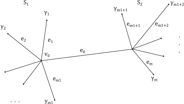
Figure 2: The tree graph considered in numerical tests.

Example 1. Consider a graph from Fig. 2 consisting of nine edges, $m=8$, $m_{1}=5$, the lengths of the edges $e_{0},\ldots,e_{8}$ are

$$L_{0}=1.4,\,L_{1}=\frac{e}{2},\,L_{2}=1,\,L_{3}=\frac{\pi}{2},\,L_{4}=\frac{\pi}{3},\,L_{5}=\frac{e^{2}}{4},\,L_{6}=1.1,\,L_{7}=1.2,\,L_{8}=1.$$ (7.1)

The corresponding nine components of the potential are defined as follows

$$\,q_{0}(x)=J_{0}(9x)+1,\,q_{1}(x)=\left|x-1\right|+1,\,q_{2}(x)=e^{-(x-\frac{1}{2})^{2}},\,q_{3}(x)=\sin\left(8x\right)+\frac{2\pi}{3},\,$$

$$q_{4}(x)=\cos\left(9x^{2}\right)+2,\,q_{5}(x)=\frac{1}{x+0.1},\,q_{6}(x)=\frac{1}{\left(x+0.1\right)^{2}},\,q_{7}(x)=e^{x},$$

$$\,q_{8}(x)=\left\{\begin{tabular}[c]{ll}$-35.2x^{2}+17.6x,$&$0\leq x<0.25$\\ $35.2x^{2}-35.2x+8.8,$&$0.25\leq x<0.75$\\ $-35.2x^{2}+52.8x-17.6,$&$0.75\leq x\leq 1,$\end{tabular}\ \ \ \ \right..$$

The potential $q_{8}(x)$ (from [14], [30]) is referred to below as saddle potential. To compute the Weyl matrix (direct problem) at a number of points $\rho_{k}^{2}$, we followed the approach from [6]. We took $180$ points $\rho_{k}$ chosen according to the rule $\rho_{k}=10^{\alpha_{k}}+0.1i$ with $\alpha_{k}$ being distributed uniformly on $\left[0,2\right]$. Such choice delivers a set of points which are more densely distributed near $\rho=1+0.1i$ and more sparsely near $\rho=100+0.1i$. In all our computations $N$ was chosen as $N=9$ (ten coefficients $g_{i,n}(L_{i})$ and ten coefficients $s_{i,n}(L_{i})$).

In Fig. 3 we show the exact potentials (continuous line) together with the recovered ones (marked with asterisks), computed with the proposed algorithm.

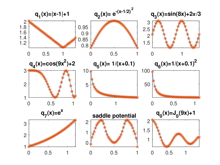
Figure 3: The potential of the quantum graph from Example 1, recovered from the Weyl matrix given at 180 points, with $N=9$.

Here the maximum relative error was attained in the case of the saddle potential, and it resulted in approximately $0.085$ in the vicinity of the endpoint $x=1$. All other potentials were computed considerably more accurately.

It is interesting to track how accurately the two spectra were computed on each edge. For example, Table 1 presents some of the “exact” Dirichlet-Dirichlet eigenvalues on $e_{2}$ computed with the aid of the Matslise package [26] (first column), the approximate eigenvalues, computed as described in subsection 5.2 by calculating zeros of $S_{2,9}(\rho,L_{2})$ and the absolute error of each presented eigenvalue. The zeros of $S_{2,9}(\rho,L_{2})$ were computed by converting this function into a spline on the interval $\left(0,650\right)$ and using the Matlab command fnzeros. Notice that both the absolute and relative errors remain remarkably small even for large indices.

Table 1: Dirichlet-Dirichlet eigenvalues of $q_{2}(x)$
$n$	$\lambda_{n}$	$\widetilde{\lambda}_{n}$	$\left|\lambda_{n}-\widetilde{\lambda}_{n}\right|$
$1$	$10.8381543818$	$10.8381543825$	$7.1\cdot 10^{-10}$
$11$	$1195.1450218516$	$1195.1450218560$	$4.4\cdot 10^{-9}$
$51$	$25671.7636244$	$25671.7636252$	$8.0\cdot 10^{-7}$
$101$	$100680.7570614$	$100680.7570623$	$9.4\cdot 10^{-7}$
$201$	$398742.8099714$	$398742.8099723$	$9.9\cdot 10^{-7}$

Similar results were obtained for the Neumann-Dirichlet eigenvalues.

It is interesting to observe how the error caused by the leaf peeling procedure is accumulated. For this we consider the second example, in which the potentials from the first sheaf are repeated on the second one.

Example 2. Consider a graph from Fig. 2 consisting of eighteen edges, $m=17$, $m_{1}=9$, the lengths of the edges $e_{1},\ldots,e_{9}$ are

$$L_{1}=\frac{e}{2},\,L_{2}=1,\,L_{3}=\frac{\pi}{2},\,L_{4}=\frac{\pi}{3},\,L_{5}=\frac{e^{2}}{4},\,L_{6}=1.1,\,L_{7}=1.2,\,L_{8}=1,\,L_{9}=1.4.$$

The corresponding eight components of the potential $q_{1}(x),\ldots,q_{8}(x)$ are defined as in the previous example, and additionally, $q_{9}(x)=J_{0}(9x)+1$. Next, $q_{i+9}(x)=q_{i}(x)$ and $L_{i+9}=L_{i}$ for $i=1,\ldots,8$, and $q_{0}(x)=q_{9}(x)$, $L_{0}=L_{9}$. That is, the nine components of the potential on the leaf edges of the first sheaf are all the potentials from the first example, the component of the potential on $e_{0}$ is that from Example 1, and eight components of the potential on the second sheaf are $q_{1}(x),\ldots,q_{8}(x)$ from Example 1. All other parameters were chosen as in Example 1. In Fig. 4 the result of the computation is presented. It is noteworthy that there is no considerable difference in the accuracy of the potentials recovered before applying the leaf peeling procedure (the first nine potentials) and after (the other nine ones). The largest difference is observed in the case of the potentials $q_{9}(x)$ and $q_{0}(x)$. Indeed, the maximum relative error for $q_{9}(x)$ resulted in approximately $0.003$ while for $q_{0}(x)$ in $0.175$ at the right endpoint. Interestingly enough, the accuracy of the recovery of all other potentials practically did not change after the leaf peeling procedure. For example, the maximum relative error for $q_{5}(x)$ was $0.037583$ while for its “twin” $q_{14}(x)$ it resulted in $0.037590$.

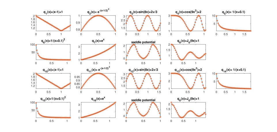
Figure 4: The potential of the quantum graph from Example 2, recovered from the Weyl matrix given at 180 points, with $N=9$.

Thus, the leaf peeling procedure does not lead to a considerable error accumulation and clearly can be applied several times that allows one to solve inverse problems on quite complicated tree graphs.

It is worth noting that the whole computation takes few seconds performed in Matlab 2017 on a Laptop equipped with a Core i7 Intel processor.

8 Conclusions

A new method for solving inverse problems on quantum tree graphs, consisting in the recovery of a potential from a Weyl matrix is developed. It is based on the leaf peeling method and Neumann series of Bessel functions representations for solutions of Sturm-Liouville equations. The given data are used for solving local inverse problems on sheaves, which in turn are reduced to separate two-spectra inverse Sturm-Liouville problems on leaf edges. The leaf peeling method allows one to remove the edges where the potential is already recovered and compute the Weyl matrix for the smaller tree. This combination of the leaf peeling method with the approach based on the Neumann series of Bessel functions representations results in a simple, direct and accurate numerical algorithm. Its performance is illustrated by numerical examples.

Funding The research of Sergei Avdonin was supported in part by the National Science Foundation, grant DMS 1909869, and by Moscow Center for Fundamental and Applied Mathematics. The research of Vladislav Kravchenko was supported by CONACYT, Mexico via the project 284470 and partially performed at the Regional mathematical center of the Southern Federal University with the support of the Ministry of Science and Higher Education of Russia, agreement 075-02-2022-893.

Data availability The data that support the findings of this study are available upon reasonable request.

Declarations

Conflict of interest The authors declare no competing interests.

References

- [1] Abramovitz M. and Stegun I. A. (1972), Handbook of mathematical functions, New York: Dover.
- [2] Arioli M. and Benzi M. (2018), A finite element method for quantum graphs. IMA J. Numer. Anal., 38, no. 3, 1119–1163.
- [3] Avdonin S., Belinskiy B. and Matthews J. (2011), Inverse problem on the semi-axis: local approach, Tamkang Journal of Mathematics, 42, no. 3, 1–19.
- [4] Avdonin S. and Bell J. (2015), Determining physical parameters for a neuronal cable model defined on a tree graph, Journal of Inverse Problems and Imaging, 9, no. 3, 645-659.
- [5] Avdonin S., Choque Rivero A., Leugering G. and Mikhaylov V. (2015), On the inverse problem of the two velocity tree-like graph, Zeit. Angew. Math. Mech., 95 , no. 12, 1490–1500.
- [6] Avdonin S. A., Khmelnytskaya K. V. and Kravchenko V. V. Recovery of a potential on a quantum star graph from Weyl’s matrix. arXiv:2210.15536.
- [7] Avdonin S. A. and Kravchenko V. V. (2023), Method for solving inverse spectral problems on quantum star graphs. Journal of Inverse and Ill-posed Problems, 31, no. 1, 31-42.
- [8] Avdonin S. and Kurasov P. (2008), Inverse problems for quantum trees, Inverse Problems and Imaging, 2, no. 1, 1–21.
- [9] Avdonin S., Leugering G. and Mikhaylov V. (2010), On an inverse problem for tree-like networks of elastic strings, Zeit. Angew. Math. Mech., 90, no. 2, 136–150.
- [10] Avdonin S. and Zhao Yu. (2021), Leaf peeling method for the wave equation on metric tree graphs. Inverse Probl. Imaging 15, no. 2, 185–199.
- [11] Baricz A., Jankov D. and Pogány T. K. (2017), Series of Bessel and Kummer-type functions. Lecture Notes in Mathematics, 2207. Springer, Cham.
- [12] Belishev M. and Vakulenko A. (2006), Inverse problems on graphs: Recovering the tree of strings by the BC-method, J. Inv. Ill-Posed Problems, 14 , 29-46.
- [13] Berkolaiko G. and Kuchment P. (2013), Introduction to Quantum Graphs, AMS, Providence, R.I.
- [14] Brown B. M., Samko V. S., Knowles I. W., Marletta M. (2003), Inverse spectral problem for the Sturm–Liouville equation, Inverse Probl. 19, 235–252.
- [15] Chadan Kh., Colton D., Päivärinta L., Rundell W. (1997), An introduction to inverse scattering and inverse spectral problems. SIAM, Philadelphia.
- [16] Karapetyants A. N. and Kravchenko V. V. (2022), Methods of mathematical physics: classical and modern. Birkhäuser, Cham.
- [17] Kravchenko V. V. (2019), On a method for solving the inverse Sturm–Liouville problem, J. Inverse Ill-posed Probl. 27, 401–407.
- [18] Kravchenko V. V. (2020), Direct and inverse Sturm-Liouville problems: A method of solution, Birkhäuser, Cham.
- [19] Kravchenko V. V. (2022), Spectrum completion and inverse Sturm-Liouville problems. Math Meth Appl Sci.; 1-15. doi:10.1002/mma.8869.
- [20] Kravchenko V. V., Khmelnytskaya K. V. and Çetinkaya F. A. (2022), Recovery of inhomogeneity from output boundary data, Mathematics, 10, 4349, https://doi.org/10.3390/math10224349.
- [21] Kravchenko V. V., Navarro L. J. and Torba S. M. (2017), Representation of solutions to the one-dimensional Schrödinger equation in terms of Neumann series of Bessel functions, Appl. Math. Comput. 314, 173–192.
- [22] Kravchenko V. V. and Torba S. M. (2015), Analytic approximation of transmutation operators and applications to highly accurate solution of spectral problems, Journal of Computational and Applied Mathematics 275, 1-26.
- [23] Kravchenko V. V. and Torba S. M. (2021), A direct method for solving inverse Sturm-Liouville problems, Inverse Probl. 37, 015015 (32pp).
- [24] Kravchenko V. V. and Torba S. M. (2021), A practical method for recovering Sturm-Liouville problems from the Weyl function, Inverse Probl. 37, 065011 (26pp).
- [25] Kurasov P. and Nowaczyk M. (2005), Inverse spectral problem for quantum graphs, J. Phys. A., 38, 4901-4915.
- [26] Ledoux V., Daele M.V. and Berghe G.V. (2005), MATSLISE: a MATLAB package for the numerical solution of Sturm–Liouville and Schrödinger equations, ACM Trans. Math. Softw. 31, 532–554.
- [27] Levitan B. M. (1987), Inverse Sturm-Liouville problems, VSP, Zeist.
- [28] Marchenko V. A. (2011), Sturm-Liouville operators and applications: revised edition, AMS Chelsea Publishing.
- [29] Mugnolo D. (2014), Semigroup Methods for Evolution Equations on Networks, Understanding Complex Systems, Springer, Cham.
- [30] Rundell W. and Sacks P. E. (1992), Reconstruction techniques for classical inverse Sturm–Liouville problems, Math. Comput. 58, 161–183.
- [31] Shishkina E. L. and Sitnik S. M. (2020), Transmutations, singular and fractional differential equations with applications to mathematical physics, Elsevier, Amsterdam.
- [32] Savchuk A. M., Shkalikov A. A. (2005), Inverse problem for Sturm–Liouville operators with distribution potentials: reconstruction from two spectra, Russ. J. Math. Phys. 12, 507–514.
- [33] Watson G. N. (1996), A Treatise on the theory of Bessel functions, 2nd ed., reprinted, Cambridge University Press, Cambridge.
- [34] Wilkins J. E. (1948), Neumann series of Bessel functions. Trans. Amer. Math. Soc. 64, 359–385.
- [35] Yurko V. A. (2005), Inverse Sturm-Lioville operator on graphs, Inverse Problems, 21, 1075-1086.
- [36] Yurko V. A. (2007), Introduction to the theory of inverse spectral problems, Fizmatlit, Moscow, (in Russian).