Controllable quantum scars induced by spin-orbit couplings in quantum dots

Abstract

The spin-orbit couplings (SOCs) which are the relativistic corrections originated from the Dirac equation, offer nonlinearity in the classical limit and are capable of driving the chaotic dynamics. In a quantum dot confined by a two dimensional parabolic potential with SOCs, various quantum scar states emerge quasi-periodically in the eigenstates of the system, when the ratio of the confinement energies in the two directions are nearly commensurable. The scars, displaying both the quantum interference and the classical trajectory on the electron density, induced by the relativistic effects, indicate the bridge between the classical and quantum behaviors of the system. When the strengths of the Rashba and Dresselhaus SOCs are identical, the chaos is eliminated as the classical Hamilton’s equations being linear and all the quantum scar states disappear consequently. The quantum scars induced by SOCs are found to be robust against small perturbations of the systematic parameters. As the Rashba SOC been controlled precisely by an external gate in experiments, the quantum scar here is fully predictable, controllable and accessible to detection.

Quantum scars which are the localization behavior displaying certain unstable classical periodic orbits exist in the high-energy levels in the quantum system with chaotic dynamics being driven in its classical limit. The quantum scar was first discovered while studying the quantum eigenstates of the stadium billiard model which drives chaotic dynamics in the corresponding classical model [1] and later was named as such by Heller [2]. Quantum scarring has thus far drawn great attention and interest [3] and has been observed experimentally in various systems, including quantum well and microwave resonators [4] and in graphene nanostructures. The localization nature in the quantum scarring without participation of the many-body system is convenient to be applied and is interested in many fields. On the other hand, the quantum many-body scars localizing the eigenstates to prevent thermalization are expected to be useful in quantum computing [5].

Recently, the perturbation induced quantum scars have been studied in the quantum dot (QD) systems confined at the semiconductor heterostructure with or without an external magnetic field [6, 7, 8]. These quantum scars are induced by a bunch of impurities which make the (nearly) degenerate states of the QD resonant to localize the electron density along the underlying classical trajectories. As an artificial atom [9], the low-dimensional QD [10, 11, 12, 13, 14] is an ideal platform to control both the spin and the charge of a single or many electrons. The parabolic confinements of the QD make the system a two-dimensional (2D) quantum harmonic oscillator which has practical and fundamental meanings in physics. The quantum scars found in QDs also reveal the profound links between the classical and the quantum systems.

Both the nonrelativistic and the relativistic quantum systems have been found to possess the quantum scars [15]. The focus has also been on quantum scarring in systems described by the Dirac equation, especially in graphene systems [16]. Moreover, the spin-orbit coupling (SOC) is also a relativistic effect which is the correction originated from the Dirac equation, and its corresponding classical Hamiltonian leads to nonlinearity in Hamilton’s equation and it is possible to drive the chaotic dynamics [17]. However, the study of the quantum scar induced by the SOCs could be an interesting route [18]. The studies on the QDs with Rashba or/and Dresselhaus SOCs have been reported extensively thus far [19, 20, 21, 22, 23, 24, 25, 26, 27, 28, 29, 30, 31, 32, 33, 34]. The ground states of the QDs with SOCs have been studied to explore the topological nontrivial features in the spin fields [35, 36, 37]. Vortex-like spin textures in the ground states carry different topological charges induced by Rashba or Dresselhaus SOC. Considering that the Rashba SOC is convenient to tune via an external gate [38, 39, 40, 41, 42], the spin textured ground states there could have potential applications in spintronics and quantum information [43, 44, 45]. Yet, the excited states in QDs with SOCs are not sufficiently studied, especially in the energy region containing the classical chaos.

Here we investigate the excited states as well as the quantum scarring in spin-orbit coupled QDs appearing quasi-periodically in the eigenstates. We also confirm that the condition of scarring the quantum states exactly follows the chaos condition in the classical limit. It is worth mentioning that the quantum scars induced by SOCs in QDs are even more robust against small perturbations, more tunable, less random, exist at low-energy levels, and spin-involved, comparing with the impurities induced quantum scar. We thus expect the corresponding measurements to be more convenient by scanning tunneling spectroscopy [46], the NMR experiment [47] and the spin-dependent transport [18, 48].

The Hamiltonian of the QD with both the Rashba and Dresselhauss SOCs is given by

$$\mathcal{H}=\frac{\mathbf{P}^{2}}{2m^{\ast}}+\frac{m^{\ast}}{2}\left(\omega_{x}^{2}x^{2}+\omega_{y}^{2}y^{2}\right)+\frac{\Delta}{2}\sigma_{z}+\mathcal{H}_{SOC},$$ (1)

$$\mathcal{H}_{SOC}=g_{1}\left(\sigma_{x}P_{y}-\sigma_{y}P_{x}\right)+g_{2}\left(\sigma_{y}P_{y}-\sigma_{x}P_{x}\right),$$ (2)

where $\omega_{x}$ and $\omega_{y}$ describe the parabolic confinements in $x$ and $y$ dimensions, respectively. $\sigma_{i}$ is the Pauli matrix and the strengths of the Rashba and Dresselhas SOCs are $g_{1}$ and $g_{2}$ respectively. $P_{i}=p_{i}+eA_{i}$ is the kinetic momentum, where $e$ is the charge of an electron and the vector potential can be chosen in the symmetric gauge $\mathbf{A}=\frac{1}{2}B\left(-y,x,0\right)$ in magnetic field $B.$ The Zeeman termis $\Delta=g\mu_{B}B$, where $g$ is the Landé factor and $\mu_{B}$ is the Bohr magneton.

In the adiabatic model the SOCs could have a classical correspondence [17] which provides nonlinearity and is able to drive chaotic dynamics. The classical Hamiltonian, without a magnetic field, reads

$$H^{C} = \frac{(p_{x}^{\prime})^{2}+(p_{y}^{\prime})^{2}}{2m^{*}}+\frac{1}{2}m^{*}\omega_{x}^{2}x^{2}+\frac{1}{2}m^{*}\omega_{y}^{2}y^{2}$$ (3)

$$- \sqrt{\left(g_{1}+g_{2}\right)^{2}(p_{x}^{\prime})^{2}+\left(g_{1}-g_{2}\right)^{2}(p_{y}^{\prime})^{2}},$$

where $p^{\prime}_{x}=(p_{y}-p_{x})/\sqrt{2}$ and $p^{\prime}_{y}=(p_{x}+p_{y})/\sqrt{2}$. By solving the canonical equations, the chaotic dynamics can appear. Note that if the confinement trap is isotropic, the classical trajectories in the phase space would be regular. The way to induce chaotic dynamics is to make the confinement anisotropic or to make the SOCs anisotropic. Once the chaos appears, the corresponding quantum scar should be found in the QD induced by the SOC. Note that the classical behavior for whichever SOC is the same, implying the quantum scar induced by either SOC to be identical.

To study the quantum scar of the QD system described by the Hamiltonian (1), the eigenstates are calculated in the exact diagonalization scheme. The Hamiltonian matrix is constructed in the basis of 2D quantum oscillator whose Hamiltonian is $H_{0}=\frac{\mathbf{p}^{2}}{2m^{\ast}}+\frac{m^{\ast}}{2}\left(\Omega_{x}^{2}x^{2}+\Omega_{y}^{2}y^{2}\right)+\frac{\Delta}{2}\sigma_{z}$, where the renormalized frequency is defined as $\Omega_{x,y}=\sqrt{\omega_{x,y}^{2}+\omega_{c}^{2}/4}$ with the cyclotron frequency in a magnetic field $\omega_{c}=|e|B/m^{*}$. The basis of the 2D quantum oscillator is $|k\rangle\equiv|k_{x},k_{y},k_{s}\rangle$ with its wavefunction $\psi_{k_{x},k_{y}}(\mathbf{r})$ [49] where $k$ is a collective index marking the number of the basis, $k_{s}$ is its spin index, and $k_{x,y}$ denote the two quantum numbers of the 2D quantum oscillator.

In practice, a truncation of $k_{x,y}$ is necessary and the low-energy states can be found accurately. Once the Hamiltonian (1) is diagonalized, the $m-$th eigenstate can be expressed by the basis, $|\Psi_{m}\rangle=\sum_{i}C_{i}^{m}|i\rangle$, and its wave function is $\Psi_{m}(\mathbf{r})=\langle\mathbf{r}|\Psi_{m}\rangle=\sum_{i}C^{m}_{i}\psi_{i_{x},i_{y}}(\mathbf{r})|i_{s}\rangle$. Generally, any observable field is given by $\Lambda(\mathbf{r})=\Psi_{m}^{\dagger}(\mathbf{r})\Lambda\Psi_{m}(\mathbf{r}),$ where $\Lambda$ is the corresponding operator including the density operator $n$ (unity matrix), spin operators $\sigma_{x,y,z}$, current operators and etc.

Without loss of generality, we consider the InAs quantum dots with the material parameters: the effective mass of electron $m^{\ast}=0.042m_{e}$ where $m_{e}$ is the mass of free electron and Landé factor $g=-14$. The size of the QD is not fixed here, but we could fix the confinement in the $x$ direction and vary the other confinement. The confinement lengths are given by $R_{i}=\sqrt{\hbar/m^{*}\omega_{i}}$ and $R_{x}$ is fixed to $30$ nm associated with the characterized confinement energy $\hbar\omega_{x}\approx 2$ meV.

When there is only one SOC present and the QD is isotropic, $\omega_{x}=\omega_{y}$, the associated classical Hamiltonian does not lead to chaos. In the quantum regime, the densities and the spin fields of all the eigenstates of the isotropic QD are deformed by the SOC. The rotational symmetry does not only exist in the ground state, but also exists in all the excited states of the single-particle system, due to the symmetry $[L_{z}\pm\sigma_{z}/2,\mathcal{H}]=0$, where $L_{z}$ is the $z$ component of the angular momentum [35]. The topological feature of the spin fields is also retained in the excited states, i.e. nontrivial patterns with a nonzero topological charge are textured by the SOC [35, 36], more details can be found in the supplementary materials (SM) [49].

The chaotic dynamics can be driven in the isotropic dot by combining the two SOCs arbitrarily, $|g_{1}|\neq|g_{2}|$. The canonical equations are nonlinear and possible to lead chaotic dynamics. In the quantum regime, the quantum scars represented by the electron density localizing along the classical trajectory can appear in the excited states. The absence of the magnetic field conserves the time reversal symmetry and the quantum scar states appear in pair due to the Kramers pair. In Fig. 1, we show two quantum scars in the excited states of an isotropic QD with the combination of the Rashba and the Dresselhaus SOCs, $\hbar g_{1}=40$ nm$\cdot$meV and $\hbar g_{2}=10$ nm$\cdot$meV. In Fig. 1(a), the density is localized to an axe-shape while an ‘X’-trajectory appears in Fig. 1(b), which are different from the array-shape quantum states in a QD without SOC significantly.

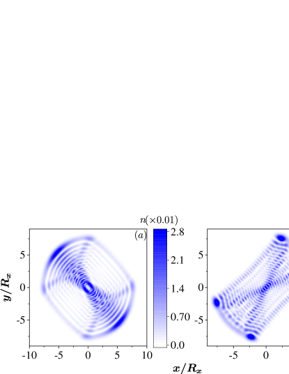
Figure 1: (Color online) The quantum scar states in an isotropic QD ($R_{x,y}=30$ nm) with mixing of the two SOCs, $\hbar g_{1}=40$ nm$\cdot$meV and $\hbar g_{2}=10$ nm$\cdot$meV. In (a) and (b), the color represents the densities of the electron $n(\mathbf{r})$ in the 1028th and 1247th eigenstates, respectively.

Another quantum scar called quantum Lissajous scar [8] can emerge in an anisotropic QD where the ratio of the 2D confinements $\omega_{x}/\omega_{y}$ is a rational number. The original idea to realize the quantum Lissajous scars is by the massive random impurities which induce chaos and mix different eigenstates of the basis. The scar indicates the classical trajectory of the anisotropic 2D oscillator, and the density of the electron of the quantum scar localizes around the related Lissajous curve.

Here, we demonstrate that the quantum Lissajous scars can be achieved by the relativistic correction, i.e., the SOC. In an anisotropic QD, the corresponding classical Hamiltonian also leads to chaotic dynamics in the phase space obtained by its Hamilton’s equation. The dimensionless Hamiltonian $H^{C}=p_{x}^{2}+p_{y}^{2}+\frac{1}{2}\omega_{x}^{2}x^{2}+\frac{1}{2}\omega_{y}^{2}y^{2}-g_{1(2)}\sqrt{p_{x}^{2}+p_{y}^{2}}$ without magnetic field possesses positive Lyapunov exponent (LE) demonstrating chaos in the system at some energies [49, 50].

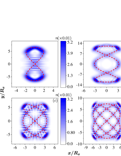
Figure 2: (Color online) The quantum scar states in anisotropic QDs ($R_{x}=30$ nm) with only the Rashba SOC, $\hbar g_{1}=40$ nm$\cdot$meV. Colors represent for the density of the electron, $n(\mathbf{r})$. The dashed lines are the corresponding Lissajous curves $(\cos\eta_{x}t,\cos(\eta_{y}t+\frac{\pi}{2\eta_{x}}))$ with $\omega_{x,y}=\eta_{x,y}\omega_{0}$ drawn for guidance. (a) The quantum scar in the $91$st eigenstate in the QD with $R_{y}=\sqrt{2}R_{x}$ and $\omega_{x}/\omega_{y}=2/1$. (b) For the QD with $R_{y}=\sqrt{3}R_{x}$ and $\omega_{x}/\omega_{y}=3/1$, the quantum scar in the $535$th eigenstate. (c) $R_{y}=\sqrt{3/2}R_{x}$ and $\omega_{x}/\omega_{y}=3/2$, the quantum scar in the $331$st eigenstate. (d) $R_{y}=\sqrt{4/3}R_{x}$ and $\omega_{x}/\omega_{y}=4/3$, the quantum scar in the $1404$th eigenstate.

In the quantum regime, the emerging quantum scars also display the trajectory of a particle confined in a classical 2D oscillator. We note that the quantum Lissajous scars here are related to the specific closed Lissajous curves, $(\cos\eta_{x}t,\cos(\eta_{y}t+\frac{\pi}{2\eta_{x}}))$, where $\omega_{x,y}=\eta_{x,y}\omega_{0}$. The quantum Lissajous scars for $\omega_{x}/\omega_{y}=2/1,3/1,3/2,4/3$ are shown in Figs. 2(a)-(d), respectively. Around the cross points in the curves, the interference stripes are clearly visible, indicating both the classical and quantum features. More density profiles can be found in the video in the SM [49].

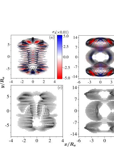
Figure 3: (Color online) (a) - (b) The spin fields and (c) - (d) the associated current fields $(j_{x}(\mathbf{r}),j_{y}(\mathbf{r}))$ of the quantum scar states shown in Figs. 2(a) - (b). Colors in (a) and (b) represent $\sigma_{z}(\mathbf{r})$ and the vectors represent the in-plane spin fields $(\sigma_{x}(\mathbf{r}),\sigma_{y}(\mathbf{r}))$.

In Figs. 3(a) - (d), we also show the associated spin and the current fields of the two quantum Lissajous scars [Figs. 2(a) - (b)], respectively. The spin textures are difficult to calculate analytically, we obtain numerically the in-plane spins textured with nontrivial pattern. There are many vortices localized associated with the density profile, which are textured by the SOC. The flow direction of the current, shown in Figs. 3(c) and (d) is not along the classical Lissajous trajectory, but is relevant to the spin fields shown in Figs. 3(a) and (b). It also indicates the fundamental difference between the classical and the quantum mechanism.

It is worth noting that some eigenstates do not show any different density profile other than the regular dot-array ones of the 2D quantum oscillator without the SOC. It is because in the corresponding energy region, the classical dynamics can be regular with zero LE, and as a result, the associated quantum states show no scar. The chaotic behavior induced by the SOC is significantly different from that induced by random impurities, and so are the quantum scar states.

Due to the randomness of the sizes and the locations of the impurities, the quantum scars can not be tracked precisely in the QD with impurities, and only the percentage of the scar states in all eigenstates can be approximately estimated. It makes the detection of the scar states difficult. In contrast, in an anisotropic QD with the SOC, the emerging quantum scars are not random and can be accurately predicted. Each two quantum Lissajous scar states (due to the Kramers pair) quasi-periodically appear in every a few eigenstates. There are about 12 states between the two pairs of the quantum Lissajous scar states in the case of $\omega_{x}/\omega_{y}=3/2$, but the period is not fixed and will be increased gradually (not monotonically) with the increase of the energies. Moreover, the quantum Lissajous scars induced by the SOC can be found at very low energies. For instance, the ‘$8$’-shape Lissajous trajectory shown in Fig. 2(a) can be found even down to the $15$th eigenstate [49]. More importantly, the Rashba SOC can be controlled by the external gate, thus the quantum scar states can be controlled. The above features of the quantum scars imply that the SOC (especially the tunable Rashba SOC) brings great convenience on the measurement of the quantum scar state.

However, due to the nature of the chaotic dynamics being sensitive to the initial conditions, ones wonder if the quantum scars are sensitive to the system parameters. If not, the quantum scar states are more easily detected. We tune the confinement ratio slightly, for instance, $\omega_{x}/\omega_{y}=3/2\rightarrow 3.01/2$. The positions of the quantum scar states in all the eigenstates are not changed at all, neither are their density profiles. We then test the effect of adding a weak magnetic field, $B=0.05$ T. The Kramers pair is lifted and the quantum scars still exist in the same eigenstates as the case without the magnetic field. Only the density profiles are slightly changed. If the Rashba SOC strength $g_{1}$ is tuned a little, the positions or the density profiles of the quantum scar states remain unchanged [49].

The robustness of the quantum scars against the external perturbations relies on the quantum properties of the system rather than its classical behavior. It can also be boiled down to the fact that the small perturbation does not change too much the eigenenergies of the eigenstates, so that the corresponding classical behavior is unchanged (still in the chaos/regular region) and the scarring is frozen in the discrete-energy quantum system. This property is also helpful for fixing the quantum scar states to make the possible measurement convenient.

In anisotropic QDs with one SOC, the Lissajous patterns in open curves can also be found in the scarring states, but in a much lower probability. However, due to the mirror symmetry, $(x,y)\rightarrow-(x,y)$ without a magnetic field, a single open curve of Lissajous pattern with lower symmetry can not be found. Only a pair of the Lissajous curves making up this symmetry emerges in a scarred state. In QDs with $\omega_{x}/\omega_{y}=2/1,3/1,3/2,4/3$, the pairs of the scarred Lissajous curves are indicated in Figs. 4(a) - (d), where the classical orbits $(\cos\eta_{x}t,\cos\eta_{y}t)+(\cos\eta_{x}t,\cos(\eta_{y}t+\pi/\eta_{x}))$ are identified, respectively.

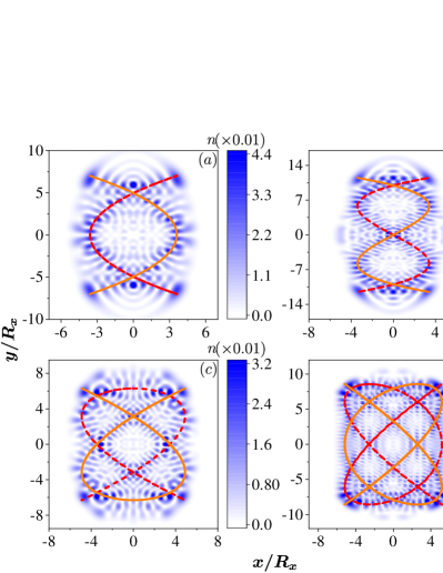
Figure 4: (Color online) The Lissajous curves pairs in the quantum scar states in the anisotropic QD with the same systematic parameters as those used in Fig. 2. Colors represent the density of the electron. The quantum scars in (a) the $417$th eigenstate with $\omega_{x}/\omega_{y}=2/1$, (b) the $659$th eigenstate with $\omega_{x}/\omega_{y}=3/1$, (c) the $705$th eigenstate with $\omega_{x}/\omega_{y}=3/2$, and (d) the $1571$st eigenstate with $\omega_{x}/\omega_{y}=4/3$. The lines are the corresponding Lissajous curves drawn for guidance.

Considering that the classical Hamiltonians are identical for Rashba and Dresselhaus SOCs, the density profiles of the quantum scar states induced by either one of the two SOCs are identical: Suppose that there are two identical QDs, one with Rashba SOC and the other one with Dresselhaus SOC. The coupling strengths are equal. Our numerical studies show that the quantum scar states appear in the same position in the eigenstates of the two cases with exactly the same density profiles. However, the spin fields of these two states are different, which can be used to distinguish the type of the SOC.

Finally, we discuss the effect of the combination of the two SOCs in anisotropic QDs. As expected, when $g_{1}\neq\pm g_{2}$, the quantum Lissajous scars appear, as distorted pattern of the case with only one SOC. The special case that $|g_{1}|=|g_{2}|$ has the classical correspondence of a linear system, $H^{C}=\frac{1}{2m^{*}}[(p^{\prime}_{x})^{2}+(p_{y}^{\prime})^{2}]+\frac{1}{2}m^{*}(\omega_{x}^{2}x^{2}+\omega_{y}^{2}y^{2})-2|g_{1}|p^{\prime}_{x}.$ Thus, whatever the QD is isotropic or anisotropic, neither classical chaotic dynamics nor quantum scar appears. Our numerical calculation also confirms that all the density profiles of the eigenstates are alike dot-array, which are the same as the densities of the eigenstates of the QD without SOC, induced by the Hermite polynomials in the basis wavefunctions. The difference of the two cases is that the spin fields are nonzero in the QD with SOCs, but are polarized in $z$ direction in the QD without SOC [49]. When a magnetic field increases, the scars are overwhelmed by the cyclotron motion.

In summary, we have studied the quantum scar states in QDs induced by the relativistic effect, i.e., the SOC. For isotropic QDs, only the mixing of the Rashba and Dresselhaus SOCs, which leads to chaotic dynamics, can induce quantum scars. In an anisotropic QD, either one or combination of the two SOCs leads to quantum Lissajous scar which contains one or a pair of Lissajous curves. In a special case, $g_{1}=\pm g_{2}$, corresponding to a linear classical system without chaos, whatever the confinement of the QD is, no quantum scar appears.

The quantum scaring induced by the SOC is robust against small variations of the external conditions, such as weak magnetic field, perturbations of the confinement ratio $\omega_{x}/\omega_{y}$ and the SOCs. The quantum Lissajous scars induced by the SOCs emerge quasi-periodically in the eigenstates and can be formed at very low energies. It implies that tuning the SOC is a stable and controllable way to obtain the quantum scar, not as the systems with the quantum scars being induced by randomness. The direct observation of the orbit of the ground state of a QD is already realized [51], our work paves the way to observe the quantum scars directly, since all these states are predictable. If direct observation is difficult, other indirect detection, such as spin polarization measurement, may be also useful. Especially, the transport signals could be utilized to determine the scarring trajectory in the QDs with the SOCs, and the spin-involved transport is also potentially helpful for the application of spintronics.

Acknowledgement. W.L. acknowledges Chao Hang for helpful discussions. This work is supported by the NSF-China under Grant Nos. 11804396 and 62071496. We are grateful to the High Performance Computing Center of Central South University for partial support of this work.

References

- [1] S.W. McDonald and A. N. Kaufman, Phys. Rev. Lett. 42, 1189 (1979); Phys. Rev. A 37, 3067 (1988).
- [2] E. J. Heller, Phys. Rev. Lett. 53, 1515 (1984).
- [3] E. B. Bogomolny, Physica (Amsterdam) 31D, 169 (1988); M.V. Berry, Proc. R. Soc. A 423, 219 (1989); M. C. Gutzwiller, Chaos in Classical and Quantum Mechanics (Springer, New York, 1990); H. J. Stöckmann, Quantum Chaos: An Introduction (Cambridge University Press, Cambridge, England, 1999).
- [4] S. Sridhar, Phys. Rev. Lett. 67, 785 (1991); J. Stein and H.-J. Stöckmann, Phys. Rev. Lett. 68, 2867 (1992); T. M. Fromhold, P. B. Wilkinson, F.W. Sheard, L. Eaves, J. Miao, and G. Edwards, Phys. Rev. Lett. 75, 1142 (1995); P. B.Wilkinson, T. M. Fromhold, L. Eaves, F.W. Sheard, N. Miura, and T. Takamasu, Nature (London) 380, 608 (1996); S.-B. Lee, J.-H. Lee, J.-S. Chang, H.-J. Moon, S.W. Kim, and K. An, Phys. Rev. Lett. 88, 033903 (2002); T. Harayama, T. Fukushima, P. Davis, P. O. Vaccaro, T. Miyasaka, T. Nishimura, and T. Aida, Phys. Rev. E 67, 015207(R) (2003).
- [5] H. Bernien, S. Schwartz, A. Keesling, H. Levine, A. Omran, H. Pichler, S. Choi, A. S. Zibrov, M. Endres, M. Greiner, V. Vuletić and M. D. Lukin, Nature 551, 579 (2017); C. J. Turner, A. A. Michailidis, D. A. Abanin, M. Serbyn and Z. Papić, Nat. Phys. 14, 745 (2018); Wen Wei Ho, Soonwon Choi, Hannes Pichler, and Mikhail D. Lukin, Phys. Rev. Lett. 122, 040603 (2019); P. Zhang, H. Dong, Y. Gao, L. Zhao, J. Hao, J.-Y. Desaules, Q. Guo, J. Chen, J. Deng, B. Liu, W. Ren, Y. Yao, X. Zhang, S. Xu, K. Wang, F. Jin, X. Zhu, B. Zhang, H. Li, C. Song, Z. Wang, F. Liu, Z. Papić, L. Ying, H. Wang and Y.-C. Lai, Nat. Phys. (2022).
- [6] P. J. J. Luukko, B. Drury, A. Klales, L. Kaplan, E. J. Heller, and E. Räsänen, Sci. Rep. 6, 37656 (2016).
- [7] J. Keski-Rahkonen, P. J. J. Luukko, L. Kaplan, E. J. Heller, and E. Räsänen, Phys. Rev. B 96, 094204 (2017).
- [8] J. Keski-Rahkonen, A. Ruhanen, E. J. Heller, and E. Räsänen, Phys. Rev. Lett. 123, 214101 (2019).
- [9] P.A. Maksym, and T. Chakraborty, Phys. Rev. Lett. 65, 108 (1990).
- [10] T. Chakraborty, Quantum Dots (Elsevier, Amsterdam 1999).
- [11] D. Bimberg, M. Grundmann, and N. N. Ledentsov, Quantum Dot Heterostructures (John Wiley and Sons, Chichester, 1999).
- [12] L. P. Kouwenhoven, D. G. Austing, and S. Tarucha, Rep. Prog. Phys. 64, 701-736 (2001).
- [13] R. Hanson, L. P. Kouwenhoven, J. R. Petta, S. Tarucha, and L. M. K. Vandersypen, Rev. Mod. Phys. 79, 1217 (2007).
- [14] C. Kloeffel, and D. Loss, Annu. Rev. Condens. Matter Phys. 4, 51 (2013).
- [15] Hongya Xu, Liang Huang, Ying-Cheng Lai, and Celso Grebogi, Phys. Rev. Lett. 110, 064102 (2013); Liang Huang, Hong-Ya Xu, CelsoGrebogi, and Ying-ChengLai, Physics Reports 753, 1 (2018).
- [16] Liang Huang, Ying-Cheng Lai, David K. Ferry, Stephen M. Goodnick, and Richard Akis, Phys. Rev. Lett. 103, 054101 (2009); Damien Cabosart, Alexandre Felten, Nicolas Reckinger, Andra Iordanescu, Sébastien Toussaint, Sébastien Faniel and Benoît Hackens, Nano Lett. 17, 1344 (2017); G. Q. Zhang, Xianzhang Chen, Li Lin, Hailin Peng, Zhongfan Liu, Liang Huang, N. Kang, and H. Q. Xu, Phys. Rev. B 101, 085404 (2020); Hong-Ya Xu, Liang Huang, and Ying-Cheng Lai, Physics Today 74, 44 (2021).
- [17] Jonas Larson, Brandon M. Anderson, and Alexander Altland, Phys. Rev. A 87, 013624 (2013).
- [18] Michael Berger, Dominik Schulz and Jamal Berakdar, Nanomaterials 11, 1258 (2021).
- [19] O. Voskoboynikov, C. P. Lee, and O. Tretyak, Phys. Rev. B 63, 165306 (2001).
- [20] M. Governale, Phys. Rev. Lett. 89, 206802 (2002).
- [21] A. Emperador, E. Lipparini, and F. Pederiva, Phys. Rev. B 70, 125302 (2004).
- [22] D. V. Bulaev, and D. Loss, Phys. Rev. B 71, (2005).
- [23] S. Weiss and R. Egger, Phys. Rev. B 72, 245301 (2005).
- [24] T. Chakraborty, and P. Pietiläinen, Phys. Rev. Lett. 95, 136603 (2005); P. Pietiläinen, and T. Chakraborty, Phys. Rev. B 73, 155315 (2006).
- [25] A. Ambrosetti, F. Pederiva, and E. Lipparini, Phys. Rev. B 83, 155301 (2011).
- [26] C. F. Destefani, S. E. Ulloa, and G. E. Marques, Phys. Rev. B 69, 125302 (2004).
- [27] T. Chakraborty, and P. Pietiläinen, Phys. Rev. B 71, 113305 (2005).
- [28] A. Cavalli, F. Malet, J. C. Cremon, and S. M. Reimann, Phys. Rev. B 84, 235117 (2011).
- [29] E. Tsitsishvili, G. S. Lozano, and A. O. Gogolin, Phys. Rev. B 70, 115316 (2004).
- [30] S. K. Ghosh, Jayantha P. Vyasanakere, and V. B. Shenoy, Phys. Rev. A 84, 053629 (2011).
- [31] Yi Li, Xiangfa Zhou, and Congjun Wu, Phys. Rev. B 85, 125122 (2012).
- [32] S. Avetisyan, Pekka Pietiläinen, and Tapash Chakraborty, Phys. Rev. B 88, 205310 (2013).
- [33] S. D. Ganichev, V. V. Bel’kov, L. E. Golub, E. L. Ivchenko, Petra Schneider, S. Giglberger, J. Eroms, J. De Boeck, G. Borghs, W. Wegscheider, D. Weiss, and W. Prettl, Phys. Rev. Lett. 92, 256601 (2004).
- [34] G. A. Intronati, P. I. Tamborenea, D. Weinmann, R. A. Jalabert, Phys. Rev. B 88, 045303 (2013).
- [35] Wenchen Luo, Amin Naseri, Jesko Sirker, and Tapash Chakraborty, Sci. Rep. 9, 672 (2019).
- [36] Wenchen Luo and Tapash Chakraborty, Phys. Rev. B 100, 085309 (2019).
- [37] Amin Naseri, Shenglin Peng, Wenchen Luo, and Jesko Sirker, Phys. Rev. B 101, 115407 (2020).
- [38] J. Nitta, T. Akazaki, H. Takayanagi, and T. Enoki, Phys. Rev. Lett. 78, 1335 (1997).
- [39] M. Kohda, T. Bergsten, and J. Nitta, J. Phys. Soc. Jpn. 77, 031008 (2008).
- [40] C. R. Ast, D. Pacilé, L. Moreschini, M. C. Falub, M. Papagno, K. Kern, M. Grioni, J. Henk, A. Ernst, S. Ostanin, and P. Bruno, Phys. Rev. B 77, 081407(R) (2008).
- [41] Y. Kanai, R. S. Deacon, S. Takahashi, A. Oiwa, K. Yoshida, K. Shibata, K. Hirakawa, Y. Tokura, and S. Tarucha, Nat. Nanotechnol. 6, 511 (2011).
- [42] M. P. Nowak, B. Szafran, F. M. Peeters, B. Partoens, and W. J. Pasek, Phys. Rev. B 83, 245324 (2011).
- [43] I. Zutic, J. Fabian, and S. Das Sarma, Rev. Mod. Phys. 76, 323 (2004).
- [44] L. Smejkal, Y. Mokrousov, Binghai Yan, and A. H. MacDonald, Nat. Phys. 14, 242 (2018).
- [45] O. Gomonay, T. Jungwirth, and J. Sinova, Phys. Stat. Sol. RRL 11, 1700022 (2017).
- [46] J. Velasco Jr., J. Lee, D. Wong, S. Kahn, H.-Z. Tsai, J. Costello, T. Umeda, T. Taniguchi, K. Watanabe, A. Zettl, F. Wang, and M. F. Crommie, Nano Lett. 18, 5104 (2018); N. M. Freitag, T. Reisch, L. A. Chizhova, P. Nemes-Incze, C. Holl, C. R. Woods, R. V. Gorbachev, Y. Cao, A. K. Geim, K. S. Novoselov, J. Burgdörfer, F. Libisch & M. Morgenstern, Nat. Nanotechnol. 13, 392 (2018).
- [47] A.E. Dementyev, P. Khandelwal, N. N. Kuzma, S.E. Barrett, L. N. Pfeiffer, K. W. West, Solid State Comm. 119, 217 (2001); N. N. Kuzma, P. Khandelwal, S. E. Barrett, L. N. Pfeiffer, K. W. West, Science 281, 686 (1998); S. E. Barrett, G. Dabbagh, L. N. Pfeiffer, K. W. West, and R. Tycko, Phys. Rev. Lett. 74, 5112 (1995).
- [48] Jian Sun, Russell S. Deacon, Xiaochi Liu, Jun Yao, and Koji Ishibashi, Appl. Phys. Lett. 117, 052403 (2020); Shenglin Peng, Fangping Ouyang, Jian Sun, Ai-Min Guo, Tapash Chakraborty, and Wenchen Luo, Appl. Phys. Lett. 118, 082402 (2021); Zhongwang Wang, Yahua Yuan, Xiaochi Liu, Manoharan Muruganathan, Hiroshi Mizuta, and Jian Sun, Appl. Phys. Lett. 118, 083105 (2021).
- [49] More details can be found in the supplementary materials. The evolutions of the density profiles of increasing eigenstates integrated in a video is also provided therein.
- [50] Z. Yao, K. Sun, S. He, Nonlinear Dynamics 110, 1807 (2022).
- [51] L. C. Camenzind, L. Yu, P. Stano, Zimmerman, A. C. Gossard, D. Loss, and D. M. Zumbühl, Phys. Rev. Lett. 122, 207701 (2019).