Cross-Modal Fine-Tuning: Align then Refine

Abstract

Fine-tuning large-scale pretrained models has led to tremendous progress in well-studied modalities such as vision and NLP. However, similar gains have not been observed in many other modalities due to a lack of relevant pretrained models. In this work, we propose Orca, a general cross-modal fine-tuning framework that extends the applicability of a single large-scale pretrained model to diverse modalities. Orca adapts to a target task via an align-then-refine workflow: given the target input, Orca first learns an embedding network that aligns the embedded feature distribution with the pretraining modality. The pretrained model is then fine-tuned on the embedded data to exploit the knowledge shared across modalities. Through extensive experiments, we show that Orca obtains state-of-the-art results on 3 benchmarks containing over 60 datasets from 12 modalities, outperforming a wide range of hand-designed, AutoML, general-purpose, and task-specific methods. We highlight the importance of data alignment via a series of ablation studies and demonstrate Orca’s utility in data-limited regimes.

1 Introduction

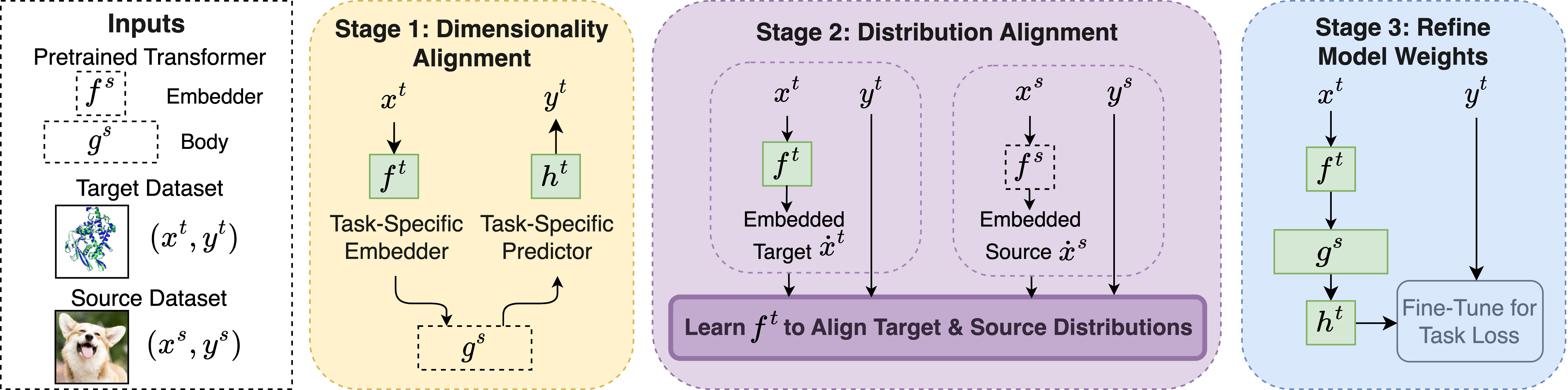
Figure 1: Orca’s three-stage fine-tuning workflow enables fast and automatic exploitation of large-scale pretrained models for solving diverse tasks. In stage 1, given target data $(x^{t},y^{t})$ and a pretrained transformer body $g^{s}$, Orca constructs an embedder architecture $f^{t}$ to map the input to the dimensionality of $g^{s}$, and a predictor architecture $h^{t}$ to convert the output of $g^{s}$ to the target output, e.g., classification logits. The weights of $f_{t}$ and $h_{t}$ are randomly initialized. In stage 2, Orca learns $f^{t}$ by minimizing the distributional distance between the embedded target features and some in-modality source features. In stage 3, Orca fine-tunes $f^{t}$, $g^{s}$, and $h^{t}$ to minimize the task loss.

The rise of large-scale pretrained models has been a hallmark of machine learning (ML) research in the past few years. Using transfer learning, these models can apply what they have learned from large amounts of unlabeled data to downstream tasks and perform remarkably well in a number of modalities, such as language, vision, and speech processing (e.g., Radford & Narasimhan, 2018; Carion et al., 2020; Baevski et al., 2020). Existing research focuses on in-modality transfer within these well-studied areas—for example, BERT models (Devlin et al., 2019) are typically only adapted for text-based tasks, and vision transformers (Dosovitskiy et al., 2021) only for image datasets.

But imagine if we could use pretrained BERT models to tackle genomics tasks, or vision transformers to solve PDEs? Effective cross-modal fine-tuning could have immense impact on less-studied areas, such as physical and life sciences, healthcare, and finance. Indeed, designing specialized networks in these areas is challenging, as it requires both domain knowledge and ML expertise. Automated machine learning (AutoML) (e.g., Roberts et al., 2021; Shen et al., 2022) and general-purpose architectures (e.g., Jaegle et al., 2022) can be used to simplify this process, but they still require training models from scratch, which is difficult for data-scarce modalities. Applying models pretrained in data-rich modalities to these new problems can potentially alleviate the modeling and data concerns, reducing the human effort needed to develop high-quality task-specific models.

Despite the potential impact, the general feasibility of cross-modal fine-tuning remains an open question. While recent work has demonstrated its possibility by applying pretrained language models to vision tasks (Dinh et al., 2022; Lu et al., 2022), referential games (Li et al., 2020c), and reinforcement learning (Reid et al., 2022), many of these approaches are ad-hoc, relying on manual prompt engineering or architecture add-ons to solve specific tasks. Besides, they often do not yield models that are competitive with those trained from scratch. We aim to tackle both of these shortcomings.

In this work, we propose a fine-tuning workflow called Orca that bridges the gap between generality and effectiveness in cross-modal learning. Our key insight is to perform task-specific data alignment prior to task-agnostic fine-tuning. By matching the data distribution of an unfamiliar modality with that of a familiar one, Orca can prevent the distortion of the pretrained weights and exploit the knowledge encoded in the pretrained models, achieving significantly better results than naive fine-tuning and state-of-the-art performance on 3 benchmarks—NAS-Bench-360 (Tu et al., 2022), PDEBench (Takamoto et al., 2022), and OpenML-CC18 (Vanschoren et al., 2014)—which contain over 60 datasets from 12 distinct data modalities.

Concretely, Orca adapts any pretrained transformer model to a downstream task via a three-stage workflow (Figure 1). First, Orca generates a task-specific embedding network architecture that maps the target inputs to sequence features which can be processed by the transformer layers (dimensionality alignment). Then, the embedding network is trained to minimize the distributional distance between the embedded target features and the features of an in-modality reference dataset (distribution alignment). Finally, the entire target model is fine-tuned to calibrate the weights with the task goal. In Section 3.4, we evaluate several standard distance metrics for distribution alignment and find that the optimal transport dataset distance (Alvarez-Melis & Fusi, 2020) attains the best empirical performance, possibly by taking the label distribution and clustering structure of the data into consideration. Thus, we use it in our subsequent experiments.

We validate Orca’s effectiveness along three axes: breadth, depth, and comparison with existing work. Breadthwise, we evaluate Orca on NAS-Bench-360 (Tu et al., 2022), an AutoML benchmark that includes 10 tasks with diverse input dimensions (1D and 2D), prediction types (point and dense), and modalities (vision, audio, electrocardiogram, physics, protein, genomics, and cosmic-ray). The empirical results, combined with our analysis, show the following:

• Cross-modal fine-tuning is promising: Orca outperforms various hand-designed models, AutoML methods, and general-purpose architectures, ranking first on 7 tasks and in the top three on all tasks. We also observe Orca’s effectiveness in a simulated limited-data setting.

• Alignment is crucial: We find an empirical correlation between alignment quality and downstream accuracy. The fact that Orca significantly outperforms naive fine-tuning demonstrates that data alignment is important.

• Alignment can be performed efficiently: Our embedder learning time is only $\sim$10% of the fine-tuning time.

Depthwise, we study two established benchmarks in practical modalities: PDEBench for solving partial differential equations (Takamoto et al., 2022) and OpenML-CC18 for classifying tabular data (Vanschoren et al., 2014). We perform in-depth analysis to show that Orca adapts vision and language transformers to learn meaningful representations of the target tasks. It matches the performance of state-of-the-art approaches, including FNO (Li et al., 2021) for PDEBench, AutoGluon (Erickson et al., 2020) and TabPFN (Hollmann et al., 2022) for OpenML-CC18.

Finally, we compare with task-specific cross-modal methods that convert tabular data into text (Dinh et al., 2022) or images (Zhu et al., 2021) to reuse existing models. The results clearly suggest that Orca is both more effective and more general. Our code is made public at https://github.com/sjunhongshen/ORCA.

2 Related Work

Table 1: Summary of existing approaches for model development for diverse tasks.

		Task-specific	General-purpose	Supports transfer to different:
		adaptation?	workflow?	input dim?	output dim?	modality?
Task-specific	Hand-designed models	✓
learning	AutoML models	✓	✓
In-modality transfer	Unimodal DA	✓		✓
	Uni/Multimodal fine-tuning	✓		✓	✓
	General-purpose models	✓	✓	✓	✓
Cross-modal transfer	Heterogeneous DA	✓		✓		✓
	Task-specific fine-tuning	✓		✓	✓	✓
	FPT		✓	✓	✓	✓
	Orca	✓	✓	✓	✓	✓

In this section, we review several groups of related work in the areas of AutoML, in-modality transfer, and cross-modal transfer. Table 1 summarizes these groups along relevant axes, and contrasts them with Orca.

AutoML for diverse tasks is a growing research area, as evidenced by the NAS-Bench-360 benchmark (Tu et al., 2022), the 2022 AutoML Decathlon competition, and recent neural architecture search (NAS) methods that target this problem, such as AutoML-Zero (Real et al., 2020), XD (Roberts et al., 2021), and DASH (Shen et al., 2022). Unlike NAS methods which repeatedly incur the overhead of designing new architectures and train them from scratch, Orca takes a fine-tuning approach and reuses existing models in data-rich modalities. That said, given the shared underlying motivation, we use NAS-Bench-360 in our experimental evaluation and compare against state-of-the-art AutoML baselines.

Unimodal domain adaptation (DA) is a form of transductive transfer learning where the source and target tasks are the same but the domains differ (Pan & Yang, 2009; Wang & Deng, 2018). Most DA methods assume that the source and target data have the same input space and support, and are concerned with different output spaces or joint/marginal distributions. Recent work studies more general settings such as different feature spaces (heterogeneous DA) or label spaces (universal DA). Our focus on cross-modal fine-tuning goes one step further to the case where neither the input-space nor the output-space support overlaps.

Unimodal fine-tuning is a more flexible transfer approach that can be applied to downstream tasks with different label or input spaces. Pretrained models are used for in-modality fine-tuning in fields like language (e.g., Jiang et al., 2020; Aghajanyan et al., 2021), vision (e.g., Li et al., 2022; Wei et al., 2022), speech (e.g., Jiang et al., 2021; Chen et al., 2022), protein (Jumper et al., 2021), and robotics (Ahn et al., 2022). Adapter networks (He et al., 2022) have been developed to improve the performance of in-modality fine-tuning. Multimodal fine-tuning expands the applicable modalities of a single pretrained model by learning embeddings of several modalities together (e.g., Radford et al., 2021; Hu & Singh, 2021; Kim et al., 2021; Alayrac et al., 2022), but these methods still focus on adapting to in-modality tasks.

General-purpose models propose flexible architectures applicable to various tasks such as optical flow, point clouds, and reinforcement learning (Jaegle et al., 2021, 2022; Reed et al., 2023). These approaches train multitask transformers from scratch using a large body of data from different tasks. Though more versatile than unimodal models, they still focus on transferring to problems within the considered pretraining modalities. Nonetheless, the success of transformers for in-modality fine-tuning motivates us to focus on adapting transformer architectures for cross-modal tasks.

Heterogeneous DA (HDA) considers nonequivalent feature spaces between the source and target domains. While most HDA methods tackle same-modality-different-dimension transfer, e.g., between images of different resolutions, there are indeed a few works studying cross-modal text-to-image transfer (Yao et al., 2019; Li et al., 2020b). However, a crucial assumption that HDA makes is that the target and source tasks are the same. In contrast, we consider more flexible knowledge transfer between drastically different modalities with distinct tasks and label sets, such as applying Swin Transformers to solving partial differential equations or RoBERTa to classifying electrocardiograms.

Cross-modal task-specific fine-tuning is a recent line of research, with most work focusing on transferring language models to other modalities like vision (Kiela et al., 2019), referential games (Li et al., 2020c), reinforcement learning (Reid et al., 2022), and protein sequences (Vinod et al., 2023). These works provide initial evidence of the cross-modal transfer capacity of pretrained models. However, they focus on hand-tailoring to a single modality, e.g., by adding ad-hoc encoders that transform agent messages (Li et al., 2020c) or decision trajectories (Reid et al., 2022) into tokens. Even when not relying on fine-tuning, work like LIFT (Dinh et al., 2022) that attempts cross-modal learning via prompting (Liu et al., 2021a) still requires ad-hoc conversion of tasks to natural text.

Frozen Pretrained Transformers (FPT) (Lu et al., 2022) is a cross-modal fine-tuning workflow that transforms the inputs to be compatible with the pretrained models. Although FPT and Orca are both general-purpose, FPT does not account for the modality difference (no stage 2 in Figure 1), but we show this step is necessary to obtain effective predictive models and outperform existing baselines.

3 Orca Workflow

In this section, we formalize the problem setup and introduce the our workflow for adapting pretrained transformers.

Problem Setup. A domain $\mathcal{D}$ consists of a feature space $\mathcal{X}$, a label space $\mathcal{Y}$, and a joint probability distribution $P(\mathcal{X},\mathcal{Y})$. In the cross-modal setting we study, the target (end-task) domain $\mathcal{D}^{t}$ and source (pretraining) domain $\mathcal{D}^{s}$ differ not only in the feature space but also the label space and by extension have differing probability distributions, i.e., $\mathcal{X}^{t}\neq\mathcal{X}^{s}$, $\mathcal{Y}^{t}\neq\mathcal{Y}^{s}$, and $P^{t}(\mathcal{X}^{t},\mathcal{Y}^{t})\neq P^{s}(\mathcal{X}^{s},\mathcal{Y}^{s})$. This is in contrast to the transductive transfer learning setting addressed by domain adaptation, where source and target domains share the label space and end task (Pan & Yang, 2009).

Given target data $\{x_{i}^{t},y_{i}^{t}\}_{i=1}^{n^{t}}$ sampled from a joint distribution $P^{t}$ in domain $\mathcal{D}^{t}$, our goal is to learn a model $m^{t}$ that correctly maps each input $x^{t}$ to its label $y^{t}$. We are interested in achieving this using pretrained transformers. Thus, we assume access to a model $m^{s}$ pretrained with data $\{x_{i}^{s},y_{i}^{s}\}_{i=1}^{n^{s}}$ in the source domain $\mathcal{D}^{s}$. Then, given a loss function $l$, we aim to develop $m^{t}$ based on $m^{s}$ such that $\mathbb{E}_{(x^{t},y^{t})\sim P^{t}}[l(m^{t}(x^{t}),y^{t})]$ is minimized. This problem formulation does not define modality explicitly and includes both in-modal and cross-modal transfer. Given the generality of the tasks we wish to explore and the difficulty of differentiating the two settings mathematically, we rely on semantics to do so: intuitively, cross-modal data (e.g., natural images vs. PDEs) are more distinct to each other than in-modal data (e.g., photos taken in two geographical locations).

Having defined the learning problem, we now present our three-stage cross-modal fine-tuning workflow: (1) generating task-specific embedder and predictor to support diverse input-output dimensions, (2) pretraining embedder to align the source and target feature distributions, and (3) fine-tuning to minimize the target loss.

3.1 Architecture Design for Dimensionality Alignment

Applying pretrained models to a new problem usually requires addressing the problem of dimensionality mismatch. To make Orca work for different input/output dimensions, we decompose a transformer-based learner $m$ into three parts (Figure 1 stage 1): an embedder $f$ that transforms input $x$ into a sequence of features, a model body $g$ that applies a series of pretrained attention layers to the embedded features, and a predictor $h$ that generates the outputs with the desired shape. Orca uses a pretrained architecture and weights to initialize the model body $g$ but replaces $f$ and $h$ with layers designed to match the target data with the pretrained model’s embedding dimension. In the following, we describe each module in detail.

Custom Embedding Network. Denote the feature space compatible with the pretrained model as $\mathcal{\dot{X}}$. For a transformer with maximum sequence length $S$ and embedding dimension $D$, $\mathcal{\dot{X}}=\mathbb{R}^{S\times D}$. The target embedder $f^{t}:\mathcal{X}\rightarrow\mathcal{\dot{X}}$ is designed to take in a tensor of arbitrary dimension from $\mathcal{X}$ and transform it to $\mathcal{\dot{X}}$. In Orca, $f^{t}$ is composed of a convolutional layer with input channel $c_{in}$, output channel $c_{out}$, kernel size $k$, and stride $k$, generalizing the patching operations used in vision transformers to 1D and higher-dimensional cases. We set $c_{in}$ to the input channel of $x$ and $c_{out}$ to the embedding dimension $D$. We can either treat $k$ as a hyperparameter or set it to the smallest value for which the product of output shape excluding the channel dimension $\leq S$ to take full advantage of the representation power of the pretrained model. In the latter case, when we flatten the non-channel dimensions of the output tensors after the convolution, pad and then transpose it, we can obtain sequence features with shape $S\times D$. Finally, we add a layer norm and a positional embedding to obtain $\dot{x}$.

Pretrained Transformer Body. The model body $g$ takes the embedding $\dot{x}\in\mathcal{\dot{X}}$ as input and outputs features $\dot{y}\in\mathcal{\dot{Y}}$; the dot is used to differentiate these intermediate representations from the raw inputs and labels. For transformer-based $g$, both the input and output feature spaces $\mathcal{\dot{X}},\mathcal{\dot{Y}}$ are $\mathbb{R}^{S\times D}$.

Custom Prediction Head. Finally, the target model’s prediction head $h^{t}$ must take $\dot{y}\in\mathcal{\dot{Y}}$ as input and return a task-dependent output tensor. Different tasks often specify different types of outputs, e.g., classification logits in $\mathbb{R}^{K}$, where $K$ is the number of classes, or dense maps where the spatial dimension is the same as the input and per index logits correspond to $K$ classes. Thus, it is crucial to define task-specific output modules and fine-tune them for new problems. In Orca, we use the simplest instantiation of the predictors. For classification, we apply average pooling along the sequence length dimension to obtain 1D tensors with length $D$ and then use a linear layer that maps $D$ to $K$. For dense prediction, we apply a linear layer to the sequence outputs so the resulting tensor has shape $(S,k^{\mathrm{ndim}(\mathcal{Y})}K)$, where $k^{\mathrm{ndim}(\mathcal{Y})}$ is the downsampling factor of the embedder convolution kernel with stride $k$. This upsamples by the same factor that the embedder downsampled. Then, we can mold the tensor to the desired output dimension.

With an architecture based on the pretrained model but also compatible with the target task, we can now turn our attention to data alignment for better adaptation.

Table 2: Prediction errors ($\downarrow$) on 10 diverse tasks. “NAS-Bench-360” refers to the task-wise best of all AutoML baselines evaluated in the paper, including DARTS (Liu et al., 2019b), DenseNAS (Fang et al., 2020), and 4 others. “FPT” refers to fine-tuning the layer norms of RoBERTa/Swin. On 7/10 problems, Orca ranks the first among all competitors. See Appendix A.4.2 for the error bars.

	CIFAR-100	Spherical	Darcy Flow	PSICOV	Cosmic	NinaPro	FSD50K	ECG	Satellite	DeepSEA
	0-1 error (%)	0-1 error (%)	relative $\ell_{2}$	MAE8	1-AUROC	0-1 error (%)	1- mAP	1 - F1 score	0-1 error (%)	1- AUROC
Hand-designed	19.39	67.41	8E-3	3.35	0.127	8.73	0.62	0.28	19.80	0.30
NAS-Bench-360	23.39	48.23	2.6E-2	2.94	0.229	7.34	0.60	0.34	12.51	0.32
DASH	24.37	71.28	7.9E-3	3.30	0.19	6.60	0.60	0.32	12.28	0.28
Perceiver IO	70.04	82.57	2.4E-2	8.06	0.485	22.22	0.72	0.66	15.93	0.38
FPT	10.11	76.38	2.1E-2	4.66	0.233	15.69	0.67	0.50	20.83	0.37
Orca	6.53	29.85	7.28E-3	1.91	0.152	7.54	0.56	0.28	11.59	0.29

3.2 Embedder Learning for Distribution Alignment

Intuitively, transferring knowledge across similar modalities should be easier than across distant ones. Hence, given a target task in a new modality, we aim to manipulate the target data so that they become closer to the pretraining modality. One way to achieve this is to train the embedder before actually fine-tuning the model body in a way that makes the embedded target features resemble the source features which the pretrained model body is known to perform well on.

Formally, let $f^{s}:\mathcal{X}^{s}\to\mathcal{\dot{X}}$ denote the pretrained source embedder (the part of $m^{s}$ that transforms the raw data to sequence features) and $f^{t}$ the randomly initialized target embedder discussed in the previous section. We can learn $f^{t}$ to minimize the distance between the joint distribution of the target embeddings $\big{(}f^{t}(x^{t}),y^{t}\big{)}$ and that of the source embeddings $\big{(}f^{s}(x^{s}),y^{s}\big{)}$. There are many metrics for measuring this distributional distance. To understand whether they affect adaptation differently, we perform a preliminary study in Section 3.4 on three representatives.

3.3 Weight Refining for Downstream Adaptation

After training the embedder, we perform full fine-tuning by updating all model parameters to minimize the target loss. This step further aligns the embedder and predictor with the pretrained model. In Section 4.1, we compare Orca with standard fine-tuning without data alignment and show that our approach improves performance while reducing variance. There are orthogonal works that study how to best fine-tune a model (e.g., Liu et al., 2022; He et al., 2022). We compare with one strategy used in FPT (Lu et al., 2022) in Section 4.1 but leave further exploration for future work.

3.4 Evaluation of Distribution Alignment Metrics

We evaluate the effectiveness of three distance metrics for data alignment during embedding learning: (1) the pairwise Euclidean distance, which aligns the scales and ranges of the datasets without using any distributional information; (2) the moment-based maximum mean discrepancy (MMD) (Gretton et al., 2012), which uses the distribution of $f(x)$ to align the feature means; and (3) optimal transport dataset distance (OTDD) (Alvarez-Melis & Fusi, 2020), which uses both the feature and label distributions $\big{(}f(x),y\big{)}$ to align the high-level clustering structure of the datasets.

We substitute each metric into the Orca workflow (implementation details in Section 4) and evaluate them on 10 tasks from diverse modalities (benchmark details in Section 4.1). The aggregate performance (Figure 2) and per-task rankings (Appendix A.4.4) show that embedder learning with OTDD has the best overall results, so we use it in our subsequent experiments. We conjecture that its good performance is due to how the label information is considered during alignment.

Indeed, for both the source and target datasets, OTDD represents each class label as a distribution over the in-class features: $y\mapsto P(\mathcal{\dot{X}}|\mathcal{Y}=y)$. This transforms the source and target label sets into the shared space of distributions over $\mathcal{\dot{X}}$. Then, we can define the distance $d_{\mathcal{Y}}(y^{t},y^{s})$ between different labels using the $p$-Wasserstein distance associated with the $l_{2}$ distance $\|\dot{x}^{t}-\dot{x}^{s}\|_{2}^{2}$ in $\mathcal{\dot{X}}$, which in turn allows us to measure the distributional difference in $\mathcal{\dot{X}}\times\mathcal{Y}$:

$$d_{\mathcal{\dot{X}}\times\mathcal{Y}}\big{(}(\dot{x}^{t},y^{t}),(\dot{x}^{s},y^{s})\big{)}=\big{(}d_{\mathcal{\dot{X}}}(\dot{x}^{t},\dot{x}^{s})^{p}+d_{\mathcal{Y}}(y^{t},y^{s})^{p}\big{)}^{1/p}.$$

We refer the readers to Alvarez-Melis & Fusi (2020) for the exact formulation. Yet the implication from our experiments is that, as we learn $f^{t}$ to minimize OTDD, we are not only aligning individual data points, but also grouping features with the same label together in the embedding space, which could potentially facilitate fine-tuning.

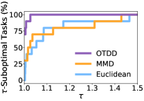
Figure 2: Performance profiles (Dolan & Moré, 2002) of Orca with different alignment metrics. Larger values (fractions of tasks on which a method is within $\tau$-factor of the best) are better. The OTDD curve being in the upper left shows it is often the best.

Despite its effectiveness for data alignment, OTDD is generally expensive to compute. In Section A.1 of the Appendix, we analyze its computational complexity and propose an efficient approximation to it using class-wise subsampling.

Before ending this section, we emphasize that our goal is not to discover the best alignment metric but to provide a general fine-tuning framework that works regardless of the metric used. Thus, we leave designing more suitable distance metrics for future work.

4 Experiments

Table 3: Prediction errors ($\downarrow$) of Orca, naive fine-tuning, and training RoBERTa/Swin from scratch. We consider adapting all parameters (full setting) vs. only the layer norms (FPT setting).Orca is better in both settings. The fact that full fine-tuning generally outperforms tuning only the layer norms is also consistent with recent observations (Rothermel et al., 2021). See Appendix A.4.3 for the error bars.

	CIFAR-100	Spherical	Darcy Flow	PSICOV	Cosmic	NinaPro	FSD50K	ECG	Satellite	DeepSEA
Train-from-scratch	50.87	76.67	8.0E-2	5.09	0.50	9.96	0.75	0.42	12.38	0.39
Fine-tuning	7.67	55.26	7.34E-3	1.92	0.17	8.35	0.63	0.44	13.86	0.51
Orca	6.53	29.85	7.28E-3	1.91	0.152	7.54	0.56	0.28	11.59	0.29
Fine-tuning (layernorm)	10.11	76.38	2.11E-2	4.66	0.233	15.69	0.67	0.50	20.83	0.37
Orca (layernorm)	7.99	42.45	2.21E-2	4.97	0.227	15.99	0.64	0.47	20.54	0.36

Having introduced how Orca tackles cross-modal fine-tuning, we proceed with showing its empirical efficacy via three thematic groups of experiments: (1) we evaluate Orca across a breadth of modalities and show that it outperforms hand-designed, AutoML-searched, and general-purpose architectures; we study its key components to understand the mechanism behind cross-modal fine-tuning and exemplify how it benefits limited-data modalities; (2) we perform in-depth analyses in two modalities, PDE solving and tabular classification, to show that Orca is competitive with expert-designed task-specific models; (3) we compare Orca with previous ad-hoc cross-modal learning techniques to show that we strike a balance between generality and effectiveness.

Experiment Protocol. While our workflow accepts a wide range of pretrained transformers as model bodies, we use RoBERTa (Liu et al., 2019c) and Swin Transformers (Liu et al., 2021b), which are representatives of the most studied language and vision modalities, to exemplify Orca’s efficacy. We implement the base models using the Hugging Face library (Wolf et al., 2019) and choose CoNLL-2003 and CIFAR-10 as the proxy datasets, respectively. For each task, we first perform hyperparameter tuning in the standard fine-tuning setting to identify the optimal target sequence length, batch size, and optimizer configuration. Experiments are performed on a single NVIDIA V100 GPU and managed using the Determined AI platform. Results are averaged over 5 trails. For other details, see Appendix A.2.

4.1 A Breadth Perspective: Can Pretrained Models Transfer Across Modalities?

In this section, we highlight the most important observation of this work: cross-modal fine-tuning with data alignment can solve diverse tasks effectively and efficiently. To show this, we test Orca on 10 tasks from NAS-Bench-360 covering diverse 1D/2D problems such as protein folding, cardiac disease prediction, and cosmic-ray detection. Following Table 1, we consider 3 classes of baselines: (1) hand-designed, task-specific models identified by Tu et al. (2022); (2) general-purpose models represented by Perceiver IO (Jaegle et al., 2022); (3) AutoML methods, including the leading algorithm on NAS-Bench-360, DASH (Shen et al., 2022).

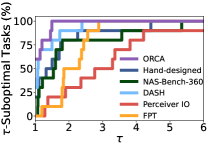
Figure 3: Aggregating Table 2 results using performance profiles (Dolan & Moré, 2002). Larger values (fractions of tasks on which a method is within $\tau$-factor of the best) are better. Orca being in the top left corner means it is often the best.

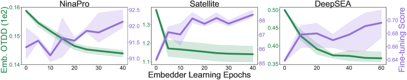
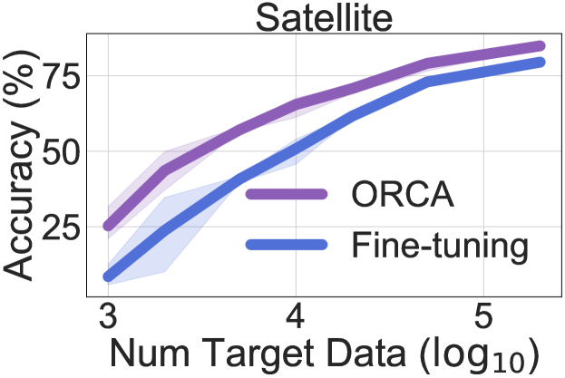
Figure 4: Left: Final accuracy and embedding distribution distance vs. embedder learning epochs on three NAS-Bench-360 tasks. As we learn to map the target data to the source modality better (smaller OTDD), we obtain models with better downstream performance. This shows an empirical correlation between fine-tuning accuracy and alignment quality. Right: Accuracy ($\uparrow$) of Orca vs. naive fine-tuning with varying dataset size on task Satellite. Orca has higher performance gains in low-data regime.

We report the prediction error for each method on each task in Table 2 and visualize the aggregate performance in Figure 3. Orca achieves the lowest error rates on 7 of 10 tasks and the best aggregate performance. Specifically, it outperforms hand-designed architectures on all tasks. It beats all AutoML baselines on all tasks except DeepSEA and NinaPro, where it ranks second and third, respectively. The improvements from the embedder learning stage of Orca come at a small computational overhead—Table 11 in the Appendix shows that the time needed for data alignment is only a small portion (11%) of the fine-tuning time.

Our results validate the finding in prior cross-modal work that pretrained transformers learn knowledge transferable to seemingly unrelated tasks. In the following, we dissect the success of Orca via multiple ablations and identify 3 factors crucial to exploiting the learned knowledge: data alignment, full fine-tuning, pretraining modality selection.

Key 1: Aligning Feature Distributions

To understand whether the good performance of Orca is indeed attributed to the data alignment process, which is our key innovation, we compare it with naive fine-tuning that does not align the data (Table 3, middle rows). We see that Orca consistently outperforms naive fine-tuning. Moreover, we show in Appendix A.4.4 that Orca with different alignment metrics all obtain better performance than fine-tuning. Thus, closing the gap between the target and pretraining modalities can facilitate model adaptation.

To further isolate the impact of data alignment, we compare Orca with a train-from-scratch baseline (Table 3, first row) which trains RoBERTa and Swin using only the target data. We observe training from scratch is worse than Orca but better than fine-tuning on ECG, Satellite, and DeepSea. We conjecture that this is because when the target modality differs significantly from the pretraining modality, naive fine-tuning may harm transfer, but aligning the feature distribution using Orca can resolve this issue and benefit transfer. Indeed, recent work has shown that optimizing directly for the task loss may distort the pretrained weights and lead to suboptimal solutions (Kumar et al., 2022; Lee et al., 2022). By manipulating the target distribution to look like the source distribution, we lower the risk of weight distortion, thus obtaining better downstream performance.

We also quantify the effect of data alignment by training the embedder for different number of epochs and see whether optimizing distribution distance to various levels of convergence affects downstream performance. Figure 4 (left) plots the fine-tuning accuracy and the final distribution distance for different embedder learning levels. We see that as the dataset distance decreases, the fine-tuning accuracy increases. In addition, learning the embedder separately from fine-tuning stabilizes training, as the performance variance of Orca is constantly lower than that of naive fine-tuning. These results confirm that data alignment is the key to effective cross-modal fine-tuning.

Key 2: Fine-Tuning All Model Parameters

As discussed in Section 2, Frozen Pretrained Transformers (FPT) (Lu et al., 2022) is a related work that showed pretrained language models contain knowledge relevant to out-of-modality tasks. While FPT presented a general pipeline for adapting GPT-2 to tasks like CIFAR-10, the resulting models were not as good as those trained from scratch. FPT differs from Orca in that (1) it does not perform data alignment, and (2) it only fine-tunes the layer norms. We have verified the importance of (1). Now, we isolate the impact of (2) by fine-tuning only the layer norms for Orca.

The bottom rows of Table 3 show that Orca with fine-tuning the layer norms outperforms FPT, so pretraining the embedder can boost the performance of FPT. However, this performance gain is smaller than that in the full fine-tuning setting, which implies that full fine-tuning can take better advantage of the learned embeddings. In terms of runtime, FPT yields less than a 2$\times$ speedup compared with full fine-tuning (Appendix A.4.6), despite the fact that we are updating many fewer parameters. This is unsurprising since gradients are still back-propagated through the entire network. Therefore, when computation allows, we recommend using Orca with full fine-tuning for better performance.

Key 3: Adapting From the Right Modality

Finally, we study how the pretraining modality affects fine-tuning. In the results reported so far, we choose pretrained models for each task based on the input dimension, i.e., we use RoBERTa for all 1D tasks and Swin for all 2D tasks. Now, we evaluate the opposite approach, focusing on two tasks: DeepSEA (1D) and Spherical (2D). This evaluation is straightforward to perform by switching the model bodies, since the embedder architecture of Orca handles all input transformations needed to obtain the sequence features. The results are shown in Table 13 in the Appendix. We see that fine-tuned RoBERTa outperforms Swin on the 1D task, possibly because the DeepSEA data (genomics sequences) are structured more like language than images with discrete units of information and general grammatical rules. More crucially, for both tasks, models with smaller final OTDDs have better fine-tuning accuracy. This suggests a way of selecting pretrained models by comparing the optimized OTDDs and picking the one with the smallest value.

Apart from these three key insights, recall that one of our motivations for cross-modal fine-tuning is to help tasks with limited data, where training models from scratch is difficult. Indeed, for vanilla fine-tuning, a small amount of data may not give enough signal to update the pretrained weights, but it is possible to learn a good embedder first with Orca, which can then make fine-tuning easier. In Figure 4 (right), we vary the dataset size and find that the performance gain of Orca increases as the dataset size decreases. Meanwhile, using Orca allows us to match the performance of naive fine-tuning on 3$\times$ amount of data. Thus, it can benefit model development in domains where data collection is costly. Beyond the cross-modal setting, we also verify Orca’s efficacy for in-modality transfer in Appendix A.8.1.

4.2 A Depth Perspective: Cross-Modal Fine-Tuning for PDE and Tabular Tasks

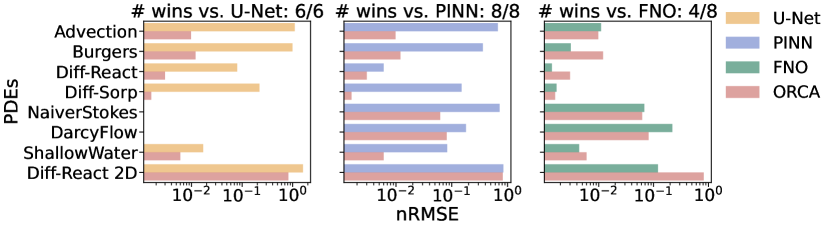
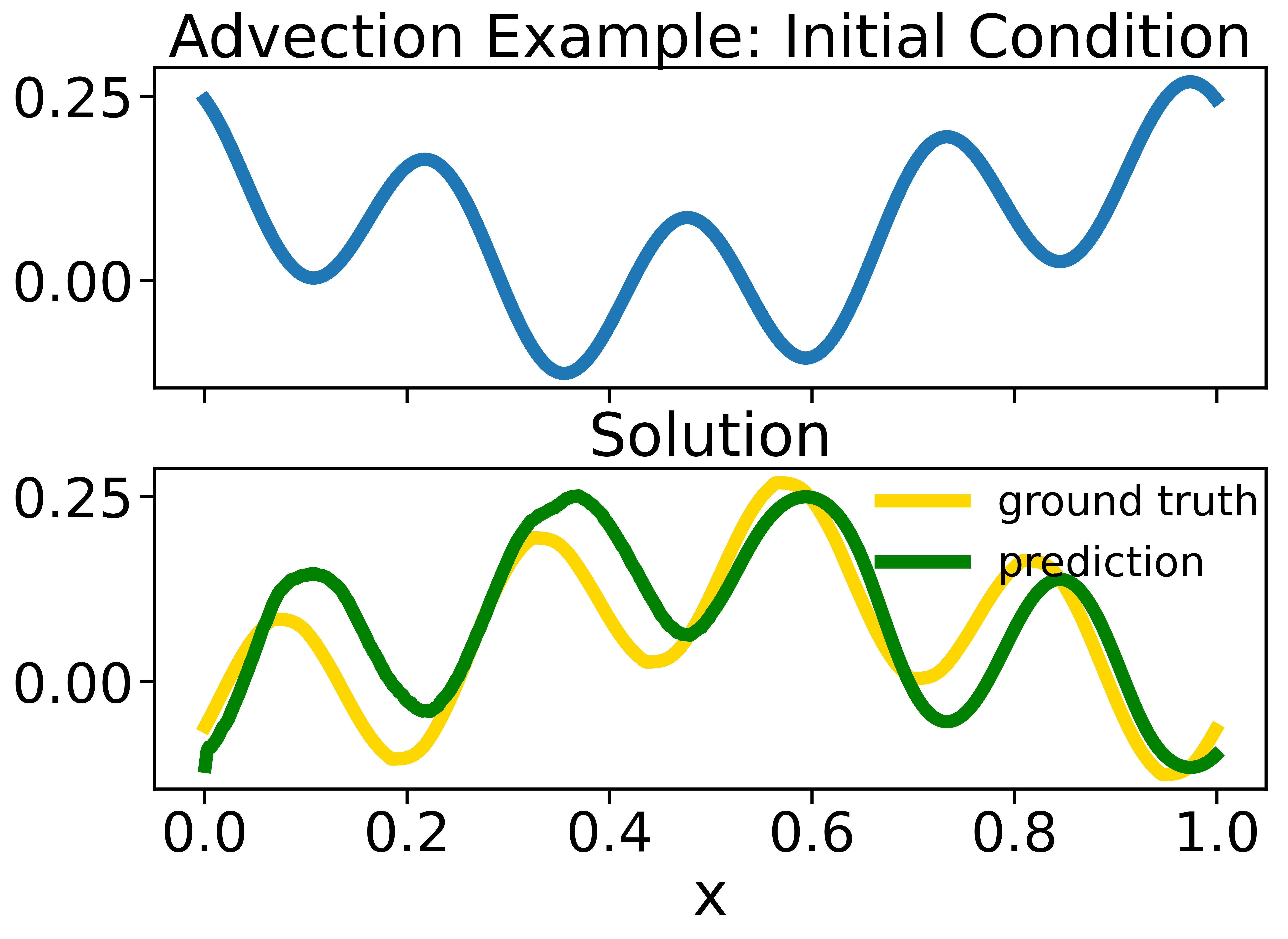
Figure 5: Left: Normalized Root Mean Squared Errors (nRMSEs, $\downarrow$) for Orca vs. baselines on 8 PDEBench tasks with varying dimensions (1D/2D). We only evaluate datasets that can fit into a single V100 GPU. Overall, Orca is much better than U-Net and PINN and on par with FNO. For detailed numerical results, see Table 14 in the Appendix. Right: Orca is trained on resolution 256 and directly evaluated on resolution 512. The prediction still matches the ground truth.

After validating Orca on a broad set of tasks, we dive into two specific modalities, PDE solving and tabular classification, to show that cross-modal fine-tuning is promising for model development in highly specialized areas. Orca can not only achieve high prediction accuracy in both domains, but also recover an important property of Neural Operators—modeling PDEs with zero-shot super-resolution.

PDEBench for Scientific ML

ML models for physical systems have gained increasing interest in recent years. To study how cross-modal fine-tuning can help in the scientific ML context, we evaluate Orca on 8 datasets from PDEBench (Takamoto et al., 2022) and compare against state-of-the-art task-specific models: the physics-informed neural network PINN (Raissi et al., 2019), Fourier neural operator (FNO) (Li et al., 2021), and the generic image-to-image regression model U-Net (Ronneberger et al., 2015). We focus on the forward prediction problems. See Appendix A.5 for the experiment details.

As shown in Figure 5 (left), Orca outperforms PINN and U-Net on all evaluated datasets and beats FNO on half of them, using a smaller training time budget than U-Net and FNO. This is an impressive result given that the baselines, in particular FNO, are carefully designed with domain knowledge. More crucially, as shown in Figure 5 (right), Orca achieves zero-shot super-resolution (trained on a lower resolution and directly evaluated on a higher resolution) when using the RoBERTa backbone and an embedder with pointwise convolutions. This generalization ability has only been observed in FNOs. Orca also achieves it possibly because the sequence features generated by pointwise convolutions are resolution-invariant and can capture the intrinsic flow dynamics. These results demonstrate the potential of cross-modal fine-tuning in the scientific ML context.

Table 4: Tabular results with baselines from Hollmann et al. (2022) and Dinh et al. (2022). “Diff. from XGBoost” is the across-task average of per-task difference from XGBoost. Orca beats classical approaches and advanced transformer methods on 19 tasks. For per-task results, see Appendix A.6.

OpenML-CC18	LightGBM	CatBoost	XGBoost	AutoGluon	TabPFN	Orca
# Wins/Ties	1/30	1/30	3/30	12/30	7/30	12/30
Avg. AUROC ($\uparrow$)	0.884	0.8898	0.8909	0.8947	0.8943	0.8946
Diff. from XGBoost	-6.97E-3	-1.18E-3	0	+3.74E-3	+3.38E-3	+3.63E-3

LIFT Tasks	LogisticRegression	SVM	XGBoost	LIFT GPT-3	Orca
# Wins/Ties	2/14	3/14	2/14	2/14	7/14
Avg. Acc. ($\uparrow$)	79.58	80.63	78.21	79.63	83.80
Diff. from XGBoost	+1.37	+2.42	0	+1.42	+5.60

OpenML for Tabular Classification

Despite being one of the most commonly seen data types, tabular data are still primarily modeled with classical ML methods like XGBoost (Chen & Guestrin, 2016). More recently, deep learning approaches such as AutoGluon (Erickson et al., 2020) and TabPFN (Hollmann et al., 2022) have applied task-specific transformers to tabular data with some success. We next show that Orca can adapt pretrained RoBERTa to tabular data, outperforming classical methods and matching the performance of recent deep learning approaches.

Similar to Hollmann et al. (2022), we evaluate Orca on 30 datasets from the OpenML-CC18 benchmark (Vanschoren et al., 2014), comparing against both classical boosting algorithms (Ke et al., 2017; Ostroumova et al., 2017) and advanced transformer-based models (Erickson et al., 2020; Hollmann et al., 2022). As shown in Table 4 (top), Orca ranks first on 12/30 tasks and works as well as AutoGluon, the state-of-the-art AutoML method on tabular data. It also outperforms TabPFN (Hollmann et al., 2022), a transformer-based prior-data fitted network, on 16/30 tasks.

It is worth noting that no single method performs best on all tasks. For datasets where there are limited data described by categorical variables (e.g., dresses-sales), boosting algorithms perform poorly, but Orca does significantly better. For datasets with balanced labels and consisting of a few numerical variables (e.g., diabetes), classical methods are sufficient and less prone to overfitting than large models. Nonetheless, our results confirm again that cross-modal fine-tuning can be appealing for tackling real-life problems.

4.3 Comparison with Task-Specific Cross-Modal Work

As stated in the introduction, one motivation of Orca is that the handful of existing cross-modal methods are mostly ad-hoc and tailored to specific modalities. Developing them thus requires a thorough understanding of the target data. To show that Orca performs better while being generally applicable to arbitrary domains, we compare with (1) IGTD (Zhu et al., 2021), which converts gene-drug features to images and applies CNNs to predict drug response; and (2) LIFT (Dinh et al., 2022), which transforms tabular data into text to prompt a pretrained GPT-3. Table 5 shows the $R^{2}$ score for the drug response tasks, and Table 4 (bottom) shows the classification accuracy for LIFT datasets. Once again, Orca beats these carefully curated task-specific methods, proving itself as both general and highly effective.

Table 5: Coefficient of determination ($R^{2}$, $\uparrow$) on two drug response prediction datasets. Orca outperforms IGTD, which converts raw tabular features to images to apply vision models.

$R^{2}$	Dataset 1: CTRP	Dataset 2: GDSC
IGTD-CNN	0.856$\pm$0.003	0.74$\pm$0.006
Orca	0.86$\pm$0.002	0.831$\pm$0.002

4.4 Limitation and Future Work

We identify several future directions based on our experiment results. First, it is worth studying the effect of pretraining modality further and develop a systematic way of selecting pretrained models. Then, we can incorporate model selection into Orca for a more automated pipeline. Second, while Orca leverages the simplest fine-tuning paradigm, it is possible to combine it with more sophisticated transfer techniques such as adapters (He et al., 2022). We briefly study how prompting (Bahng et al., 2022; Jia et al., 2022) can be applied to diverse tasks in Appendix A.8.2 and find that it is less effective for out-of-modality problems, but we might boost its performance using Orca. Lastly, we currently evaluate Orca on 1D/2D tasks. It is also important to validate it on more settings, such as high-dimensional problems and reinforcement learning (Reid et al., 2022).

5 Conclusion

In this paper, we study how we can reuse existing models for new and less-explored areas. We propose a novel and effective cross-modal fine-tuning framework, Orca, that aligns the end-task data from an arbitrary modality with a model’s pretraining modality to improve fine-tuning performance. Our work not only signals the potential of large-scale pretraining for diverse tasks but also lays out a path for a largely uncharted data-centric paradigm in ML.

Appendix A Appendix

A.1 Embedding Learning with Optimal Transport Dataset Distance

A.1.1 Literature Review

Due to the limited space, we do not give a full review of the optimal transport dataset distance (OTDD) (Alvarez-Melis & Fusi, 2020) in the main text. Here, we briefly recall the optimal transport (OT) distance and explain OTDD in detail.

Consider a complete and separable metric space $\mathcal{X}$ and let $\mathcal{P}(\mathcal{X})$ be the set of probability measures on $\mathcal{X}$. For $\alpha,\beta\in\mathcal{P}(\mathcal{X})$, let $\Pi(\alpha,\beta)$ be the set of joint probability distributions on $\mathcal{X}\times\mathcal{X}$ with marginals $\alpha$ and $\beta$ in the first and second dimensions respectively. Then given a cost function $c(\cdot,\cdot):\mathcal{X}\times\mathcal{X}\rightarrow\mathbb{R}^{+}$, the classic OT distance with cost $c$ is defined by:

$$\text{OT}_{c}(\alpha,\beta):=\min_{\pi\in\Pi(\alpha,\beta)}\int_{\mathcal{X}\times\mathcal{X}}c(x,y)d\pi(x,y).$$ (1)

When $\mathcal{X}$ is equipped with a metric $d_{\mathcal{X}}$, we can use $c(x,y)=d_{X}(x,y)^{p}$ for some $p\geq 1$ and obtain the $p$-Wasserstein distance, $W_{p}(\alpha,\beta):=(\text{OT}_{d_{\mathcal{X}}^{p}}(\alpha,\beta))^{\frac{1}{p}}$.

Now consider the case of finite datasets with features in $\mathcal{X}$ and labels in a finite set $\mathcal{Y}$. Each dataset can be considered a discrete distribution in $\mathcal{P}(\mathcal{X}\times\mathcal{Y})$. To define a distance between datasets, a natural approach is to define an appropriate cost function on $\mathcal{Z}:=\mathcal{X}\times\mathcal{Y}$ and consider the optimal transport distance. Indeed, for any metric $d_{\mathcal{Y}}$ on $\mathcal{Y}$ and any $p\geq 1$, $\mathcal{Z}$ can be made a complete and separable metric space with metric

$$d_{\mathcal{Z}}((x,y),(x^{\prime},y^{\prime}))=(d_{\mathcal{X}}(x,x^{\prime})^{p}+d_{\mathcal{Y}}(y,y^{\prime})^{p})^{\frac{1}{p}}$$ (2)

It is usually not clear how to define a natural distance metric in $\mathcal{Y}$, so instead we proceed by representing each class $y\in\mathcal{Y}$ by $P(\mathcal{X}|\mathcal{Y}=y)$, the conditional distribution of features $\mathcal{X}$ given $\mathcal{Y}=y$. More specifically, for a dataset $\mathcal{D}\in\mathcal{P}(\mathcal{X}\times\mathcal{Y})$, denote this map from classes to conditional distributions by $F(\mathcal{D},\cdot):\mathcal{Y}\to\mathcal{P}(\mathcal{X})$. Then we can transform any dataset over $\mathcal{X}\times\mathcal{Y}$ into one over $\mathcal{X}\times\mathcal{P}(\mathcal{X})$ via $G(\mathcal{D}):=(\text{proj}_{\mathcal{X}},F(\mathcal{D},\text{proj}_{Y}))$.

As discussed above, $W_{p}$ is a natural notion of distance in $\mathcal{P}(\mathcal{X})$, so by substituting $\mathcal{Y}\mapsto\mathcal{P}(\mathcal{X})$ and $d_{\mathcal{Y}}\mapsto W_{p}$ in Equation 2, we can define the ($p$-)optimal transport dataset distance between datasets $\mathcal{D}_{A}$ and $\mathcal{D}_{B}$ by

$$\text{OTDD}(\mathcal{D}_{A},\mathcal{D}_{B}):=\text{OT}_{(d_{\mathcal{X}}^{p}\times W_{p}^{p})^{\frac{1}{p}}}(G(\mathcal{D}_{A}),G(\mathcal{D}_{B}))$$ (3)

A.1.2 Computational considerations

As we aim for a practical fine-tuning workflow, computational cost is a crucial concern. While Alvarez-Melis & Fusi (2020) proposed two variants of OTDD—the exact one and a Gaussian approximation, we observe from our experiments that optimizing the exact OTDD leads to better performance. In the following, we will focus on analyzing the computational cost of the exact OTDD.

Given datasets with $D$-dimensional feature vectors, estimating vanilla OT distances can be computationally expensive and has a worst-case complexity of $O(D^{3}\log D)$ (Pele & Werman, 2009). However, adding an entropy regularization term $\epsilon H(\pi|\alpha\otimes\beta)$ to Equation 1, where $H$ is the relative entropy and $\epsilon$ controls the time-accuracy trade-off, can be solved efficiently with the Sinkhorn algorithm (Cuturi, 2013). This reduces OT’s empirical complexity to $O(D^{2})$ and makes the time cost for computing OTDD manageable for Orca’s workflow.

Algorithm 1 Efficient approximation of OTDD using class-wise subsampling.

  Input: target dataset $\{x^{t},y^{t}\}$, number of target classes $K^{t}$, source dataset $S=\{x^{s},y^{s}\}$, subsample size $b$, subsample round $R$

  for each class $i\in[K^{t}]$ in the target dataset do

     Compute class weight $w_{i}=\frac{\text{number of target data in class }i}{\text{total number of target data}}$

     Generate data loader $D_{i}$ consisting of data in class $i$

  end for

  for $i\in[K^{t}]$ do

     for $r\in[R]$ do

        Subsample $b$ target data points $D_{ir}$ uniformly at random from $D_{i}$

        Compute class-wise distance $d_{ir}=OTDD(D_{ir},S)$

     end for

     Approximate class-wise OTDD by $d_{i}=\frac{1}{R}\sum_{i=1}^{R}d_{ir}$

  end for

  Approximate OTDD by $d=\sum_{i=1}^{K^{t}}w_{i}\cdot d_{i}$

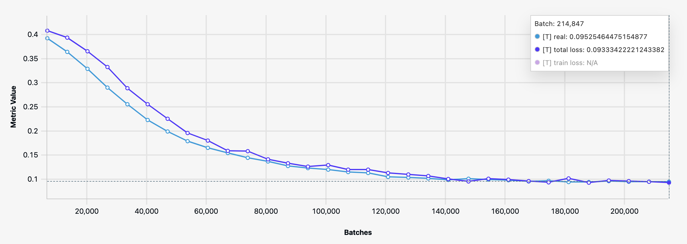
Figure 6: Screenshot of OTDD curves during embedding learning in one task. x-axis is the number of optimization steps, y-axis represents OTDD (1E2). We use Algorithm 1 to approximate the exact OTDD as the loss function for optimization on GPU (purple curve). We also track the actual OTDD on CPU (blue curve). We can see that the proposed algorithm works well, which allows us to perform embedding learning efficiently.

During implementation of Orca, we also observed memory issues for computing OTDD using the entire target and source datasets on GPUs. To alleviate this, we reduce the dimensionality of the feature vectors by taking the average along the sequence length dimension. We further propose a class-wise subsampling strategy for approximating OTDD on GPUs (Algorithm 1). In short, we split the $K$-class target dataset into $K$ datasets based on the labels and compute the class-wise OTDD between each single-class target dataset and the entire source dataset. Each class-wise OTDD can be approximated with the average of batch samples similar to how stochastic gradient descent approximates gradient descent. After that, we approximate the OTDD between the target and source datasets using the weighted sum of the $K$ class-wise OTDDs. To verify that the approximation works empirically, we track the approximated OTDD (computed on GPUs) and the actual OTDD (computed on CPUs) and visualize the loss curves during Orca’s embedder learning process (Figure 6). We can see that the estimated value adheres to the actual value.

Leveraging both the Sinkhorn algorithm and class-wise approximation, the embedder learning process only takes up a small fraction of the total fine-tuning time in practice, as shown in Table 11 in the later experiment results section. Hence, we invest a reasonable time budget but achieve significantly improved cross-domain transfer performance using Orca.

A.2 Orca Implementation

A.2.1 Pretrained Models

We evaluated Orca with two pretrained models in our experiments. In Table 2, for all 2D tasks including CIFAR-100, Spherical, Darcy Flow, PSICOV, Cosmic, NinaPro, and FSD50K, we use the following model. As Swin has a pretrained resolution, we reshape the inputs for our tasks to the resolution before feeding them into the model.

Name	Pretrain	Resolution	Num Params	FLOPS	FPS
Swin-base (Liu et al., 2021b)	ImageNet-22K	224$\times$224	88M	15.4G	278

For all 1D tasks including ECG, Satellite, DeepSEA, JSB Chorales, ListOps,and Homology, we use the following model:

Name	Pretrain	Num Params	FLOPS
RoBERTa-base (Liu et al., 2019c)	Five English-language corpora	125M	1.64E20

We use the Hugging Face transformers library (Wolf et al., 2019) to implement the pretrained models.

A.2.2 Hyperparameter Tuning

As Orca is both task-agnostic and model-agnostic, it can be applied to fine-tuning a variety of pretrained transformers on drastically different end tasks with distinct datasets. Hence, it is hard to define one set of fine-tuning hyperparameters for all (model, task) pairs. At the same time, optimizing large-scale pretrained transformers can be challenging due to their large model sizes, as the downstream performance depends largely on the hyperparameters used. For instance, using a large learning rate can distort pretrained weights and lead to catastrophic forgetting. Therefore, in our experiments, given a (model, task) pair, we first apply hyperparameter tuning using the Asynchronous Successive Halving Algorithm (ASHA) (Li et al., 2020a) to the standard fine-tuning setting (i.e., after initializing the embedder and predictor architectures, directly updating all model weights to minimize the task loss) to identify a proper training configuration. Then, we use the same set of hyperparameters found for all our experiments for the particular (model, task) combination. Note that even though we did not explicitly state this in the main text, the hyperparameter tuning stage can be directly integrated into the Orca workflow between stage 1 and stage 2. In this sense, Orca is still an automated cross-modal transfer workflow that works for diverse tasks and different pretrained models.

The configuration space for ASHA can be customized for each task. In general, the following search space is sufficient:

• Target sequence length: 8, 64, 512 for RoBERTa

• Batch size: 4, 16, 64

• Gradient clipping: -1, 1

• Dropout: 0, 0.05

• Optimizer: SGD, Adam, AdamW

• Learning rate: 1E-2, 1E-3, 1E-4, 1E-5

• Weight decay: 0, 1E-2, 1E-4

A.2.3 More Details on Embedder Architecture Design

In the current workflow, we use the following procedure to determine the kernel size $k$ for the embedder’s convolution layer:

• For RoBERTa: we apply hyperparameter search to the vanilla fine-tuning baseline to find the optimal sequence length $s^{*}$ for the second dimension of the embedder output with shape $(batch\_size,seq\_len,embed\_dim)$. The configuration space is $\{8,64,512\}$. Then, $k$ is set to largest value such that after applying convolution with $c_{out}=embed\_dim$ (e.g., $768$ for RoBERTa) and transposing the last two dimensions, the $seq\_len$ dimension of the output tensor is closest to the searched value $s^{*}$. For example, if the input length is $1024$ and the searched $s^{*}$ is $256$, then $k$ (and the stride) is $4$, so the output of the conv layer has shape $(batch\_size,768,256)$. We then transpose it to get $(batch\_size,256,768)$.

• For Swin: given that Swin Transformers already have the patchify operation, we want to reuse the pretrained patchify layer, which has $k=4$. Thus, given the target task, we first resize the height and width of the target input to those of the pretraining data, e.g., $(224,224)$ for models pretrained with ImageNet. Then, the pretrained patchify layer with $k=4$ can be reused by the embedder.

A.2.4 Embedding learning with OTDD

After initializing the embedder architecture for each task, we train it to minimize the OTDD between the embedded target features and embedded source features.

For source datasets, we use CIFAR-10 for Swin and CONLL-2003 for RoBERTa. We sample 5000 data points to compute OTDD. In practice, we can pass the source data through the pretrained embedder once and save all the embedded features, so we don’t have to pay the cost of obtaining the source features each time we fine-tune a new model.

For classification tasks, we directly use the labels provided by the end task to compute OTDD. For dense tasks, we perform K-Means clustering on the target data to obtain pseudolabels for OTDD computation. The number of clusters is set to the number of classes of the source dataset, e.g., 10 for 2D tasks that use CIFAR-10 as the source dataset.

To compute the embedding learning objective, we use the OTDD implementation of the original paper provided here: https://github.com/microsoft/otdd. We use the searched hyperparameters in Section A.2.2. The others are fixed across different tasks:

• Embedding learning epochs: 60

• Embedding learning stage rate scheduler: decay by 0.2 every 20 epochs

• Fine-tuning stage learning rate scheduler: we use the linear decay with min_lr = 0 and 5 warmup epochs

A.3 Baseline Implementation

For the standard fine-tuning baseline, we use the same hyperparameter configuration (number of epochs, batch size, learning rate, etc) as Orca, except for setting embedding learning epochs to 0.

For the train-from-scratch baseline, everything is the same as standard fine-tuning, except that the model weights are reinitialized at the beginning.

A.4 Experiments on NAS-Bench-360

A.4.1 Information About the Benchmark and Experiment Protocol

Table 6: Summary about each task and the hand-designed expert models used in NAS-Bench-360 (Tu et al., 2022).

Task name	# Data	Data dim.	Type	License	Learning objective	Expert arch.
CIFAR-100	60K	2D	Point	CC BY 4.0	Classify natural images into 100 classes	DenseNet-BC
						(Huang et al., 2017)
Spherical	60K	2D	Point	CC BY-SA	Classify spherically projected images	S2CN
					into 100 classes	(Cohen et al., 2018)
NinaPro	3956	2D	Point	CC BY-ND	Classify sEMG signals into 18 classes	Attention Model
					corresponding to hand gestures	(Josephs et al., 2020)
FSD50K	51K	2D	Point	CC BY 4.0	Classify sound events in log-mel	VGG
			(multi-label)		spectrograms with 200 labels	(Fonseca et al., 2021)
Darcy Flow	1100	2D	Dense	MIT	Predict the final state of a fluid from its	FNO
					initial conditions	(Li et al., 2021)
PSICOV	3606	2D	Dense	GPL	Predict pairwise distances between resi-	DEEPCON
					duals from 2D protein sequence features	(Adhikari, 2019)
Cosmic	5250	2D	Dense	Open License	Predict propablistic maps to identify cos-	deepCR-mask
					mic rays in telescope images	(Zhang & Bloom, 2020)
ECG	330K	1D	Point	ODC-BY 1.0	Detect atrial cardiac disease from	ResNet-1D
					a ECG recording (4 classes)	(Hong et al., 2020)
Satellite	1M	1D	Point	GPL 3.0	Classify satellite image pixels’ time	ROCKET
					series into 24 land cover types	(Dempster et al., 2020)
DeepSEA	250K	1D	Point	CC BY 4.0	Predict chromatin states and binding	DeepSEA
			(multi-label)		states of RNA sequences (36 classes)	(Zhou & Troyanskaya, 2015)

For experiments, each dataset is preprocessed and split using the script available on https://github.com/rtu715/NAS-Bench-360, with the training set being used for hyperparameter tuning, embedding learning, and fine-tuning.

When training/fine-tuning is finished, we evaluate the performance of all models following the NAS-Bench-360 protocol. We first report results of the target metric for each task by running the model of the last epoch on the test data. Then, we report aggregate results via performance profiles (Dolan & Moré, 2002), a technique that considers both outliers and small performance differences to compare methods across multiple tasks robustly. In such plots, each curve represents one method. The $\tau$ on the $x$-axis denotes the fraction of tasks on which a method is no worse than a $\tau$-factor from the best. The performance profile for our experiments is shown in Figure 3.

The code and configuration file for reproducing each experiment can be found in our official GitHub repository.

A.4.2 Complete Results for Table 2 with Error Bars

Table 7: Prediction errors ($\downarrow$) for 10 diverse tasks. “NAS-Bench-360” refers to the task-wise best of all AutoML baselines evaluated in the paper, including DARTS (Liu et al., 2019b), DenseNAS (Fang et al., 2020), AMBER (Zhang et al., 2020), Auto-DL (Liu et al., 2019a), WRN-ASHA (Li et al., 2020a), and XGBoost (Chen & Guestrin, 2016). “FPT” refers to fine-tuning the layer norms of RoBERTa/Swin. On 7/10 problems, Orca ranks the first among all competitors.

	CIFAR-100	Spherical	Darcy Flow	PSICOV	Cosmic	NinaPro	FSD50K	ECG	Satellite	DeepSEA
	0-1 error (%)	0-1 error (%)	relative $\ell_{2}$	MAE8	1-AUROC	0-1 error (%)	1- mAP	1 - F1 score	0-1 error (%)	1- AUROC
Hand-designed	19.39$\pm$0.20	67.41$\pm$0.76	8E-3$\pm$1E-3	3.35$\pm$0.14	0.127$\pm$0.01	8.73$\pm$0.90	0.62$\pm$0.004	0.28$\pm$0.00	19.80$\pm$0.00	0.30$\pm$0.024
NAS-Bench-360	23.39$\pm$0.01	48.23$\pm$2.87	2.6E-2$\pm$1E-3	2.94$\pm$0.13	0.229$\pm$0.04	7.34$\pm$0.76	0.60$\pm$0.001	0.34$\pm$0.01	12.51$\pm$0.24	0.32$\pm$0.010
DASH	24.37$\pm$0.81	71.28$\pm$0.68	7.9E-3$\pm$2E-3	3.30$\pm$0.16	0.19$\pm$0.02	6.60$\pm$0.33	0.60$\pm$0.008	0.32$\pm$0.007	12.28$\pm$0.5	0.28$\pm$0.013
Perceiver IO	70.04$\pm$0.44	82.57$\pm$0.19	2.4E-2$\pm$1E-2	8.06$\pm$0.06	0.485$\pm$0.01	22.22$\pm$1.80	0.72$\pm$0.002	0.66$\pm$0.01	15.93$\pm$0.08	0.38$\pm$0.004
FPT	10.11$\pm$1.18	76.38$\pm$4.89	2.1E-2$\pm$1.3E-3	4.66$\pm$0.054	0.23$\pm$0.002	15.69$\pm$2.33	0.67$\pm$0.0068	0.50$\pm$0.0098	20.83$\pm$0.24	0.37$\pm$0.0002
Orca	6.53$\pm$0.079	29.85$\pm$0.72	7.3E-3$\pm$6.8E-5	1.91$\pm$0.038	0.152$\pm$0.005	7.54$\pm$0.39	0.56$\pm$0.013	0.28$\pm$0.0059	11.59$\pm$0.18	0.29$\pm$0.006

A.4.3 Complete Results for Table 3 with Error Bars

Table 8: Prediction errors ($\downarrow$) of Orca, vanilla fine-tuning, and training RoBERTa/Swin from scratch. We consider fine-tuning all parameters (full setting) vs. only the layer norms (FPT setting). Orca is better in both settings.

	CIFAR-100	Spherical	Darcy Flow	PSICOV	Cosmic	NinaPro	FSD50K	ECG	Satellite	DeepSEA
Train-from-scratch	50.87$\pm$0.32	76.67$\pm$0.21	8.0E-2$\pm$1.3E-2	5.09$\pm$0.014	0.50$\pm$0.00	9.96$\pm$1.67	0.75$\pm$0.017	0.42$\pm$0.011	12.38$\pm$0.14	0.39$\pm$0.01
Fine-tuning	7.67$\pm$0.55	55.26$\pm$1.63	7.34E-3$\pm$1.1E-4	1.92$\pm$0.039	0.17$\pm$0.011	8.35$\pm$0.75	0.63$\pm$0.014	0.44$\pm$0.0056	13.86$\pm$1.47	0.51$\pm$0.0001
Orca	6.53$\pm$0.079	29.85$\pm$0.72	7.28E-3$\pm$6.8E-5	1.91$\pm$0.038	0.152$\pm$0.005	7.54$\pm$0.39	0.56$\pm$0.013	0.28$\pm$0.0059	11.59$\pm$0.18	0.29$\pm$0.006
Fine-tuning (layernorm)	10.11$\pm$1.18	76.38$\pm$4.89	2.1E-2$\pm$1.3E-3	4.66$\pm$0.054	0.233$\pm$0.002	15.69$\pm$2.33	0.67$\pm$0.0068	0.50$\pm$0.0098	20.83$\pm$0.24	0.37$\pm$0.0002
Orca (layernorm)	7.99$\pm$0.098	42.45$\pm$0.21	2.1E-2$\pm$7.4E-4	4.97$\pm$0.14	0.227$\pm$0.003	15.99$\pm$1.92	0.64$\pm$0.0093	0.47$\pm$0.007	20.54$\pm$0.49	0.36$\pm$0.0070

A.4.4 Ablation Study on Embedding Learning Metrics

As motivated in Section 4.1, we present here an ablation study on the embedding learning metrics that we have considered for minimizing distribution dissimilarity. The results show that (1) performing feature alignment generally helps downstream adaptation, regardless of which metric we minimize; (2) OTDD leads to the best overall performance, so we chose it for our workflow. Our findings confirm that it is the general idea of data alignment, rather than a specific metric, that makes cross-modal transfer work.

Specifically, we experiment with OTDD, maximum mean discrepancy (MMD) (Gretton et al., 2012), and pairwise Euclidean distance. We learn the embedders to minimize these metrics and then fine-tune the pretrained models. The test errors are as follows, which are used to plot the performance profiles in Figure 3 (right).

Table 9: Prediction errors ($\downarrow$) of different distance metrics. OTDD achieves the best overall performance. “Naive fine-tuning” represents fine-tuning without embedder learning.

	CIFAR-100	Spherical	Darcy Flow	PSICOV	Cosmic	NinaPro	FSD50K	ECG	Satellite	DeepSEA
OTDD	6.53$\pm$0.079	29.85$\pm$0.72	7.28E-3$\pm$6.8E-5	1.91$\pm$0.038	0.152$\pm$0.005	7.54$\pm$0.39	0.56$\pm$0.013	0.28$\pm$0.0059	11.59$\pm$0.18	0.29$\pm$0.006
MMD	6.62$\pm$0.092	33.64$\pm$2.57	7.4E-3$\pm$3.4E-4	1.9$\pm$0.016	0.156$\pm$0.002	7.48$\pm$0.23	0.58$\pm$0.004	0.40$\pm$0.018	11.29$\pm$0.087	0.38$\pm$0.077
Euclidean	7.09$\pm$0.48	32.33$\pm$2.03	7.3E-3$\pm$1.9E-4	1.91$\pm$0.019	0.157$\pm$0.002	7.51$\pm$0.11	0.59$\pm$0.02	0.41$\pm$0.009	11.4$\pm$0.078	0.34$\pm$0.002
Naive fine-tuning	7.67$\pm$0.55	55.26$\pm$1.63	7.3E-3$\pm$1.1E-4	1.92$\pm$0.039	0.174$\pm$0.011	8.35$\pm$0.75	0.63$\pm$0.014	0.44$\pm$0.0056	13.86$\pm$1.47	0.51$\pm$0.0001

A.4.5 Ablation Study on Layernorm Initialization

As discussed in Section 3.1, our embedder architecture contains a layernorm layer. For Orca, we warm initialize the parameters of layernorm with those of the pretrained model. To see how this initialization strategy affects the performance, we additionally evaluate standard fine-tuning with warm initializing the layernorms. As shown in the table below, the effect of warm initialization is task-dependent, i.e, it helps adaptation for tasks like Spherical and Cosmic but slightly hurts the performance for tasks like Darcy Flow.

Table 10: Prediction errors ($\downarrow$) of Orca, vanilla fine-tuning, and fine-tuning with warm initializing the layernorm.

	CIFAR-100	Spherical	Darcy Flow	PSICOV	Cosmic	NinaPro	FSD50K	ECG	Satellite	DeepSEA
Orca	6.53$\pm$0.079	29.85$\pm$0.72	7.28E-3$\pm$6.8E-5	1.91$\pm$0.038	0.152$\pm$0.005	7.54$\pm$0.39	0.56$\pm$0.013	0.28$\pm$0.0059	11.59$\pm$0.18	0.29$\pm$0.006
Fine-tuning	7.67$\pm$0.55	55.26$\pm$1.63	7.34E-3$\pm$1.1E-4	1.92$\pm$0.039	0.17$\pm$0.011	8.35$\pm$0.75	0.63$\pm$0.014	0.44$\pm$0.0056	13.86$\pm$1.47	0.51$\pm$0.0001
Fine-tuning (warm init)	6.87$\pm$0.038	32.51$\pm$1.48	7.98E-3$\pm$7.18E-5	2.04$\pm$0.0077	0.163$\pm$0.003	9.56$\pm$0.26	0.62$\pm$0.006	0.30$\pm$0.011	12.49$\pm$0.04	0.33$\pm$0.006

A.4.6 Runtime of Orca vs. FPT

We record the time for each stage of Orca in Table 11. We can see that the embedder learning process only takes up a small fraction of the total fine-tuning time in practice

Table 11: We record the runtime (in hours) of Orca’s embedding learning stage and the fine-tuning stage for each task. Then, we compute the ratio between the two. Averaged across tasks, embedding learning with OTDD only takes about 11% of the time needed for fine-tuning. All experiments are performed on NVIDIA V100 GPUs.

	CIFAR-100	Spherical	Darcy Flow	PSICOV	Cosmic	NinaPro	FSD50K	ECG	Satellite	DeepSEA
Embedding	1.6	1.8	0.18	0.28	0.25	0.3	0.21	0.69	0.26	0.2
Fine-tuning	9.2	9.3	0.86	3.47	2.95	1.1	12.5	10.1	37.5	7.6
$\frac{\text{Embedding}}{\text{Fine-tuning}}$	17%	19%	20%	8%	8%	27%	2%	7%	1%	3%

In Table 3, we also compare with the FPT setting, which only fine-tunes the layer norms of the pretrained transformer models. As we have shown already, the downstream performance of fine-tuning only a subset of the parameters is less competitive than fine-tuning all parameters. Below, we show that the time saved for updating only layer norms is also not that significant. Therefore, we suggest performing full fine-tuning when time and computational resources allow.

Table 12: We record the total runtime (in hours) for four settings: Orca with full fine-tuning, Orca with tuning layer norms, full fine-tuning (without embedding learning), and fine-tuning layer norms (FPT). We can see that tuning the layer norms does not bring significant benefit in terms of reducing the model development time, but it sacrifices the downstream performance of the resulting models.

	CIFAR-100	Spherical	Darcy Flow	PSICOV	Cosmic	NinaPro	FSD50K	ECG	Satellite	DeepSEA
Orca	10.8	11.1	1.04	3.75	3.2	1.4	12.71	10.79	37.76	7.8
Orca (layernorm)	8.7	8.9	0.76	3.35	3.1	1.0	8.96	9.05	25.56	5.7
Fine-tuning	9.2	9.3	0.86	3.4	2.7	1.1	12.5	10.2	37.5	7.4
Fine-tuning (layernorm)	7.1	7.1	0.58	3.1	2.5	0.7	8.75	8.5	25.3	5.5

A.4.7 Results for Applying Different Model Bodies to DeepSEA and Spherical

Table 13: Prediction errors and post-alignment OTDDs for different pretrained model bodies. Smaller OTDD leads to smaller errors.

Error (OTDD)	DeepSEA (1D)	Spherical (2D)
RoBERTa (1D)	0.295$\pm$0.006 (37.40)	68.28$\pm$0.017 (19.54)
Swin (2D)	0.361$\pm$0.001 (64.83)	29.85$\pm$0.072(11.78)

A.5 Experiments on PDEBench

We test Orca on all datasets in PDEBench except for 2D and 3D Navier-Stokes, which could not fit into the memory of a single V100 GPU. For each data, we select one set of parameters and initial conditions, as described in Table 14. We follow the official GitHub repo of PDEBench to download, preprcoess, and load the data. We use the normalized RMSE, which is scale-independent, as the loss function and evaluation metric.

A.5.1 Results for Orca (Figure 5, left)

Unlike the baseline methods which are trained autoregressively, Orca is trained with single-step prediction, i.e., we feed the data at the first time step to the network to predict that of the last time step (output of the solver). This significantly improves computational efficiency but also increases the learning difficulty. Yet Orca is still able to achieve smaller nMSEs relative to the baselines on most datasets. We also report Orca’s training time (stage 1, 2, and 3 combined) in Table 15, which shows that cross-modal transfer is often both faster and more effective than domain-specific models.

Table 14: Normalized RMSEs ($\downarrow$) on 8 PDEBench datasets, with baseline results taken from Takamoto et al. (2022). Note that we only evaluated datasets that can fit into a single NVIDIA V100 GPU, and the U-Net results for Naiver-Stokes and Darcy Flow are missing becuase the benchmark paper does not evaluate them also dueto memory issues. On 4 of 8 datasets, Orca achieves the lowest nRMSEs. This aggregate result is the best even when compared with highly specialized neural operators such as FNO.

Dimension	Dataset	Resolution	Parameters	PINN	FNO	U-Net	Orca
1D	Advection	1024	$\beta=0.4$	6.7E-1	1.1E-2	1.1	9.8E-3
	Burgers	1024	$\nu=1.0$	3.6E-1	3.1E-3	9.9E-1	1.2E-2
	Diffusion-Reaction	1024	$\nu=0.5$, $\rho=1.0$	6.0E-3	1.4E-3	8.0E-2	3.0E-3
	Diffusion-Sorption	1024	-	1.5E-1	1.7E-3	2.2E-1	1.6E-3
	Navier-Stokes	1024	$\eta=\zeta=0.1$, rand_periodic	7.2E-1	6.8E-2	-	6.2E-2
2D	Darcy Flow	128$\times$128	$\beta=0.1$	1.8E-1	2.2E-1	-	8.1E-2
	Shallow-Water	128$\times$128	-	8.3E-2	4.4E-3	1.7E-2	6.0E-3
	Diffusion-Reaction	128$\times$128	-	8.4E-1	1.2E-1	1.6	8.2E-1

Table 15: Per epoch and total training time for each method evaluated in Table 14. Baseline numbers are taken from (Takamoto et al., 2022). On 1D tasks, though it takes longer time for Orca-RoBERTa to iterate over the entire dataset, our method converges faster, so overall Orca is still more efficient than FNO and U-Net.

			FNO			U-Net			PINN			Orca
Task	Resolution	Per epoch (s)	Epoch	Total (hrs)	Per epoch (s)	Epoch	Total (hrs)	Per epoch (s)	Epoch	Total (hrs)	Per epoch (s)	Epoch	Total (hrs)
Diffusion-Sorption	$1024^{1}$	97.52	500	13.5	96.75	500	13.4	0.011	15000	0.046	149.57	200	8.43
Shallow-Water	$128^{2}$	105.16	500	14.6	83.32	500	11.6	0.041	15000	0.17	35.5	200	2.2

A.5.2 Results for Zero-Shot Super-Resolution (Figure 5, right)

In addition to the above experiments, we also study whether under certain conditions, Orca can achieve zero-shot super-resolution as described in Li et al. (2021). We see that when using convolution with kernel size 1 and the RoBERTa backbone, Orca can indeed generalize to higher-resolution inputs. The detailed results are as follows.

Table 16: We study zero-shot super-resolution (trained on lower resolution and tested on higher resolution) on the 1D Advection problem. Orca-RoBERTa achieves this since the nRMSEs are similar across rows for different train-test resolution pairs. Note that the metrics differ slightly from the one reported in Table 14 because the kernel size of the convolution layer in the embedder is searched via ASHA for experiments in Table 14, whereas pointwise convolution with kernel size 1 is used to achieve super-resolution for experiments in this table.

	Train Resolution (Spatial)	Test Resolution (Spatial)	nRMSE
1D Advection	256	256	1.13E-2$\pm$2.71E-4
1D Advection	256	512	1.27E-2$\pm$9.54E-5
1D Advection	512	512	1.02E-2$\pm$2.37E-4

A.5.3 Results for fine-tuning and train-from-scratch baselines

Similar to the NAS-Bench-360 experiments, we also want to study how much data alignment and knowledge transfer from pretrained models benefit downstream adaptation for PDE tasks. Therefore, we compare Orca with the vanilla fine-tuning baseline (without data alignment) and the train-from-scratch baseline. As shown in the table below, these two baselines underperform ORCA, which shows the importance of distribution alignment. Besides, fine-tuning outperforms train-from-scratch on 5/8 tasks. This shows that whether transferring pretrained knowledge can benefit downstream adaptation is task-dependent. In some cases, naive fine-tuning without data alignment can even harm transfer.

Table 17: Normalized RMSEs ($\downarrow$) with error bars of Orca, vanilla fine-tuning, and training RoBERTa/Swin from scratch on PDEBench datasets.

	Advection	Burgers	Diffusion-Reaction	Diffusion-Sorption	Navier-Stokes	Darcy Flow	Shallow-Water	Diffusion-Reaction
Train-from-scratch	1.7E-2$\pm$7.0E-4	1.3E-2$\pm$4.6E-4	1.7E-2$\pm$2.2E-4	3.2E-3$\pm$1.0E-6	9.9E-1$\pm$3.6E-6	9.0E-2$\pm$3.6E-3	6.0E-3$\pm$3.5E-6	8.4E-1$\pm$1.8E-3
Fine-tuning	1.4E-2$\pm$1.7E-3	1.4E-2$\pm$3.6E-4	9.3E-3$\pm$5.7E-3	3.1E-3$\pm$6.5E-5	9.9E-1$\pm$2.0E-5	8.1E-2$\pm$2.5E-3	6.1E-3$\pm$7.3E-6	8.3E-1$\pm$9.3E-5
Orca	9.8E-3$\pm$1.4E-4	1.2E-2$\pm$3.6E-4	3.0E-3$\pm$1.5E-4	1.6E-3$\pm$1.7E-4	6.2E-2$\pm$1.9E-3	8.1E-2$\pm$8.1E-4	6.0E-3$\pm$4.5E-6	8.2E-1$\pm$4.6E-5

A.6 Experiments on OpenML Tabular Datasets

We obtain the datasets using the built-in get_dataset function of the openml library. For preprocessing, we follow the procedure in Dinh et al. (2022). Specifically, we first remove all the rows whose labels are NaN and drop the columns with missing entries. Then, we normalize the columns as follows:

• Numerical features: we use the StandardScaler class in sklearn to scale the data to have zero mean and unit variance and then concatenate all numerical features as one feature

• Categorical features: one-hot encoding is used

For training, we use the cross-entropy loss as the loss function, with the class weights set to $1/(num\_class\_samples)$.

A.6.1 Complete Results for Table 4 (Top)

To compare with TabPFN (Hollmann et al., 2022) and use the baselines reported in their paper, we follow the same evaluation protocol and use the OVO (one-vs-one) AUROC (Area Under the ROC curve) as the score metric. The train-test split ratio is 0.5:0.5 to account for the limited context length of TabPFN. The detailed results for each method on each task is shown in Table 18, with the task meta-data shown in Table 19. We can see that there is not a single classification method that performs best on all datasets. However, Orca obtains good aggregate results in general, and its good performance on many challenging datasets where other baselines do no perform well makes it quite useful in real-life scenarios.

We also report the training time for each method in Table 19, which shows that Orca does not take significantly longer time than non-deep-learning-based methods. We emphasize that our method needs to be trained on a per-task basis. This is in contrast with TabPFN, which first fits a general prior network offline and then for every new task, inference can be performed online within seconds.

Besides, it is worth noting that one concern with using pretrained language models to solve tabular tasks is that these models might have seen the tabular data during pretraining. This may affect the test metrics, but we currently do not have a method to verify the degree of the effect.

Table 18: One-vs-one AUROC ($\uparrow$) on 30 OpenML-CC18 datasets. Baseline numbers are taken from (Hollmann et al., 2022). Orca achieves the best overall performance.

	LightGBM	CatBoost	XGBoost	AutoGluon	TabPFN	Orca-RoBERTa
balance-scale	0.9938	0.9245	0.9939	0.9919	0.9973	0.9949
mfeat-fourier	0.9786	0.9816	0.9803	0.9843	0.9811	0.9729
breast-w	0.991	0.9931	0.9896	0.9933	0.9934	0.9939
mfeat-karhunen	0.9979	0.9986	0.9983	0.9987	0.9978	0.9968
mfeat-morphologica..	0.9601	0.9629	0.9612	0.9698	0.9669	0.9647
mfeat-zernike	0.9716	0.9759	0.9735	0.9908	0.9823	0.9829
cmc	0.7288	0.7256	0.7299	0.7331	0.7276	0.7237
credit-approval	0.9415	0.9389	0.9422	0.9415	0.9322	0.934
credit-g	0.7684	0.7852	0.7853	0.7941	0.7894	0.7748
diabetes	0.8247	0.8383	0.8378	0.8391	0.841	0.8239
tic-tac-toe	0.9988	0.9992	1	1	0.9759	0.9973
vehicle	0.9232	0.9302	0.9282	0.9416	0.9589	0.9591
eucalyptus	0.8931	0.8979	0.9004	0.9204	0.9245	0.9084
analcatdata_author..	0.9999	0.9999	0.9997	0.9993	1	0.9996
analcatdata_dmft	0.5461	0.5589	0.5743	0.5657	0.579	0.5627
pc4	0.9301	0.9413	0.9291	0.9428	0.9383	0.9226
pc3	0.8178	0.8247	0.8288	0.8282	0.8373	0.8411
kc2	0.8141	0.8323	0.8227	0.8242	0.8346	0.8431
pc1	0.8321	0.86	0.8489	0.8578	0.8761	0.8767
banknote-authentic..	1	1	1	1	1	1
blood-transfusion-..	0.7144	0.7403	0.7312	0.7364	0.7549	0.7565
ilpd	0.6917	0.7279	0.7171	0.723	0.7379	0.7419
qsar-biodeg	0.9126	0.9217	0.9191	0.9276	0.9336	0.9349
wdbc	0.9904	0.9931	0.9904	0.9956	0.9964	0.9929
cylinder-bands	0.8556	0.8757	0.8782	0.8878	0.8336	0.844
dresses-sales	0.5593	0.5696	0.5823	0.5507	0.5376	0.6025
MiceProtein	0.9997	0.9999	0.9998	1	0.9999	0.9969
car	0.9925	0.9955	0.9948	0.998	0.995	0.9983
steel-plates-fault..	0.9626	0.9655	0.9656	0.9666	0.9655	0.9543
climate-model-simu..	0.9286	0.9344	0.9255	0.9391	0.9415	0.9416
# Wins	1	1	3	12	7	12
Avg. AUROC	0.884$\pm$0.1301	0.8898$\pm$0.1232	0.8909$\pm$0.1224	0.8947$\pm$0.1266	0.8943$\pm$0.1249	0.8946$\pm$0.1206
Avg. Diff. from XGBoost	-6.97E-3$\pm$9.1E-3	-1.18E-3$\pm$1.42E-2	0	3.74E-3$\pm$9.18E-3	3.38E-3$\pm$1.72E-2	3.63E-3$\pm$1.47E-2

Table 19: Meta-data for the OpenML-CC18 datasets taken from Hollmann et al. (2022). Orca’s training time depends on the size of the dataset as well as the sequence length of the generated features (note that the latter is determined by the kernel size in the embedder layer, which is searched via hyperparameter tuning). Average training time for Orca is 4 min per dataset.

OpenML ID	Name	#Feat.	#Cat.	#Inst.	#Class.	Minor. Class Size	Orca train time (min)
11	balance-scale	5	1	625	3	49	8.7
14	mfeat-fourier	77	1	2000	10	200	10.49
15	breast-w	10	1	699	2	241	1.29
16	mfeat-karhunen	65	1	2000	10	200	3.84
18	mfeat-morphological	7	1	2000	10	200	21.46
22	mfeat-zernike	48	1	2000	10	200	4.55
23	cmc	10	8	1473	3	333	2.27
29	credit-approval	16	10	690	2	307	1.34
31	credit-g	21	14	1000	2	300	1.82
37	diabetes	9	1	768	2	268	1.43
50	tic-tac-toe	10	10	958	2	332	1.50
54	vehicle	19	1	846	4	199	2.10
188	eucalyptus	20	6	736	5	105	2.06
458	analcatdata_auth…	71	1	841	4	55	2.08
469	analcatdata_dmft	5	5	797	6	123	2.17
1049	pc4	38	1	1458	2	178	2.28
1050	pc3	38	1	1563	2	160	1.96
1063	kc2	22	1	522	2	107	1.10
1068	pc1	22	1	1109	2	77	1.68
1462	banknote-authenti…	5	1	1372	2	610	2.32
1464	blood-transfusion-…	5	1	748	2	178	1.46
1480	ilpd	11	2	583	2	167	1.17
1494	qsar-biodeg	42	1	1055	2	356	11.06
1510	wdbc	31	1	569	2	212	1.23
6332	cylinder-bands	40	22	540	2	228	1.07
23381	dresses-sales	13	12	500	2	210	1.47
40966	MiceProtein	82	5	1080	8	105	2.51
40975	car	7	7	1728	4	65	17.19
40982	steel-plates-fault	28	1	1941	7	55	5.83
40994	climate-model-simu…	21	1	540	2	46	1.00

A.6.2 Results for train-from-scratch and fine-tuning baselines on OpenML-CC18

We run the fine-tuning and train-from-scratch baselines using the train-test split scheme in Hollmann et al. (2022) and compare their performance with Orca. Unlike on NAS-Bench-360 and PDEBench, train-from-scratch performs better than fine-tuning on tabular tasks. This shows that initializing the network with out-of-modality pretrained weights may lead to suboptimal performance, which is also observed in several recent work (Kumar et al., 2022; Lee et al., 2022).

Table 20: Orca vs. train-from-scratch and fine-tuning on tabular tasks evaluated in Hollmann et al. (2022). “Diff. from XGBoost” is the across-task average of per-task difference from XGBoost.

OpenML-CC18	Train-from-scratch	Fine-tuning	Orca
# Wins/Ties	11/30	1/30	20/30
Avg. AUROC ($\uparrow$)	0.8673	0.8661	0.8946
Diff. from XGBoost	-2.4E-2	-2.5E-2	+3.63E-3

A.6.3 Complete Results for Table 4 (Bottom)

To compare with LIFT (Dinh et al., 2022) and use the baselines reported in their paper, we follow the same evaluation protocol and use the classification accuracy as the score metric. The detailed results for each method on each task is shown in Table 21, with the task meta-data shown in Table 22.

Table 21: Accuracies ($\uparrow$) on the classification tasks evaluated in (Dinh et al., 2022). Baselines include LIFT, the prompting method which that uses large-scale pretrained language models, and standard ML methods such as XGBoost. Orca achieves competitive performances with existing methods and ranks first on 7 out of 14 datasets, significantly outperforming the domain-specific cross-modal learning approach, LIFT.

Dataset (ID) Logistic Regression Decision Tree SVM XGBoost LIFT w. GPT-3 Orca Customers (1511) 87.12$\pm$0.54 85.98$\pm$0.53 86.36$\pm$0.00 85.23$\pm$0.00 84.85$\pm$1.42 86.93$\pm$1.13 Pollution (882) 58.33$\pm$11.79 77.78$\pm$3.93 58.33$\pm$6.81 63.89$\pm$7.86 63.89$\pm$7.86 75.00$\pm$9.62 Spambase (44) 93.27$\pm$0.00 90.7$\pm$0.14 93.70$\pm$0.00 95.87$\pm$0.00 94.90$\pm$0.36 94.36$\pm$0.17 Hill-Valley (1479) 77.78$\pm$0.00 56.38$\pm$0.89 68.72$\pm$0.00 59.26$\pm$0.00 99.73$\pm$0.19 74.86$\pm$2.06 IRIS (61) 96.67$\pm$0.00 97.77$\pm$3.85 100.00$\pm$0.00 100.00$\pm$0.00 97.0$\pm$0.00 100.00$\pm$0.00 TAE (48) 45.16$\pm$4.56 65.59$\pm$5.49 53.76$\pm$6.63 66.67$\pm$8.05 65.59$\pm$6.63 70.31$\pm$5.98 CMC (23) 49.49$\pm$0.83 56.72$\pm$0.32 56.50$\pm$0.97 52.43$\pm$0.42 57.74$\pm$0.89 58.11 $\pm$ 1.78 Wine (187) 100.00$\pm$0.00 93.52$\pm$2.62 100.00$\pm$0.00 97.22$\pm$0.00 92.59$\pm$1.31 98.61$\pm$2.77 Vehicle (54) 80.39$\pm$1.00 63.92$\pm$2.37 81.18$\pm$0.48 73.14$\pm$0.28 70.20$\pm$2.73 82.35$\pm$0.96 LED (40496) 68.67$\pm$0.94 66.33$\pm$2.87 68.00$\pm$0.82 66.00$\pm$0.82 69.33$\pm$2.05 71.50$\pm$2.51 OPT (28) 96.53$\pm$0.22 89.8$\pm$1.09 97.95$\pm$0.00 97.48$\pm$0.17 98.99$\pm$0.30 98.09$\pm$0.39 Mfeat (12) 97.67$\pm$0.12 87.67$\pm$1.05 98.83$\pm$0.24 96.75$\pm$0.00 93.08$\pm$0.24 96.88$\pm$1.03 Margin (1491) 81.35$\pm$0.15 43.86$\pm$1.21 81.98$\pm$0.30 70.21$\pm$0.29 59.37$\pm$0.92 82.65$\pm$0.59 Texture (1493) 81.67$\pm$0.97 46.88$\pm$1.93 83.44$\pm$0.89 70.73$\pm$1.41 67.50$\pm$1.42 83.59$\pm$2.35 # Wins/Ties 2 1 3 2 2 7 Avg. Acc 79.58$\pm$18.06 73.06$\pm$18.17 80.63$\pm$16.87 78.21$\pm$16.57 79.63$\pm$16.09 83.80$\pm$12.81 Avg. Diff. from XGBoost 1.37$\pm$9.42 -5.14$\pm$10.33 2.42$\pm$6.84 0 1.42$\pm$11.88 5.60$\pm$5.66

Table 22: Meta-data for the OpenML classification datasets evaluted in Table 21. Taken from Dinh et al. (2022).

ID	Abbreviation	No. Features	No. Classes	No. Instances	Note
1511	Customers	8	2	440	Imbalance
882	Pollution	15	2	60	1 symbolic feature
44	Spambase	57	2	4601	1 symbolic feature
1479	Hill-Valley	100	2	1212	1 symbolic feature
48	TAE	5	3	151	Categorical data
23	CMC	9	3	1473	Meaningful feature Names
187	Wine	13	3	178	Integral features
54	Vehicle	18	4	846	Meaningful feature Names
40496	LED	7	10	500	1 symbolic feature
28	OPT	64	10	5620	1 symbolic feature
12	Mfeat	216	10	2000	1 symbolic feature
871	Pollen	5	2	3848	-
1467	Climate	20	2	540	-
1491	Margin	64	100	1600	1 symbolic feature
1492	Shape	64	100	1600	1 symbolic feature
1493	Texture	64	100	1599	1 symbolic feature

A.7 Experiments on Drug Response Prediction

We adapt the code from the official GitHub repo of IGTD and download, preprocess, and load the CTRP & GDSC data following the procedures described in the paper’s supplementary material. Notably, both the gene expression data and the drug descriptors are normalized using min-max normalization so that each gene/drug feature has a maximum value of 1 and a minimum value of 0. We then concatenate the features for each gene-drug (treatment) pair. The number of features (cols) for each treatment sample (row) is 3901 for CTRP and 3739 for GDSC. The processed data are stored locally for the ease of data loading. During training, we use the MSE as the loss function since we are in a regression setting. The prediction performance is measured by the coefficient of determination ($R^{2}$).

Table 5, we show the results for Orca and the baselines, which include the domain-specific IGTD algorithm that transforms gene expression profiles and drug molecular descriptors into their respective images. We can see that even compared with such highly specialized algorithms, the domain-agnostic Orca still performs quite well, showing the capacity of cross-modal transfer learning with large-scale pretrained models.

A.8 Additional Experiments

A.8.1 Compatibility with In-Modality Transfer

Table 23: We use the dataset splits in Tan et al. (2020), which removed some mislabeled outliers, and report the prediction errors ($\downarrow$) for Orca and fine-tuning (using Swin-base).

	Real	Painting	Sketch	Clipart
Orca	96.71$\pm$0.02	94.71$\pm$0.13	94.93$\pm$0.24	93.61$\pm$0.54
Fine-tuning	93.33$\pm$1.33	75.79$\pm$0.86	83.00$\pm$0.13	86.01$\pm$2.62

A natural question to ask is whether Orca can also tackle in-modality tasks. While we design Orca to enable cross-modal transfer, we hypothesize that it should facilitate same-modality transfer if two domains have large dataset distance. To validate this, we test Orca on DomainNet datasets, which are commonly used to evaluate homogeneous DA methods (Peng et al., 2019). From Table 23, we can see that Orca achieves significantly better performance than the fine-tuning baseline, which shows that the feature matching of Orca can also help in-domain generalization.

A.8.2 Prompting

Apart from fine-tuning, a new paradigm of working with large-scale pretrained models is prompting, i.e., we do not update the pretrained weights but only modify the input and query the model for the desired output. Existing language prompting methods (e.g., Liu et al., 2022) are generally not suitable for cross-modal learning due to the difficulty of designing natural prompts for diverse data types. For the 1D tasks we study, there is even no notion of “discrete tokens.” Another line of work studies visual prompting by modifying 2D inputs for querying vision transformers. We test two such algorithms, VP (Bahng et al., 2022) and VPT (Jia et al., 2022), on three classification tasks in our task suite. They are not applicable to the remaining tasks because either the inputs cannot be reshaped to look like images or the outputs are not classification logits.

Table 24: Prediction errors ($\downarrow$) of Orca vs. visual prompting methods.

	Spherical	NinaPro	ECG
Orca	29.85$\pm$0.72	7.54$\pm$0.39	0.28$\pm$0.0059
VP	98.05$\pm$0.13	33.18$\pm$0.23	0.57$\pm$0.0044
VPT	49.53$\pm$1.45	31.46$\pm$0.83	0.40$\pm$0.016

We test VPT with the pretrained Swin-Base Transformer (the same model we used for Orca) and VP with the pretrained ResNet-50 (as the official implementation does not support vision transformers). The results are shown in Table 24. In general, prompt tuning is less effective than fine-tuning, and the two baselines perform significantly worse than Orca. This is not surprising given that prompting methods are more intuitively suited to in-modality transfer, where the target and the source data have similar structure or semantic meaning. However, when the target data (e.g., electromyography signals, as in the NinaPro dataset) is drastically different from image data, it is difficult to design prompts or expect good performance by only modifying the inputs without fine-tuning the pretrained models.

References

- Adhikari (2019) Adhikari, B. DEEPCON: protein contact prediction using dilated convolutional neural networks with dropout. Bioinformatics, 36(2):470–477, 07 2019.
- Aghajanyan et al. (2021) Aghajanyan, A., Shrivastava, A., Gupta, A., Goyal, N., Zettlemoyer, L., and Gupta, S. Better fine-tuning by reducing representational collapse. International Conference on Learning Representations, 2021.
- Ahn et al. (2022) Ahn, M., Brohan, A., Brown, N., Chebotar, Y., Cortes, O., David, B., Finn, C., Gopalakrishnan, K., Hausman, K., Herzog, A., Ho, D., Hsu, J., Ibarz, J., Ichter, B., Irpan, A., Jang, E., Ruano, R. J., Jeffrey, K., Jesmonth, S., Joshi, N. J., Julian, R. C., Kalashnikov, D., Kuang, Y., Lee, K.-H., Levine, S., Lu, Y., Luu, L., Parada, C., Pastor, P., Quiambao, J., Rao, K., Rettinghouse, J., Reyes, D. M., Sermanet, P., Sievers, N., Tan, C., Toshev, A., Vanhoucke, V., Xia, F., Xiao, T., Xu, P., Xu, S., and Yan, M. Do as i can, not as i say: Grounding language in robotic affordances. ArXiv, abs/2204.01691, 2022.
- Alayrac et al. (2022) Alayrac, J.-B., Donahue, J., Luc, P., Miech, A., Barr, I., Hasson, Y., Lenc, K., Mensch, A., Millican, K., Reynolds, M., Ring, R., Rutherford, E., Cabi, S., Han, T., Gong, Z., Samangooei, S., Monteiro, M., Menick, J., Borgeaud, S., Brock, A., Nematzadeh, A., Sharifzadeh, S., Binkowski, M., Barreira, R., Vinyals, O., Zisserman, A., and Simonyan, K. Flamingo: a visual language model for few-shot learning. Advances in Neural Information Processing Systems (NeurIPS), 2022.
- Alvarez-Melis & Fusi (2020) Alvarez-Melis, D. and Fusi, N. Geometric dataset distances via optimal transport. Advances in Neural Information Processing Systems (NeurIPS), 2020.
- Baevski et al. (2020) Baevski, A., Zhou, H., rahman Mohamed, A., and Auli, M. wav2vec 2.0: A framework for self-supervised learning of speech representations. Advances in Neural Information Processing Systems (NeurIPS), 2020.
- Bahng et al. (2022) Bahng, H., Jahanian, A., Sankaranarayanan, S., and Isola, P. Exploring visual prompts for adapting large-scale models. 2022.
- Carion et al. (2020) Carion, N., Massa, F., Synnaeve, G., Usunier, N., Kirillov, A., and Zagoruyko, S. End-to-end object detection with transformers. European Conference on Computer Vision, 2020.
- Chen et al. (2022) Chen, S., Wang, C., Chen, Z., Wu, Y., Liu, S., Chen, Z., Li, J., Kanda, N., Yoshioka, T., Xiao, X., et al. Wavlm: Large-scale self-supervised pre-training for full stack speech processing. IEEE Journal of Selected Topics in Signal Processing, 2022.
- Chen & Guestrin (2016) Chen, T. and Guestrin, C. Xgboost: A scalable tree boosting system. Proceedings of the 22nd ACM SIGKDD International Conference on Knowledge Discovery and Data Mining, 2016.
- Cohen et al. (2018) Cohen, T., Geiger, M., Köhler, J., and Welling, M. Spherical cnns. In International Conference on Machine Learning, 2018.
- Cuturi (2013) Cuturi, M. Sinkhorn distances: Lightspeed computation of optimal transport. In Advances in Neural Information Processing Systems (NeurIPS), 2013.
- Dempster et al. (2020) Dempster, A., Petitjean, F., and Webb, G. I. Rocket: exceptionally fast and accurate time series classification using random convolutional kernels. Data Mining and Knowledge Discovery, 34:1454–1495, 2020.
- Devlin et al. (2019) Devlin, J., Chang, M.-W., Lee, K., and Toutanova, K. Bert: Pre-training of deep bidirectional transformers for language understanding. Proceedings of NAACL-HLT 2019, 2019.
- Dinh et al. (2022) Dinh, T., Zeng, Y., Zhang, R., Lin, Z., Rajput, S., Gira, M., yong Sohn, J., Papailiopoulos, D., and Lee, K. Lift: Language-interfaced fine-tuning for non-language machine learning tasks. ArXiv, abs/2206.06565, 2022.
- Dolan & Moré (2002) Dolan, E. D. and Moré, J. J. Benchmarking optimization software with performance profiles. Mathematical Programming, 91:201–213, 2002.
- Dosovitskiy et al. (2021) Dosovitskiy, A., Beyer, L., Kolesnikov, A., Weissenborn, D., Zhai, X., Unterthiner, T., Dehghani, M., Minderer, M., Heigold, G., Gelly, S., Uszkoreit, J., and Houlsby, N. An image is worth 16x16 words: Transformers for image recognition at scale. International Conference on Learning Representations, 2021.
- Erickson et al. (2020) Erickson, N., Mueller, J., Shirkov, A., Zhang, H., Larroy, P., Li, M., and Smola, A. Autogluon-tabular: Robust and accurate automl for structured data. ArXiv, abs/2003.06505, 2020.
- Fang et al. (2020) Fang, J., Sun, Y., Zhang, Q., Li, Y., Liu, W., and Wang, X. Densely connected search space for more flexible neural architecture search. 2020 IEEE/CVF Conference on Computer Vision and Pattern Recognition (CVPR), pp. 10625–10634, 2020.
- Fonseca et al. (2021) Fonseca, E., Favory, X., Pons, J., Font, F., and Serra, X. Fsd50k: an open dataset of human-labeled sound events. ArXiv, abs/2010.00475, 2021.
- Gretton et al. (2012) Gretton, A., Borgwardt, K. M., Rasch, M. J., Schölkopf, B., and Smola, A. A kernel two-sample test. Journal of Machine Learning Research, 13:723–773, 2012.
- He et al. (2022) He, J., Zhou, C., Ma, X., Berg-Kirkpatrick, T., and Neubig, G. Towards a unified view of parameter-efficient transfer learning. International Conference on Learning Representations, 2022.
- Hollmann et al. (2022) Hollmann, N., Muller, S., Eggensperger, K., and Hutter, F. Tabpfn: A transformer that solves small tabular classification problems in a second. 2022.
- Hong et al. (2020) Hong, S., Xu, Y., Khare, A., Priambada, S., Maher, K. O., Aljiffry, A., Sun, J., and Tumanov, A. Holmes: Health online model ensemble serving for deep learning models in intensive care units. Proceedings of the 26th ACM SIGKDD International Conference on Knowledge Discovery & Data Mining, 2020.
- Hu & Singh (2021) Hu, R. and Singh, A. Unit: Multimodal multitask learning with a unified transformer. 2021 IEEE/CVF International Conference on Computer Vision (ICCV), pp. 1419–1429, 2021.
- Huang et al. (2017) Huang, G., Liu, Z., and Weinberger, K. Q. Densely connected convolutional networks. 2017 IEEE Conference on Computer Vision and Pattern Recognition (CVPR), pp. 2261–2269, 2017.
- Jaegle et al. (2021) Jaegle, A., Gimeno, F., Brock, A., Zisserman, A., Vinyals, O., and Carreira, J. Perceiver: General perception with iterative attention. In International Conference on Machine Learning, 2021.
- Jaegle et al. (2022) Jaegle, A., Borgeaud, S., Alayrac, J.-B., Doersch, C., Ionescu, C., Ding, D., Koppula, S., Zoran, D., Brock, A., Shelhamer, E., Henaff, O. J., Botvinick, M., Zisserman, A., Vinyals, O., and Carreira, J. Perceiver IO: A general architecture for structured inputs & outputs. In International Conference on Learning Representations, 2022.
- Jia et al. (2022) Jia, M., Tang, L., Chen, B.-C., Cardie, C., Belongie, S. J., Hariharan, B., and Lim, S. N. Visual prompt tuning. In ECCV, 2022.
- Jiang et al. (2021) Jiang, D., Li, W., Zhang, R., Cao, M., Luo, N., Han, Y., Zou, W., Han, K., and Li, X. A further study of unsupervised pretraining for transformer based speech recognition. In ICASSP 2021-2021 IEEE International Conference on Acoustics, Speech and Signal Processing (ICASSP), pp. 6538–6542. IEEE, 2021.
- Jiang et al. (2020) Jiang, H., He, P., Chen, W., Liu, X., Gao, J., and Zhao, T. Smart: Robust and efficient fine-tuning for pre-trained natural language models through principled regularized optimization. Proceedings of the 58th Annual Meeting of the Association for Computational Linguistics, 2020.
- Josephs et al. (2020) Josephs, D., Drake, C., Heroy, A. M., and Santerre, J. semg gesture recognition with a simple model of attention. Machine Learning for Health, pp. 126–138, 2020.
- Jumper et al. (2021) Jumper, J. M., Evans, R., Pritzel, A., Green, T., Figurnov, M., Ronneberger, O., Tunyasuvunakool, K., Bates, R., Zídek, A., Potapenko, A., Bridgland, A., Meyer, C., Kohl, S. A. A., Ballard, A., Cowie, A., Romera-Paredes, B., Nikolov, S., Jain, R., Adler, J., Back, T., Petersen, S., Reiman, D. A., Clancy, E., Zielinski, M., Steinegger, M., Pacholska, M., Berghammer, T., Bodenstein, S., Silver, D., Vinyals, O., Senior, A. W., Kavukcuoglu, K., Kohli, P., and Hassabis, D. Highly accurate protein structure prediction with alphafold. Nature, 596:583 – 589, 2021.
- Ke et al. (2017) Ke, G., Meng, Q., Finley, T., Wang, T., Chen, W., Ma, W., Ye, Q., and Liu, T.-Y. Lightgbm: A highly efficient gradient boosting decision tree. In Advances in Neural Information Processing Systems (NeurIPS), 2017.
- Kiela et al. (2019) Kiela, D., Bhooshan, S., Firooz, H., and Testuggine, D. Supervised multimodal bitransformers for classifying images and text. ArXiv, abs/1909.02950, 2019.
- Kim et al. (2021) Kim, W., Son, B., and Kim, I. Vilt: Vision-and-language transformer without convolution or region supervision. In International Conference on Machine Learning, 2021.
- Kumar et al. (2022) Kumar, A., Raghunathan, A., Jones, R., Ma, T., and Liang, P. Fine-tuning can distort pretrained features and underperform out-of-distribution. International Conference on Learning Representations, 2022.
- Lee et al. (2022) Lee, Y., Chen, A. S., Tajwar, F., Kumar, A., Yao, H., Liang, P., and Finn, C. Surgical fine-tuning improves adaptation to distribution shifts. ArXiv, abs/2210.11466, 2022.
- Li et al. (2022) Li, F., Zhang, H., Xu, H.-S., Liu, S., Zhang, L., Ni, L. M., and yeung Shum, H. Mask dino: Towards a unified transformer-based framework for object detection and segmentation. ArXiv, abs/2206.02777, 2022.
- Li et al. (2020a) Li, L., Jamieson, K., Rostamizadeh, A., Gonina, E., Ben-Tzur, J., Hardt, M., Recht, B., and Talwalkar, A. A system for massively parallel hyperparameter tuning. Proceedings of Machine Learning and Systems, 2:230–246, 2020a.
- Li et al. (2020b) Li, S., Xie, B., Wu, J., Zhao, Y., Liu, C. H., and Ding, Z. Simultaneous semantic alignment network for heterogeneous domain adaptation. In Proceedings of the 28th ACM international conference on multimedia, pp. 3866–3874, 2020b.
- Li et al. (2020c) Li, Y., Ponti, E., Vulic, I., and Korhonen, A. Emergent communication pretraining for few-shot machine translation. In COLING, 2020c.
- Li et al. (2021) Li, Z., Kovachki, N. B., Azizzadenesheli, K., Liu, B., Bhattacharya, K., Stuart, A., and Anandkumar, A. Fourier neural operator for parametric partial differential equations. In International Conference on Learning Representations, 2021.
- Liu et al. (2019a) Liu, C., Chen, L.-C., Schroff, F., Adam, H., Hua, W., Yuille, A. L., and Fei-Fei, L. Auto-deeplab: Hierarchical neural architecture search for semantic image segmentation. 2019 IEEE/CVF Conference on Computer Vision and Pattern Recognition (CVPR), pp. 82–92, 2019a.
- Liu et al. (2019b) Liu, H., Simonyan, K., and Yang, Y. DARTS: Differentiable architecture search. In International Conference on Learning Representations, 2019b.
- Liu et al. (2021a) Liu, P., Yuan, W., Fu, J., Jiang, Z., Hayashi, H., and Neubig, G. Pre-train, prompt, and predict: A systematic survey of prompting methods in natural language processing. arXiv preprint arXiv:2107.13586, 2021a.
- Liu et al. (2022) Liu, P., Yuan, W., Fu, J., Jiang, Z., Hayashi, H., and Neubig, G. Pre-train, prompt, and predict: A systematic survey of prompting methods in natural language processing. ACM Computing Surveys (CSUR), 2022.
- Liu et al. (2019c) Liu, Y., Ott, M., Goyal, N., Du, J., Joshi, M., Chen, D., Levy, O., Lewis, M., Zettlemoyer, L., and Stoyanov, V. Roberta: A robustly optimized bert pretraining approach. ArXiv, abs/1907.11692, 2019c.
- Liu et al. (2021b) Liu, Z., Lin, Y., Cao, Y., Hu, H., Wei, Y., Zhang, Z., Lin, S., and Guo, B. Swin transformer: Hierarchical vision transformer using shifted windows. 2021 IEEE/CVF International Conference on Computer Vision (ICCV), pp. 9992–10002, 2021b.
- Lu et al. (2022) Lu, K., Grover, A., Abbeel, P., and Mordatch, I. Frozen pretrained transformers as universal computation engines. Proceedings of the AAAI Conference on Artificial Intelligence, 36(7):7628–7636, Jun. 2022.
- Ostroumova et al. (2017) Ostroumova, L., Gusev, G., Vorobev, A., Dorogush, A. V., and Gulin, A. Catboost: unbiased boosting with categorical features. In Advances in Neural Information Processing Systems (NeurIPS), 2017.
- Pan & Yang (2009) Pan, S. J. and Yang, Q. A survey on transfer learning. IEEE Transactions on knowledge and data engineering, 22(10):1345–1359, 2009.
- Pele & Werman (2009) Pele, O. and Werman, M. Fast and robust earth mover’s distances. 2009 IEEE 12th International Conference on Computer Vision, pp. 460–467, 2009.
- Peng et al. (2019) Peng, X., Bai, Q., Xia, X., Huang, Z., Saenko, K., and Wang, B. Moment matching for multi-source domain adaptation. In Proceedings of the IEEE International Conference on Computer Vision, pp. 1406–1415, 2019.
- Radford & Narasimhan (2018) Radford, A. and Narasimhan, K. Improving language understanding by generative pre-training. 2018.
- Radford et al. (2021) Radford, A., Kim, J. W., Hallacy, C., Ramesh, A., Goh, G., Agarwal, S., Sastry, G., Askell, A., Mishkin, P., Clark, J., Krueger, G., and Sutskever, I. Learning transferable visual models from natural language supervision. In International Conference on Machine Learning, 2021.
- Raissi et al. (2019) Raissi, M., Perdikaris, P., and Karniadakis, G. E. Physics-informed neural networks: A deep learning framework for solving forward and inverse problems involving nonlinear partial differential equations. J. Comput. Phys., 378:686–707, 2019.
- Real et al. (2020) Real, E., Liang, C., So, D. R., and Le, Q. V. Automl-zero: Evolving machine learning algorithms from scratch. In International Conference on Machine Learning, 2020.
- Reed et al. (2023) Reed, S., Zolna, K., Parisotto, E., Colmenarejo, S. G., Novikov, A., Barth-Maron, G., Gimenez, M., Sulsky, Y., Kay, J., Springenberg, J. T., Eccles, T., Bruce, J., Razavi, A., Edwards, A. D., Heess, N. M. O., Chen, Y., Hadsell, R., Vinyals, O., Bordbar, M., and de Freitas, N. A generalist agent. Transactions on Machine Learning Research, 2023.
- Reid et al. (2022) Reid, M., Yamada, Y., and Gu, S. S. Can wikipedia help offline reinforcement learning? ArXiv, abs/2201.12122, 2022.
- Roberts et al. (2021) Roberts, N. C., Khodak, M., Dao, T., Li, L., Re, C., and Talwalkar, A. Rethinking neural operations for diverse tasks. In Beygelzimer, A., Dauphin, Y., Liang, P., and Vaughan, J. W. (eds.), Advances in Neural Information Processing Systems, 2021.
- Ronneberger et al. (2015) Ronneberger, O., Fischer, P., and Brox, T. U-net: Convolutional networks for biomedical image segmentation. ArXiv, abs/1505.04597, 2015.
- Rothermel et al. (2021) Rothermel, D., Li, M., Rocktaschel, T., and Foerster, J. N. Don’t sweep your learning rate under the rug: A closer look at cross-modal transfer of pretrained transformers. ICML 2021 Workshop: Self-Supervised Learning for Reasoning and Perception, 2021.
- Shen et al. (2022) Shen, J., Khodak, M., and Talwalkar, A. Efficient architecture search for diverse tasks. In Advances in Neural Information Processing Systems (NeurIPS), 2022.
- Shi et al. (2016) Shi, W., Caballero, J., Huszár, F., Totz, J., Aitken, A. P., Bishop, R., Rueckert, D., and Wang, Z. Real-time single image and video super-resolution using an efficient sub-pixel convolutional neural network. In Proceedings of the IEEE conference on computer vision and pattern recognition, pp. 1874–1883, 2016.
- Takamoto et al. (2022) Takamoto, M., Praditia, T., Leiteritz, R., MacKinlay, D., Alesiani, F., Pflüger, D., and Niepert, M. Pdebench: An extensive benchmark for scientific machine learning. In Advances in Neural Information Processing Systems (NeurIPS) Datasets and Benchmarks Track, 2022.
- Tan et al. (2020) Tan, S., Peng, X., and Saenko, K. Class-imbalanced domain adaptation: An empirical odyssey. In ECCV Workshops, 2020.
- Tu et al. (2022) Tu, R., Roberts, N., Khodak, M., Shen, J., Sala, F., and Talwalkar, A. NAS-bench-360: Benchmarking neural architecture search on diverse tasks. In Advances in Neural Information Processing Systems (NeurIPS) Datasets and Benchmarks Track, 2022.
- Vanschoren et al. (2014) Vanschoren, J., van Rijn, J. N., Bischl, B., and Torgo, L. Openml: networked science in machine learning. SIGKDD Explor., 15:49–60, 2014.
- Vinod et al. (2023) Vinod, R., Chen, P.-Y., and Das, P. Reprogramming pretrained language models for protein sequence representation learning. ArXiv, abs/2301.02120, 2023.
- Wang & Deng (2018) Wang, M. and Deng, W. Deep visual domain adaptation: A survey. Neurocomputing, 312:135–153, 2018.
- Wei et al. (2022) Wei, Y., Hu, H., Xie, Z., Zhang, Z., Cao, Y., Bao, J., Chen, D., and Guo, B. Contrastive learning rivals masked image modeling in fine-tuning via feature distillation. ArXiv, abs/2205.14141, 2022.
- Wolf et al. (2019) Wolf, T., Debut, L., Sanh, V., Chaumond, J., Delangue, C., Moi, A., Cistac, P., Rault, T., Louf, R., Funtowicz, M., and Brew, J. Huggingface’s transformers: State-of-the-art natural language processing. ArXiv, abs/1910.03771, 2019.
- Yao et al. (2019) Yao, Y., Zhang, Y., Li, X., and Ye, Y. Heterogeneous domain adaptation via soft transfer network. In Proceedings of the 27th ACM international conference on multimedia, pp. 1578–1586, 2019.
- Zhang & Bloom (2020) Zhang, K. and Bloom, J. S. deepcr: Cosmic ray rejection with deep learning. The Astrophysical Journal, 889(1):24, 2020.
- Zhang et al. (2020) Zhang, Z., Park, C. Y., Theesfeld, C. L., and Troyanskaya, O. G. An automated framework for efficiently designing deep convolutional neural networks in genomics. bioRxiv, 2020.
- Zhou & Troyanskaya (2015) Zhou, J. and Troyanskaya, O. G. Predicting effects of noncoding variants with deep learning–based sequence model. Nature Methods, 12:931–934, 2015.
- Zhu et al. (2021) Zhu, Y., Brettin, T. S., Xia, F., Partin, A., Shukla, M., Yoo, H. S., Evrard, Y. A., Doroshow, J. H., and Stevens, R. L. Converting tabular data into images for deep learning with convolutional neural networks. Scientific Reports, 11, 2021.