Entanglement in the Quantum Spherical Model - a Review

Abstract

We review some recent results on entanglement in the Quantum Spherical Model (QSM). The focus lays on the physical results rather than the mathematical details. Specifically, we study several entanglement-related quantities, such as entanglement entropies, and logarithmic negativity, in the presence of quantum and classical critical points, and in magnetically ordered phases. We consider both the short as well as the long-range QSM. The study of entanglement properties of the QSM is feasible because the model is mappable to a Gaussian system in any dimension. Despite this fact the QSM is an ideal theoretical laboratory to investigate a wide variety of physical scenarios, such as non mean field criticality, the effect of long-range interactions, the interplay between finite-temperature fluctuations and genuine quantum ones.

Keywords: entanglement; entanglement gap; Schmidt gap; entanglement negativity; universality; phase transition; quantum phase transition; classical and quantum fluctuations; long-range interactions

1 Introduction

Quantifying entanglement in strongly interacting many-body systems has become an important research theme in recent years, and has provided useful insights to understand the structure of quantum correlations [1, 2, 3, 4, 5]. In principle, quantum states are entangled whenever they cannot be written as a product state. A plethora of entanglement witnesses has been introduced to quantify the extent to which quantum states are entangled. Widely used tools that play an important role in entanglement studies comprise, amongst others: Rényi entropies, the mutual information, the entanglement negativity, and the entanglement spectrum. We shall introduce these quantities in Sec. 3 in more detail. It is important to note that there is not a single entanglement quantifier that works for all setups and systems, reflecting the intricacy of quantum entanglement in many-body systems.

Crucially, the study of entanglement in many-body systems heavily relies on numerical simulations that are quite demanding, even with modern computing hardware. Thus, obtaining reliable scaling predictions or extracting qualitative behaviors in the thermodynamic limit is challenging and often not attainable. Similar to the study of continuous phase transitions, a viable option to overcome computational limitations is to study simplified systems that allow for analytical investigations and predictions [6]. The spherical model [7, 8, 9, 10] has firmly established itself as a reference system whenever investigations in generic many-body systems prove to be challenging. The spherical model and its quantum formulation [9, 10, 11, 12, 13] are analytically solvable in a variety of scenarios, including arbitrary spatial dimension, temperature and external fields. Moreover, the model possesses a phase transition separating a paramagnetic from a ferromagnetic phase that is generally not in the mean-field universality class.

Not surprisingly, the QSM, and closely-related models, proved to be useful to understand entanglement properties of quantum many-body systems [14, 15, 16, 17, 18, 19, 20, 21]. Crucially, the QSM allows to derive the precise finite-size scaling of entanglement-related quantities, often analytically. This happens because the QSM is mappable to a Gaussian bosonic system with a constraint. This implies that entanglement properties are obtained from the two point correlation functions [22], which are accessible analytically [11, 13].

The aim of this review is to give a few examples of the wide variety of physical scenarios where the behavior of entanglement can be addressed in the controlled setup of the QSM, yet retaining the complexity of a quantum many-body system. Specifically, here we focus on the main results of Refs. [15, 16, 17, 18].

This review is organized as follows. In Sec. 2 we review relevant properties of the QSM. In particular, we highlight how the spherical model was conceived, how a quantum version is formulated, and sketch how to generally solve the model. Phase diagrams of all scenarios considered in this review are also discussed. In Sec. 3 we introduce all relevant entanglement-related quantities that we investigate in this work, such as the entanglement entropy, the negativity, the entanglement spectrum. We also briefly discuss how entanglement quantities are calculated in the QSM. Sections 4, 5, 6 and 7 are dedicated to the main results. In Sec. 4 we focus on the interplay between quantum and classical fluctuations at finite temperature criticality in the three-dimensional QSM. In particular, we show that the logarithmic negativity is able to distinguish genuine quantum correlations from classical ones. In Sec. 5 we explore the entanglement gap (or Schmidt gap), which is the lowest laying gap of the so-called entanglement spectrum (ES). We consider the zero-temperature QSM in two dimensions. By using dimensional reduction, we compute the scaling behavior of the entanglement gap at criticality. In Sec. 6 we show that in the ferromagnetic phase the entanglement gap can be written in terms of standard magnetic correlation functions, due to the presence of a Goldstone mode. Finally, in Sec. 7 we study the entanglement gap in the one-dimensional QSM with long-range interactions and at zero temperature. In Sec. 8 we summarize and conclude our results.

2 Quantum spherical model

Figure 1: Illustration of configuration spaces: On the left we show all possible configurations of two Ising spins (vertices of a square). On the right we show the extension of the configuration space to two spherical spins.

The Ising model, see Ref. [23] for an overview, has significantly contributed to our modern understanding of collective phenomena [6]. Despite its apparent simplicity it finds applications in a wide variety of fields, see, e.g., [24, 25, 26, 27, 28] for a brief list that is by no means exhaustive.

The classical Ising model is analytically solvable in one spatial dimension, see, e.g., [29], but it does not possess a phase transition. In two dimensions the model is still exactly solvable and it exhibits a finite temperature transition. The Ising universality class of the transition is one of the most studied in statistical physics [30]. Alas, already the three dimensional Ising model is not solved analytically to date [31].

To overcome this problem, Berlin and Kac in 1952 suggested a generalization of the Ising model by replacing the discrete Ising spin degrees of freedom with continuous ones with an additional constraint that enforces some of the properties of the original Ising degrees of freedom [7]. Specifically, since each Ising spin on a lattice $\mathcal{L}$ satisfies $\sigma_{i}^{2}=1$, it is obvious that $\sum_{i\in\mathcal{L}}\sigma_{i}^{2}=V$ with $V$ being the system volume. Replacing the Ising spins with continuous degrees of freedom, i.e., $\sigma_{i}\to S_{i}\in\mathbb{R}$, while simultaneously enforcing the external constraint $\sum_{i\in\mathcal{L}}S_{i}^{2}=V$ yields the original formulation of the classical spherical model, see Fig. 1. This classical spherical model is exactly solvable in any dimension and supports a finite temperature phase transition in more than two dimensions $d>2$. After the paper of Berlin and Kac, later in the same year it was shown that the strict spherical constraint can be relaxed to be only satisfied on average, i.e., $\sum_{i\in\mathcal{L}}\left<S_{i}^{2}\right>=V$, without affecting the universal bulk behavior of the model [8]. Interestingly, the spherical model is related to more realistic spin systems like the $O(N)$ Heisenberg model in the limit $N\to\infty$ of infinite spin dimensionality [32].

The spherical model with the average constraint admits also a quantum generalization [9, 10, 11, 12, 13]. The Hamiltonian of this quantum spherical model (QSM) reads

$$H=\sum_{n\in\mathcal{L}}\left(\frac{g}{2}p_{n}^{2}+\frac{1}{2}\sum_{m\in\mathcal{L}}u_{nm}x_{n}x_{m}\right),\quad\text{with}\quad\sum_{n\in\mathcal{L}}\left<x_{n}^{2}\right>=V.$$ (1)

Here the classical spin degrees of freedom $S_{i}$ are replaced by position operators $x_{i}$, and associate momentum operators $p_{i}$ were introduced which satisfy $[x_{n},p_{m}]=\mathrm{i}\hbar\delta_{nm}$. We consider $\mathcal{L}$ as a $d$ dimensional hypercubic lattice.

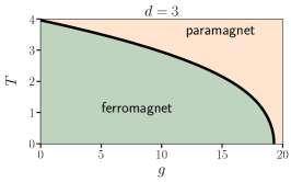
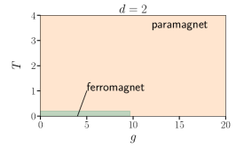
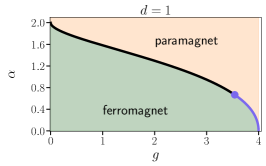
Figure 2: Phase diagrams of the QSM in different dimension: In $d=3$ (left panel) the QSM with nearest neighbor interactions exhibits a thermal critical line and a quantum phase transition at $T=0$. In $d=2$ (center panel) only a quantum phase transition is present. For long-range interactions in $d=1$ (right panel) the zero-temperature critical behavior depends on the long-range exponent $\alpha$. For $\alpha<2/3$ the transition is mean-field (purple).

In addition to the finite temperature transitions of the classical spherical model, the QSM supports a zero-temperature quantum phase transition [11, 13]. If $u_{nm}$ is short-ranged, e.g., nearest neighbor interaction, then the quantum phase transition exists for $d>1$ only. This transition is generally in the same universality class as the thermal transition in the $d+1$ dimensional classical spherical model [11]. Conversely, for long-ranged interactions a quantum phase transition is also present for $d=1$ [11]. The universality class depends on the long range exponent $\alpha$ (see below), although in a simple manner. Generally, $u_{nn}=2\mu$ where $\mu$ is a Lagrange multiplier (chemical potential) that allows to enforce the spherical constraint. This $\mu$ plays the physical role of a mass for the model, or, equivalently, of the inverse correlation length. Hence, the critical line of the model is retrieved from the constraint for $\mu=0$ [11, 13].

Here, we only consider translation invariant systems with periodic boundary conditions such that the Hamiltonian generally decouples in Fourier space. Let us introduce the Fourier transformed operators as

$$x_{n}=\frac{1}{\sqrt{V}}\sum_{k\in\mathcal{B}}e^{\mathrm{i}kn}q_{k},\qquad p_{n}=\frac{1}{\sqrt{V}}\sum_{k\in\mathcal{B}}e^{-\mathrm{i}kn}\pi_{k}$$ (2)

with the $d$ dimensional Brioullin zone $\mathcal{B}$. We recast the QSM Hamiltonian in the form

$$H=\sum_{k\in\mathcal{B}}\frac{g}{2}\pi_{k}\pi_{-k}+\frac{u_{k}}{2}q_{k}q_{-k}=\sum_{k\in\mathcal{B}}E_{k}\left(b_{k}^{\dagger}b_{k}+\frac{1}{2}\right)$$ (3)

with $u_{k}$ being the Fourier transform of the interaction potential $u_{nm}$, $E_{k}=\sqrt{gu_{k}}$ the eigenenergies of the QSM, and $b_{k}$, $b_{k}^{\dagger}$ are adequately chosen bosonic ladder operators. This allows us to explicitly write the equilibrium correlation functions for a system at temperature $T$ as

$$\mathbb{X}_{nm} :=\langle x_{n}x_{m}\rangle=\frac{g}{2V}\sum_{k}e^{\mathrm{i}(n-m)k}\frac{1}{E_{k}}\coth\left(\frac{E_{k}}{2T}\right),$$ (4)

$$\mathbb{P}_{nm} :=\langle p_{n}p_{m}\rangle=\frac{1/g}{2V}\sum_{k}e^{-\mathrm{i}(n-m)k}E_{k}\coth\left(\frac{E_{k}}{2T}\right).$$ (5)

In the following sections we shall focus on entanglement quantities in the QSM. Specifically we consider the following situations

• QSM at finite temperature $T>0$ for $d=3$ with nearest neighbor interactions, viz.,

  $$u(k)=2\mu+2(3-\cos k_{x}-\cos k_{y}-\cos k_{z})$$ (6)

• QSM at $T=0$ for $d=2$ with nearest neighbor interactions, viz.,

  $$u(k)=2\mu+2(2-\cos k_{x}-\cos k_{y})$$ (7)

• QSM at $T=0$ for $d=1$ with long-range interactions [33, 34], viz.,

  $$u(k)=2\mu+\left(2(1-\cos k)\right)^{\alpha/2}.$$ (8)

In Eq. (8), $\alpha$ is the exponent governing the decay with distance of the long-range interactions. The phase diagrams for these systems are depicted in Fig. 2. An important ingredient for the further analysis is to understand the finite-size scaling of the spherical parameter $\mu$. Specifically, we use that $\mu\to 0$ in the ferromagnetic phase and at criticality for $L\to\infty$. For finite $L$ conversely, $\mu$ is always finite. A variety of works have considered this scaling in the classical spherical model, see, e.g., Refs. [35, 36, 37, 38].

3 Entanglement in the quantum spherical model

In this section we introduce several relevant quantum-information-motivated quantities, which have attracted a lot of attention in the statistical and high energy theory communities in the last few years. Consider a many-body quantum system described by a Hilbert space ${\cal{H}}$ and a density matrix $\rho=\ket{\psi_{0}}\bra{\psi_{0}}$ in the corresponding zero-temperature ground state $|\psi_{0}\rangle$. Upon partitioning the system into two parts $A$ and $B$, see Fig. 3, with corresponding Hilbert spaces ${\cal{H}}={\cal{H}}_{A}\otimes{\cal{H}}_{B}$ we can define the reduced density matrix $\rho_{A}$ of subsystem $A$ by tracing out subsystem $B$, viz.,

$$\rho_{A}=\mathrm{Tr}_{B}(\rho).$$ (9)

Although $\rho$ is pure, $\rho_{A}$ is typically a mixed state because the zero-temperature ground-state is not separable. In this scenario, the entanglement entropy

$$S_{A}=-{\mathrm{Tr}}\rho_{A}\log\rho_{A}$$ (10)

is a measure of entanglement between the two subsystems. In terms of the entanglement spectrum [4], i.e., the eigenvalues $\lambda_{i}$ of the reduced density matrix $\rho_{A}$, we can express the entanglement entropy as [1, 2, 4, 39]

$$S_{A}=-\sum_{j}\lambda_{j}\ln\lambda_{j}.$$ (11)

If conversely, the density matrix $\rho$ is not pure, e.g., at finite temperature, or if $\rho$ is pure but one is interested in the entanglement between two non-complementary regions (see Fig. 3 c), then the von Neumann entropy is not a good entanglement witness. A useful quantifier in these cases is the logarithmic negativity [40, 41, 42, 43, 44, 45].

The negativity is defined from the so-called partially transposed reduced density matrix. Given a partition of $A$ as $A=A_{1}\cup A_{2}$ (see Fig. 3 $c)$), the matrix elements of the partial transpose $\rho_{A}^{T_{2}}$ with respect to the degrees of freedom of $A_{2}$ are defined as

$$\langle\varphi_{1}\varphi_{2}|\rho_{A}^{T_{2}}|\varphi_{1}^{\prime}\varphi_{2}^{\prime}\rangle:=\langle\varphi_{1}\varphi_{2}^{\prime}|\rho_{A}|\varphi_{1}^{\prime}\varphi_{2}\rangle.$$ (12)

Here, $\{\varphi_{1}\}$ and $\{\varphi_{2}\}$ are orthonormal bases for $A_{1}$ and $A_{2}$ respectively. In contrast to the eigenvalues of the reduced density matrix $\rho_{A}$, the eigenvalues $\zeta_{i}$ of $\rho_{A}^{T_{2}}$ can be positive or negative. The logarithmic negativity is then defined as

$${\cal{E}}_{A_{1}:A_{2}}=\ln\mathrm{Tr}|\rho_{A}^{T_{2}}|.$$ (13)

The behavior of the logarithmic negativity has been fully characterized in systems that are described by conformal field theory at zero temperature [46] and at finite temperature [47]. Generally, the negativity follows an area law scaling as observed in a variety of systems, see, e.g., Refs. [48, 49, 50, 14, 51, 15].

Finally, we introduce the entanglement spectrum (ES), viz., $\{\xi_{i}=-\ln(\lambda_{i})\ |\ \lambda_{i}\in\mathrm{spec}(\rho_{A})\}$. The lowest entanglement gap (Schmidt gap) is defined by

$$\delta\xi=\xi_{1}-\xi_{0},$$ (14)

where $\xi_{0}$ and $\xi_{1}$ are the lowest and the first excited ES level, respectively.

The ES has received a lot of attention following the observation that it contains universal information about the edge modes in fractional quantum Hall systems [52]. Subsequently, the ES was investigated in a variety of setups, e.g., in conformal field theory [53, 54, 55, 56], in quantum Hall systems [57, 58, 59, 60, 61, 62], in frustrated and magnetically ordered systems [63, 64, 65, 66, 20, 67, 68, 69, 70, 71, 72, 73, 74, 75] or systems with impurities [76].

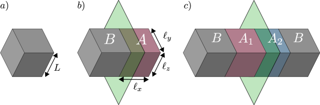
Figure 3: Geometry of partitions: In panel a) a generic three-dimensional system is depicted. In panel b) the system is bipartitioned into two subsystems $A$ and $B$ with $B$ the complement of $A$. In panel c) the subsystems $A_{1}$ and $A_{2}$ are non-complementary.

The main topic of this review is to investigate the entanglement-related quantities introduced above in the QSM in $d=1$, $d=2$ and $d=3$ spatial dimensions.

Since the QSM is mappable to a Gaussian system of bosons (cf. Eq. (3)), entanglement-related quantities can be extracted from the position and momentum correlators (cf. Eqs. (4) and (5)) ${\mathbb{X}}\equiv\langle x_{n}x_{m}\rangle$ and ${\mathbb{P}}\equiv\langle p_{n}p_{m}\rangle$ (see [22] for a review). First, we consider the correlators restricted to subsystem $A$, denoting them as ${\mathbb{X}}[A]$ and ${\mathbb{P}}[A]$. The single-particle eigenvalues $\epsilon_{i}$, with $i\in[1,|A|]$, of the entanglement Hamiltonian $H_{A}$, which is defined as $\rho_{A}=\exp(-H_{A})$, are readily related to the eigenvalues $e_{i}$ of the matrix product $\mathbb{C}_{A}={\mathbb{X}}[A]{\mathbb{P}}[A]$, viz.,

$$\sqrt{e_{i}}=\frac{1}{2}\coth\left(\frac{\epsilon_{i}}{2}\right).$$ (15)

The eigenvalues of the entanglement Hamiltonian $H_{A}$ are constructed by filling the single-particle levels $\epsilon_{i}$ in all possible ways. This allows also to obtain the von Neumann entropy $S_{\mathrm{vN}}$ in terms of the eigenvalues $e_{j}$ as

$$S_{\mathrm{vN}}=\sum_{j}\left[\left(\sqrt{e_{j}}+\frac{1}{2}\right)\ln\left(\sqrt{e_{j}}+\frac{1}{2}\right)-\left(\sqrt{e_{j}}-\frac{1}{2}\right)\ln\left(\sqrt{e_{j}}-\frac{1}{2}\right)\right].$$ (16)

Hence, diagonalizing $\mathbb{C}_{A}$ allows us to deduce the full entanglement spectrum. In particular, assuming that the single-particle entanglement spectrum levels are ordered as $\epsilon_{1}\leq\epsilon_{2}\leq\cdots\leq\epsilon_{|A|}$, the Schmidt gap is simply given by $\delta\xi=\epsilon_{1}$. For Gaussian bosonic systems, the logarithmic negativity can be constructed from the two-point correlation functions [77]. First, we define the transposed matrix ${\mathbb{P}}[A^{T_{2}}]$ as

$${\mathbb{P}}[A^{T_{2}}]\equiv{\mathbb{R}}[A^{T_{2}}]{\mathbb{P}}[A]{\mathbb{R}}[A^{T_{2}}],$$ (17)

where the matrix ${\mathbb{R}}[A^{T_{2}}]$ acts as the identity matrix on $A_{1}$ and as minus the identity matrix on $A_{2}$. The eigenvalues $\nu_{i}^{2}$ of ${\mathbb{X}}[A]{\mathbb{P}}[A^{T_{2}}]$ form the single-particle negativity spectrum. In terms of them the negativity can be written as [77]

$${\cal{E}}=\sum_{i}{\mathrm{max}}(0,-\ln(2\nu_{i})).$$ (18)

4 Quantum and classical fluctuations at finite temperature criticality

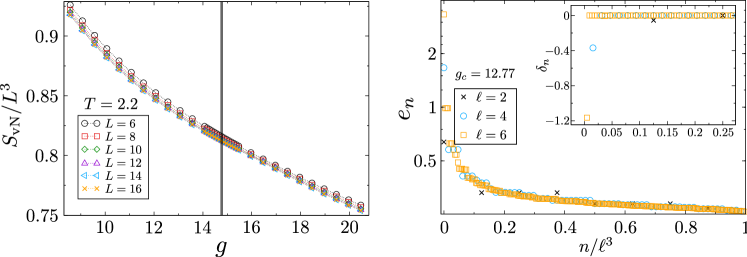
Figure 4: von Neumann entropy and entanglement spectrum: (Left panel) Volume-law scaling of the von Neumann entropy across the finite-temperature transition in the three-dimensional QSM. Singular terms are present but they vanish at the transition and are overshadowed by the analytic background. Non-analytic contributions are more visible in the entanglement spectrum (notice the divergence of the largest negative single-particle ES level in the right panel). In the inset we show $\delta_{n}$ (cf. Eq. (19)), which measures the nonanalyticity of the levels across the transition. Here $\delta_{n}\neq 0$ signals nonanalytic behavior.

Understanding the interplay of classical and quantum fluctuations is an important but challenging task [78, 79, 75]. One way of approaching this question is by studying entanglement witnesses in the vicinity of a finite temperature phase transition that is driven by classical fluctuations. It has been observed that a variety of entanglement witnesses are sensitive to classical criticality. For instance, it has been shown that the negativity develops cusp-like singularities [14, 51]. In this section we review our investigation from Ref. [15] of entanglement-related quantities at the finite-temperature transition in the $d=3$ dimensional QSM, see Fig. 2 (left panel).

First, we discuss the von Neumann entropy $S_{\rm vN}$ for the bipartition of the system into two equal parts (see Fig. 3). As we mentioned in Sec. 3, $S_{\rm vN}$ is not a valid entanglement witness at finite temperature. In fact, the von Neumann entropy becomes the standard thermal entropy at finite temperature. Indeed, as shown in Fig. 4 (left panel), $S_{\mathrm{vN}}$ satisfies a standard volume-law scaling. Being sensitive to both quantum and classical correlations, the von Neumann entropy overestimates the amount of entanglement, which is expected to scale with the boundary between the two subsystems. Moreover, the von Neumann entropy does not show any singularity at the transition. This happens because singular terms, although they are present, vanish at the critical point, and are overshadowed by the analytic background. Singularities are more visible in the single-particle entanglement spectrum, as illustrated in the right panel of Fig. 4. In the figure we show the entanglement spectrum for two adjacent blocks of linear size $\ell$ embedded in an infinite system. The eigenvalues quickly decay upon increasing their index and most of them satisfy $e_{n}\approx 1/4$. Clearly, only those eigenvalues with low index can yield potentially singular contributions. In the inset we investigate the singularity using the quantity

$$\delta_{n}=(e_{n})_{+}^{\prime}-(e_{n})_{-}^{\prime}$$ (19)

that measures the difference of the right and left derivatives of $e_{n}$ with respect to $g$ at $g_{c}$. Clearly $\delta_{n}\neq 0$ indicates a non-analyticity and we observe this for small $n$.

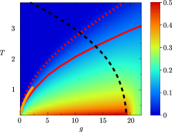
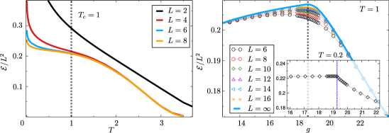
Figure 5: Entanglement negativity in the three-dimensional QSM: The left panel is an overview of the negativity in the $g-T$ plane, with $T$ the temperature and $g$ the quantum coupling (cf. Eq. (1)). Here we always consider the half-system negativity. The critical line is reported as black dashed line. The red-dashed line is the death line above which the negativity is exactly zero. The death line as extracted from the negativity between two adjacent spins is reported as red solid line. The orange solid line is the behavior as $\sqrt{g}$ at small $g$. The centre (right) panel shows the negativity across the phase transition varying the temperature (quantum parameter). In the right panel the continuous line is the result in the thermodynamic limit. The inset shows the behavior of the negativity at $T=0.2$, i.e., close to the quantum phase transition.

Next, we discuss the entanglement negativity. As outlined in Sec. 3, the negativity is a proper entanglement witness, and as such obeys an area law, see center and right panel in Fig. 5. Crossing the thermal transition at fixed finite $T$, i.e., changing the quantum driving parameter $g$ the negativity decays slowly as $1/g$ for large $g$, see Fig. 5 right panel. This is in contrast to the behavior when crossing the transition with the temperature $T$ at fixed $g$, as depicted in the center panel of Fig. 5. Here, the negativity shows a sudden death after and remains exactly zero for increasing $T$. We also see that the negativity does not show any cusp singularity across the finite temperature transition but develops a cusp when approaching low temperatures (see inset right panel in Fig. 5). This signals that singularities, although present, are strongly suppressed. Furthermore, in Fig. 5 (left panel), we map out the negativity in the full phase diagram. In the figure the dashed line is the critical line separating the paramagnetic and the ferromagnetic phase. We observe that the negativity generally attains a maximum at the quantum phase transition, hinting at a strongly entangled quantum state. We also observe that the negativity increases upon lowering the temperature and is largest for $T=0$. We also highlight the numerical death line in Fig. 5 (dotted line in the left panel) above which the negativity is zero.

Interestingly, most of these findings can be quantitatively understood considering two adjacent sites embedded in an infinite system. This setup allows for analytic investigations as shown in Ref. [15]. For large $g$ and constant $T$, this approach qualitatively predicts the slow negativity decay from Fig. 5 (right panel), viz.,

$$\mathcal{E}=-\ln\left(\frac{g-2}{g}\right)\stackrel{{\scriptstyle g\to\infty}}{{\simeq}}\frac{2}{g}.$$ (20)

Similarly, it predicts the existence of the death line (continuous line in the figure), and correctly captures its onset for small $g$ as $\sqrt{g}$, see Fig. 5 (left panel).

5 Entanglement gap at 2D quantum criticality

As we have seen in Sec. 4 the low-laying entanglement spectrum encodes relevant information about the critical properties of the system. To further investigate this aspect we review in this section our studies in Refs. [16, 17] of the behavior of the Schmidt gap at quantum criticality and in the ferromagnetic phase in the two dimensional QSM. Interest in the behavior of the Schmidt gap has spiked in the last decade.

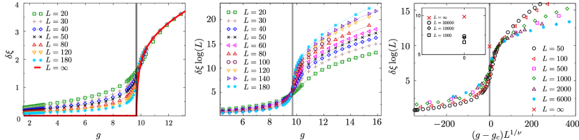
Figure 6: Overview of the entanglement gap in the two-dimensional QSM: The left panel shows the gap $\delta\xi$ across the whole phase diagram. We observe distinct behaviors in the paramagnetic phase (finite gap) and the ferromagnetic phase (vanishing gap). We always consider the half-system entanglement spectrum. The continuous line in the left panel is the result in the thermodynamic limit [16]. In the center panel we show the rescaled gap $\delta\xi\ln(L)$. At the critical point the gap decays as $1/\ln(L)$, which implies that the rescaled gap should exhibit a crossing. In the right panel we plot $\delta\xi\ln(L)$ versus $(g-g_{c})L^{1/\nu}$. Upon approaching the thermodynamic limit $L\to\infty$ a data collapse is expected. The cross symbol is $\delta\xi\ln(L)$ at $g=g_{c}$ and $L\to\infty$. Still, subleading terms are too large to observe the collapse, as confirmed in the inset.

In the left panel of Fig. 6 we show the numerical findings for the behavior of $\delta\xi$ across the phase diagram, see Fig. 2. Here, we consider a bipartition of the system into two equal halves. In the paramagnetic regime, we observe that the gap converges rapidly to a finite number upon increasing the linear system size $L$. Hence, the gap remains finite in the thermodynamic limit $L\to\infty$. Conversely, the behavior at the critical point [16] and in the ferromagnetic phase [17] differs from that in the paramagnetic phase. In the ferromagnetic phase, the entanglement gap scales as [17]

$$\delta\xi\simeq\frac{\Omega}{\sqrt{L\ln(L)}},$$ (21)

where the constant $\Omega$ is known analytically [17], and depends on low-energy properties of the QSM and on the geometry. For instance, $\Omega$ is sensitive to the presence of corners in the boundary between $A$ and the rest. Hence, the gap closes algebraically, involving logarithmic corrections. At criticality we find that the Schmidt gap still closes, i.e., $\delta\xi\to 0$ albeit significantly slower. Precisely, the gap vanishes as [15]

$$\delta\xi\simeq\frac{\pi^{2}}{\ln(L)}.$$ (22)

This result is obtained for the bipartition into equal halves as follows. Since we use periodic boundary conditions in both directions, and the bipartition does not introduce corners, the momentum $k_{y}$ remains a good quantum number also for the reduced density matrix. This allows to exploit dimensional reduction [80] mapping the problem to a one-dimensional one. Hence, we may use the analytical result for a one dimensional massive harmonic chain [22] in order to obtain Eq. (22). Since the harmonic chain result is derived using the corner transfer matrix on two infinite halves, whereas we have periodic boundary conditions also along the $x$ direction, Eq. (22) is exact only at leading order in $L$. Our results are numerically confirmed in Fig. 7. In the figure we consider the largest eigenvalue $e_{1}$ of $\mathbb{C}_{A}$ (see Section 3). This is related to the entanglement gap via Eq. (15) and Eq. (14). In particular, a diverging $e_{1}$ implies a vanishing entanglement gap. Fig. 7 shows that the leading behavior of $e_{1}$ at large $L$ is correctly captured by the analytic result (full line). Again, Fig. 7 confirms that the entanglement gap is finite in the paramagnetic phase, whereas in the ordered phase a faster divergence is observed (cf. Eq. (21)).

In the right panel of Fig. 7 we subtract the analytic prediction for the leading behavior of $e_{1}$. The continuous line is a fit to $A_{0}+A_{1}\ln(L)$. The result of the fit confirms the presence of a logarithmic correction to the leading behavior.

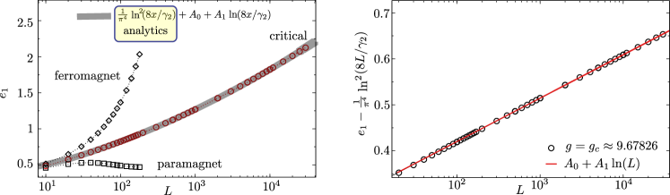
Figure 7: Scaling of the largest eigenvalue $e_{1}$ of $\mathbb{C}_{A}$: The left panel shows the scaling of $e_{1}$ in the paramagnetic and the ferromagnetic phase as well as at criticality in the $2d$ QSM. In the paramagnetic phase $e_{1}$ converges to a finite value and in the ferromagnetic phase $e_{1}$ diverges (hence $\delta\xi\to 0$). At criticality we see a slower divergence than in the ordered phase. The full grey line is a fit to $1/\pi^{4}\ln(8L/\gamma_{2})+A_{0}+A_{1}\ln(8L/\gamma_{2})$, with $A_{0},A_{1}$ fitting parameters. The leading part $\sim\ln^{2}(L)$ is obtained analytically. Here $\gamma_{2}$ is a known constant [16]. In the right panel we investigate the subleading logarithmic term.

6 Entanglement gap and symmetry breaking in the QSM

In the ferromagnetically ordered phase of the QSM, the dispersion develops a zero mode, which reflects the Goldstone mode associated to symmetry breaking. This implies that the position correlation function (see Eq. (4)) diverges. Here we show that this fact is sufficient to fully determine the scaling of the entanglement gap. First, the divergence in Eq. (4) is reflected in the fact that the eigenvector of $\mathbb{C}_{A}$ associated with the largest eigenvalue becomes flat in the thermodynamic limit [16, 17]. Hence, we may rewrite the position correlator up to leading order as

$$\mathbb{X}\simeq\chi^{x}\ket{1}\bra{1},\quad\mathrm{with}\,\,\chi^{x}\propto L,$$ (23)

with $\ket{1}$ being a normalized flat vector. First, we note that $\bra{1}\mathbb{X}\ket{1}=\chi^{x}$. Furthermore, it is easy to verify that $\bra{1}\mathbb{P}$ and $\ket{1}$ are left and right eigenvectors of $\mathbb{C}$. Both correspond to the largest (diverging) eigenvalue $e_{1}$. Hence, it is straightforward to identify

$$e_{1}=\bra{1}\mathbb{X}\ket{1}\bra{1}\mathbb{P}\ket{1}:=\chi^{x}\chi^{t},$$ (24)

where $\chi^{t}:=\langle 1|\mathbb{P}|1\rangle$. Here we should observe that $\chi^{x}$ resembles a susceptibility for the position variables $x_{i}$, whereas $\chi^{t}$ is the susceptibility of the $p_{i}$. Eq. (24) establishes a remarkable correspondence between the entanglement gap and standard quantities such as $\chi^{x}$ and $\chi^{t}$. A similar decomposition as in Eq. (24) was employed in Ref. [81] to treat the zero-mode contribution to entanglement in the harmonic chain.

We now verify numerically that, as expected, the eigenvector of $\mathbb{C}_{A}$ corresponding to its largest eigenvalue $e_{1}$ becomes flat in the ferromagnetic phase, which ensures the validity of Eq. (24). Our results are reported in Fig. 8 where we show the overlap $\varphi$ between the flat vector and the exact eigenvector of the correlation matrix. At criticality, the eigenvector is not flat in the thermodynamic limit $L\to\infty$ (see Fig. 8). On the other hand, below the critical point the eigenvector becomes flat in the thermodynamic limit.

6.1 Entanglement gap in the ferromagnetic phase of the 2D QSM

Let us now discuss the application of Eq. (24) in the ordered phase of the two-dimensional QSM. To employ Eq. (24) we have to evaluate the flat vector expectation values of the position and momentum correlation matrix. The standard way is to decompose them in a thermodynamic and a finite size part, i.e.,

$$\bra{1}\mathbb{X}\ket{1}=\bra{1}\mathbb{X}^{\rm(th)}\ket{1}+\bra{1}\mathbb{X}^{(L)}\ket{1}$$ (25)

and similar for $\bra{1}\mathbb{P}\ket{1}$, using the Poisson summation formula

$$\sum_{n=a}^{b}f(n)=\frac{f(a)+f(b)}{2}+\int_{a}^{b}f(x){\mathrm{d}}x+2\sum_{p=1}^{\infty}\int_{a}^{b}f(x)\cos(2\pi px){\mathrm{d}}x.$$ (26)

The FSS of these contributions is then obtained from the FSS of the spherical parameter $\mu$ and from standard methods such as stationary phase methods, Euler-Maclaurin formulas, and Mellin transform techniques. One finds [17]

$$\bra{1}\mathbb{X}^{\rm(th)}\ket{1}\sim L^{2},\quad\bra{1}\mathbb{X}^{(L)}\ket{1}\sim L^{2},\quad\bra{1}\mathbb{P}^{\rm(th)}\ket{1}\sim\frac{\ln(L)}{L},\quad\bra{1}\mathbb{P}^{(L)}\ket{1}\sim\frac{\ln(L)}{L}.$$ (27)

Notice that $\chi^{t}$ vanishes at $L\to\infty$. Thus, the entanglement gap scales as $\delta\xi\sim 1/\sqrt{L\ln(L)}$. This is in agreement with our numerical simulations [17]. Furthermore, it has been suggested that for continuous symmetries, the gap should vanish as [20] $\delta\xi\sim 1/(L\ln(L))$ which differs from our result. This could be specific of the QSM, although the issue would require further clarification.

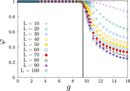
Figure 8: Lowest eigenvector of $\mathbb{C}_{A}$: We show the overlap $\varphi$ between the eigenvector of $\mathbb{C}_{A}$ corresponding to the largest eigenvalue and the flat vector. In the ordered phase of the QSM one has that $\varphi\to 1$ in the thermodynamic limit. This is not the case at the critical point and in the ferromagnetic phase.

Finally, one can assume that the decomposition in Eq. (24) also holds at the critical point [16]. This gives

$$\bra{1}\mathbb{X}^{\rm(th)}\ket{1}\sim L,\quad\bra{1}\mathbb{X}^{(L)}\ket{1}\sim L,\quad\bra{1}\mathbb{P}^{\rm(th)}\ket{1}\sim\frac{\ln(L)}{L},\quad\bra{1}\mathbb{P}^{(L)}\ket{1}\sim\frac{\ln(L)}{L}.$$ (28)

This implies that the entanglement gap vanishes as $\delta\xi\sim 1/\sqrt{\ln(L)}$. Although this scaling is not correct, reflecting that Eq. (24) does not hold at criticality, it still captures the logarithmic character of the entanglement gap.

7 Entanglement gap in 1D QSM with long-range interactions

Recently, there has been increasing interest in quantum systems with long-range interactions [82, 83], also due to significant experimental advances [84]. Since long-range interactions affect the structure of quantum correlations between subsystems, it is interesting to study entanglement witnesses in these systems. Indeed, the study of entanglement in long-range systems has seen a significant surge of interest [85, 86, 87, 88, 89, 90, 91, 92, 93, 94, 95].

Arguably one of the paradigmatic systems is the long-range QSM at $T=0$ in one spatial dimension that we introduced in section 2. In terms of the long-range exponent $\alpha$ the interaction strength between two lattice sites behaves as $u_{nm}\sim|n-m|^{-(1+\alpha)}$. The parameter $\alpha$ satisfies $0\leq\alpha<2$ where $\alpha=2$ would correspond to nearest-neighbor interaction and $\alpha=0$ is essentially an infinite range interaction. The zero temperature phase diagram is reported in Fig. 2 (right panel). For $0<\alpha<2/3$ the transition is of the mean-field type, whereas for $2/3<\alpha<2$ the model shows a non-mean-field transition [11, 18].

Crucially, despite the long-range nature of the model, in the ordered phase Eq. (24) holds true. Thus, the study of the scaling of the entanglement gap proceeds as outlined in section 6. The susceptibilities $\chi^{x}$ and $\chi^{t}$ can be analyzed for $L\to\infty$ with regularization techniques involving the Mellin transform [96, 18] (details can be found in Ref. [18]).

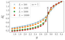
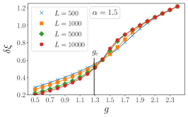
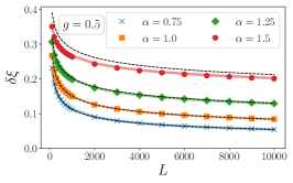
Figure 9: Entanglement gap in the long-range $1d$ QSM: The left and center panel show the entanglement gap for different values of the long-range exponent $\alpha$ ($\alpha=1$ and $\alpha=1.5$ respectively) across the phase transition. We observe a qualitative difference between the paramagnetic phase and the ferromagnetic phase. The right panel shows the closure of the entanglement gap for different values of $\alpha$ in the ferromagnetic phase. Symbols are numerical results from exact diagonalization and the continuous line corresponds to Eq. (24). Black dashed lines correspond to the analytical prediction.

In Fig. 9 we present in the left and center panel a numerical analysis of the entanglement gap across the phase diagram. We observe that $\delta\xi$ remains finite in the paramagnetic phase, whereas it shows a vanishing behavior in the ferromagnetic phase upon increasing $L$. As in the two dimensional QSM it is useful to decompose the correlation matrices into a thermodynamic and a finite size part. Using Mellin techniques we obtain [18]

$$\bra{1}\mathbb{X}^{\rm(th)}\ket{1}\sim L,\quad\bra{1}\mathbb{X}^{(L)}\ket{1}\sim L^{\alpha/2},\quad\bra{1}\mathbb{P}^{\rm(th)}\ket{1}\sim L^{-\alpha/2},\quad\bra{1}\mathbb{P}^{(L)}\ket{1}\sim L^{-\alpha/2}.$$ (29)

Further details such as the precise prefactors, subleading contributions, the behavior at criticality and the numerical benchmarks for all these results can be found in Ref. [18]. These results allow us to deduce the entanglement gap using Eq. (24). We obtain

$$\delta\xi\sim L^{-(1/2-\alpha/4)}.$$ (30)

In the right panel of Fig. 9 we show a comparison of exact diagonalization results and Eq. (30), finding perfect agreement. Note that the entanglement gap decays algebraically with $L$, and multiplicative logarithmic corrections are absent. This differs strictly from the logarithmic behavior encountered in the previous section.

8 Summary and Conclusions

We provided an overview of several results on the entanglement scaling in the QSM. In particular, we investigated a variety of scenarios comprising $d=1,2,3$ dimensional quantum systems with long and short range interactions.

Precisely, we discussed the interplay of classical and quantum fluctuations at thermal transitions in the $3d$ QSM. We presented results for the entanglement entropy, the entanglement negativity and the entanglement spectrum in Sec. 4. In particular, we mapped out the negativity across the whole phase diagram (see Fig. 5). A more detailed analysis can be found in our work in Ref. [15]. In Sec. 5 and Sec. 6 we focussed on the quantum phase transition and on the ferromagnetic phase at zero temperature in two spatial dimensions. We discussed the behavior of the entanglement gap in the different quantum phases and at criticality. We showed that the entanglement gap is capable of detecting criticality in the QSM, although logarithmic corrections are present. We refer to Refs. [16, 17] for more details on the entanglement spectrum, the precise finite-size scaling, and for the study of the effect of corners in the entanglement spectrum. Finally, we reviewed entanglement properties of a one dimensional spherical quantum chain with long-range interactions [18]. Again, we considered the behavior of the entanglement gap across the zero temperature quantum phase transition for different long-range interactions. Remarkably, the QSM allows for a detailed analytical investigation of the entanglement gap in the ordered phase of the model. In particular, it is possible to understand how the entanglement gap is affected by the long-range nature of the interactions.

The spherical model - here in its quantum formulation - has again proven itself as a remarkably useful tool to study collective phenomena in strongly interacting many-body systems. Clearly, the QSM will continue to serve as a reference system for future studies of entanglement-related quantities. For example it would be interesting to further investigate the influence of corners on the entanglement patterns. Furthermore, it would be enlightening to consider the QSM on quasi two-dimensional structures, such as ladders. It would also be interesting to study the influence of disorder, or explore the full entanglement Hamiltonian explicitly. Moreover, it has been shown that the criticality in the QSM (in and out of equilibrium) can be exploited as a resource in quantum metrology [97]. It would be interesting to explore to which extend entanglement might affect and support quantum metrology protocols. Furthermore, non-equilibrium and relaxational quantum dynamics has been extensively studied in the QSM in the past years [98, 99, 100, 101, 102, 103]. It would be interesting to derive the spreading of entanglement in such scenarios in the QSM, possibly exploiting the results from Refs. [104, 105, 106, 103]. An intriguing idea is to study the entanglement using the Kibble-Zurek dynamics [107, 108].

References

References

- [1] Amico L, Fazio R, Osterloh A and Vedral V 2008 Rev. Mod. Phys. 80(2) 517–576 URL https://link.aps.org/doi/10.1103/RevModPhys.80.517
- [2] Eisert J, Cramer M and Plenio M B 2010 Rev. Mod. Phys. 82(1) 277–306 URL https://link.aps.org/doi/10.1103/RevModPhys.82.277
- [3] Calabrese P, Cardy J and Doyon B 2009 Journal of Physics A: Mathematical and Theoretical 42 500301 URL https://doi.org/10.1088/1751-8121/42/50/500301
- [4] Laflorencie N 2016 Physics Reports 646 1–59 URL https://doi.org/10.1016/j.physrep.2016.06.008
- [5] Horodecki R, Horodecki P, Horodecki M and Horodecki K 2009 Rev. Mod. Phys. 81(2) 865–942 URL https://link.aps.org/doi/10.1103/RevModPhys.81.865
- [6] Baxter R 2016 Exactly Solved Models in Statistical Mechanics (Elsevier Science) ISBN 9781483265940 URL https://books.google.co.uk/books?id=egtcDAAAQBAJ
- [7] Berlin T H and Kac M 1952 Physical Review 86 821–835 ISSN 0031-899X URL https://link.aps.org/doi/10.1103/PhysRev.86.821
- [8] Lewis H W and Wannier G H 1952 Physical Review 88 682–683 ISSN 0031-899X URL http://link.aps.org/doi/10.1103/PhysRev.86.821http://link.aps.org/doi/10.1103/PhysRev.88.682.2
- [9] Obermair G 1972 A dynamical spherical model Dynamical Aspects of critical phenomena (New York: Gordon and Breach) p 10
- [10] Henkel M and Hoeger C 1984 Zeitschrift für Physik B Condensed Matter 55 67–73 ISSN 0722-3277 URL http://link.springer.com/10.1007/BF01307503
- [11] Vojta T 1996 Physical Review B 53 710 ISSN 0163-1829 URL http://link.aps.org/abstract/PRB/v53/p710{%}5Cnpapers2://publication/uuid/A5F04936-25CE-4C76-906D-78E3C75CD931
- [12] Bienzobaz P and Salinas S 2012 Physica A: Statistical Mechanics and its Applications 391 6399 – 6408 ISSN 0378-4371 URL http://www.sciencedirect.com/science/article/pii/S0378437112006929
- [13] Wald S and Henkel M 2015 Journal of Statistical Mechanics: Theory and Experiment 07006 34 ISSN 17425468 (Preprint 1503.06713) URL http://arxiv.org/abs/1503.06713
- [14] Lu T C and Grover T 2019 Physical Review B 99 075157 ISSN 2469-9950 (Preprint 1808.04381) URL https://link.aps.org/doi/10.1103/PhysRevB.99.075157
- [15] Wald S, Arias R and Alba V 2020 Journal of Statistical Mechanics: Theory and Experiment 2020 033105 URL https://doi.org/10.1088%2F1742-5468%2Fab6b19
- [16] Wald S, Arias R and Alba V 2020 Phys. Rev. Research 2(4) 043404 URL https://link.aps.org/doi/10.1103/PhysRevResearch.2.043404
- [17] Alba V 2021 SciPost Phys. 10 056 URL https://scipost.org/10.21468/SciPostPhys.10.3.056
- [18] Wald S, Arias R and Alba V 2023 Entanglement gap in 1d long-range quantum spherical models URL https://arxiv.org/abs/2301.09143
- [19] Metlitski M A, Fuertes C A and Sachdev S 2009 Phys. Rev. B 80(11) 115122 URL https://link.aps.org/doi/10.1103/PhysRevB.80.115122
- [20] Metlitski M A and Grover T 2011 Entanglement entropy of systems with spontaneously broken continuous symmetry (Preprint arXiv:1112.5166)
- [21] Whitsitt S, Witczak-Krempa W and Sachdev S 2017 Phys. Rev. B 95(4) 045148 URL https://link.aps.org/doi/10.1103/PhysRevB.95.045148
- [22] Peschel I and Eisler V 2009 Journal of Physics A: Mathematical and Theoretical 42 504003 URL https://doi.org/10.1088/1751-8113/42/50/504003
- [23] Ising T, Folk R, Kenna R, Berche B and Holovatch Y 2017 Journal of Physical Studies 21 URL https://doi.org/10.30970/jps.21.3002
- [24] Taroni A 2015 Nature Physics 11 997–997 ISSN 1745-2481 URL https://doi.org/10.1038/nphys3595
- [25] Okamoto Y 2021 Scientific Reports 11 23703 ISSN 2045-2322 URL https://doi.org/10.1038/s41598-021-03050-z
- [26] BRUSH S G 1967 Rev. Mod. Phys. 39(4) 883–893 URL https://link.aps.org/doi/10.1103/RevModPhys.39.883
- [27] Bartashevich P and Mostaghim S 2019 Ising model as a switch voting mechanism in collective perception Progress in Artificial Intelligence ed Moura Oliveira P, Novais P and Reis L P (Cham: Springer International Publishing) pp 617–629 ISBN 978-3-030-30244-3
- [28] D’Angelo F and Böttcher L 2020 Phys. Rev. Res. 2(2) 023266 URL https://link.aps.org/doi/10.1103/PhysRevResearch.2.023266
- [29] Yeomans J 1992 Statistical Mechanics of Phase Transitions (Clarendon Press) ISBN 9780191589706 URL https://books.google.co.uk/books?id=3IUVSvOUtTMC
- [30] Pelissetto A and Vicari E 2002 Physics Reports 368 549–727 ISSN 0370-1573 URL https://www.sciencedirect.com/science/article/pii/S0370157302002193
- [31] Nishimori H and Ortiz G 2010 Elements of Phase Transitions and Critical Phenomena (Oxford University Press) ISBN 9780199577224 URL https://doi.org/10.1093/acprof:oso/9780199577224.001.0001
- [32] Stanley H E 1968 Phys. Rev. 176(2) 718–722 URL https://link.aps.org/doi/10.1103/PhysRev.176.718
- [33] Zoia A, Rosso A and Kardar M 2007 Phys. Rev. E 76(2) 021116 URL https://link.aps.org/doi/10.1103/PhysRevE.76.021116
- [34] Nezhadhaghighi M G and Rajabpour M A 2012 EPL (Europhysics Letters) 100 60011 URL https://doi.org/10.1209/0295-5075/100/60011
- [35] Barber M N and Fisher M E 1973 Annals of Physics 77 1–78 ISSN 0003-4916 URL https://www.sciencedirect.com/science/article/pii/0003491673904090
- [36] Brankov J G and Tonchev N S 1988 Journal of Statistical Physics 52 143–159 ISSN 1572-9613 URL https://doi.org/10.1007/BF01016408
- [37] Brézin E 1982 Journal de Physique 43 15–22
- [38] Singh S and Pathria R 1985 Physical Review B 31 4483
- [39] Calabrese P, Cardy J and Doyon B 2009 Journal of Physics A: Mathematical and Theoretical 42 500301 URL https://dx.doi.org/10.1088/1751-8121/42/50/500301
- [40] Lee J, Kim M S, Park Y J and Lee S 2000 Journal of Modern Optics 47 2151–2164 (Preprint https://doi.org/10.1080/09500340008235138) URL https://doi.org/10.1080/09500340008235138
- [41] Eisert J and Plenio M B 1999 Journal of Modern Optics 46 145–154 (Preprint https://www.tandfonline.com/doi/pdf/10.1080/09500349908231260) URL https://www.tandfonline.com/doi/abs/10.1080/09500349908231260
- [42] Vidal G and Werner R F 2002 Phys. Rev. A 65(3) 032314 URL https://link.aps.org/doi/10.1103/PhysRevA.65.032314
- [43] Plenio M B 2005 Phys. Rev. Lett. 95(9) 090503 URL https://link.aps.org/doi/10.1103/PhysRevLett.95.090503
- [44] Peres A 1996 Phys. Rev. Lett. 77(8) 1413–1415 URL https://link.aps.org/doi/10.1103/PhysRevLett.77.1413
- [45] Życzkowski K, Horodecki P, Sanpera A and Lewenstein M 1998 Phys. Rev. A 58(2) 883–892 URL https://link.aps.org/doi/10.1103/PhysRevA.58.883
- [46] Calabrese P, Cardy J and Tonni E 2012 Phys. Rev. Lett. 109(13) 130502 URL https://link.aps.org/doi/10.1103/PhysRevLett.109.130502
- [47] Calabrese P, Cardy J and Tonni E 2014 Journal of Physics A: Mathematical and Theoretical 48 015006 URL https://dx.doi.org/10.1088/1751-8113/48/1/015006
- [48] Nobili C D, Coser A and Tonni E 2016 Journal of Statistical Mechanics: Theory and Experiment 2016 083102 URL https://dx.doi.org/10.1088/1742-5468/2016/08/083102
- [49] Eisler V and Zimborás Z 2016 Phys. Rev. B 93(11) 115148 URL https://link.aps.org/doi/10.1103/PhysRevB.93.115148
- [50] Shapourian H and Ryu S 2019 Journal of Statistical Mechanics: Theory and Experiment 2019 043106 URL https://dx.doi.org/10.1088/1742-5468/ab11e0
- [51] Lu T C and Grover T 2020 Phys. Rev. Res. 2(4) 043345 URL https://link.aps.org/doi/10.1103/PhysRevResearch.2.043345
- [52] Li H and Haldane F D M 2008 Phys. Rev. Lett. 101(1) 010504 URL https://link.aps.org/doi/10.1103/PhysRevLett.101.010504
- [53] Calabrese P and Lefevre A 2008 Phys. Rev. A 78(3) 032329 URL https://link.aps.org/doi/10.1103/PhysRevA.78.032329
- [54] Läuchli A M 2013 Operator content of real-space entanglement spectra at conformal critical points (Preprint arXiv:1303.0741)
- [55] Alba V, Calabrese P and Tonni E 2017 Journal of Physics A: Mathematical and Theoretical 51 024001 URL https://doi.org/10.1088%2F1751-8121%2Faa9365
- [56] Cardy J 2015 The entanglement gap in cfts, talk at the kitp conference ”closing the entanglement gap: Quantum information, quantum matter, and quantum fields”. URL http://online.kitp.ucsb.edu/online/entangled-c15/cardy/
- [57] Thomale R, Arovas D P and Bernevig B A 2010 Phys. Rev. Lett. 105(11) 116805 URL https://link.aps.org/doi/10.1103/PhysRevLett.105.116805
- [58] Läuchli A M, Bergholtz E J, Suorsa J and Haque M 2010 Phys. Rev. Lett. 104(15) 156404 URL https://link.aps.org/doi/10.1103/PhysRevLett.104.156404
- [59] Haque M, Zozulya O and Schoutens K 2007 Phys. Rev. Lett. 98(6) 060401 URL https://link.aps.org/doi/10.1103/PhysRevLett.98.060401
- [60] Thomale R, Sterdyniak A, Regnault N and Bernevig B A 2010 Phys. Rev. Lett. 104(18) 180502 URL https://link.aps.org/doi/10.1103/PhysRevLett.104.180502
- [61] Hermanns M, Chandran A, Regnault N and Bernevig B A 2011 Phys. Rev. B 84(12) 121309(R) URL https://link.aps.org/doi/10.1103/PhysRevB.84.121309
- [62] Chandran A, Hermanns M, Regnault N and Bernevig B A 2011 Phys. Rev. B 84(20) 205136 URL https://link.aps.org/doi/10.1103/PhysRevB.84.205136
- [63] Poilblanc D 2010 Phys. Rev. Lett. 105(7) 077202 URL https://link.aps.org/doi/10.1103/PhysRevLett.105.077202
- [64] Cirac J I, Poilblanc D, Schuch N and Verstraete F 2011 Phys. Rev. B 83(24) 245134 URL https://link.aps.org/doi/10.1103/PhysRevB.83.245134
- [65] De Chiara G, Lepori L, Lewenstein M and Sanpera A 2012 Phys. Rev. Lett. 109(23) 237208 URL https://link.aps.org/doi/10.1103/PhysRevLett.109.237208
- [66] Alba V, Haque M and Läuchli A M 2012 Phys. Rev. Lett. 108(22) 227201 URL https://link.aps.org/doi/10.1103/PhysRevLett.108.227201
- [67] Alba V, Haque M and Läuchli A M 2012 Journal of Statistical Mechanics: Theory and Experiment 2012 P08011 URL https://doi.org/10.1088/1742-5468/2012/08/p08011
- [68] Alba V, Haque M and Läuchli A M 2013 Phys. Rev. Lett. 110(26) 260403 URL https://link.aps.org/doi/10.1103/PhysRevLett.110.260403
- [69] Lepori L, De Chiara G and Sanpera A 2013 Phys. Rev. B 87(23) 235107 URL https://link.aps.org/doi/10.1103/PhysRevB.87.235107
- [70] James A J A and Konik R M 2013 Phys. Rev. B 87(24) 241103 URL https://link.aps.org/doi/10.1103/PhysRevB.87.241103
- [71] Kolley F, Depenbrock S, McCulloch I P, Schollwöck U and Alba V 2013 Phys. Rev. B 88(14) 144426 URL https://link.aps.org/doi/10.1103/PhysRevB.88.144426
- [72] Chandran A, Khemani V and Sondhi S L 2014 Phys. Rev. Lett. 113(6) 060501 URL https://link.aps.org/doi/10.1103/PhysRevLett.113.060501
- [73] Rademaker L 2015 Phys. Rev. B 92(14) 144419 URL https://link.aps.org/doi/10.1103/PhysRevB.92.144419
- [74] Kolley F, Depenbrock S, McCulloch I P, Schollwöck U and Alba V 2015 Phys. Rev. B 91(10) 104418 URL https://link.aps.org/doi/10.1103/PhysRevB.91.104418
- [75] Frérot I and Roscilde T 2016 Phys. Rev. Lett. 116(19) 190401 URL https://link.aps.org/doi/10.1103/PhysRevLett.116.190401
- [76] Bayat A, Johannesson H, Bose S and Sodano P 2014 Nature Communications 5 URL https://doi.org/10.1038/ncomms4784
- [77] Audenaert K, Eisert J, Plenio M B and Werner R F 2002 Phys. Rev. A 66(4) 042327 URL https://link.aps.org/doi/10.1103/PhysRevA.66.042327
- [78] Hauke P, Heyl M, Tagliacozzo L and Zoller P 2016 Nature Physics 12 778–782 ISSN 1745-2481 URL https://doi.org/10.1038/nphys3700
- [79] Gabbrielli M, Smerzi A and Pezzè L 2018 Scientific Reports 8 15663 ISSN 2045-2322 URL https://doi.org/10.1038/s41598-018-31761-3
- [80] Murciano S, Ruggiero P and Calabrese P 2020 Journal of Statistical Mechanics: Theory and Experiment 2020 083102 URL https://doi.org/10.1088/1742-5468/aba1e5
- [81] Botero A and Reznik B 2004 Phys. Rev. A 70(5) 052329 URL https://link.aps.org/doi/10.1103/PhysRevA.70.052329
- [82] Defenu N, Donner T, Macrì T, Pagano G, Ruffo S and Trombettoni A 2021 Long-range interacting quantum systems URL https://arxiv.org/abs/2109.01063
- [83] Defenu N 2021 Proceedings of the National Academy of Sciences 118 e2101785118 (Preprint https://www.pnas.org/doi/pdf/10.1073/pnas.2101785118) URL https://www.pnas.org/doi/abs/10.1073/pnas.2101785118
- [84] Zhang J, Pagano G, Hess P W, Kyprianidis A, Becker P, Kaplan H, Gorshkov A V, Gong Z X and Monroe C 2017 Nature 551 601–604 ISSN 1476-4687 URL https://doi.org/10.1038/nature24654
- [85] Koffel T, Lewenstein M and Tagliacozzo L 2012 Phys. Rev. Lett. 109(26) 267203 URL https://link.aps.org/doi/10.1103/PhysRevLett.109.267203
- [86] Nezhadhaghighi M G and Rajabpour M A 2013 Phys. Rev. B 88(4) 045426 URL https://link.aps.org/doi/10.1103/PhysRevB.88.045426
- [87] Vodola D, Lepori L, Ercolessi E and Pupillo G 2015 New Journal of Physics 18 015001 URL https://dx.doi.org/10.1088/1367-2630/18/1/015001
- [88] Frérot I, Naldesi P and Roscilde T 2017 Phys. Rev. B 95(24) 245111 URL https://link.aps.org/doi/10.1103/PhysRevB.95.245111
- [89] Gong Z X, Foss-Feig M, Brandão F G S L and Gorshkov A V 2017 Phys. Rev. Lett. 119(5) 050501 URL https://link.aps.org/doi/10.1103/PhysRevLett.119.050501
- [90] Mohammadi Mozaffar M R and Mollabashi A 2017 Journal of High Energy Physics 2017 120 ISSN 1029-8479 URL https://doi.org/10.1007/JHEP07(2017)120
- [91] Maghrebi M F, Gong Z X and Gorshkov A V 2017 Phys. Rev. Lett. 119(2) 023001 URL https://link.aps.org/doi/10.1103/PhysRevLett.119.023001
- [92] Pappalardi S, Russomanno A, Žunkovič B, Iemini F, Silva A and Fazio R 2018 Phys. Rev. B 98(13) 134303 URL https://link.aps.org/doi/10.1103/PhysRevB.98.134303
- [93] Mozaffar M R M and Mollabashi A 2019 Journal of High Energy Physics 2019 137 ISSN 1029-8479 URL https://doi.org/10.1007/JHEP01(2019)137
- [94] Bentsen G S, Daley A J and Schachenmayer J 2022 Entanglement Dynamics in Spin Chains with Structured Long-Range Interactions (Cham: Springer International Publishing) pp 285–319 ISBN 978-3-031-03998-0 URL https://doi.org/10.1007/978-3-031-03998-0_11
- [95] Ares F, Murciano S and Calabrese P 2022 Journal of Statistical Mechanics: Theory and Experiment 2022 063104 URL https://dx.doi.org/10.1088/1742-5468/ac7644
- [96] Contino R and Gambassi A 2003 Journal of Mathematical Physics 44 570 URL https://doi.org/10.1063/1.1531215
- [97] Wald S, Moreira S V and Semião F L 2020 Phys. Rev. E 101(5) 052107 URL https://link.aps.org/doi/10.1103/PhysRevE.101.052107
- [98] Wald S and Henkel M 2016 Journal of Physics A: Mathematical and Theoretical 49 125001 URL https://dx.doi.org/10.1088/1751-8113/49/12/125001
- [99] Wald S, Landi G T and Henkel M 2018 Journal of Statistical Mechanics: Theory and Experiment 2018 013103 URL https://dx.doi.org/10.1088/1742-5468/aa9f44
- [100] Timpanaro A M, Wald S, Semião F and Landi G T 2019 Phys. Rev. A 100(1) 012117 URL https://link.aps.org/doi/10.1103/PhysRevA.100.012117
- [101] Wald S, Henkel M and Gambassi A 2021 Journal of Statistical Mechanics: Theory and Experiment 2021 103105 URL https://dx.doi.org/10.1088/1742-5468/ac25f6
- [102] Maraga A, Chiocchetta A, Mitra A and Gambassi A 2015 Phys. Rev. E 92(4) 042151 URL https://link.aps.org/doi/10.1103/PhysRevE.92.042151
- [103] Henkel M 2022 Quantum dynamics far from equilibrium: a case study in the spherical model URL https://arxiv.org/abs/2201.06448
- [104] Chandran A, Nanduri A, Gubser S S and Sondhi S L 2013 Phys. Rev. B 88(2) 024306 URL https://link.aps.org/doi/10.1103/PhysRevB.88.024306
- [105] Barbier D, Cugliandolo L F, Lozano G S, Nessi N, Picco M and Tartaglia A 2019 Journal of Physics A: Mathematical and Theoretical 52 454002 URL https://dx.doi.org/10.1088/1751-8121/ab3ff1
- [106] Barbier D, Cugliandolo L F, Lozano G S and Nessi N 2022 SciPost Phys. 13 048 URL https://scipost.org/10.21468/SciPostPhys.13.3.048
- [107] Scopa S and Wald S 2018 Journal of Statistical Mechanics: Theory and Experiment 2018 113205 URL https://dx.doi.org/10.1088/1742-5468/aaeb46
- [108] Rossini D and Vicari E 2021 Physics Reports 936 1–110 ISSN 0370-1573 coherent and dissipative dynamics at quantum phase transitions URL https://www.sciencedirect.com/science/article/pii/S0370157321003380