TOI-2525 b & c: A pair of massive warm giant planets with a strong transit timing variations revealed by TESS

Abstract

TOI-2525 is a K-type star with an estimated mass of M = 0.849${}_{-0.033}^{+0.024}$ M_⊙ and radius of R = 0.785${}_{-0.007}^{+0.007}$ R_⊙ observed by the TESS mission in 22 sectors (within sectors 1 and 39). The TESS light curves yield significant transit events of two companions, which show strong transit timing variations (TTVs) with a semi-amplitude of a $\sim$6 hours. We performed TTV dynamical, and photo-dynamical light curve analysis of the TESS data, combined with radial velocity (RV) measurements from FEROS and PFS, and we confirmed the planetary nature of these companions. The TOI-2525 system consists of a transiting pair of planets comparable to Neptune and Jupiter with estimated dynamical masses of $m_{\rm b}$ = 0.088${}_{-0.004}^{+0.005}$ M_Jup., and $m_{\rm c}$ = 0.709${}_{-0.033}^{+0.034}$ M_Jup., radius of $r_{b}$ = 0.88${}_{-0.02}^{+0.02}$ R_Jup. and $r_{c}$ = 0.98${}_{-0.02}^{+0.02}$ R_Jup., and with orbital periods of $P_{\rm b}$ = 23.288${}_{-0.002}^{+0.001}$ days and $P_{\rm c}$ = 49.260${}_{-0.001}^{+0.001}$ days for the inner and the outer planet, respectively. The period ratio is close to the 2:1 period commensurability, but the dynamical simulations of the system suggest that it is outside the mean motion resonance (MMR) dynamical configuration. TOI-2525 b is among the lowest density Neptune-mass planets known to date, with an estimated median density of $\rho_{\rm b}$ = 0.174${}_{-0.015}^{+0.016}$ g cm^-3. The TOI-2525 system is very similar to the other K-dwarf systems discovered by TESS, TOI-2202 and TOI-216, which are composed of almost identical K-dwarf primary and two warm giant planets near the 2:1 MMR.

1 Introduction

As of September 2022, the exoplanet surveys have discovered over 5000 confirmed planets, many of which reside in multiple-planet systems. The current population of multiple-planet systems is a fingerprint of the planet formation and migration mechanisms. Many scholars are confident that planet migration must have occurred simultaneously for all planets in the system, but despite the large efforts to understand the interactions between planets and the proto-planetary disk (Goldreich & Tremaine, 1979; Lin & Papaloizou, 1979; Ida & Lin, 2010; Kley & Nelson, 2012; Coleman & Nelson, 2014; Baruteau et al., 2014; Levison et al., 2015; Kanagawa et al., 2018; Bitsch et al., 2020; Schlecker et al., 2021a; Matsumura et al., 2021), the planet migration rate, direction, eccentricity excitation or damping, as a function of disk viscosity, mass, and metallicity, are still the subject of ongoing research. Warm massive planet pairs near the low-order, 2:1 commensurability are rare, but have the potential to reveal important details of the disk-planet interactions during the system formation stage.

The current planet formation theories suggest that Jovian planets must have formed further out beyond the so called ice-line, and have migrated inwards toward warm orbits before the primordial disk dissipates. These objects are not easily understood within standard formation models that require rapid accretion of gas by a solid embryo before the stellar radiation dissipates the gas from the protoplanetary disc. This rapid, solid accretion is favored beyond the snow line. Giant planets are expected then to migrate from a couple of astronomical units to the inner regions of the system to produce the population of hot ($P<$ 10 d) and warm (10 d $<P<$ 300 d) Jovian or Neptune mass planets. Typical migration mechanisms can be divided into two groups, namely: disk migration (e.g., Lin & Papaloizou, 1986), and high eccentricity tidal migration (e.g., Rasio & Ford, 1996; Fabrycky & Tremaine, 2007; Bitsch et al., 2020). These two mechanisms predict significantly different orbital configurations for the migrating planet, and the characterization of these properties, particularly for warm Jovian planets (Huang et al., 2016; Petrovich & Tremaine, 2016; Santerne et al., 2016; Dong et al., 2021), can be used to constrain migration theories.

In this context, it is fundamentally important to measure the dynamical mass and orbital eccentricity of the warm Jovian planets. For many systems, this can only be achieved by combining precise transit and RV observational data. NASA’s Transiting Exoplanet Survey Satellite (TESS; Ricker et al., 2015) aims to detect planets through the transit method around relatively bright stars that are suitable for precise Doppler follow-up in order to determine the planetary mass, radius, and bulk density, among other important physical parameters. TESS has already led to more than 230 newly discovered planets, most of which were confirmed by Doppler spectroscopy (e.g., Wang et al., 2019; Trifonov et al., 2019; Dumusque et al., 2019; Luque et al., 2019; Kossakowski et al., 2019; Teske et al., 2020; Schlecker et al., 2020; Espinoza et al., 2020, among many).

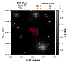
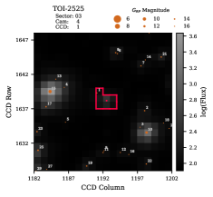
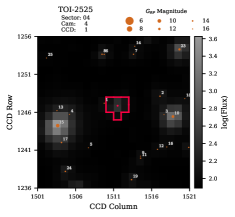
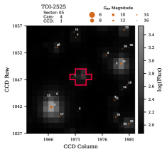
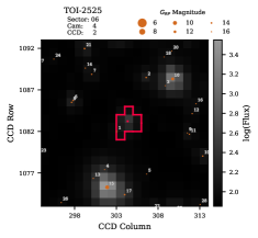
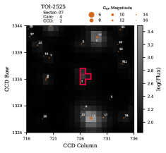
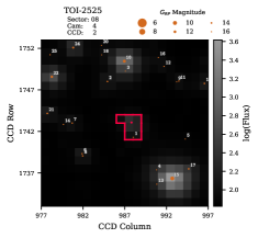
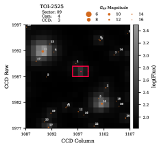
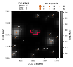
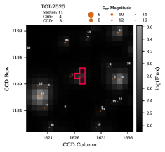
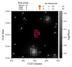
Figure 1: Target pixel file (TPF) image of TOI-2525 in the FFIs of TESS Sector 1, Sectors 3 to 11, and Sector 13. The central (red) borders in the pixel space are the ones used to construct the tesseract photometry. Gaia targets are marked with red circles, whose size has been coded by their G magnitude.

In this paper, we report the discovery of another warm massive planet pair around a K-dwarf star, which has been uncovered by TESS. This work is part of our Doppler data survey and orbital analysis efforts performed within the Warm gIaNts with tEss (WINE) collaboration, which focuses on the systematic characterization of TESS transiting warm giant planets (e.g., Brahm et al., 2019; Jordán et al., 2020; Brahm et al., 2020; Schlecker et al., 2020; Trifonov et al., 2021). We present TOI-2525 (TIC 149601126), a two-planet system, which exhibits strong transit timing variations (TTVs) of the two transiting signals detected in TESS multi-sector and ground-based photometry data. This strong TTV signal in the TOI -2525 system points to strongly interacting warm giant-mass planets close to the 2:1 mean motion resonance (MMR) commensurability.

In Sect. 2 we present the observational data used to detect and characterize the warm pair of planets orbiting TOI-2525. In Sect. 3 we introduce the stellar parameter estimates of TOI-2525. In Sect. 4 we present our orbital analysis and results, which was performed on the extracted TTVs of the planetary signals, and a self-consistent photo-dynamical modeling scheme performed jointly with the acquired Doppler data. In Sect. 4, we also provide results from an analysis on the dynamical architecture and long-term stability of the TOI-2525 system. In Sect. 5 we discuss the systems’ architecture, possible formation and evolution, and interior of the planets. Finally, in Sect. 6 we present a brief summary and our conclusions.

2 Data

Here we present the photometric light curve and Doppler data acquired for TOI-2525. The TESS space based photometry is used for transit event identification of TOI-2525 b & c, whereas additional ground based photometry was used for further TTV analysis and planetary radius estimates. Precise Doppler data were collected for further constraining the planetary masses and eccentricities, but also for the stellar parameter estimates of TOI-2525.

2.1 TESS

TOI-2525 was observed in sectors 1, 3 $-$ 11, and 13, during the first year of the TESS primary mission with a 30 minute cadence, and in sectors 27, 28, and 30 $-$ 39 with a two-minute cadence in the third mission year. TOI-2525 b and c were identified in the light curves extracted from the TESS Full Frame Images (FFIs) using the tesseract pipeline (Rojas et al. in prep.). A brief introduction of our FFI extraction with tesseract in the context of the WINE collaboration can be found in Schlecker et al. (2020), Gill et al. (2020) and Trifonov et al. (2021). Figure 1 shows the target pixel file (TPF) image of TOI-2525 constructed from the TESS FFI image frames and Gaia DR3 data (Gaia Collaboration et al., 2021). Figure 1 shows that there are no bright contaminators in the FFI aperture (red continuous contour), thus we concluded that the transit signals are indeed coming from TOI-2525 and not from neighboring stars. This was later confirmed by ground-based transit detections of TOI-2525 b, and TOI-2525 c. However, a fainter source labeled #1 is occasionally in the FFI aperture, which dilutes the FFI light curves. Since tesseract does not correct contamination in the TESS apertures from nearby stars, we follow the same methodology as used in Trifonov et al. (2021) to calculate and apply a dilution correction for the contamination of TOI-2525 on the FFI light curves.

We retrieved the two-minute cadence light-curves from the Mikulski Archive for Space Telescopes. The Science Processing Operations Center (SPOC; Jenkins et al., 2016) provides simple aperture photometry (SAP) and systematics-corrected Presearch Data Conditioning photometry (PDC, Smith et al., 2012; Stumpe et al., 2012). The PDCSAP light curves are corrected for contamination from nearby stars and instrumental systematics originating from, e.g., pointing drifts, focus changes, and thermal transients. In our work of TOI-2525, for the two-minute cadence data, we only use the corrected PDCSAP data.

2.2 ASTEP

The Antarctica Search for Transiting ExoPlanets (ASTEP, Guillot et al., 2015) instrument is a 40 cm Newton telescope installed in 2010 at the Concordia station located at $-$75.06^∘S, 123.3^∘E and an altitude of $\sim$ 3230 meters. ASTEP is a robotic telescope dedicated to photometric observations of fields of stars and their exoplanets.

Table 1: FEROS and PFS RV measurements of TOI-2525.

BJD	RV [$m\,s^{-1}$]	RVσ [$m\,s^{-1}$]	instrument
2458904.623	$-$48154.684	18.000	FEROS
2458923.562	$-$48184.684	18.100	FEROS
2459156.792	320.393	4.235	PFS
2459157.754	310.269	6.285	PFS
2459238.635	225.396	6.960	PFS
2459239.607	255.721	6.470	PFS
2459501.824	337.951	5.040	PFS
2459504.843	345.583	5.150	PFS
2459505.837	341.083	5.400	PFS
2459531.781	295.292	7.340	PFS
2459534.809	320.755	5.480	PFS

Due to the extremely low data transmission rate at the Concordia station, the data are processed automatically on-site using an IDL-based aperture photometry pipeline (Mékarnia et al., 2016). The raw light curves of up to 1 000 stars of the field are transferred to Europe on a server in Roma, Italy, and are then available for deeper analysis. These data files contain each star’s flux computed through 10 fixed circular apertures radii, so that optimal calibrated light curves can be extracted.

Thanks to the accurate TTV model prediction constructed on the TESS data, we scheduled successful observations with ASTEP on TOI-2525 b, and c. For TOI-2525 b, we detected a full transit event and a partial one on the nights UT 2021-09-17 and UT 2022-06-23, respectively, whereas for TOI-2525 c, we observed two full transit events on the nights UT 2021-04-15 and UT 2022-07-02 and two partial transit events on the nights UT 2021-06-03 and UT 2021-09-10.

2.3 Moana Observatoire Moana

A partial transit of TOI-2525 c was observed with the Siding Spring Observatory station of the Observatorie Moana telescope network (OM-SSO). OM-SSO is an RC Optical Systems RCOS20 f8.1 telescope with a focal length of 3980 mm. OM-SSO is equipped with an FLI Microline 16803 camera with 4kx4k pixels of 9 microns with a pixel scale of 0.47″and a field of view of $30\times 30\arcmin$. Observations were taken using an Astrodon Exoplanet (clear blue blocking) filter. Observations of TOI-2525 c were performed on October 29, 2021 covering an ingress. The adopted exposure time was 147 s and the airmass ranged from 1.15 to 2. OM-SSO data was processed with a dedicated automated pipeline adapted from a version that was initially developed for obtaining differential photometry of LCOGT light curves (Espinoza et al., 2019).

2.4 LCOGT

We observed one partial transit of TOI-2525 b and two partial transits of TOI-2525 c using the Las Cumbres Observatory Global Telescope (LCOGT) 1.0-m network (Brown et al., 2013) nodes at Cerro Tololo Inter-American Observatory (CTIO) and South Africa Astronomical Observatory (SAAO). The 1-m telescopes are equipped with 4096$\times$4096 SINISTRO cameras having a pixel scale of 0.389″/pixel, resulting in a Field-Of-View of 26’$\times$26’. The TOI-2525 b transit was observed from SAAO on January 11, 2022 in the Sloan-$g^{\prime}$ and Sloan-$i^{\prime}$ filters using a 4.3″ target aperture. TOI-2525 c transits were observed twice from CTIO on December 18, 2021 and February 05, 2022 in the Sloan-$g^{\prime}$ and Sloan-$i^{\prime}$ filters, respectively, using 4.0″-4.7″ target apertures. LCOGT data reduction and photometric measurements were performed using the AstroImageJ (AIJ, Collins et al., 2017) software package.

2.5 PFS

TOI-2525 was monitored with the Planet Finder Spectrograph (Crane et al., 2006, 2008, 2010) installed at the 6.5 m Magellan/Clay telescope at Las Campanas Observatory. TOI-2525 was observed with the iodine gas absorption cell of the instrument at four different observing runs between November 03, 2020, and November 16, 2021, adopting an exposure time of 1200 sec, and using a 3$\times$3 CCD binning mode to minimize read-noise. TOI-2525 was also observed without the iodine cell in order to generate the template for computing the RVs, which were derived following the methodology of Butler et al. (1996). The mean uncertainty of the PFS RVs of TOI-2525 is 5.7 m s^-1. The PFS RVs are presented in Table 1.

Table 2: Stellar parameters of TOI-2525 and their 1$\sigma$ uncertainties derived using ZASPE spectral analyses, Gaia parallax, broad band photometry and PARSEC models.

Parameter	TOI-2525	reference
Spectral type	K8V	[1]
Distance (pc)	400${}_{-2.3}^{+2.3}$	[2]
Mass ($M_{\odot}$)	0.849${}_{-0.033}^{+0.024}$ (0.042)	This paper
Radius ($R_{\odot}$)	0.785${}_{-0.007}^{+0.007}$ (0.031)	This paper
Luminosity ($L{{}_{\odot}}$)	0.363${}_{-0.016}^{+0.016}$ (0.008)	This paper
Age (Gyr)	3.99${}_{-2.60}^{+4.30}$	This paper
AV (mag)	0.287${}_{-0.074}^{+0.070}$	This paper
$T_{\mathrm{eff}}$ (K)	5096 $\pm$ 80 (102)	This paper
$\log g\leavevmode\nobreak\ [\mathrm{cm\cdot s}^{-2}]$	4.58 $\pm$ 0.20	This paper
[Fe/H]	0.14 $\pm$ 0.05	This paper
$v\cdot\sin(i)$ (km s-1)	1.5 $\pm$ 0.3	This paper

2.6 FEROS

We obtained three Doppler measurements of TOI-2525 with the FEROS spectrograph (Kaufer et al., 1999) installed at the MPG 2.2 m telescope in La Silla Observatory. These spectra were taken on BJD = 2458904.623, 2458914.612, 2458923.562, with the simultaneous ThAr wavelength calibration technique. The exposure times were set to 1800 seconds, yielding an average signal-to-noise ratio of 25. The FEROS data were reduced, extracted and analyzed with the ceres pipeline (Brahm et al., 2017a) delivering radial velocity and bisector span measurements with a mean uncertainty of 19 m s^-1. The RV datum obtained on BJD = 2458914.612, however, was a clear outlier with a poor accuracy due to bad weather conditions. Therefore, we could rely on only two FEROS spectra, which are fully consistent with the orbital fit to the TTVs and the PFS data. However, the two FEROS RVs have no effective weight on the orbital fit, since their contribution is canceled by the two additional fitting parameters RV${}_{\rm off.\leavevmode\nobreak\ FEROS}$ and RV${}_{\rm jit.\leavevmode\nobreak\ FEROS}$. Thus, we decided to not use the FEROS RVs in our orbital analysis. The obtained FEROS radial velocities are presented in Table 1.

3 Stellar parameters of TOI-2525

TOI-2525 is an early K-type star visible in the southern hemisphere. The star has a distance of $400.0\pm 2.3$ pc from the Sun and an apparent magnitude of $13.4$ mag in the TESS bandpass. The atmospheric and physical parameters were obtained using three co-added FEROS spectra and the ZASPE code (Brahm et al., 2017b). This code compares the stellar spectra with synthetic atmospheric models generated from the ATLAS9 model atmospheres (Castelli & Kurucz, 2004). The result is generated using the $\chi^{2}$ method at regions in the spectra which are most sensitive to changes. Parameters obtained from these regions are calculated iteratively. The errors of the values are generated with Monte Carlo simulations for the depth of the spectral lines. For TOI-2525, an effective temperature of $T_{\rm eff}=5096\pm 80$ K, a metallicity of $[{\text{Fe/H}}]=0.14\pm 0.05$ dex, with respect to the solar metallicity, and a projected rotational velocity of $v\text{sin}i=1.5\pm 0.3$ km sec^-1 were calculated.

Table 3: Planetary radii, orbital inclinations, and stellar density and mass estimates of the TOI-2525 system, derived during TTV extraction.

Parameter	median	$\sigma$
$r_{b}$ (RJup.)	0.88	0.02
$r_{c}$ (RJup.)	0.98	0.02
$i_{b}$ (deg)	89.31	0.03
$i_{c}$ (deg)	89.96	0.03
$\rho_{\star}$ (gr cm${}^{-3})$	2.14	0.04
$M_{\star}$ ($M_{\odot}$)	0.85	0.05

The physical parameters are estimated as in Brahm et al. (2020). We used the PARSEC stellar isochrones (Bressan et al., 2012), which contain the absolute magnitudes of several band passes for a set of ages, masses, and metallicities. Since the latter were already calculated in the first step, they are fixed in the subsequent iteration. Using the spectroscopic temperatures, the Gaia parallaxes, and the observed magnitudes, the age and the mass were obtained via a Markov Chain Monte Carlo (MCMC) exploration of the parameter space by using the emcee package (Foreman-Mackey et al., 2013). The result is an age of $3.99^{+4.3}_{-2.6}$ G yr, a mass of $\text{M}_{\star}=0.849^{+0.024}_{-0.033}\,\text{M}_{\sun}$ and a radius of $\text{R}_{\star}=0.785\pm 0.007\,\text{R}_{\sun}$. Our relatively small uncertainties in the ZASPE stellar parameters, however, are internal and do not include possible systematic differences with respect to other stellar models. Therefore, we followed the prescription of Tayar et al. (2022) who suggest systematic uncertainty floor of order $\sim$5% in mass, $\sim$4% in radius and $\sim$2% in temperature and luminosity, respectively (see, Tayar et al., 2022, for more details). We adopt these relative uncertainties to access more realistic stellar parameter errors through this work. The full set of atmospheric and physical parameters are listed in Table 2.

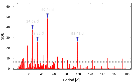
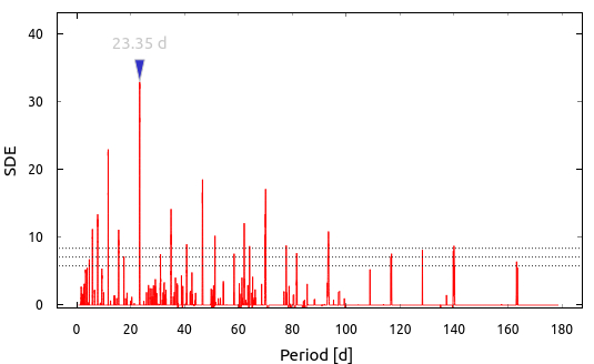
Figure 2: The top panel shows the TLS power spectra of the detrended TESS FFI light curve data of TOI-2525. The planetary transit signal of the more massive planet c is detected at $P_{c}=49.24$ d. The bottom panel shows the TLS power spectra of the residuals, which reveal the transit signal of the inner less-massive planet at $P_{b}=23.3$ d. The remaining TLS peaks are harmonics and sub-harmonics of the transit signals. Horizontal dashed lines indicate the signal detection efficiency (SDE; Hippke et al., 2019) power level of 5.7, 7.0, and 8.3, which correspond to the TLS false positive rate of 10%,1%, and 0.1%.

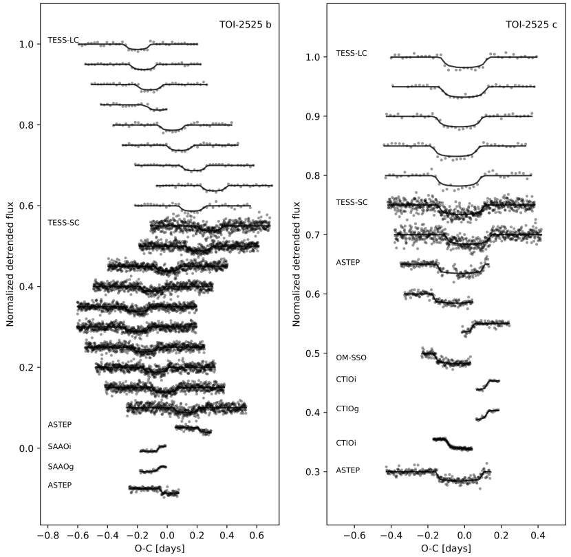
Figure 3: TESS light-curve data and model of the TOI-2525 transit signals, plotted with arbitrary vertical offsets. The left panel shows the transit signal of the inner planet TOI-2525 b and its strong TTV variation, whereas the right panel shows the same for the outer, more massive Jovian planet TOI-2525 c. The x-axis of the curves for TOI-2525 b is $t_{\rm n}$-1333.5070$\bmod$23.2915 days, and for TOI-2525 c is $t_{\rm n}$-1335.4101$\bmod$49.2424 days, respectively.

4 Analysis and results

4.1 Preliminary data vetting

We identify the transit events of TOI-2525 b & c in the first-year TESS FFI light curves. Our preliminary transit characterization methodology includes detrending of the tesseract FFI light curves with a robust (iterative) Matérn GP kernel via the wotan package (see Hippke et al., 2019) and a transit signal search with the transitleastsquares (TLS; Hippke & Heller, 2019) algorithm.

Fig. 2 shows our TLS results on the combined TESS FFI light curve data of TOI-2525. We first detect the stronger transit signal of TOI-2525 c with a period of $\approx$ 49.3 d. We filter this signal by applying a Keplerian transit model with the obtained parameters from the TLS, and we seek additional transit signals in the model residuals. We clearly find the shallower, but more frequent, transit signal of the inner planet TOI-2525 b at a period of $P_{b}=23.3$ d. Fig. 2 shows many other significant TLS peaks with a signal detection efficiency (SED, see, Hippke & Heller, 2019)) of $>$ 8.3, which are nothing more than the integer sub-harmonics of the transit signals.

From the FFI data, we found that the light curve mid-transit time of TOI-2525 b and TOI-2525 c are not linear in time and show strong deviations in the expected time-of-transits, i.e., TTVs.

The available Doppler data of TOI-2525 are too few for an independent RV validation of the two-planet system (see Table 1). Since we identified the transit events in 2019, we have made many attempts to collect precise spectroscopic data from the southern hemisphere. However, TOI-2525 is faint and requires significant observational efforts and excellent sky conditions. This, in combination with the COVID-19 pandemic closures of the ESO and Las Campanas observatories, prevented us from obtaining sufficient RV data. Nonetheless, we conclude that at this point, the PFS data alone are adequate for validation of the system when combined with the transit periods from TESS, and can contribute to the planetary mass estimates when combined with the strong TTVs.

$\begin{array}[]{ccc}\includegraphics[width=253.22934pt]{TTV_model_planet1_sep22.jpg}\hskip 5.69046pt\includegraphics[width=253.22934pt]{TTV_model_planet2_sep22.jpg}\\ \end{array}$

Figure 4: TTVs of TOI-2525 b (blue) and TOI-2525 c (red), fitted with a two-planet dynamical model jointly with the RVs from PFS. The top panels show the TTVs time series and best-fit model for each planet, whereas the bottom panels show the TTVs residuals.

4.1.1 Extraction of TTVs

Transit timing variations were estimated by fitting all the available photometric data using the exoplanet software package (Foreman-Mackey et al., 2021). We used the descriptive model TTVOrbit which assumes Keplerian orbits for each planet but allows for the central time of each transit to be a free parameter in the model. The parameters of the model are the values of $R_{p}$ for each planet, their impact parameters $b$, the transit times, the stellar mass $M_{\star}$ and density $\rho_{\star}$, quadratic limb darkening coefficients $u_{1}$ and $u_{2}$ for each instrument used, and parameters to describe trends and correlations in the data. Regarding the latter, we adopt a linear model in time for the ground based transits, which are often only partially observed, and a Gaussian process (GP) for each of the short and long cadence TESS datasets. The Gaussian process kernel adopted is a damped simple harmonic oscillator (Foreman-Mackey et al., 2017a) with $Q=1/3$, variance $\sigma_{\rm GP}$ and correlation length parameter $\rho_{\rm GP}$.

Table 3 lists the resulting light curve parameters, whereas Fig. 3 shows the resulting light curve models applied to all photometric data sets. Both TOI-2525 transit signals exhibit strong TTV libration. The values of the fitted transit times for each transit are listed in Table A2.

$\begin{array}[]{ccc}\includegraphics[width=170.71652pt]{RV_model_sep22.jpg}\hskip 1.42271pt\includegraphics[width=170.71652pt]{RV_model_sep22_ph_pl1.jpg}\hskip 1.42271pt\includegraphics[width=170.71652pt]{RV_model_sep22_ph_pl2.jpg}\\ \end{array}$

Figure 5: RV component of the two-planet dynamical model of TOI-2525, constructed jointly with the TTVs data and with the RVs from PFS (blue circles). The two RVs from FEROS (red triangles) are overploted with an optimized RV offset to the model. The left panel shows the time series and the N-body model, the middle and right panels show a phase-folded representation of the RV data, modeled with the dynamical model (with an osculating period). The PFS data uncertainties include the estimated RV jitter, added in quadrature to the error budget, while the FEROS data are plotted with their nominal RV uncertainties. The small sub-panels show the RVs residuals.

4.2 Orbital analysis

4.2.1 Joint RV and TTV analysis

For the joint RV and TTV orbital analysis of the TOI-2525 system, we followed a similar route to the one we used in Trifonov et al. (2021) for the modeling of the TOI-2022 system. We refer the reader to that paper for a more detailed description of the chosen methodology. Briefly, for TOI-2525 we performed orbital fitting with the Exo-Striker exoplanet toolbox (Trifonov, 2019) by adopting the self-consistent dynamical model on the extracted TTVs from Sect. 4.1.1. The TTV model can provide a relatively inexpensive orbital and dynamical solution to the system, in terms of CPU-time. However, it also comes with a severe ambiguity in eccentricity versus dynamical planetary-mass (e.g., Lithwick et al., 2012; Dawson et al., 2021a; Trifonov et al., 2021). Therefore, we fit the TTVs jointly with the RV data from PFS to better constrain the planetary dynamical masses and eccentricities. The RV model is intrinsic to Exo-Striker, whereas the TTV model is wrapped around the TTVfast package (Deck et al., 2014). The fitted parameters for each planet were the RV semi-amplitude $K$ (which is automatically converted to the dynamical planetary mass $m_{p}$), orbital period $P$, eccentricity $e$, argument of periastron $\omega$, and mean anomaly $M_{0}$. Our TTVs+RVs modelling scheme allows a difference in the planetary inclinations ($\Delta i$ $\geq$ 0^∘). Thus, we also model the orbital inclinations $i$ and the difference between the line of node $\Delta\Omega$. All these parameters are valid for BJD = 2458333.52, which is an arbitrarily epoch, chosen slightly before the first transit event of the inner planet. The RV data offset and jitter parameters of PFS added two more free parameters.

Finally, our dynamical model, particularly the planetary masses, also depends on the stellar mass estimate of TOI-2525, for which we adopt a fixed value of 0.849 $M_{\odot}$. We set the time step in the dynamical model to $dt$ = 0.02 days to assure sufficient orbital resolution and accuracy.

Table 4: Nested sampling priors, posteriors, and the optimum $-\ln\mathcal{L}$ orbital parameters of the two-planet system TOI-2525 derived by joint dynamical modeling of TTVs (TESS, ASTEP, SSO, and LCOGT) and radial velocities (FEROS, PFS).

Median and $1\sigma$               Max. $-\ln\mathcal{L}$                            Adopted priors
Parameter	Planet b	Planet c		Planet b	Planet c		Planet b	Planet c
$K$ [m s-1]	7.1${}_{-0.3}^{+0.3}$	44.4${}_{-1.5}^{+1.5}$		7.1	44.4		$\mathcal{U}$(5.0,30.00)	$\mathcal{U}$(20.0,60.0)
$P$ [day]	23.288${}_{-0.002}^{+0.001}$	49.260${}_{-0.001}^{+0.001}$		23.289	49.260		$\mathcal{U}$(23.2,23.4)	$\mathcal{U}$(49.1,49.4)
$e$	0.159${}_{-0.007}^{+0.012}$	0.152${}_{-0.005}^{+0.006}$		0.171	0.160		$\mathcal{U}$(0.0,0.4)	$\mathcal{U}$(0.0,0.4)
$\omega$ [deg]	346.3${}_{-0.7}^{+0.7}$	21.8${}_{-0.8}^{+0.8}$		346.5	22.0		$\mathcal{U}$(0.0,360.0)	$\mathcal{U}$(0.0,360.0)
$M_{\rm 0}$ [deg]	120.8${}_{-0.5}^{+0.6}$	71.2${}_{-1.0}^{+1.2}$		120.6	71.6		$\mathcal{U}$(0.0,360.00)	$\mathcal{U}$(0.0,360.00)
$\lambda$ [deg]	107.0${}_{-0.8}^{+0.8}$	93.4${}_{-1.0}^{+0.9}$		107.1	93.1		(derived)	(derived)
$i$ [deg]	89.96${}_{-0.07}^{+0.08}$	89.99${}_{-0.06}^{+0.08}$		89.97	89.99		$\mathcal{N}$(90.0,0.1)	$\mathcal{N}$(90.0,0.1)
$\Omega$ [deg]	0.0	2.0${}_{-1.2}^{+1.9}$		0.0	1.9		(fixed)	$\mathcal{N}$(0.0,15.0)
$\Delta i$ [deg]	2.0${}_{-1.2}^{+1.9}$	$\dots$		1.9	$\dots$		(derived)	$\dots$
$a$ [au]	0.1511${}_{-0.0025}^{+0.0025}$	0.2491${}_{-0.0042}^{+0.0041}$		0.1511	0.2491		(derived)	(derived)
$m$ [$M_{\rm jup}$]	0.088${}_{-0.004}^{+0.005}$	0.709${}_{-0.034}^{+0.034}$		0.089	0.710		(derived)	(derived)
$\rho$ [g cm-3]	0.174${}_{-0.015}^{+0.016}$	1.014${}_{-0.076}^{+0.084}$		0.174	1.014		(derived)	(derived)
RVoff. PFS [m s-1]	$-$28.5${}_{-7.4}^{+7.1}$	$\dots$		$-$32.2	$\dots$		$\mathcal{U}$(-300.00,100.0)	$\dots$
RVjit. PFS [m s-1]	26.8${}_{-5.4}^{+6.8}$	$\dots$		21.5	$\dots$		$\mathcal{J}$(0.0,50.0)	$\dots$

We ran a nested sampling (NS) scheme (Skilling, 2004), which allowed us to efficiently explore the complex parameter space of osculating orbital elements and study the parameter posteriors and overall dynamics. Our NS run was performed with the dynesty sampler (Speagle, 2020), which is integrated into Exo-Striker. We ran 100 "live-points" per fitted parameter using the "Dynamic" NS scheme, focused on 100% posterior convergence instead of log-evidence (see, Speagle, 2020, for details) Parameter priors were estimated by running several experimental NS runs and adopting a wide range of uniform parameter priors. After a few consecutive NS runs, we narrowed the adequate parameter space to be explored. We note that we adopted very narrow priors on the orbital inclinations to assure the TTV+RV model parameter space is consistent with the inclination estimates extracted from the TTVs. Thus, we eliminate configurations that could explain the RV data but would not lead to transit events (i.e., impact parameters $b_{\rm b}$ and $b_{\rm c}$, which are inconsistent with the light curve signal). The final adopted parameter priors are listed in Table 4.

Fig. 4 and Fig. 5 show the TTVs and RVs data together with the best-fit joint dynamical model of TOI-2525. The left and the right panels of Fig. 4 show the TTVs of TOI-2525 b & c, respectively, fitted with the best-fit TTV model. Fig. 5 shows the RV component of the best-fit model applied to the PSF RVs. In Fig. 5 also shows the two FEROS RVs fitted independently to the best-fit with an optimized offset. The middle and the right panel of Fig. 5 show a phase-folded representation of the RV signals of TOI-2525 b & c, respectively, modeled with an osculating period. The signal of the inner planet TOI-2525 b is strongly overshadowed by the dominating signal of the outer one due to the large difference in K amplitudes (see Table 4).

The final posterior probability distributions with an RV linear trend are shown in Fig. A1. Our final estimates for TOI-2525 b & c lead to planetary orbital periods of P_b = 23.288${}_{-0.002}^{+0.001}$ days, and P_c = 49.260${}_{-0.001}^{+0.001}$ days, eccentricities of $e_{b}$ = 0.159${}_{-0.007}^{+0.012}$ and $e_{c}$ = 0.152${}_{-0.005}^{+0.006}$, and dynamical masses of $m_{b}$ = 0.088${}_{-0.004}^{+0.005}$ $M_{\rm jup}$ and $m_{c}$ = 0.709${}_{-0.034}^{+0.034}$ $M_{\rm jup}$. The mutual inclination is constrained to $\Delta i$ = 2.0${}_{-1.2}^{+1.9}$ deg. Given the planetary radii obtained during the TTV extraction in Sect. 4.1.1, we derive a remarkably low density of $\rho_{b}$=0.174${}_{-0.015}^{+0.016}$ g cm^-3 for the inner planet, and $\rho_{c}$=1.014${}_{-0.076}^{+0.084}$ g cm^-3, for the outer one, respectively. The full list of posterior and maximum $-\ln\mathcal{L}$ (i.e., best-fit) estimates was derived from the joint TTVs+RVs model and listed in Table 4.

$\begin{array}[]{ccc}\includegraphics[width=455.24408pt]{out_TOI2525_TTVs_dynNS_SEP_22_4_out_1a.pdf}\par\par\par\end{array}$

Figure 6: Posteriors of the dynamical properties at the 2:1 period ratio commensurability of the two-planet system TOI-2525. The posteriors are generated by randomly drawing 10 000 samples from the TTV+RV dynamical model. Each sample is tested for stability and the overall dynamical properties are evaluated at the 2:1 period ratio commensurability. The derived dynamical parameters are: mean period ratio $\hat{P}_{\rm rat.}$, mean eccentricities $\hat{e}_{\rm b}$, $\hat{e}_{\rm c}$, mean orbital aligment $\hat{\Delta\omega}$, and their peak-to-peak amplitudes Ampl. $e_{\rm b}$, Ampl. $e_{\rm c}$, Ampl. $\Delta\omega$, and the planetary dynamical masses and semi-major axes. Note that the posterior distribution of $\theta_{1}$, and $\theta_{2}$ are not shown, since these exhibit circulation between 0^∘ and 360^∘. The black contours on the 2D panels represent the 1, 2 and 3$\sigma$ confidence level of the overall posterior samples.

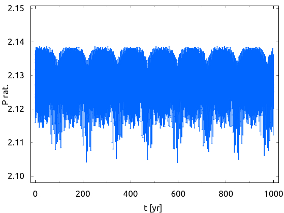
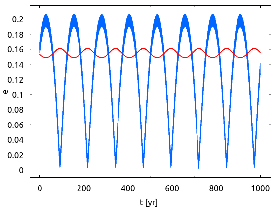
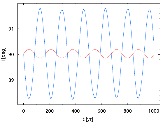
Figure 7: Orbital evolution of the TOI-2525 system for a 1 000 yr long N-body integration using the Wisdom-Holman scheme. The left panel shows the evolution of the planetary periods, the middle panel shows the eccentricities $e_{\rm b}$ (blue) and $e_{\rm c}$ (red) of the best-fit N-body model, while the right panel shows the evolution of the line-of-sight inclinations $i_{\rm b}$ (blue) and $i_{\rm c}$ (red).

4.2.2 Joint RV and photodynamical analysis

A complementary analysis of the light curves and RVs of TOI-2525 was performed using the flexi-fit python package. For modeling the photometric data, flexi-fit employs analytic transit light curves (Mandel & Agol, 2002) with a quadratic limb-darkening. Dynamical effects are included via the rebound $N$-body package (Rein & Liu, 2012). Our orbital analysis with flexi-fit is performed in Jacobi-coordinates using the ias15 integrator (Everhart, 1985), which automatically determines the numerical time step $dt$ down to machine precision. The fitting with flexi-fit relies on a Markov Chain Monte Carlo (MCMC) parameter sampling provided by the emcee sampler (Foreman-Mackey et al., 2013), which converges to the posterior probability distribution.

The flexi-fit model provides orbital parameters valid for the epoch BJD = 2458333.52, which is the same as the one chosen for joint TTVs + RVs analysis (see Sect. 4.1.1). We chose uniform parameter priors which define an equal probability of occurrence between predefined borders. Most of the priors were generously defined, covering a large section of parameter space. The only priors worth mentioning are for the periods $P_{b}\in\mathcal{U}$(23.1,23.4), $P_{c}\in\mathcal{U}$(49.1,49.4) days which is sufficient considering the mid-transit times and the inclination $i_{b}\in\mathcal{U}$(81,99), $i_{c}\in\mathcal{U}$(81,99) degrees, which can be restricted to these intervals for geometrical reasons, because we do observe transits. The remaining priors of the photodynamical model are listed in Table A3. Having the stellar parameters (Table 2) and quadratic limb-darkening coefficients given, our free orbital parameters for each planet are the orbital period $P$, the mass $m$, the eccentricity $e$, the longitude of periastron $\omega$, the time of first conjunction with respect to the start of integration $t_{conj}$, the inclination $i$ and the planet to star radius ratio $R_{p}/R_{s}$. The longitude of the ascending node $\Omega$ was fixed $\Omega_{b}=0$ for the inner planet and free for the outer planet. For the instrumental and observational errors from the radial velocity data from PFS, a jitter parameter and an offset were determined.

The photometric data were separated into 8 distinct data sets: TESS FFIs (year 1), TESS PDC (year 3), ASTEP 1-6, CTIO, SSO and SAAO 1-2. The photometric data from the TESS-FFIs in the first TESS-year were de-trended sector-wise using the rspline in the wotan package (Hippke et al., 2019) package. For the third year of the TESS observations, the 2-min cadence data from the PDCSAP pipeline, as well as the ground based photometry data from ASTEP, CTIO, SSO and SAAO were included into the model without further de-trending. For each data set, an offset was fitted. In total, this adds up to 30 dimensions of fitting, all the other parameters including the RV semi-amplitude $K$ are derived.

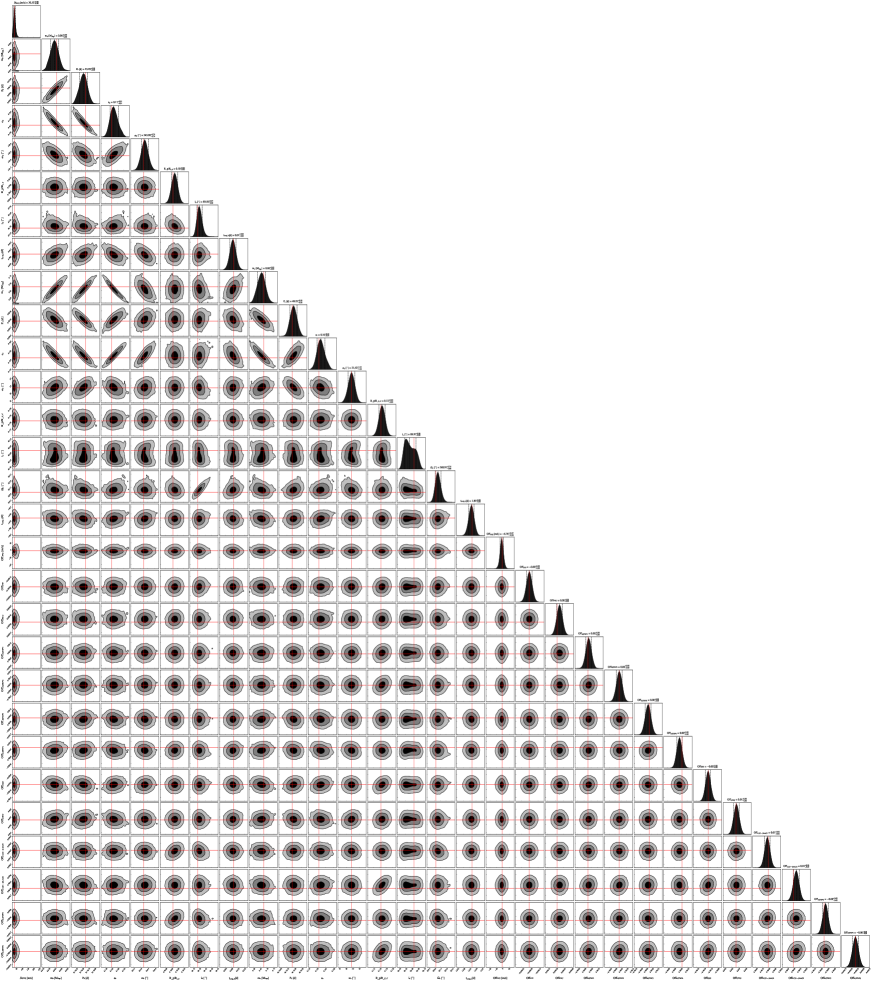
Figure A4: Posterior distribution for the joint photodynamical analysis. The orbital parameters of both planets and jitter and offset terms are obtained by an MCMC analysis in flexi-fit https://gitlab.gwdg.de/sdreizl/exoplanet-flexi-fit. The best-fit posteriors are marked in red. The scattered black lines represent the median and the $1\sigma$ intervals of the distribution.

Fig. A2 and Fig. A3 show an impression of the light curves for TESS FFI, TESS PDC, ASTEP, and SSO, fitted jointly with flexi-fit. The posterior distributions of the MCMC can be seen in Fig. A4. Both masses $m_{b}=0.084_{-0.005}^{+0.005}\mathrm{M_{Jup}}$ and $m_{c}=0.657_{-0.032}^{+0.031}\mathrm{M_{Jup}}$ were estimated to an error of less than 10%. Combined with the planetary radii of $R_{b}=0.774_{-0.010}^{+0.010}R_{Jup}$ and $R_{c}=0.904_{-0.010}^{+0.010}R_{Jup}$ we got a very low density of $\rho_{b}=0.226_{-0.014}^{+0.015}$ g cm^-3 for the inner planet. The density for the outer planet is $\rho_{c}=1.11_{-0.07}^{+0.07}$ g cm^-3. The planetary densities are slightly larger than our results from the TTVS+RV analysis. The orbital parameters, offsets, and jitter parameters from the photodynamical orbital analysis are listed in Table A3.

Here we note that applying a photodynamical model on a system having RV data and large photometric data sets (of the order 200 000 data points) for more than $1000\leavevmode\nobreak\ \mathrm{d}$ is computationally expensive. On a standard CPU, an iteration of the MCMC takes approximately $2.5\leavevmode\nobreak\ \mathrm{s}$, which keeps the length of the chain limited. Since the analysis was very time-consuming, the analysis was stopped after 100 000 MCMC iterations. The convergence criterion of 20 % mean acceptance fraction was not reached (see, Foreman-Mackey et al., 2013), but the physical and dynamical parameters correspond to those from the light curve and RV+TTV analysis presented in Sect. 4.1.1 and Sect. 4.2.1 and give us confidence in our orbital solution.

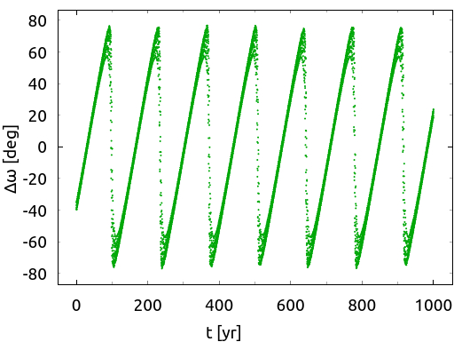
Figure 8: The top panels; a) and b) show the same as in Fig. 7, but for the evolution of the apsidal angle $\Delta\omega$ = $\omega_{\rm b}$ - $\omega_{\rm c}$, and the trajectory evolution as a function $e_{b}e_{c}$ times sine/cosine of $\Delta\omega$, respectively. The trajectory just misses the origin (red dot, centred at [0,0]), which leads to libration of $\Delta\omega$ with a semi-amplitude of $\sim$ 80^∘. The bottom panels c) and d) show the same as in a) and b), but for a random posterior fit which exhibits circulation of $\Delta\omega$ (see Fig. 6). The trajectory evolution in this case passes through the origin, which leads to brief episodes of circulation of $\Delta\omega$.

4.3 Dynamics and long-term stability

Following Trifonov et al. (2021), we inspected the Hill (see, Gladman, 1993) and Angular Momentum Deficit (AMD, see, Laskar & Petit, 2017) stability criteria of the TOI-2525 system. In terms of the classical Hill stability criterion, the TOI-2525 planetary system is predicted to be stable. We estimate a mutual Hill distance of $\sim$ 7.4 R_Hill,m, which is above the widely accepted distance of $\sim$ 3.5 R_Hill,m for the system to be considered Hill-stable. However, accounting for the estimated orbital eccentricities, semi-major axes, mutual orbital inclination, and planetary masses of TOI-2525 b & c, the AMD criterion suggests that the TOI-2525 planetary system is unstable. The AMD criterion is very sensitive to eccentricities. Thus, the moderately eccentric orbits of the pair are the reason for the negative AMD result.

As discussed in Trifonov et al. (2021), the AMD and Hill stability criteria are only a proxy for long-term stability and do not account for the system’s dynamics near mean motion resonances. Therefore, to test the long-term dynamics and possible MMR in the system, we adopt exactly the same $N$-body numerical setup used in our recent analysis of TOI-2202 (Trifonov et al., 2021). This is adequate because TOI-2202 and TOI-2525 share somewhat similar physical and orbital characteristics. We refer the reader to Section 5 in Trifonov et al. (2021) for more details about the stability test performed here for TOI-2525. Briefly, we performed numerical integrations using a custom version of the Wisdom-Holman $N$-body algorithm (Wisdom & Holman, 1991), which directly adopts and integrates the Jacobi orbital elements from the posterior orbital analysis. We test the stability of the TOI-2525 system up to 1 Myr with a small time-step of 0.02  d for 10 000 randomly chosen samples from the achieved orbital parameter posteriors from the TTV+RV dynamical modelling scheme. We automatically monitored the evolution of the planetary semi-major axes, eccentricities, secular apsidal angle $\Delta\omega$ = $\omega_{\rm b}$ - $\omega_{\rm c}$, and first-order 2:1 MMR angles $\theta_{1}=\lambda_{\rm b}-2\lambda_{\rm c}+\omega_{\rm b},\leavevmode\nobreak\ \leavevmode\nobreak\ \theta_{2}=\lambda_{\rm b}-2\lambda_{\rm c}+\omega_{\rm c}$ (where $\lambda_{\rm b,c}$ = $M_{\rm b,c}$ + $\omega_{\rm b,c}$ is the mean longitude of planet b and c, respectively; see Lee, 2004). These angles are important for libration in secular apsidal alignment or mean motion resonance.

We found that all examined 10 000 samples are stable for 1 Myr. Fig. 6 presents the resulted posterior probability distribution of some of the important dynamical properties of the system, such as mean period ratio $P_{\rm rat.}$, mean eccentricities $\hat{e}_{\rm b}$, $\hat{e}_{\rm c}$, their peak-to-peak amplitudes Ampl. $e_{\rm b}$, Ampl. $e_{\rm c}$, dynamical masses of the planets $m_{\rm b}$, $m_{\rm c}$, and the orbital semi-major axes $a_{\rm b}$, $a_{\rm c}$. Fig. 6 shows that the period ratio evolution is bimodal, oscillating either around $\sim$ 2.127, or more plausibly around $\sim$ 2.126, which are too far from the exact 2:1 period ratio for the system to librate in the 2:1 MMR. This is confirmed by the circulation of $\theta_{1}$ and $\theta_{2}$, which distributions are not shown in Fig. 6. On the other hand, we observe a bi-modality of the evolution of $\Delta\omega$, which is intriguing. About half of the sampled initial conditions lead to libration of $\Delta\omega$ about $0^{\circ}$ with a mean semi-amplitude around 80^∘, whereas the rest of the sampled initial conditions seem to exhibit a mean semi-amplitude around $180^{\circ}$, i.e., circulation (see Sect. 5.1 for more explanation on this dynamical behavior).

Fig. 7 shows an example of a 1000 yr extent of the orbital evolution simulation started from the best-fit (i.e., maximum $-\ln\mathcal{L}$, see Table 4). We show the evolution of the eccentricities, mutual period ratio $P_{\rm rat.}$ the eccentricities $e_{\rm b}$ and $e_{\rm c}$, and the orbital inclinations $i_{\rm b}$ and $i_{\rm c}$. The TOI-2525 system is consistent with moderate eccentricity evolution, and appears to osculate outside of the low-order eccentricity-type 2:1 MMR. It is interesting that the secular evolution time scales are rather short, of the order of $\sim$ 120 yr. Therefore, future observations might be sensitive to transit depth variations. Furthermore, TOI-2525 b may soon become a non-transiting planet (different timescales are possible within the mutually inclined posteriors).

5 Discussion

5.1 Dynamical state of the system

Our numerical orbital analysis of the system’s configuration revealed that the TOI-2525 pair of planets are outside of the 2:1 MMR. However, the posterior of the apsidal alignment angle $\Delta\omega$ shows bi-modality with approximately equal fraction exhibiting libration and circulation. Thus, we took a closer look at the dynamical evolution of these two populations. The upper and lower panels of Fig. 8 show the characteristic evolution of $\Delta\omega$ for the same stable configuration as in Fig. 7 (i.e., our best TTV+RV fit) and for a random posterior fit with $\Delta\omega$ in circulation, respectively. The left panels of Fig. 8 show $\Delta\omega$ as a function of time, whereas the right panels show the trajectory in the polar plot of $e_{b}e_{c}\cos\Delta\omega$ vs $e_{b}e_{c}\sin\Delta\omega$. In both cases, the polar plot shows that the system circulates around a point along the positive $e_{b}e_{c}\cos\Delta\omega$ axis, i.e., an aligned configuration. For the best fit shown in the upper panels, the trajectory in the polar plot is just small enough to miss the origin, and $\Delta\omega$ exhibits large amplitude libration about $0^{\circ}$. For the example shown in the lower panels, the trajectory in the polar plot is just large enough to touch the origin, which leads to brief episodes of circulation of $\Delta\omega$. Thus, the bi-modality of the apsidal alignment angle is simply due to slightly different sizes of the trajectories in the secular polar variables.

$\begin{array}[]{ccc}\includegraphics[width=247.53888pt]{toi2525_cut.pdf}\\ \end{array}$

Figure 9: The 2:1 MMR structure diagram following Nesvorný & Vokrouhlický (2016). Four planetary systems are plotted: TOI-2525 (this work), TOI-2202 (Trifonov et al., 2021), TOI-216 (Dawson et al., 2021b) and Kepler-88 (Nesvorný et al., 2013). The separatrices and stable point are solid. The dotted line is an approximation of the stable point inside the resonance, as explained in Nesvorný & Vokrouhlický (2016). The dashed line is the unstable point. Dot-dashed is the stable point. See Nesvorný & Vokrouhlický (2016) for more explanations.

$\begin{array}[]{ccc}\includegraphics[width=256.0748pt,height=184.9429pt]{RaMa_Teq.jpg}\put(-215.0,165.0){a)}\includegraphics[width=256.0748pt,height=184.9429pt]{RaMa_pho.jpg}\put(-215.0,165.0){b)}\\ \end{array}$

Figure 10: Radius-mass demographics for all giant transiting planets with measured masses by TTVs or RVs. The position of TOI-2525 b and c are plotted with "star" symbols. Panel a) shows the mass-radius relation color-coded by T_eq.. Panel b) shows the same as panel a), but is color-coded with the planetary density. The solid curve corresponds to the predicted radius using the models of Fortney et al. (2007) given the estimated luminosity of TOI-2525, a semi-major axis=0.2 AU, and an age of 3.1 G yr.

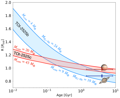
Figure 11: Evolution models of TOI-2525 b and TOI-2525 c. All models assume a central ice-rock core surrounded by a hydrogen-helium envelope of solar composition. For both planets, the range of core masses is shown. For TOI-2525 b, the range of envelope masses is also shown. The errorbars correspond to observational constraints on their age and radius, compared to the ones of Jupiter and Saturn.

We ruled out a 2:1 MMR librating configuration of the system based on the orbital posterior probability distribution constructed from the available transit and RV data. Similarly to the TOI-2202 system, the osculating period ratio of the TOI-2525 pair of planets is well above two, consistent with the prominent peak of period ratios of planet pairs observed by the Kepler mission (Lissauer et al., 2011; Fabrycky et al., 2014). Fig. 9 shows an analytical analysis of the resonant and near-resonant dynamics in the 2:1 commensurability, following Nesvorný & Vokrouhlický (2016). The constant $\delta$ is an orbital invariant that defines the position of the system relative to the 2:1 period ratio, $\psi$ is a combination of the resonant angles $\theta_{1}$ and $\theta_{2}$, whereas the variable $\Psi$ is a combination of planetary masses, semi-major axes and eccentricities (see, Nesvorný & Vokrouhlický, 2016, for details). Fig. 9 is an updated version of Figure 12 in Trifonov et al. (2021), which now includes the position of TOI-2525, in addition to TOI-2202 Trifonov et al. (2021), TOI-216 (Dawson et al., 2021b) and Kepler-88 (Nesvorný et al., 2013). The median posterior probability values of TOI-2525, listed in Table 4, lead to $\delta\simeq$ -1.60, therefore, firmly outside the libration region together with Kepler-88 and TOI-2525 systems. The only system that is in a 2:1 MMRs is TOI-216 (see, Dawson et al., 2021b, for details).

5.2 Possible formation mechanisms

An interesting question is how frequently state-of-the-art planet formation models produce systems like TOI-2525, TOI-2202, or TOI-216 and what drives their formation. We explored the abundance and origins of systems with multiple giant planets in synthetic planet populations from the Generation III Bern model (Emsenhuber et al., 2021a, b; Schlecker et al., 2021a, b; Burn et al., 2021; Mishra et al., 2021). The model includes the mechanisms relevant for the dynamical evolution of multi-planet systems, in particular type I and type II planet migration (Paardekooper et al., 2011; Dittkrist et al., 2014), eccentricity and inclination damping through planet-disk interaction (Cresswell & Nelson, 2008), and dynamical evolution modeled via an N-body integrator (Chambers, 1999). The planet population with 0.7 $M_{\odot}$ host star mass introduced in Burn et al. (2021) is most suitable for the comparison with the K dwarf system presented here. Out of its 999 systems, 92 contain planets more massive than 30 $M_{\oplus}$. We find 51 systems with more than one such planet within orbital periods of 1000  d in the population, typically around host stars with enhanced metallicity. Only a single system includes a pair of warm giant planets in an MMR-like configuration: It contains three giant planets with periods of $48.0\,\mathrm{d}$, $96.5\,\mathrm{d}$, and $479.8\,\mathrm{d}$.

The system emerged from a numerical disk with a large solid material content, which is reflected in a high dust-to-gas ratio of 0.024 as compared to the population median of 0.014. This led to efficient core growth and runaway gas accretion of three protoplanets. Through simultaneous inward migration and gravitational interaction, the two warm gas giants were eventually captured in an MMR, a configuration that persisted until the end of the N-body integration at 20 Myr. This comparison proposes that the TOI-2525 system was formed in a similar metal-enriched disk. TOI-2525 is thus in a configuration whose realization through core accretion is rare but possible, according to the simulations.

We note that the literature contains other examples of pairs of warm Jovian planets that have been extensively studied. For instance, the Kepler-9 system, consisting of a G-dwarf star orbited by a mini-Saturn planet pair in a 2:1 MMR (Holman et al., 2010). Other examples include the HD 82943 Tan et al. (2013) and TIC 279401253 (Bozhilov et al., submitted) systems, both of which are G-dwarf stars with almost identical 2:1 MMR Jovian-mass planet pairs. Although rare, M-dwarfs have also been found to host 2:1 MMR warm massive systems, with the GJ 876 multiple planet system (Rivera et al., 2010; Millholland et al., 2018; Trifonov et al., 2018), being widely considered as a benchmark for planetary dynamics and planet formation. The formation of such systems may not depend on the stellar type, but its occurrence rate remains an important observable to be further studied.

5.3 TOI-2525 b; a very low-density planet

TOI-2525 b and c are two warm low-density giant planets, a category of planetary systems whose frequency is steadily growing in the literature. The estimated mean density of TOI-2525 c of $\rho_{\rm c}$ = 1.014${}_{-0.076}^{+0.084}$ g cm^-3 is lower than that of Jupiter ($\rho_{\rm Jup.}$ = 1.33 g cm^-3), but is higher than that of Saturn ($\rho_{\rm Sat.}$ = 0.69 g cm^-3). Therefore, the density of the Jovian mass planet TOI-2525 c is not surprising. The Neptune-mass planet TOI-2525 b, however, has a mean density of $\rho_{\rm b}$ = 0.174${}_{-0.015}^{+0.016}$ g cm^-3, which makes it among the lowest density Neptune-mass planets known to date. The density of TOI-2525 b is a bit larger than the Kepler-51 b, c, and d ‘‘super puffs’’ (Steffen et al., 2013; Masuda, 2014), and is comparable to low-density planets like WASP-107 b (Rubenzahl et al., 2021), WASP-131 b, WASP-139 b (Hellier et al., 2017), WASP-21 b (Barros et al., 2011; Ciceri et al., 2013), HATS-46b b (Brahm et al., 2018), among others. We use the mass-radius models by Fortney et al. (2007) to infer the core mass of the TOI-2525 b and c planets given the estimated masses, radii, and stellar parameters. We calculate core masses of 6.9 $\pm$ 1.4 $M_{\oplus}$ and 36.6 $\pm$ 9.3 $M_{\oplus}$, for TOI-2525 b and TOI-2525 c, respectively. The ratio of core-mass to the total mass $Zp$, is therefore; $Zp_{b}$ = 0.25 $\pm$ 0.05, and $Zp_{c}$ = 0.17 $\pm$ 0.04.

Fig. 10 shows a mass-radius plot for all known transiting planets with measured masses validated by TTVs or RVs. Fig. 10 is limited only to the giant planets in the range of 0.05 to 11 $M_{\rm Jup.}$, and 0.15 to 3.0 $R_{\rm Jup.}$. Panel a) of Fig. 10 is color-coded with the planetary equilibrium temperature (T_eq.), whereas panel b) is color-coded with the planetary density. In both panels, we plot an interpolated model for the mass-radius relationship assuming the estimated luminosity of TOI-2525, semi-major axis=0.2 AU, and age of 3.1 G yr from Fortney et al. (2007). From Fig. 10 it is clear that the higher T_eq. of the planet, the larger the radius is. Except for the massive planets with few Jupiter masses and more, the larger radius correlates with low planetary density. TOI-2525 c is consistent with the mass-radius model from Fortney et al. (2007). TOI-2525 b is consistent with a large radius, and its mean density is among the lowest for the Neptune-mass planets.

We also model the evolution of both planets in the system, using CEPAM (Guillot & Morel, 1995; Guillot et al., 2006) and a non-grey atmosphere (Parmentier et al., 2015), to provide constraints on their interior. We assume simple structures consisting of a central dense core surrounded by a hydrogen and helium envelope of solar composition. The core is assumed made with 50% of ices and 50% of rocks. Fig. 11 shows the resulting evolution models. The core mass of TOI-2525 c is found to be between 20 and 43  $M_{\oplus}$. This indicates that the enrichment in heavy elements of TOI-2525 c could be comparable to Jupiter’s, which is between 8 and 46 $M_{\oplus}$ (Guillot et al., 2022). With a radius almost similar to Saturn’s (1.08 times larger) but 3.4 times less massive than Saturn, TOI-2525 b is an uncommon example of very low-density and inflated planet with an equilibrium temperature close to 500 K. The H-He envelope of TOI-2525 b is found to be between 19 and 24 $M_{\oplus}$. The case of TOI-2525 b is challenging for the traditional core-accretion formation scenario. With our simple modeling of TOI-2525 b, a such small envelope hints that the accretion of H-He have potentially been hindered. Characterizing the atmospheres of both planets of the system would be very useful to understand their structure and formation.

Not many inflated Neptune-mass planets are known, making TOI-2525 b a useful addition to the sample of transiting planets with a measured mass. The low-density, and thus, large scale-height of TOI-2525 b makes it a good target for a future atmospheric investigation with transmission spectroscopy.

6 Summary and Conclusions

We report the discovery of a warm pair of giant planets around a K-dwarf star, uncovered by TESS with multi-sector light curve photometry. The TOI-2525 light curve shows recurrent transit events consistent with two gravitationally interacting giant planets, resulting in a robust TTVs signal with a semi-amplitude of $\sim$6 hours for the inner planet. We obtained precise spectroscopic Doppler follow-up with the FEROS and the PFS spectrographs to estimate the stellar parameters and constrain the planetary masses. Using high signal-to-noise FEROS spectra of TOI-2525, we estimate a stellar mass of M_⋆ = 0.849${}_{-0.033}^{+0.024}$ M_⊙ and a stellar radius of R_⋆ = 0.785${}_{-0.007}^{+0.007}$ R_⊙. Using these stellar mass and radius, we conducted an extensive orbital analysis of the TESS TTVs and RVs using self-consistent N-body models. This analysis allowed us to construct an accurate orbital model from which we predicted future transit events, confirmed by follow-up photometry observations by ASTEP, OM-SSO, and LCOGT.

The complete collection of RVs and transit light curves allowed us to perform more extensive joint TTV+RV analyses, as well as light curve photodynamical+RV N-body orbital modeling. We found that TOI-2525 b is a massive-Neptune with a dynamical mass of m_b = 0.088${}_{-0.005}^{+0.005}$ $M_{\rm jup}$, and radius of $R_{\rm b}$ = 0.88${}_{-0.02}^{+0.02}$ $R_{\rm jup}$. Thus, the estimated density of TOI-2525 b is $\rho_{\rm b}$ = 0.174${}_{-0.015}^{+0.016}$ g cm^-3, which makes it among the lowest density Neptune-mass planets known to date, similar to the Kepler 51 planets. The outer transiting planet TOI-2525 c is a Jovian-mass planet with $m_{\rm c}$ = 0.709${}_{-0.034}^{+0.034}$ $M_{\rm jup}$, and planetary radius $R_{\rm c}$ =0.98${}_{-0.02}^{+0.02}$ $R_{\rm jup}$, and therefore, with a relatively low mean density of $\rho_{\rm c}$ = 1.014${}_{-0.076}^{+0.084}$ g cm^-3.

The warm pair of massive planets is near the 2:1 period ratio commensurability with orbital periods of $P_{\rm b}$ = 23.288${}_{-0.002}^{+0.001}$ d and $P_{\rm c}$ = 49.260${}_{-0.001}^{+0.001}$ d, but the dynamics of the system clearly suggest that it is outside the mean motion resonance (MMR) dynamical configuration.

The TOI-2525 system is very similar to other K-dwarf TESS systems; TOI-2202 and TOI-216 are composed of almost identical K dwarf primary and two warm giant planets near the 2:1 MMR. These three systems will be a useful sample for studying the formation and composition of warm giant pairs around K-dwarf stars.

In this Appendix, we show in Table A2 we list the estimated mid-transit time estimates of TOI-2525 b and c (i.e., TTVs), in Table A3 we list the estimated posterior probability distribution of our joint Doppler and transit light curve photodynamical model with flexifit, in Fig. A1 shows the posterior probability distribution of the joint Doppler and TTV modeling with Exo-Striker, in Fig. A2 and Fig. A3 we show the flexifit model applied to the available transit lightcurves, and finally, in Fig. A4 we show the MCMC posterior probability distribution of the flexifit joint photodynamical analysis.

$\begin{array}[]{ccc}\includegraphics[width=512.1496pt]{TOI2525_TTVs_lintr_dynNS_SEP_22_4_final.pdf}\end{array}$

Figure A1: Exo-Striker global parameters search results of the TESS, the ASTEP, the OM-SSO, and the LCOGT TTVs, of TOI-2525 b and TOI-2525 c, and the Doppler radial velocities from FEROS and PFS. The posterior probability distribution is acheaved with a nested sampling scheme employing a two-planet self-consistent dynamical model. The black contours on the 2D panels represent the 1, 2, and 3$\sigma$ confidence level of the overall posteriors. Red crosses point to the median position of the posterior parameters.

Table A1: Parameters of the two-planet system TOI-2525, its host star and the light curves derived during TTV extraction (continues from Table 3).

Parameter	median	$\sigma$
$\mu_{\rm TESS-LC}$	$-$0.0003	0.0004
$\log(\rho)_{\rm TESS-LC}$	0.830	0.093
$\log(\sigma)_{\rm TESS-LC}$	$-$5.628	0.056
$\mu_{\rm TESS-SC}$	0.0000	0.0001
$\log(\rho)_{\rm TESS-SC}$	0.526	0.156
$\log(\sigma)_{\rm TESS-SC}$	$-$7.246	0.058
$\mu_{\rm ASTEP1}$	0.0002	0.0001
$\beta_{\rm ASTEP1}$	0.0054	0.002
$\mu_{\rm ASTEP2}$	0.0000	0.0001
$\beta_{\rm ASTEP2}$	-0.001	0.002
$\mu_{\rm ASTEP3}$	0.0000	0.0002
$\beta_{\rm ASTEP3}$	$-$0.005	0.005
$\mu_{\rm ASTEP4}$	0.0006	0.0002
$\beta_{\rm ASTEP4}$	0.0185	0.005
$\mu_{\rm ASTEP5}$	$-$0.0001	0.0001
$\beta_{\rm ASTEP5}$	$-$0.004	0.002
$\mu_{\rm ASTEP6}$	$-$0.0001	0.0001
$\beta_{\rm ASTEP6}$	$-$0.004	0.0008
$\mu_{\rm SSO}$	$-$0.0007	0.0003
$\beta_{\rm SSO}$	$-$0.008	0 006
$\mu_{\rm CTIOi}$	0.0030	0.0002
$\beta_{\rm CTIOi}$	$-$0.0061	0.0081
$\mu_{\rm CTIOg}$	0.0031	0.0002
$\beta_{\rm CTIOg}$	$-$0.0404	0.0105
$\mu_{\rm CTIOi2}$	0.0047	0.0001
$\beta_{\rm CTIOi2}$	$-$0.0024	0.0039
$u_{0,\rm TESS}$	0.502	0.150
$u_{1,\rm TESS}$	0.422	0.189
$u_{0,\rm ASTEP}$	0.409	0.072
$u_{1,\rm ASTEP}$	$-$0.159	0.069
$u_{0,\rm SSO}$	0.528	0.220
$u_{1,\rm SSO}$	0.053	0.299
$u_{0,\rm SAAO,g}$	0.688	0.330
$u_{1,\rm SAAO,g}$	$-$0.055	0.348
$u_{0,\rm SAAO,i}$	0.403	0.143
$u_{1,\rm SAAO,i}$	0.057	0.220

Table A2: Individual mid-transit time estimates of TOI-2525 b extracted from TESS, ASTEP, SSO and LCOGT used for TTV analysis.

N Transit	t0 [BJD]	$\sigma$ t0 [BJD]	Instrument
	Planet b
1	2458333.527	0.005	TESS
4	2458403.441	0.002	TESS
5	2458426.775	0.007	TESS
6	2458450.130	0.011	TESS
7	2458473.508	0.008	TESS
8	2458496.853	0.003	TESS
9	2458520.237	0.004	TESS
11	2458566.956	0.002	TESS
15	2458659.976	0.009	TESS
32	2459056.051	0.006	TESS
33	2459079.266	0.003	TESS
35	2459125.641	0.003	TESS
36	2459148.834	0.003	TESS
38	2459195.308	0.004	TESS
39	2459218.599	0.004	TESS
41	2459265.237	0.003	TESS
42	2459288.598	0.003	TESS
43	2459311.952	0.003	TESS
45	2459358.682	0.004	TESS
50	2459475.305	0.004	ASTEP
55	2459591.328	0.002	LCOGT-SAAO
	Planet c
1	2458335.410	0.004	TESS
2	2458384.648	0.002	TESS
3	2458433.866	0.006	TESS
4	2458483.090	0.007	TESS
8	2458680.073	0.005	TESS
17	2459123.270	0.003	TESS
19	2459221.791	0.003	TESS
21	2459320.238	0.002	ASTEP
22	2459369.454	0.003	ASTEP
24	2459467.906	0.003	ASTEP
25	2459517.190	0.003	SSO

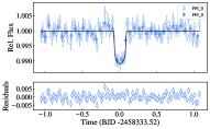
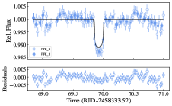
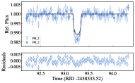
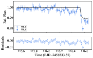
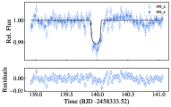
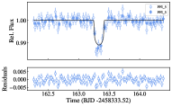
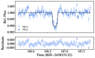
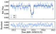
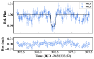
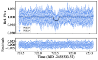
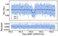
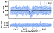
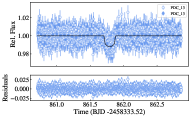
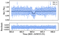
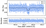
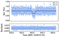
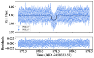
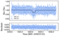
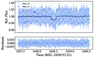
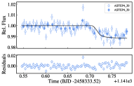
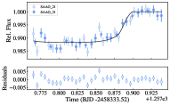
Figure A2: Shown are all Transit lightcurves of TOI-2525b from the photodynamic model observed by different telescopes. Nine of them are TESS observed (FFI), eleven are TESS observed transits (PDCSAP), two transits are observed by ASTEP, and one by SAAO. A 30-minute binning was introduced after the fit with errors calculated by standard deviation (filled circles).

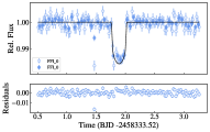
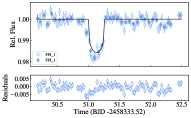
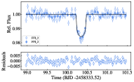
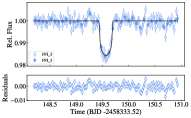
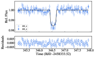
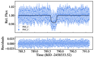
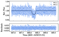
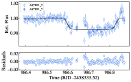
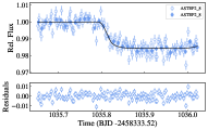
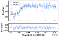
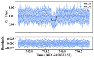
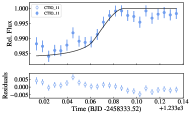
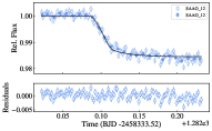
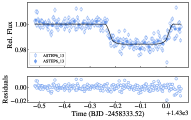
Figure A3: Shown are all Transit lightcurves of TOI-2525c from the photodynamic model observed by different telescopes. Five of them are TESS observed (FFI), three are TESS observed transits (PDCSAP), four transits are observed by ASTEP, one by CTIO and one by SAAO. A 30-minute binning was introduced after the fit with errors calculated by standard deviation (filled circles).

Table A3: MCMC posterior medians, best-fits and adopted priors from orbital elements, offset and jitter terms from flexi-fit.

Parameter	median and $1\sigma$	best-fit	adopted prior
TOI-2525b
period $P$ [d]	$23.2856_{-0.0017}^{+0.0017}$	$23.2865$	$\mathcal{U}$(23.1,23.4)
mass $m$ [$\mathrm{M_{Jup}}$]	$0.084_{-0.005}^{+0.005}$	$0.086$	$\mathcal{U}$(10,100 M⊕)
eccentricity $e$	$0.170_{-0.010}^{+0.011}$	$0.167$	$\mathcal{U}$(0,0.45)
longitude of periastron $\omega$[∘]	$345.9_{-0.8}^{+0.8}$	$345.7$	$\mathcal{U}$(0,360)
time of conjunction $t_{conj}$ [BJD-2457000d]	$1333.5289_{-0.0020}^{+0.0020}$	$1333.5293$	$\mathcal{U}$(1333.52,1356.82)
inclination $i$ [∘]	$89.50_{-0.07}^{+0.07}$	$89.47$	$\mathcal{U}$(80,100)
planet to star radius ratio $R_{p}/R_{s}$	$0.1013_{-0.0008}^{+0.0008}$	$0.1009$	$\mathcal{U}$(0.001,0.2)
longitude of ascending node $\Omega$[∘]	$0$ (fixed)	$0$ (fixed)	(fixed)
radius $R_{p}$ [$R_{Jup}$]	$0.774_{-0.010}^{+0.010}$	$0.771$	(derived)
density $\rho$ [$\mathrm{g/cm^{3}}$]	$0.225_{-0.014}^{+0.015}$	$0.235$	(derived)
semi-major axis $a$ [au]	$0.1511_{-0.0020}^{+0.0020}$	$0.1511$	(derived)
transit duration $t_{dur}$[h]	$4.05_{-0.07}^{+0.07}$	$4.00$	(derived)
RV semi-amplitude $K$ [m/s]	$6.7_{-0.4}^{+0.4}$	$6.9$	(derived)
mean longitude $\lambda$ [∘]	$107.8_{-0.8}^{+0.8}$	$107.5$	(derived)
TOI-2525c
period $P$ [d]	$49.2519_{-0.0004}^{+0.0004}$	$49.2518$	$\mathcal{U}$(49.1,49.4)
mass $m$ [$\mathrm{M_{Jup}}$]	$0.657_{-0.032}^{+0.031}$	$0.675$	$\mathcal{U}$(100,400 M⊕)
eccentricity $e$	$0.157_{-0.007}^{+0.008}$	$0.153$	$\mathcal{U}$(0,0.45)
longitude of periastron $\omega$[∘]	$21.5_{-1.1}^{+1.1}$	$21.5$	$\mathcal{U}$(0,360)
time of conjunction $t_{conj}$ [BJD-2457000d]	$1335.4118_{-0.0014}^{+0.0014}$	$1335.4121$	$\mathcal{U}$(1333.52,1382.77)
inclination $i$ [∘]	$89.97_{-0.07}^{+0.09}$	$90.03$	$\mathcal{U}$(80,100)
planet to star radius ratio $R_{p}/R_{s}$	$0.1183_{-0.0005}^{+0.0005}$	$0.1182$	$\mathcal{U}$(0.001,0.25)
longitude of ascending node $\Omega$[∘]	$1.1_{-0.7}^{+1.0}$	$0.4$	$\mathcal{U}$(-10,10)
radius $R_{p}$ [$R_{Jup}$]	$0.904_{-0.010}^{+0.010}$	$0.903$	(derived)
density $\rho$ [$\mathrm{g/cm^{3}}$]	$1.11_{-0.07}^{+0.07}$	$1.14$	(derived)
semi-major axis $a$ [au]	$0.249_{-0.004}^{+0.004}$	$0.249$	(derived)
transit duration $t_{dur}$[h]	$5.502_{-0.027}^{+0.013}$	$5.514$	(derived)
RV semi-amplitude $K$ [m/s]	$41.2_{-2.2}^{+2.2}$	$42.2$	(derived)
mean longitude $\lambda$ [∘]	$93.2_{-1.1}^{+1.1}$	$93.2$	(derived)
$\mathrm{RV_{off}}$ PFS [m/s]	$-7_{-11}^{+11}$	$-4$	$\mathcal{U}(-\infty,\infty)$
$\mathrm{RV_{jit}}$ PFS [m/s]	$31_{-7}^{+10}$	$29$	$\mathcal{U}(exp(-5),exp(5))$
$\mathrm{TR_{off}}$ TESS FFI [ppm]	$-310_{-60}^{+60}$	$-300$	$\mathcal{U}(-\infty,\infty)$
$\mathrm{TR_{off}}$ TESS PDC (year 3) [ppm]	$380_{-60}^{+60}$	$330$	$\mathcal{U}(-\infty,\infty)$
$\mathrm{TR_{off}}$ ASTEP 1 [ppm]	$390_{-260}^{+250}$	$320$	$\mathcal{U}(-\infty,\infty)$
$\mathrm{TR_{off}}$ ASTEP 2 [ppm]	$350_{-260}^{+260}$	$340$	$\mathcal{U}(-\infty,\infty)$
$\mathrm{TR_{off}}$ ASTEP 3 [ppm]	$210_{-320}^{+310}$	$340$	$\mathcal{U}(-\infty,\infty)$
$\mathrm{TR_{off}}$ ASTEP 4 [ppm]	$650_{-330}^{+320}$	$940$	$\mathcal{U}(-\infty,\infty)$
$\mathrm{TR_{off}}$ SSO [ppm]	$-1870_{-310}^{+310}$	$-1850$	$\mathcal{U}(-\infty,\infty)$
$\mathrm{TR_{off}}$ CTIO [ppm]	$6690_{-410}^{+410}$	$6620$	$\mathcal{U}(-\infty,\infty)$
$\mathrm{TR_{off}}$ SAAO1 [ppm]	$7880_{-350}^{+350}$	$8000$	$\mathcal{U}(-\infty,\infty)$
$\mathrm{TR_{off}}$ SAAO2 [ppm]	$9140_{-150}^{+150}$	$9000$	$\mathcal{U}(-\infty,\infty)$
$\mathrm{TR_{off}}$ ASTEP5 [ppm]	$-500_{-170}^{+160}$	$-580$	$\mathcal{U}(-\infty,\infty)$
$\mathrm{TR_{off}}$ ASTEP6 [ppm]	$-280_{-130}^{+130}$	$-270$	$\mathcal{U}(-\infty,\infty)$

References

- Astropy Collaboration et al. (2013) Astropy Collaboration, Robitaille, T. P., Tollerud, E. J., et al. 2013, A&A, 558, A33, doi: 10.1051/0004-6361/201322068
- Astropy Collaboration et al. (2018) Astropy Collaboration, Price-Whelan, A. M., Sipőcz, B. M., et al. 2018, AJ, 156, 123, doi: 10.3847/1538-3881/aabc4f
- Baluev (2009) Baluev, R. V. 2009, MNRAS, 393, 969, doi: 10.1111/j.1365-2966.2008.14217.x
- Barros et al. (2011) Barros, S. C. C., Pollacco, D. L., Gibson, N. P., et al. 2011, MNRAS, 416, 2593, doi: 10.1111/j.1365-2966.2011.19210.x
- Baruteau et al. (2014) Baruteau, C., Crida, A., Paardekooper, S. J., et al. 2014, in Protostars and Planets VI, ed. H. Beuther, R. S. Klessen, C. P. Dullemond, & T. Henning, 667, doi: 10.2458/azu_uapress_9780816531240-ch029
- Bitsch et al. (2020) Bitsch, B., Trifonov, T., & Izidoro, A. 2020, A&A, 643, A66, doi: 10.1051/0004-6361/202038856
- Brahm et al. (2017a) Brahm, R., Jordán, A., & Espinoza, N. 2017a, PASP, 129, 034002, doi: 10.1088/1538-3873/aa5455
- Brahm et al. (2017b) Brahm, R., Jordán, A., Hartman, J., & Bakos, G. 2017b, MNRAS, 467, 971, doi: 10.1093/mnras/stx144
- Brahm et al. (2018) Brahm, R., Hartman, J. D., Jordán, A., et al. 2018, AJ, 155, 112, doi: 10.3847/1538-3881/aaa898
- Brahm et al. (2019) Brahm, R., Espinoza, N., Jordán, A., et al. 2019, AJ, 158, 45, doi: 10.3847/1538-3881/ab279a
- Brahm et al. (2020) Brahm, R., Nielsen, L. D., Wittenmyer, R. A., et al. 2020, The Astronomical Journal, 160, 235, doi: 10.3847/1538-3881/abba3b
- Brasseur et al. (2019) Brasseur, C. E., Phillip, C., Fleming, S. W., Mullally, S. E., & White, R. L. 2019, Astrocut: Tools for creating cutouts of TESS images. http://ascl.net/1905.007
- Bressan et al. (2012) Bressan, A., Marigo, P., Girardi, L., et al. 2012, MNRAS, 427, 127, doi: 10.1111/j.1365-2966.2012.21948.x
- Brown et al. (2013) Brown, T. M., Baliber, N., Bianco, F. B., et al. 2013, PASP, 125, 1031, doi: 10.1086/673168
- Burn et al. (2021) Burn, R., Schlecker, M., Mordasini, C., et al. 2021, Astronomy & Astrophysics, 656, A72, doi: 10.1051/0004-6361/202140390
- Butler et al. (1996) Butler, R. P., Marcy, G. W., Williams, E., et al. 1996, PASP, 108, 500, doi: 10.1086/133755
- Castelli & Kurucz (2004) Castelli, F., & Kurucz, R. L. 2004, Astronomy and Astrophysics, 405, 1095, doi: 10.1051/0004-6361:20030619
- Chambers (1999) Chambers, J. E. 1999, MNRAS, 304, 793, doi: 10.1046/j.1365-8711.1999.02379.x
- Ciceri et al. (2013) Ciceri, S., Mancini, L., Southworth, J., et al. 2013, A&A, 557, A30, doi: 10.1051/0004-6361/201321669
- Coleman & Nelson (2014) Coleman, G. A. L., & Nelson, R. P. 2014, MNRAS, 445, 479, doi: 10.1093/mnras/stu1715
- Collins et al. (2017) Collins, K. A., Kielkopf, J. F., Stassun, K. G., & Hessman, F. V. 2017, AJ, 153, 77, doi: 10.3847/1538-3881/153/2/77
- Crane et al. (2006) Crane, J. D., Shectman, S. A., & Butler, R. P. 2006, in Proc. SPIE, Vol. 6269, Society of Photo-Optical Instrumentation Engineers (SPIE) Conference Series, 626931, doi: 10.1117/12.672339
- Crane et al. (2010) Crane, J. D., Shectman, S. A., Butler, R. P., et al. 2010, in Proc. SPIE, Vol. 7735, Ground-based and Airborne Instrumentation for Astronomy III, 773553, doi: 10.1117/12.857792
- Crane et al. (2008) Crane, J. D., Shectman, S. A., Butler, R. P., Thompson, I. B., & Burley, G. S. 2008, in Proc. SPIE, Vol. 7014, Ground-based and Airborne Instrumentation for Astronomy II, 701479, doi: 10.1117/12.789637
- Cresswell & Nelson (2008) Cresswell, P., & Nelson, R. P. 2008, A&A, 482, 677, doi: 10.1051/0004-6361:20079178
- Dawson et al. (2021a) Dawson, R. I., Huang, C. X., Brahm, R., et al. 2021a, AJ, 161, 161, doi: 10.3847/1538-3881/abd8d0
- Dawson et al. (2021b) —. 2021b, arXiv e-prints, arXiv:2102.06754. https://arxiv.org/abs/2102.06754
- Deck et al. (2014) Deck, K. M., Agol, E., Holman, M. J., & Nesvorný, D. 2014, ApJ, 787, 132, doi: 10.1088/0004-637X/787/2/132
- Dittkrist et al. (2014) Dittkrist, K. M., Mordasini, C., Klahr, H., Alibert, Y., & Henning, T. 2014, Astronomy and Astrophysics, 567, doi: 10.1051/0004-6361/201322506
- Dong et al. (2021) Dong, J., Huang, C. X., Dawson, R. I., et al. 2021, ApJS, 255, 6, doi: 10.3847/1538-4365/abf73c
- Dumusque et al. (2019) Dumusque, X., Turner, O., Dorn, C., et al. 2019, A&A, 627, A43, doi: 10.1051/0004-6361/201935457
- Emsenhuber et al. (2021a) Emsenhuber, A., Mordasini, C., Burn, R., et al. 2021a, Astronomy & Astrophysics, 656, A69, doi: 10.1051/0004-6361/202038553
- Emsenhuber et al. (2021b) —. 2021b, Astronomy & Astrophysics, 656, A70, doi: 10.1051/0004-6361/202038863
- ESA (1997) ESA, ed. 1997, ESA Special Publication, Vol. 1200, The HIPPARCOS and TYCHO catalogues. Astrometric and photometric star catalogues derived from the ESA HIPPARCOS Space Astrometry Mission
- Espinoza et al. (2019) Espinoza, N., Hartman, J. D., Bakos, G. Á., et al. 2019, AJ, 158, 63, doi: 10.3847/1538-3881/ab26bb
- Espinoza et al. (2020) Espinoza, N., Brahm, R., Henning, T., et al. 2020, MNRAS, 491, 2982, doi: 10.1093/mnras/stz3150
- Everhart (1985) Everhart, E. 1985, in Astrophysics and Space Science Library, Vol. 115, IAU Colloq. 83: Dynamics of Comets: Their Origin and Evolution, ed. A. Carusi & G. B. Valsecchi, 185, doi: 10.1007/978-94-009-5400-7_17
- Fabrycky & Tremaine (2007) Fabrycky, D., & Tremaine, S. 2007, ApJ, 669, 1298, doi: 10.1086/521702
- Fabrycky et al. (2014) Fabrycky, D. C., Lissauer, J. J., Ragozzine, D., et al. 2014, ApJ, 790, 146, doi: 10.1088/0004-637X/790/2/146
- Foreman-Mackey (2016) Foreman-Mackey, D. 2016, The Journal of Open Source Software, 1, 24, doi: 10.21105/joss.00024
- Foreman-Mackey (2018) Foreman-Mackey, D. 2018, Research Notes of the American Astronomical Society, 2, 31, doi: 10.3847/2515-5172/aaaf6c
- Foreman-Mackey et al. (2017a) Foreman-Mackey, D., Agol, E., Ambikasaran, S., & Angus, R. 2017a, AJ, 154, 220, doi: 10.3847/1538-3881/aa9332
- Foreman-Mackey et al. (2017b) Foreman-Mackey, D., Agol, E., Angus, R., & Ambikasaran, S. 2017b, AJ, 154, 220, doi: 10.3847/1538-3881/aa9332
- Foreman-Mackey et al. (2013) Foreman-Mackey, D., Hogg, D. W., Lang, D., & Goodman, J. 2013, PASP, 125, 306, doi: 10.1086/670067
- Foreman-Mackey et al. (2021) Foreman-Mackey, D., Luger, R., Agol, E., et al. 2021, The Journal of Open Source Software, 6, 3285, doi: 10.21105/joss.03285
- Foreman-Mackey et al. (2021) Foreman-Mackey, D., Savel, A., Luger, R., et al. 2021, exoplanet-dev/exoplanet v0.5.1, doi: 10.5281/zenodo.1998447
- Fortney et al. (2007) Fortney, J. J., Marley, M. S., & Barnes, J. W. 2007, ApJ, 659, 1661, doi: 10.1086/512120
- Francesco et al. (2022) Francesco, A., Mario, D., Li, Z., & Alessandro, S. 2022, Research Notes of the American Astronomical Society, 6, 28, doi: 10.3847/2515-5172/ac52f2
- Gaia Collaboration et al. (2016) Gaia Collaboration, Prusti, T., de Bruijne, J. H. J., et al. 2016, A&A, 595, A1, doi: 10.1051/0004-6361/201629272
- Gaia Collaboration et al. (2018) Gaia Collaboration, Brown, A. G. A., Vallenari, A., et al. 2018, A&A, 616, A1, doi: 10.1051/0004-6361/201833051
- Gaia Collaboration et al. (2021) —. 2021, A&A, 649, A1, doi: 10.1051/0004-6361/202039657
- Gill et al. (2020) Gill, S., Wheatley, P. J., Cooke, B. F., et al. 2020, ApJ, 898, L11, doi: 10.3847/2041-8213/ab9eb9
- Gladman (1993) Gladman, B. 1993, Icarus, 106, 247, doi: 10.1006/icar.1993.1169
- Goldreich & Tremaine (1979) Goldreich, P., & Tremaine, S. 1979, The Astrophysical Journal, 233, 857
- Guerrero et al. (2021) Guerrero, N. M., Seager, S., Huang, C. X., et al. 2021, ApJS, 254, 39, doi: 10.3847/1538-4365/abefe1
- Guillot et al. (2022) Guillot, T., Fletcher, L. N., Helled, R., et al. 2022, arXiv e-prints, arXiv:2205.04100. https://arxiv.org/abs/2205.04100
- Guillot & Morel (1995) Guillot, T., & Morel, P. 1995, A&AS, 109, 109
- Guillot et al. (2006) Guillot, T., Santos, N. C., Pont, F., et al. 2006, A&A, 453, L21, doi: 10.1051/0004-6361:20065476
- Guillot et al. (2015) Guillot, T., Abe, L., Agabi, A., et al. 2015, Astronomische Nachrichten, 336, 638, doi: 10.1002/asna.201512174
- Hellier et al. (2017) Hellier, C., Anderson, D. R., Collier Cameron, A., et al. 2017, MNRAS, 465, 3693, doi: 10.1093/mnras/stw3005
- Hippke et al. (2019) Hippke, M., David, T. J., Mulders, G. D., & Heller, R. 2019, AJ, 158, 143, doi: 10.3847/1538-3881/ab3984
- Hippke & Heller (2019) Hippke, M., & Heller, R. 2019, A&A, 623, A39, doi: 10.1051/0004-6361/201834672
- Holman et al. (2010) Holman, M. J., Fabrycky, D. C., Ragozzine, D., et al. 2010, Science, 330, 51, doi: 10.1126/science.1195778
- Huang et al. (2016) Huang, C., Wu, Y., & Triaud, A. H. M. J. 2016, ApJ, 825, 98, doi: 10.3847/0004-637X/825/2/98
- Ida & Lin (2010) Ida, S., & Lin, D. N. C. 2010, ApJ, 719, 810, doi: 10.1088/0004-637X/719/1/810
- Jenkins et al. (2016) Jenkins, J. M., Twicken, J. D., McCauliff, S., et al. 2016, in Proc. SPIE, Vol. 9913, Software and Cyberinfrastructure for Astronomy IV, 99133E, doi: 10.1117/12.2233418
- Jordán et al. (2020) Jordán, A., Brahm, R., Espinoza, N., et al. 2020, AJ, 159, 145, doi: 10.3847/1538-3881/ab6f67
- Kanagawa et al. (2018) Kanagawa, K. D., Tanaka, H., & Szuszkiewicz, E. 2018, ApJ, 861, 140, doi: 10.3847/1538-4357/aac8d9
- Kaufer et al. (1999) Kaufer, A., Stahl, O., Tubbesing, S., et al. 1999, The Messenger, 95, 8
- Kipping (2013) Kipping, D. M. 2013, MNRAS, 435, 2152, doi: 10.1093/mnras/stt1435
- Kley & Nelson (2012) Kley, W., & Nelson, R. P. 2012, ARA&A, 50, 211, doi: 10.1146/annurev-astro-081811-125523
- Kossakowski et al. (2019) Kossakowski, D., Espinoza, N., Brahm, R., et al. 2019, MNRAS, 490, 1094, doi: 10.1093/mnras/stz2433
- Kreidberg (2015) Kreidberg, L. 2015, PASP, 127, 1161, doi: 10.1086/683602
- Kumar et al. (2019) Kumar, R., Carroll, C., Hartikainen, A., & Martin, O. A. 2019, The Journal of Open Source Software, doi: 10.21105/joss.01143
- Laskar & Petit (2017) Laskar, J., & Petit, A. C. 2017, A&A, 605, A72, doi: 10.1051/0004-6361/201630022
- Lee (2004) Lee, M. H. 2004, ApJ, 611, 517, doi: 10.1086/422166
- Levison et al. (2015) Levison, H. F., Kretke, K. A., & Duncan, M. J. 2015, Nature, 524, 322, doi: 10.1038/nature14675
- Lightkurve Collaboration et al. (2018) Lightkurve Collaboration, Cardoso, J. V. d. M., Hedges, C., et al. 2018, Lightkurve: Kepler and TESS time series analysis in Python, Astrophysics Source Code Library. http://ascl.net/1812.013
- Lin & Papaloizou (1979) Lin, D. N. C., & Papaloizou, J. 1979, Monthly Notices of the Royal Astronomical Society, 186, 799, doi: 10.1093/mnras/186.4.799
- Lin & Papaloizou (1986) Lin, D. N. C., & Papaloizou, J. 1986, ApJ, 309, 846, doi: 10.1086/164653
- Lissauer et al. (2011) Lissauer, J. J., Ragozzine, D., Fabrycky, D. C., et al. 2011, ApJS, 197, 8, doi: 10.1088/0067-0049/197/1/8
- Lithwick et al. (2012) Lithwick, Y., Xie, J., & Wu, Y. 2012, ApJ, 761, 122, doi: 10.1088/0004-637X/761/2/122
- Luque et al. (2019) Luque, R., Pallé, E., Kossakowski, D., et al. 2019, A&A, 628, A39, doi: 10.1051/0004-6361/201935801
- Mandel & Agol (2002) Mandel, K., & Agol, E. 2002, ApJ, 580, L171, doi: 10.1086/345520
- Masuda (2014) Masuda, K. 2014, ApJ, 783, 53, doi: 10.1088/0004-637X/783/1/53
- Matsumura et al. (2021) Matsumura, S., Brasser, R., & Ida, S. 2021, Astronomy & Astrophysics, Volume 650, id.A116, NUMPAGES27/NUMPAGES pp., 650, A116, doi: 10.1051/0004-6361/202039210
- Mékarnia et al. (2016) Mékarnia, D., Guillot, T., Rivet, J. P., et al. 2016, MNRAS, 463, 45, doi: 10.1093/mnras/stw1934
- Millholland et al. (2018) Millholland, S., Laughlin, G., Teske, J., et al. 2018, AJ, 155, 106, doi: 10.3847/1538-3881/aaa894
- Mishra et al. (2021) Mishra, L., Alibert, Y., Leleu, A., et al. 2021, Astronomy & Astrophysics, 656, A74, doi: 10.1051/0004-6361/202140761
- Nesvorný et al. (2013) Nesvorný, D., Kipping, D., Terrell, D., et al. 2013, ApJ, 777, 3, doi: 10.1088/0004-637X/777/1/3
- Nesvorný & Vokrouhlický (2016) Nesvorný, D., & Vokrouhlický, D. 2016, ApJ, 823, 72, doi: 10.3847/0004-637X/823/2/72
- Paardekooper et al. (2011) Paardekooper, S. J., Baruteau, C., & Kley, W. 2011, Monthly Notices of the Royal Astronomical Society, 410, 293, doi: 10.1111/j.1365-2966.2010.17442.x
- Parmentier et al. (2015) Parmentier, V., Guillot, T., Fortney, J. J., & Marley, M. S. 2015, A&A, 574, A35, doi: 10.1051/0004-6361/201323127
- Petrovich & Tremaine (2016) Petrovich, C., & Tremaine, S. 2016, ApJ, 829, 132, doi: 10.3847/0004-637X/829/2/132
- Rasio & Ford (1996) Rasio, F. A., & Ford, E. B. 1996, Science, 274, 954, doi: 10.1126/science.274.5289.954
- Rein & Liu (2012) Rein, H., & Liu, S. F. 2012, A&A, 537, A128, doi: 10.1051/0004-6361/201118085
- Ricker et al. (2015) Ricker, G. R., Winn, J. N., Vanderspek, R., et al. 2015, Journal of Astronomical Telescopes, Instruments, and Systems, 1, 014003, doi: 10.1117/1.JATIS.1.1.014003
- Rivera et al. (2010) Rivera, E. J., Laughlin, G., Butler, R. P., et al. 2010, ApJ, 719, 890, doi: 10.1088/0004-637X/719/1/890
- Rubenzahl et al. (2021) Rubenzahl, R. A., Dai, F., Howard, A. W., et al. 2021, AJ, 161, 119, doi: 10.3847/1538-3881/abd177
- Salvatier et al. (2016) Salvatier, J., Wiecki, T. V., & Fonnesbeck, C. 2016, PeerJ Computer Science, 2, e55
- Santerne et al. (2016) Santerne, A., Moutou, C., Tsantaki, M., et al. 2016, A&A, 587, A64, doi: 10.1051/0004-6361/201527329
- Schlecker et al. (2021a) Schlecker, M., Mordasini, C., Emsenhuber, A., et al. 2021a, Astronomy & Astrophysics, 656, A71, doi: 10.1051/0004-6361/202038554
- Schlecker et al. (2020) Schlecker, M., Kossakowski, D., Brahm, R., et al. 2020, The Astronomical Journal, 160, 275, doi: 10.3847/1538-3881/abbe03
- Schlecker et al. (2021b) Schlecker, M., Pham, D., Burn, R., et al. 2021b, Astronomy & Astrophysics, 656, A73, doi: 10.1051/0004-6361/202140551
- Skilling (2004) Skilling, J. 2004, in American Institute of Physics Conference Series, Vol. 735, American Institute of Physics Conference Series, ed. R. Fischer, R. Preuss, & U. V. Toussaint, 395–405, doi: 10.1063/1.1835238
- Smith et al. (2012) Smith, J. C., Stumpe, M. C., Van Cleve, J. E., et al. 2012, PASP, 124, 1000, doi: 10.1086/667697
- Speagle (2020) Speagle, J. S. 2020, MNRAS, 493, 3132, doi: 10.1093/mnras/staa278
- Steffen et al. (2013) Steffen, J. H., Fabrycky, D. C., Agol, E., et al. 2013, MNRAS, 428, 1077, doi: 10.1093/mnras/sts090
- Stumpe et al. (2012) Stumpe, M. C., Smith, J. C., Van Cleve, J. E., et al. 2012, PASP, 124, 985, doi: 10.1086/667698
- Tan et al. (2013) Tan, X., Payne, M. J., Lee, M. H., et al. 2013, ApJ, 777, 101, doi: 10.1088/0004-637X/777/2/101
- Tayar et al. (2022) Tayar, J., Claytor, Z. R., Huber, D., & van Saders, J. 2022, The Astrophysical Journal, 927, 31, doi: 10.3847/1538-4357/ac4bbc
- Teske et al. (2020) Teske, J., Díaz, M. R., Luque, R., et al. 2020, AJ, 160, 96, doi: 10.3847/1538-3881/ab9f95
- Theano Development Team (2016) Theano Development Team. 2016, arXiv e-prints, abs/1605.02688. http://arxiv.org/abs/1605.02688
- Trifonov (2019) Trifonov, T. 2019, The Exo-Striker: Transit and radial velocity interactive fitting tool for orbital analysis and N-body simulations. http://ascl.net/1906.004
- Trifonov et al. (2019) Trifonov, T., Rybizki, J., & Kürster, M. 2019, A&A, 622, L7, doi: 10.1051/0004-6361/201834817
- Trifonov et al. (2018) Trifonov, T., Kürster, M., Zechmeister, M., et al. 2018, A&A, 609, A117, doi: 10.1051/0004-6361/201731442
- Trifonov et al. (2021) Trifonov, T., Brahm, R., Espinoza, N., et al. 2021, AJ, 162, 283, doi: 10.3847/1538-3881/ac1bbe
- Wang et al. (2019) Wang, S., Jones, M., Shporer, A., et al. 2019, AJ, 157, 51, doi: 10.3847/1538-3881/aaf1b7
- Wisdom & Holman (1991) Wisdom, J., & Holman, M. 1991, AJ, 102, 1528, doi: 10.1086/115978