Improved Peel-and-Bound: Methods for Generating Dual Bounds with Multivalued Decision Diagrams

Abstract

Decision diagrams are an increasingly important tool in cutting-edge solvers for discrete optimization. However, the field of decision diagrams is relatively new, and is still incorporating the library of techniques that conventional solvers have had decades to build. We drew inspiration from the warm-start technique used in conventional solvers to address one of the major challenges faced by decision diagram based methods. Decision diagrams become more useful the wider they are allowed to be, but also become more costly to generate, especially with large numbers of variables. In the original version of this paper, we presented a method of peeling off a sub-graph of previously constructed diagrams and using it as the initial diagram for subsequent iterations that we call peel-and-bound. We tested the method on the sequence ordering problem, and our results indicate that our peel-and-bound scheme generates stronger bounds than a branch-and-bound scheme using the same propagators, and at significantly less computational cost. In this extended version of the paper, we also propose new methods for using relaxed decision diagrams to improve the solutions found using restricted decision diagrams, discuss the heuristic decisions involved with the parallelization of peel-and-bound, and discuss how peel-and-bound can be hyper-optimized for sequencing problems. Furthermore, we test the new methods on the sequence ordering problem and the traveling salesman problem with time-windows (TSPTW), and include an updated and generalized implementation of the algorithm capable of handling any discrete optimization problem. The new results show that peel-and-bound outperforms ddo (a decision diagram based branch-and-bound solver) on the TSPTW. We also close 15 open benchmark instances of the TSPTW.

1 Introduction

Multivalued decision diagrams (MDDs) are a useful graphical tool for compactly storing the solution space of discrete optimization problems. In the last few years, a staggering number of new applications for MDDs have been proposed (?), such as representing global constraints (?, ?, ?), handling stochastic variables (?, ?), and performing post-optimality analysis (?). MDDs are particularly useful for generating strong dual bounds (?, ?, ?, ?, ?, ?), especially on optimization problems where linear relaxations perform poorly. There is a subset of MDD research that uses a highly paralellizable branch-and-bound algorithm based on decision diagrams (?, ?, ?, ?) to maximize the utility of MDD based relaxations. This paper furthers the work on the decision diagram based branch-and-bound by introducing a method, referred to as peel-and-bound, of reusing the graphs generated at each iteration of the algorithm. This paper is an extended version of Peel-and-Bound: Generating Stronger Relaxed Bounds with Multivalued Decision Diagrams (?), the contributions of which were as follows: (1) we presented the peel-and-bound algorithm, (2) we identified several heuristic decisions that can be used to adjust peel-and-bound, and discussed their implications, (3) we showed that peel-and-bound outperforms branch-and-bound on the sequence ordering problem (SOP), and (4) we provided insight into how the algorithm can be applied to other problems. In this extended version of the paper we (1) provide a new implementation of the solver that is generic, and also includes an optimized framework for solving sequencing problems, (2) we propose a new heuristic for node selection, and two new search procedures that leverage the structure of peel-and-bound, (3) we test our node selection heuristics on the SOP, and finally (4) we test the new implementation on the traveling salesman problem with time windows (TSPTW) and makespan problem, show that it outperforms ddo (a decision diagram based branch and bound solver) (?), and (5) close several benchmark instances.

This paper is structured as follows. Section 2 provides the necessary technical background information and notation, as well as implementation details for the decision diagram relaxations used in our experiments. In Section 3, we introduce the core contribution, namely the peel-and-bound procedure. The algorithm is presented, and its limitations are discussed (this section has been significantly expanded). The original computational experiments are proposed and discussed in Section 4. The new computational experiments and improved implementation of the algorithm are discussed in Section 5.

2 Technical Background

The idea of using multivalued decision diagrams (MDDs) for optimization problems was introduced by Andersen et al. (2007), and generalized by Hadzic et al. (2008) and Hoda et al. (2010). The use of decision diagrams to generate relaxed bounds was introduced by Bergman et al. (2014a). Following those papers, Bergman et al. (2014b, 2016b) demonstrated the potential for a decision diagram based branch-and-bound solver to be effective, and provided an efficient parallelization scheme. Gillard et al. (2021) further improved the decision diagram based branch-and-bound solver by adding pruning techniques that can be used while the decision diagrams are being constructed, as well as to remove nodes from the branch-and-bound queue.

This paper presents a new peel-and-bound scheme for combining restricted and relaxed decision diagrams to find exact solutions. This section provides the required technical background on how decision diagrams can be used to model sequencing problems, and how to construct restricted/relaxed diagrams. It also introduces the notations used in this paper, and details the existing algorithms considered in our experiments.

2.1 Decision Diagrams (DDs)

Let $\mathcal{P}$ be an instance of a discrete minimization problem with $n$ variables $\{x_{1},...,x_{n}\}$, let $Sol(\mathcal{P})$ be the set of feasible solutions to $\mathcal{P}$, let $z^{*}(\mathcal{P})$ be an optimal solution to $\mathcal{P}$, and let $D(x_{i})$ be the domain of variable $x_{i},i\in\{1,...,n\}$. Let $\mathcal{M}$ be a multivalued decision diagram that contains potential solutions to $\mathcal{P}$. $\mathcal{M}$ is a directed acyclic graph divided into $n+1$ layers; let $\ell_{u}$ be the index of the layer containing node $u,u\in\mathcal{M}$, and let $L_{i}$ be the set containing the nodes on layer $i$. Layer $1$ contains only a root node $r$ (with no in arcs), and layer $n+1$ contains just a terminal node $t$ (with no out arcs). Each arc $a_{uv}\in\mathcal{M}$ goes from a node $u$ on layer $\ell_{u}\in\{1,...,n\}$ to a node $v$ on layer $\ell_{u+1}$ ($\ell_{u+1}=\ell_{v}$). Each arc $a_{uv}$ has a label representing the assignment of variable $x_{\ell_{u}}$ to $l\in D(x_{\ell_{u}})$. An arc $a_{uv}$ with label $l$ ($a_{uv}\rightarrow l$) also has a value $v(a_{uv})$ equal to the value of being at node $u$ and assigning $x_{\ell_{u}}$ to $l$ ($x_{\ell_{u}}=l$). For simplicity, we sometime refer to $v(a_{uv})$ as $v(a)$. Thus, each path from $r$ to $t$ represents the assignment of the $n$ variables to values, and a potential solution to $\mathcal{P}$.

Let $Sol(\mathcal{M})$ be the set of all paths in $\mathcal{M}$ from $r$ to $t$, and let $T^{*}(u)$ be the value of the shortest path from $r$ to a node $u$. If $Sol(\mathcal{M})=Sol(\mathcal{P})$, then $\mathcal{M}$ perfectly represents the solution space of $\mathcal{P}$, and we call $\mathcal{M}$ exact. If $\mathcal{M}$ is exact, then the value of the shortest path through the diagram is $z^{*}(\mathcal{P})$ (an optimal solution to $\mathcal{P}$). Let the shortest path through $\mathcal{M}$ be $z^{*}(\mathcal{M})$. If $Sol(\mathcal{M})\subseteq Sol(\mathcal{P})$, then $\mathcal{M}$ represents only feasible solutions to $\mathcal{P}$, but does not necessarily represent all feasible solutions to $\mathcal{P}$. In this case, we call $\mathcal{M}$ restricted, and use the notation $\overline{\mathcal{M}}$ to mean that $\mathcal{M}$ is restricted (a restricted diagram yields an upper bound when minimizing). The shortest path through $\overline{\mathcal{M}}$ is not guaranteed to be optimal, but it is guaranteed to be feasible. If $Sol(\mathcal{P})\subseteq Sol(\mathcal{M})$, then $\mathcal{M}$ represents all of the feasible solutions to $\mathcal{P}$, but potentially represents infeasible solutions as well. In this case, we call $\mathcal{M}$ relaxed, and use the notation $\underline{\mathcal{M}}$ to mean that $\mathcal{M}$ is relaxed. The shortest path through $\underline{\mathcal{M}}$ is guaranteed to be at least as good as $z^{*}(\mathcal{P})$, but is not guaranteed to be feasible.

Constructing an exact decision diagram for $\mathcal{P}$ is often intractable for large values of $n$. Observe that having an exact decision diagram means that the solution to $\mathcal{P}$ can be read in polynomial time by recursively calculating the shortest path through $\mathcal{M}$, so creating an exact decision diagram for NP-hard problems, such as for the travelling salesperson problem (TSP), is NP-hard as well (?). The focus of most research that uses decision diagrams for optimization is on the construction of $\overline{\mathcal{M}}$ and/or $\underline{\mathcal{M}}$. Let $w=w(\mathcal{M})$ be the width of the largest layer of $\mathcal{M}$. The creation of an exact decision diagram potentially leads to $w$ being an exponential function of $n$, but when creating $\overline{\mathcal{M}}$ and/or $\underline{\mathcal{M}}$, $w$ can be constrained to be any natural number, limiting the number of operations construction will take. Let $w_{m}$ be the largest width allowed during construction. As $w_{m}$ approaches the width necessary to create an exact decision diagram, $z^{*}(\overline{\mathcal{M}})$ and $z^{*}(\underline{\mathcal{M}})$ approach $z^{*}(\mathcal{P})$, but the number of operations necessary to construct the diagram also increases.

	A	B	C	D
A	-	$8$	$5$	$0$
B	X	-	5	8
C	X	$5$	-	5
D	X	X	1	-

Figure 1: Example of a SOP instance with transition costs $c_{row,col}$ (X are global precedence constraints. A must come before everything else, and B must come before D).

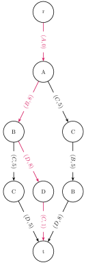
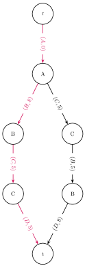
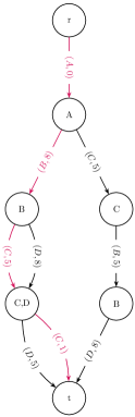
Exact Diagram	Restricted Diagram	Relaxed Diagram
$z^{*}={[A,B,D,C]}$	$z^{*}={[A,B,C,D]}$	$z^{*}={[A,B,C,C]}$
$T^{*}=17$	$T^{*}=18$	$T^{*}=14$

Figure 2: MDD Representation for the SOP instance presented in Figure 1. Each arc $a$ has the format: $(l,v(a))$. The red path in each diagram indicates the shortest path from $r$ to $t$.

Figure 1 gives an instance of sequence ordering problem (SOP), and Figure 2 contains simple examples of exact, restricted, and relaxed decision diagrams for that instance where $w_{m}=2$ for $\overline{\mathcal{M}}$ and $\underline{\mathcal{M}}$.

The SOP requires finding the minimum-cost sequence of $n$ elements that includes each element exactly once, subject to transition costs $c_{ij}$ of following $x_{i}$ with $x_{j}$, and subject to precedence constraints requiring that certain elements precede others in the sequence. In other words, the SOP is an asymmetric TSP with precedence constraints. The label of each node matches the union of the labels of the incoming arcs. Each arc $a_{uv}$ is labeled in the format $(l,val(a_{uv}))$, representing the assignment of $x_{\ell_{u}}$ to $l$, and $val(a)$ represents the cost of the shortest path from the label of $u$ to $l$. In other words, an arc with label $l$ leaving layer $i$, represents the assignment of $l$ to the $i^{th}$ position of the sequence. The red path in each diagram indicates the shortest path through the diagram, and $T^{*}$ indicates the cost of the shortest path through the diagram.

2.2 Restricted Decision Diagrams

Constructing $\overline{\mathcal{M}}$ for a given width $w_{m}$ is a straightforward process that can be thought of as a generalized greedy algorithm. Beginning with the root node $r$, an arc is generated for every element in the domain of $r$, and a node is generated at the end of each arc in the second layer. The process is repeated for each layer, except layer $n$ where all outgoing arcs point to the terminal, unless $w(\overline{\mathcal{M}})$ exceeds $w_{m}$. Then the least promising node is removed from the offending layer until $w(\overline{\mathcal{M}})$ is equal to $w_{m}$. The definition of least promising is a heuristic decision. For the purposes of this paper, the least promising node is the node $u$ such that the shortest path from $r$ to $u$ is longer than the shortest path from $r$ to any other node $v\neq u$ in layer $\ell_{u}$. In other words, nodes with the worst associated partial solutions are chosen for removal.

It is of note that another method of reducing the width of $\overline{\mathcal{M}}$ is merging equivalent nodes. In the SOP, two nodes can be considered equivalent if they have the same state (last element in the sequence), and all incoming paths have visited the same set of elements. For example, a node with exactly one incoming path $[A,B,C]$ could be merged with a node in the same layer with exactly one incoming path $[B,A,C]$. In many MDD applications this is a valuable insight, and it helps motivate the algorithm for constructing $\underline{\mathcal{M}}$. However, for the SOP, we observed that the work of finding equivalent nodes in $\overline{\mathcal{M}}$ often outweighed the benefit of being able to merge nodes, and our implementation of restricted decision diagrams does not currently leverage equivalent node merging.

2.3 Relaxed Decision Diagrams

There are many methods of constructing relaxed decision diagrams, and many heuristic decisions that must be made when doing so. In this paper, we focus on the method described by Cire & van Hoeve (2013) for sequencing problems. As opposed to the top-down construction described in Section 2.2, here $\underline{\mathcal{M}}$ will be constructed by separation. Constructing DDs by separation uses $\underline{\mathcal{M}}$ as a domain store over which constraints can be propagated. This method starts with a weak relaxation, and then strengthens it by splitting nodes until each layer is either exact, or has a width equal to $w_{m}$. The algorithm begins from a $1$-width MDD with an arc from the node on layer $\ell_{i}$ to the node on layer $\ell_{i+1}$ for each element that can be placed at position $\ell_{i}$ in the sequence. Thus, even though each layer only has one node, there can be several arcs between layers (see the relaxed diagram in Figure 2). Then a node $u$ is selected and split to strengthen the relaxation. The process of splitting $u$ involves creating two new nodes $u^{\prime}_{1}$ and $u^{\prime}_{2}$, and then distributing the in arcs of $u$ between $u^{\prime}_{1}$ and $u^{\prime}_{2}$. Then for each out arc $a_{uv}$ from $u$, arcs $a_{u^{\prime}_{1}v}$ and $a_{u^{\prime}_{2}v}$ are added such that $a_{uv}$, $a_{u^{\prime}_{1}v}$ and $a_{u^{\prime}_{2}v}$ all have the same label. Finally $u^{\prime}_{1}$ and $u^{\prime}_{2}$ are filtered to remove infeasible and sub-optimal arcs. A collection of filtering rules are used to check each arc. As an example, given a feasible solution to $\mathcal{P}$ with objective value $z_{opt}$, an arc $a$ can be removed if all paths containing $a$ have an objective value greater than $z_{opt}$. The full process of identifying which arcs can be removed is detailed in (?), and is not replicated here.

The following notation and definitions are critical to understanding these algorithms. Let $All_{u}^{\downarrow}$ be the set of arc labels that appear in every path from $r$ to $u$. Let $Some_{u}^{\downarrow}$ be the set of arc labels that appear in at least one path from $r$ to $u$. Let $All_{u}^{\uparrow}$ and $Some_{u}^{\uparrow}$ be defined as above, except that they refer to paths from $u$ to $t$. Let $\mathscr{J}$ be the set of all possible arc labels. For the SOP, we define an exact node $u$ as a node where $Some_{u}^{\downarrow}=All_{u}^{\downarrow}$ and all arcs ending at $u$ originate from exact nodes. Intuitively, a node $u$ is exact if all paths to $u$ contain the same set of labels, and all parents of $u$ are exact. The $All$ and $Some$ notation was originally introduced by introduced by Andersen et al. (2007). Algorithm 1 formalizes the process of strengthening $\underline{\mathcal{M}}$.

1 Let $\underline{\mathcal{M}}$ be an MDD such that $Sol(\underline{\mathcal{M}})\supseteq Sol(\mathcal{P})$

2 for layer $L_{j}\in\underline{\mathcal{M}}$ from $j=1$ to $j=n$ do

3       while $|L_{j}|<w_{m}$ and $\exists$ some node $y\in L_{j}$ such that $y$ is not exact do

4             $\mathscr{J}\leftarrow$ getAssignmentOrdering($\mathcal{P}$)

5             The getAssignmentOrdering() function returns a heuristically defined ordering of the values that can be assigned to decision variables

6             for $\phi\in\mathscr{J}$ while $|L_{j}|<w_{m}$ do

7                   $S\leftarrow$ selectNodes($L_{j}$,$\phi$)

8                   The selectNodes() function returns the set of nodes $u\in L_{j}$ such that $\phi\in Some_{u}^{\downarrow}\backslash All_{u}^{\downarrow}$

9                   for $u\in S$ while $|L_{j}|<w_{m}$ do

10                         Create two new nodes $u_{1}^{\prime},u_{2}^{\prime}$

11                         $L_{j}\leftarrow(L_{j}\cup\{u_{1}^{\prime},u_{2}^{\prime}\})$

12                         foreach arc $a_{vu}$ do

13                               if $\phi\in(All_{v}^{\downarrow}~{}\cup$ the label of $a)$ then

14                                    Redirect $a$ such that $a_{vu_{1}^{\prime}}$

15                              else

16                                    Redirect $a$ such that $a_{vu_{2}^{\prime}}$

17                               end if

18                              

19                         end foreach

20                        foreach arc $a_{uv}$ do

21                               Create arcs $a_{u_{1}^{\prime}v}$ and $a_{u_{2}^{\prime}v}$ such that $label(a_{uv})=label(a_{u_{1}^{\prime}v})=label(a_{u_{2}^{\prime}v})$

22                               filter($a_{u_{1}^{\prime}v}$), filter($a_{u_{2}^{\prime}v}$)

23                               filter($a$) runs a list of quick checks to see if an arc can be removed

24                              

25                         end foreach

26                        $L_{j}\leftarrow(L_{j}\backslash u)$

27                        

28                   end for

29                  

30             end for

31            

32       end while

33      

34 end for

return $\underline{\mathcal{M}}$

Algorithm 1 Refining Decision Diagrams for Sequencing (?)

Deciding which nodes to split, and how to split them, are heuristic decisions with a significant impact on the bound that can be achieved without exceeding $w_{m}$ (?). The algorithm discussed here selects nodes that can be split into equivalency classes, such that every path to the new node contains a certain label. Deciding which equivalency classes to produce first is another heuristic decision. The details of ordering the importance of the labels are specific to the problem being solved, and are not discussed here. However, it is important to note that the ordering for this implementation is static, and does not change between iterations.

2.4 Branch-and-Bound with Decision Diagrams

In a typical branch-and-bound algorithm, the branching takes place by splitting on the domain of the variables. With decision diagrams, the branching takes place on the nodes themselves by selecting a set of exact nodes to represent the problem. The solver outlined by Bergman et al. (2016b) defines an exact node as a node $u$ for which every path from $r$ to $u$ ends in an equivalent state. As mentioned above, we can be more specific when applying this to sequencing problems, and define an exact node $u$ as a node where $Some_{u}^{\downarrow}=All_{u}^{\downarrow}$ and all arcs ending at $u$ originate from exact nodes. An exact cutset is defined as a set of exact nodes that contain every path from $r$ to $t$. Let $\underline{\mathcal{M}}(u)$ be a relaxed decision diagram with root $u$, and let $\overline{\mathcal{M}}(u)$ be a restricted decision diagram with root $u$. The branch-and-bound algorithm for MDDs proceeds by selecting an exact cutset of $\underline{\mathcal{M}}$, and using each node $u$ in the cutset as the root for a new restricted decision diagram $\overline{\mathcal{M}}(u)$ and relaxed decision diagram $\underline{\mathcal{M}}(u)$. A node can be removed from the queue if the relaxation of that node is not better than the best known solution to $\mathcal{P}$, otherwise the exact cutset of the new node is added to the queue, and the process repeats until the queue is empty. This is detailed by Algorithm 2.

Gillard et al. 2021) expanded on Algorithm 2 by incorporating a local search. A heuristic is used to quickly calculate a rough relaxed bound at each node, and if the length of the shortest path to that node plus the rough relaxed bound is worse than the best known solution, the node can be removed. More formally, let $rrb(u)$ be a rough relaxed bound on $\mathcal{P}$ starting from node $u$, and let $z_{opt}$ be the value of best known solution so far. If $T^{*}(u)+rrb(u)>z_{opt}$, the node can be removed. They also provide evidence that if $rrb(u)$ is inexpensive to compute, it can be used to filter nodes in $\overline{\mathcal{M}}$ and $\underline{\mathcal{M}}$. The method of using a rough relaxed bound to trim nodes is used in this paper, but the details are problem specific and are discussed in a later section.

1 Let $\underline{\mathcal{M}_{uu^{\prime}}}$ be a partial diagram with root $u$ and terminal $u^{\prime}$

2 Let $v^{*}(u)$ be the lower bound of $\mathcal{P}$ resulting from starting at node $u$

3 Let $z_{opt}$ be the value of the best known solution

4 $Q=\{r\}$

5 $v^{*}(r)\leftarrow 0$

6 $z_{opt}\leftarrow\infty$

7 while $Q\neq\emptyset$ do

8       $u\leftarrow$selectNode($Q$), $Q\leftarrow Q\backslash\{u\}$

9       $\overline{\mathcal{M}}\leftarrow\overline{\mathcal{M}}(u)$

10       if $v^{*}(\overline{\mathcal{M}})<z_{opt}$ then

11            $z_{opt}\leftarrow v^{*}(\overline{\mathcal{M}})$

12       end if

13      if $\overline{\mathcal{M}}$ is not exact then

14             $\underline{\mathcal{M}}\leftarrow\underline{\mathcal{M}}(u)$

15             if $v^{*}(\underline{\mathcal{M}})<z_{opt}$ then

16                   $S\leftarrow$ exactCutset($\underline{\mathcal{M}}$)

17                   foreach $u^{\prime}\in S$ do

18                         let $v^{*}(u^{\prime})=v^{*}(u)+v^{*}(\underline{\mathcal{M}_{uu^{\prime}}})$

19                         $Q\leftarrow Q\cup u^{\prime}$

20                        

21                   end foreach

22                  

23             end if

24            

25       end if

26      

27 end while

return $z_{opt}$

Algorithm 2 Decision Diagram based Branch-and-Bound (BnB) (?)

3 Peel-and-Bound Algorithm

The motivation for peel-and-bound stems from an observation about Algorithm 1. When implemented in a branch-and-bound structure, a large portion of the work done while generating each $\underline{\mathcal{M}}$ is repeated at every iteration. Creating the relaxation for some exact node $u$ in the queue requires creating a $1$-width decision diagram, iterating over each layer from the top down, and splitting nodes in a predetermined order. The static order of node splits means that for each node $y$ such that $\ell_{y}>\ell_{u}$, the first equivalency class created when splitting $y$ is the same in $\underline{\mathcal{M}}(r)$ and $\underline{\mathcal{M}}(u)$. The existing arcs for both diagrams will be sorted in the same way, and the only difference is the possibility of filtering arcs in $\underline{\mathcal{M}}(u)$ that could not be filtered in $\underline{\mathcal{M}}(r)$ due to the added constraint that all paths must pass through $u$. The extra filtered arcs are the reason that $\underline{\mathcal{M}}(u)$ may produce a stronger bound than $\underline{\mathcal{M}}(r)$. However, because equivalency classes are chosen in the same order each time, many arcs that were filtered while constructing $\underline{\mathcal{M}}(r)$ will also be filtered again while constructing $\underline{\mathcal{M}}(u)$. There is a sub-graph of $\underline{\mathcal{M}}(r)$, induced by node $u$, that contains all of the paths that will be encoded in $\underline{\mathcal{M}}(u)$, but does not contain the arcs that are filtered from both diagrams during construction. Thus, less work needs to be performed at each iteration of branch-and-bound by starting from that sub-graph instead of a $1$-width diagram. If the split order is static, the same diagram is generated starting from either the $1$-width diagram, or the sub-graph induced by $u$. If the split order changes between branch-and-bound iterations, the sub-graph induced by $u$ is still a valid relaxation, but the generated diagram will differ from one that began at width $1$.

Consider a SOP instance where the goal is to order the elements $[A,B,C,D]$, subject to the precedence constraint that $A$ must precede $D$, an alphabetical ordering heuristic, and $w_{m}=3$. Figure 3 shows $\underline{\mathcal{M}}(r)$, and $\underline{\mathcal{M}}(A)$ in three stages. The first stage is the initial $1$-width diagram. The second stage is after one split on each layer, and the third stage is the complete diagram. The sub-graph shared by $\underline{\mathcal{M}}(r)$ and $\underline{\mathcal{M}}(A)$ is highlighted in blue, indicating that in this case the first two splits could have been read from $\underline{\mathcal{M}}(r)$ instead of being re-created from scratch.

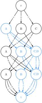
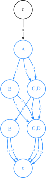
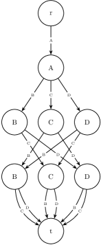
$\underline{\mathcal{M}}(r)$	$\underline{\mathcal{M}}(A)$ Stage 1	$\underline{\mathcal{M}}(A)$ Stage 2	$\underline{\mathcal{M}}(A)$ Stage 3

Figure 3: Example of a sub-graph (shown in blue), and the associated relaxed decision diagram with the same root for a SOP instance. The objective is to order the elements $[A,B,C,D]$, subject to the precedence constraint that $A$ must precede $D$, an alphabetical ordering heuristic, and $w_{m}=3$.

This mechanism can be embedded into a slightly modified version of the standard branch-and-bound algorithm based on decision diagrams (Algorithm 2). In peel-and-bound, the queue stores diagrams instead of nodes. After the initial relaxation $\underline{\mathcal{M}}(r)$ is generated, the entire diagram is placed into the queue $Q$ such that $Q=\{\underline{\mathcal{M}}(r)\}$. Then a diagram $\underline{\mathcal{M}}(u)$ is selected from $Q$ (for the first iteration $\underline{\mathcal{M}}(u)=\underline{\mathcal{M}}(r)$). However, instead of selecting an exact cutset of $\underline{\mathcal{M}}(u)$, a single exact node $e$ from $\underline{\mathcal{M}}(u)$ is selected. The process of selecting a diagram and exact node are heuristic decisions that are discussed in Section 3.2. The process of peeling $e$ is as follows. Create an empty diagram $\underline{u}$, remove $e$ from $\underline{\mathcal{M}}(u)$, and then put $e$ into $\underline{u}$ such that $e$ is the root of $\underline{u}$, and the arcs leaving $e$ still end in $\underline{\mathcal{M}}(u)$. Then for each node $y$ in $\underline{\mathcal{M}}(u)$ with an in arc that originates in $\underline{u}$, a new node $y^{\prime}$ is made and added to $\underline{u}$. Each in arc $a_{oy}$ of $y$ that originates in $\underline{u}$ is removed and then arc $a_{oy^{\prime}}$ is added to $\underline{u}$. Then the out arcs of $y$ and $y^{\prime}$ are filtered using the same filter function as Algorithm 1. The process of removing and adding arcs is repeated until there are no arcs ending in $\underline{\mathcal{M}}(u)$ that originate in $\underline{u}$. This procedure accomplishes a top-down reading of the sub-graph induced by $e$, and potentially strengthens $\underline{\mathcal{M}}(u)$ by removing nodes and arcs in the process. If the shortest path through the modified $\underline{\mathcal{M}}(u)$ is less than the best known solution, $\underline{\mathcal{M}}(u)$ is put back into $Q$. The diagram $\underline{u}$ is relaxed using Algorithm 1. Let $\underline{\mathcal{M}}(\underline{u})$ be the result; then if the shortest path through the refined diagram $\underline{\mathcal{M}}(\underline{u})$ is less than the best known solution, $\underline{\mathcal{M}}(\underline{u})$ is added to $Q$. The whole procedure is repeated until there are no nodes left in the queue ($Q=\emptyset$). A peel operation is illustrated and explained in Figure 4. Peel-and-bound is formalized in Algorithm 3, and the peel operation is formalized in Algorithm 4.

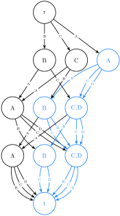
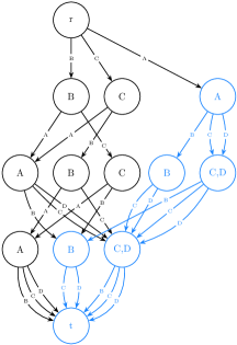
(1)	(2)
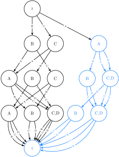
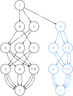
(3)	(4)

Figure 4: An example of a peel operation. In (1), $A$ is selected to induce the peel process and removed from the the original diagram ($\underline{\mathcal{M}}(r)$ from Figure 3). In (2) the arcs that connect $A$ to the original diagram are moved to copies of the nodes they originally ended at, and infeasible arcs are filtered. In (3) and (4) the process is repeated until the diagrams are disconnected.

1 Let $v^{*}(u)$ be the lower bound of $\mathcal{P}$ resulting from starting at node $u$

2 Let $z_{opt}$ be the value of the best known solution

3 $Q=\{\underline{\mathcal{M}}(r)\}$

4 $z_{opt}\leftarrow\infty$

5 while $Q\neq\emptyset$ do

6       $\mathscr{D}\leftarrow$selectDiagram($Q$), $Q\leftarrow Q\backslash\{\mathscr{D}\}$

7       $u\leftarrow$selectExactNode($\mathscr{D}$)

8       $\underline{u},\mathscr{D}^{*}\leftarrow$ peel($\mathscr{D}$, $u$) (See Algorithm 4)

9       if $v^{*}(\mathscr{D}^{*})<z_{opt}$ then

10             $Q\leftarrow Q\cup\{\mathscr{D}^{*}\}$

11       end if

12      $\overline{\mathcal{M}}\leftarrow\overline{\mathcal{M}}(u)$

13       if $v^{*}(\overline{\mathcal{M}})<z_{opt}$ then

14            $z_{opt}\leftarrow v^{*}(\overline{\mathcal{M}})$

15       end if

16      if $\overline{\mathcal{M}}$ is not exact then

17             $\underline{\mathcal{M}}\leftarrow\underline{\mathcal{M}}(\underline{u})$

18             if $v^{*}(\underline{\mathcal{M}})<z_{opt}$ then

19                   $Q\leftarrow Q\cup\{\underline{\mathcal{M}}\}$

20             end if

21            

22       end if

23      

24 end while

return $z_{opt}$

Algorithm 3 Peel-and-Bound (PnB) Algorithm

1 Let $in(u)$ for some node $u$ be the set of arcs that end at node $u$

2 Let $out(u)$ for some node $u$ be the set of arcs that originate from node $u$

3 Let $in(\mathcal{M})$ for some MDD $\mathcal{M}$ be the set of arcs that end in $\mathcal{M}$

4 Let $out(\mathcal{M})$ for some MDD $\mathcal{M}$ be the set of arcs that originate in $\mathcal{M}$

5 input: a relaxed MDD $\mathscr{D}$, and an exact node $u$ in $\mathscr{D}$

6 output: a relaxed MDD $\underline{u}$ peeled from $\mathscr{D}$, and what remains of relaxed MDD $\mathscr{D}$

7 Let $\underline{u}$ be an empty decision diagram

8 $in(u)\leftarrow\emptyset$

9 $\mathscr{D}\leftarrow\mathscr{D}\backslash u$

10 $\underline{u}\leftarrow u$

11 while $in(\mathscr{D})\cap out(\underline{u})\neq\emptyset$ do

12       foreach node $m\in\mathscr{D}$ with an in arc that originates in $\underline{u}$ do

13             create a new node $m^{\prime}$, and add it to $\underline{u}$

14             foreach arc $a\in in(m)$ that originates in $\underline{u}$ do

15                   change the destination of $a$ to $m^{\prime}$

16                   filter($a$)

17             end foreach

18            foreach arc $a\in out(m)$ do

19                   filter($a$)

20             end foreach

21            

22       end foreach

23      

24 end while

25while $\exists$ some node $m\in D$ with $in(m)=\emptyset$ or $out(m)=\emptyset$ (excluding $r$ and $t$) do

26       $in(m)\leftarrow\emptyset$

27       $out(m)\leftarrow\emptyset$

28       $\mathscr{D}\leftarrow\mathscr{D}\backslash\{m\}$

29 end while

return ($\underline{u}$, $\mathscr{D}$)

Algorithm 4 Peeling process used in Algorithm 3

3.1 Complexity Analysis

Separating each node $u$ during a peel requires creating a new node $u^{\prime}$, moving the in arcs of $u$ that originate in the peeled diagram $\underline{u}$ to $u^{\prime}$, copying the out arcs of $u$ to $u^{\prime}$, and then filtering the out arcs of $u$ and $u^{\prime}$. Creating a new node in our implementation has a time in $\mathcal{O}(n)$, where $n$ is the number of elements in the sequence (or the number of possible decisions in a more generic problem), due to storing state information that has a size in $\mathcal{O}(n)$ (such as $All_{u^{\prime}}^{\downarrow}$). However, it is possible that in other applications the size of a node is in $\mathcal{O}(1)$. The number of in arcs of $u$ is at most $w$, although this worst case is unlikely in practice because it requires $\underline{u}$ to have width $w$ and for each node in $\underline{u}$ on layer $\ell_{u}-1$ to have an arc ending at $u$. Thus, moving the in arcs of $u$ has a time in $\mathcal{O}(w)$. The number of out arcs of $u$ is at most $n$, and each arc has a size in $\mathcal{O}(1)$, so copying the out arcs has a time in $\mathcal{O}(n)$. Each individual filtering process has a time in $\mathcal{O}(1)$ as it uses only existing state information from $u$ and $u^{\prime}$, and it is performed on the at most $2n$ out arcs of $u$ and $u^{\prime}$. Thus, filtering the out arcs has a time in $\mathcal{O}(n)$. Therefore, separating one node during the peel process has a time in $\mathcal{O}(n+w)$. Separations during a standard relaxation procedure require selecting a node ($\mathcal{O}(w)$), making a new node ($\mathcal{O}(n)$), partitioning the in arcs ($\mathcal{O}(nw)$), copying the out arcs ($\mathcal{O}(n)$), and filtering the out arcs ($\mathcal{O}(n)$). The reason that there can be more in arcs during a standard relaxation procedure is because the nodes in a $1$-width diagram can have in arcs with different labels coming from the same node, whereas the structure of the diagram during a peel guarantees that each node $u$ can have only one in arc from each node on the layer $\ell_{u}-1$. Thus, the total time for a separation in a standard relaxation is in $\mathcal{O}(nw)$.

The maximum number of separations during a peel is the maximum number of nodes in the peeled diagram. A peeled diagram can have at most $(n-3)\times w+2$ nodes, and thus the number of nodes is in $\mathcal{O}(nw)$. Therefore, the entire peel process has a time in $\mathcal{O}(n^{2}w+nw^{2})$. The maximum number of separations during a standard relaxation is the exact same as during a peel, since the resulting diagram will be the same size. Thus, the standard relaxation has a total time in $\mathcal{O}(n^{2}w^{2})$. However, peel-and-bound uses a peel to generate some fraction of the nodes, then a standard relaxation to generate the rest. Let $\alpha$ be the percent of nodes that are peeled during the peel. It follows that the total time for an iteration of peel-and-bound is in $\mathcal{O}(\alpha(n^{2}w+nw^{2})+(1-\alpha)(n^{2}w^{2}))$. Therefore, the larger that $\alpha$ grows, the more time peel-and-bound saves over branch-and-bound.

3.2 Advantages and Implementation Decisions

3.2.1 Node Selection

The branch-and-bound algorithm proposed by Bergman et al. (2016b) requires selecting an exact cutset of $\underline{\mathcal{M}}$. Peel-and-bound requires selecting a diagram from the queue, and an exact node to start the peel process. The choice of node has a substantial impact on how quickly the process converges to an optimal solution, because it serves two purposes simultaneously. As discussed earlier, the first purpose of peeling is to avoid recreating a portion of the diagram at each iteration. The second purpose is to strengthen the overall relaxation. Let $\underline{u}$ be a diagram peeled from $\underline{\mathcal{M}}$, and let $\underline{\mathcal{M}}^{*}$ be $\underline{\mathcal{M}}$ after the peel operation. If $Sol(\mathcal{P})\subseteq Sol(\underline{\mathcal{M}})$ then $Sol(\mathcal{P})\subseteq Sol(\underline{\mathcal{M}}^{*})\cup Sol(\underline{u})$. The only step of peel-and-bound that removes paths is the filter step, which only removes an arc if no feasible solutions can pass through that arc. If the node the peel is induced from contains the shortest path through $\underline{\mathcal{M}}$, then there will be a new shortest path through $\underline{\mathcal{M}}^{*}$ with $T^{*}(\underline{\mathcal{M}}^{*})\geq T^{*}(\underline{\mathcal{M}})$. Similarly after peeling, the peeled diagram is going to be strengthened and $T^{*}(\mathcal{M}(\underline{u}))\geq T^{*}(\underline{u})$. Therefore, when implementing the selectDiagram and selectExactNode functions from Algorithm 3, we propose selecting the diagram $\mathscr{D}$ containing the most relaxed bound, and an exact node from $\mathscr{D}$ that contains $z^{*}(\mathscr{D})$ at each iteration. Using these parameters, the peel step of peel-and-bound strengthens the relaxed bound of $\mathcal{P}$, in addition to providing a stronger initial diagram to use when generating $\mathcal{M}(\underline{u})$.

We originally proposed two heuristics for selecting a node from $\mathscr{D}$ that contains $z^{*}(\mathscr{D})$. The first heuristic picks the first node in the shortest path through the diagram with at least one child that is not exact, we call this the last exact node. The second heuristic picks the frontier node, the highest-index exact node that contains $z^{*}(\mathscr{D})$. Taking the last exact node is more of a breadth-first search that peels a large set of nodes where all of the paths to the nodes in the set share a beginning with $z^{*}(\mathscr{D})$. In contrast, taking the frontier node is more of a depth-first search, taking fewer nodes and exploring those nodes at greater depth. We have since experimented with a third heuristic where we pick what we call the maximal node. The maximal node is simply the node on the second layer that contains $z^{*}(\mathscr{D})$. This peels as many nodes as possible while still picking a node that contains $z^{*}(\mathscr{D})$.

3.2.2 Handling Non-Separable Objective Function

When a problem is represented with an Integer Program, the value or cost of making a decision is separate for each variable; in other words the objective function is separable. However, when using MDDs to represent a problem, the objective function can be non-separable. In the example SOP used in Section 2, the cost of an arc leaving a node $u$ is dependent on the labels of the arcs that end at $u$. If the arcs have conflicting labels, then arcs leaving $u$ may not have an exact cost. Cire & van Hoeve (2013) proposed that each iteration of Algorithm 1 starts from a $1$-width MDD. However, for peel-and-bound with a non-separable objective function, starting from a $1$-width MDD poses a problem. The arcs in such a diagram do not have exact values, because they are dependent on the state of the node they originate from. As nodes are peeled, the values of those arcs must be updated, and the operation becomes computationally expensive at scale.

When solving sequencing problems where the non-separability of transition costs arises from their dependency on the previous element in the sequence, this problem can be avoided by creating the initial diagram using a structure where all of the arcs ending at a given node have the same label. The resulting initial diagram has a width of $n$, and each node on the layer is assigned to one state $s\in\{1,...,n\}$. Then every possible feasible arc between consecutive layers is added. Thus, the nodes of $\underline{\mathcal{M}}$ do not have relaxed states, and each arc can only take one possible value. Starting from such a diagram not only removes the need to update arc values, it ensures that every arc generated during peel-and-bound is an exact copy of an arc that exists in the initial diagram, since arcs are only copied or removed, never updated or added. Using this structure makes implementation easier by removing the need to store any information on the arcs at all. As each node will only have one state $s$, the label and weight of an arc is implied by the state of the node it originates from, and the node it points to. This allows all information in a diagram to be stored on the nodes, and thus only the information on the nodes ever needs to be read or updated.

When transition costs are dependent on factors other than the previous element in a sequence, such as the Time-Dependent TSP (TSP-TD), modifications to the described method become necessary. In general an exact cost may not be calculable, but a relaxed bound on cost can be made calculable by storing the relevant values as a range at each node. Consider an MDD for the TSP-TD where nodes $u$ and $v$ are connected by an arc. Let $a_{u}$ to $b_{u}$ be the range of possible times one can arrive at $u$. While an exact cost for the arc from $u$ to $v$ is not available, a relaxed bound can be found by varying the time from $a_{u}$ to $b_{u}$, and then using the best value found as the cost. As the MDD is peeled, the gap between $a_{u}$ and $b_{u}$ may grow smaller, but it will never grow larger. When the gap decreases, the previously calculated cost is still a valid relaxed bound. Thus, the cost can be updated to retrieve an improved bound, but it is not necessary to do so with every peel operation. Many problems will require modifying this concept to fit their particular constraints, but this method is easy to adapt in most cases. An alternative method of handling non-separable objective functions is explored by (?, ?, ?).

3.2.3 Parallelization

The decision diagram based branch-and-bound shown in Algorithm 2 is particularly amenable to parallelization as shown by Bergman et al. (2014b) and again by Gillard (2022). Algorithms seeking to parallelize must overcome the data-race problem. In other words, if multiple processors are working on a problem simultaneously, then there must be a process in place to stop them from trying to write to the same place in memory at the same time. For many algorithms, this poses a substantial challenge or creates substantial overhead. However, for both decision diagram based branch-and-bound, and peel-and-bound, the solution is simple. As a problem is being solved, nodes (or diagrams in the case of peel-and-bound) are placed into a processing queue. Each node/diagram represents a discrete problem that needs to be solved, and can be processed separately. Given access to a sufficiently large number of processors, each node/diagram added to the queue could be immediately dispatched to an available processor for processing. The only communication required between the processors is the current value of the best known solution. In theory, this could result in a linear improvement in time spent solving a problem when increasing the number of processors available, because $k$ processors may be able to process $k$ nodes, in the time it takes $1$ processor to process $1$ node. This process could also result in a superlinear speedup due to the non-deterministic processing order of elements in the queue. In the parallel implementation, one processor may find an improved bound which can then be utilized by the other processors. Therefore, elements from the queue could be processed using bounds that are better than the bounds used by the single-thread deterministic implementation. The ability to identify better bounds earlier on during parallel processing when processing an element could yield less elements that need to be processed overall. In practice, however, there are heuristic decisions that must be made that can have a large impact on solve time.

The dilemma one encounters in implementation is the existence of a critical path in the solution finding process. To demonstrate this with an extreme example, consider a problem that does the following when solved using peel-and-bound on a single processor. Each time a node is peeled, one of the two resulting diagrams is solved and closed without requiring any additional peel operations. Then the single remaining diagram is processed again, a node is peeled, and the whole process repeats itself $m$ times. In this example, there are roughly $2m$ diagrams that need to be processed, but only $2$ are ever available at the same time. So in this case, $k$ processors would take exactly as long as $2$ processors to solve the problem. We propose two methods of handling this dilemma. The first is simple; reduce the maximum width of the diagrams. When solving a problem that is encountering this critical path problem, the work can be divided more equitably among the available processors by reducing the amount of work done at each iteration. When using a single processor, a higher maximum width is almost always more desirable as long as the decision diagrams can still be generated quickly, because the extra space makes it more likely that the diagram will be solved instead of producing more diagrams to add to the queue. Reducing the maximum width will increase the number of diagrams that need to be processed to solve the problem, but also produces those diagrams more quickly. A width too low can generate an enormous number of diagrams without closing any of them. The optimal width to use is one that generates enough diagrams for all available processors to have consistent work, but does not generate a large backlog of work.

The second method of handling the critical path issue is to use the peel process to redistribute work as needed. Each time a processor is available and not being used, the peel procedure can peel off a sub-diagram for that processor to work on. The downside of this is that often a lot of the work that only needed to be performed once, will occur on both diagrams. The first method of simply lowering the maximim width accomplishes the same goal, but each diagram reaches its assigned maximum width before it is further processed, so arcs that can be processed out, only need to be processed out of one diagram. Any implementation of this second method would likely require more heuristic decisions to ensure the task scheduler distributes the work in a useful way.

3.2.4 Embedded Restricted Decision Diagrams

In both decision diagram based branch-and-bound (Algorithm 2), and peel-and-bound (Algorithm 3), at each branch a restricted decision diagram is created before the relaxed decision diagram. This is useful not just for solution finding, but also because the process of creating a restricted decision diagram is often several orders of magnitude faster than the process of refining a relaxed decision diagram. When the restricted decision diagram is exact, the relaxed decision diagram can be closed without any additional processing. Peel-and-bound provides an opportunity to leverage relaxed decision diagrams to improve the associated restricted decision diagrams.

The following idea extends the work done in Coppé et al. (2022). Each path from the root to a node in a restricted decision diagram represents a partial solution to the problem being solved. Any partial solution to the problem represents a partial path through a matching relaxed decision diagram. So each path to a node $\overline{u}$ in a restricted decision diagram $\overline{\mathcal{M}}$ can be mapped to exactly one node $\underline{u}$ in a relaxed decision diagram $\underline{\mathcal{M}}$. When generating $\overline{\mathcal{M}}$ from the top-down, each node in $\overline{\mathcal{M}}$ creates a child node on the next layer for every element in its domain (before the layer is trimmed down to the maximum width). We incorporate multiple methods from the literature for trimming this domain, such as the rough relaxed bound we will discuss in Section 3.4, but add our own here. Let $d(\overline{u})$ be the domain of $\overline{u}$; we set $d(\overline{u})=d(\overline{u})\cap d(\underline{u})$ before generating the child nodes of $\overline{u}$. There are two clear benefits to this strategy, that pair to the two reasons something can be in $d(\overline{u})$ but not $d(\underline{u})$. If an arc has been proven to be infeasible or sub-optimal, it will not be in $\underline{\mathcal{M}}$. However, the methods of that proof may not be available to nodes in $d(\overline{u})$. So our method prevents $\overline{M}$ from exploring nodes that have already been proven useless by $\underline{M}$. The other reason something can be in $d(\overline{u})$ but not $d(\underline{u})$ is that it was removed during a peel procedure performed on $d(\underline{M})$. Without using this intersection operation as a way to trim the domain, $\overline{\mathcal{M}}$ will search the entire solution space that starts from the same root as $\underline{\mathcal{M}}$, even if the peeled diagrams have already been closed as sub-optimal. Using this method, each restricted decision diagram will only search the solutions encoded within the matching relaxed decision diagram. This means that each restricted decision diagram has a significantly improved chance of closing the relaxed decision diagram it maps to, because the solution space it must explore becomes smaller with each peel.

3.2.5 Search Diversification

The structure of peel-and-bound yields another method of searching for solutions that forces increased diversification. The embedded restricted decision diagram described in Section 3.2.4 takes advantage of the reduced search space embedded in the relaxed decision diagram, but it makes no effort to explore substantially different regions, and thus it is at risk of getting stuck in a local optimum. Here we propose a simple method of diversifying the solutions explored. Starting from the root, and moving down layer by layer, map each node $u$ in the relaxed decision diagram to the best feasible path that ends at $u$, and is a continuation of a path a parent of $u$ maps to. The obvious drawback is that many paths will becomes infeasible or sub-optimal, and many of the relaxed nodes might not map to a feasible path using this method, simply because the paths that were being explored in their parents were bad paths. To fix this, the number of paths stored can be expanded. Let $k$ be any positive integer; if each node maps to the $k$ best paths to that node, then as the value of $k$ increases there is a much higher likelihood of new, and better, solutions being found. However, as the number of nodes in the diagram can be quite large, even small values of $k$ can be computationally expensive. So this method can be a powerful tool for diversification, but it comes with a significant drawback in terms of compute time. It has the potential to be valuable if used just once at the beginning of the peel-and-bound process to search for initial solutions, but is unlikely to be useful if repeated often. This idea may also benefit from being combined with the large neighborhood search using restricted decision diagrams proposed by Gillard & Schaus, (2022).

3.3 Limitations and Handling Memory

The focus of this paper is sequencing problems, but peel-and-bound can be easily applied to other optimization problems. However, some existing MDD based methods conflict with peel-and-bound. For example, some MDD algorithms use a dynamic variable order (?), such that the variables the layers on $\overline{M}$ are mapped to in one iteration of branch-and-bound, are different in the next. Peel-and-bound as it is presented in this paper cannot be paired with a dynamic variable order. Furthermore, the method in this paper is specific to decision diagrams generated using separation. We believe the method can be extended to decision diagrams that use a merge operator, but it has not been shown here.

Memory limitations present a problem for peel-and-bound in theory, but not in practice. Each open diagram remains in the queue, and thus must be stored in memory. However, this problem can be handled in many ways; two are given here. A dynamic method of handling the problem is to start targeting large diagrams with bounds close to $z_{opt}$ as memory limitations start to become a problem. Such diagrams can usually be closed quickly, and subsequently removed from memory, freeing up space for the algorithm to continue. Alternatively, the diagrams with bounds closest to $z_{opt}$ can be deleted in favor of storing just the root node, then when they need to be processed, initial diagrams are generated for those once again. This method essentially falls back to branch-and-bound until memory limitations cease to be a problem. Additional approaches for working with memory limitations, and evidence that the problem can be handled efficiently, are presented by Perez & Régin, (2018).

3.4 Integrating Rough Relaxed Bounds

This implementation incorporates the rough relaxed bounding method proposed by Gillard et al. (2021). Rough relaxed bounding was used to trim the domain of each node during construction of the restricted DDs, and was also added as a check to the filter function in Algorithm 1. When the initial model is created, a map is also created from each node $u$, to a list of the other nodes sorted by their distance from $u$. For the SOP, the rough relaxed bound $rrb(a)$ of an arc $a_{fg}$ was calculated as follows. For each node $u$ that has not necessarily been visited ($u\notin All_{g}^{\downarrow}$), look up the shortest distance from that node to a different node that has also not been visited. Then, sort the resulting list, and repeatedly remove the largest value until the list has a length equal to the number of remaining decisions. The sum of the values in the list, plus the value of the shortest path from $r$ to the end of $a$, is the rough relaxed bound of $a$. If $rrb(a)$ is worse than the best known solution, the arc is removed. Slight modifications were made to this procedure to extend it to the TSPTW and Makespan implementations used to generate the results shown in Section 5.

3.5 Peel-and-Bound with Top-Down Compilation

The structure of peel-and-bound is designed to take advantage of relaxed decision diagrams that are compiled by separation. Here we propose a method for applying peel-and-bound to relaxed decision diagrams that are compiled top-down. However, we have not tested this method, and it remains a topic of future research to determine if it would be useful in practice. The goal of peel-and-bound is to re-use work already done by reusing diagrams. When performing top-down compilation, nodes are merged instead of separated. The peel procedure can be used exactly as before, but after a node is peeled, the remaining diagrams must be altered so that new nodes can be added top-down using a merge procedure. However, there are no nodes to add, the diagrams already represent feasible bounds on the problem, and so some nodes must be removed. Begin by selecting a relaxed node $u$ (in other words some node $u$ that is not exact), and removing it from the diagram. Then remove any arcs in the diagram that are sub-optimal or no longer feasible due to the removed node. For each arc $a_{vu}$ that used to point to $u$, create a new arc $a_{vu\prime}$ that points to a new node $u\prime$ created by following the top-down compilation rules being used. Finally, proceed to perform top-down compilation using the set of new nodes as root nodes for the procedure.

4 Initial Experiments on the Sequence Ordering Problem

The goal of this section is to assess the performances of the peel-and-bound algorithm (PnB, Algorithm 3) as it compares to the standard decision diagram based branch-and-bound algorithm (BnB, Algorithm 2). Both algorithms are implemented in Julia and are open-source. To ensure a fair comparison, both algorithms resort to the same function for generating relaxed decision diagrams (Algorithm 1), and the same function for generating restricted decision diagrams. While the functions being called are the same, there are two differences at run-time. At the end of line $26$ in Algorithm 1, an additional operation runs during BnB where the values of the arcs leaving layer $j$ are updated. The second difference is that BnB starts each relaxation from a $1$-width DD, while PnB passes a partially completed diagram to the relaxation function as a starting point.

The testing environment was built from scratch to ensure a fair comparison, so it lacks the many propagators used by cutting-edge solvers like CPO to remove nodes from the PnB/BnB queue (?, ?). However, it provides a clean comparison of the two algorithms by requiring that every function used by both BnB and PnB is exactly the same between the two, with the only differences arising due to PnB’s ability to ensure that all arcs are exact from the beginning. All of the heuristic decisions that were made are identical for both algorithms. These experiments were performed before the implementation of maximal node selection (Section 3.2.1), unlabeled arcs (Section 3.2.2), embedded restricted decision diagrams (Section 3.2.4), and the search diversification procedure (Section 3.2.5), so those methods are not included in these experiments. An improved implementation that incorporates those methods and ideas is discussed in Section 5.

4.1 Description of the Heuristics Considered

The sequence ordering problem can be considered as an asymmetric travelling salesperson problem with precedence constraints. The objective is to find a minimum cost path that visits each of the $n$ elements exactly once, and respects the precedence constraints. The method used for generating relaxed DDs requires creating a heuristic ordering of all possible arc assignments by importance. The arc values in this case are representative of the $n$ elements in the path. The ordering used was generated by sorting the $n$ elements, first by their average distance from the other elements, and then by the number of elements each element must precede. The resulting order places a higher importance on elements that are far away from other elements and must precede many other elements.

The branch-and-bound algorithm processes nodes in an order designed to try and improve the existing relaxed bound at each iteration. When a node $u$ is added to the BnB queue, it is assigned a value equal to the value of the shortest path from the root $r$ to the terminal $t$, that passes through $u$. The best known relaxed bound on the problem is the smallest value of a node in the queue, and that node is always chosen to be processed. Peel-and-bound is implemented with the same goal of improving bounds at each iteration. However, PnB stores diagrams, not nodes. Let the value of a diagram be the value of the shortest path to the terminal. At each iteration of peel-and-bound, the diagram with the lowest value is selected, and then a node is chosen from that diagram to induce the peel process. All of the experiments here used a process where the selected node is the first node in the shortest path from $r$ to $t$ with a child node that is not exact (the last exact node). Testing was done to determine whether using the last exact node or the frontier node would perform better for the problem being considered, but there was not a significant difference between the two during any of the tests. Several of the benchmark problems were run using various decision diagram widths, and the last exact node was chosen because it sometimes showed a very slight improvement over the frontier node. While it is likely that this choice makes a difference on some problems, it does not matter for the SOP.

4.2 Experimental Results

The experiments were performed on a computer equipped with an AMD Rome 7532 at 2.40 GHz with 64Gb RAM. The solver was tested using DD widths of $64,128$, and $256$ on the $41$ SOP problems available in TSPLIB (?). For comparisons between PnB and BnB, a timestamp, new bounds, and the length of the remaining queue were recorded each time the bounds on a problem were improved. Another experiment was performed to test the scalability of PnB at width $2048$, for which only the final bounds were recorded. Execution time was limited to $3,600$ seconds.

The smallest DD width tested for both methods was $64$, and the largest DD width tested was $256$. Table 1 has summary statistics for those widths as the percentage improvement demonstrated by PnB. A positive percentage always indicates that PnB performed better than BnB in that category, while a negative percentage indicates that BnB performed better. Figure 5 shows performance profiles for all of the experiments. Table 2 contains summary statistics comparing PnB at width $256$ to PnB at width $2048$, where a positive percentage always indicates that the width of $2048$ performed better.

	Width: 64				Width: 256
	RB	BS	OG	QL	RB	BS	OG	QL
Average % Improvement	$114\%$	$0.5\%$	$22.8\%$	$1,647\%$	$545\%$	$3.3\%$	$181\%$	$308\%$
Median % Improvement	$26\%$	$0.05\%$	$17.4\%$	$734\%$	$80\%$	$1.7\%$	$35\%$	$141\%$

Table 1: Summary Statistics: percentage improvement of peel-and-bound over branch-and-bound. RB = Relaxed Bound, BS = Best Solution, OG = Optimality Gap, QL = Queue Length. Tables 5 and 6 in Appendix A show the comprehensive results.

	PnB: 2048 vs PnB: 256
	Relaxed Bound	Best Solution	Optimality Gap
Average % Improvement	$19.5\%$	$0.8\%$	$18.6\%$
Median % Improvement	$16.3\%$	$0.5\%$	$13.7\%$

Table 2: Summary Statistics: percentage improvement of peel-and-bound at width $2048$ over peel-and-bound at width $256$. Table 7 in Appendix A shows the comprehensive results.

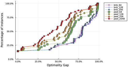
Figure 5: Performance Profiles: the optimality gap $=\frac{upper\_bound-lower\_bound}{upper\_bound}$

As shown in Table 1, peel-and-bound vastly outperforms branch-and-bound in these experiments. The average and median improvements from using peel-and-bound at both widths are significant in terms of the relaxed bound, the remaining optimality gap, and the number of nodes that still need to be processed. The best solution found by the end of the runtime also tends to be slightly better with peel-and-bound, but the found solutions are often so close to the real optimal solutions that there is little room for improvement. At both widths, six of the problems were solved to optimality. BnB was faster in only one of those cases, and in that case the difference was $.04$ seconds. The median time for PnB to close in these cases was $191\%$ faster at a width of 64, and $580\%$ faster at a width of $256$. The relaxed bound produced by PnB at a width of $64$ was better for $28$ of the remaining $35$ problems, and at a width of $256$ was better for $34$ of the remaining $35$ problems. The optimality gap was similarly better for peel-and-bound on every problem except the ones where branch-and-bound found a better relaxed bound. However, of the problems where branch-and-bound had a better optimality gap, the improvement was less than $1\%$ for all but one problem. Figure 5 reinforces that even though there are some instances where a specific branch-and-bound setting slightly outperforms a specific peel-and-bound setting, the gap in those cases is small relative to the general gap between all peel-and-bound settings and all branch-and-bound settings.

As shown in Table 2, increasing the width to $2048$ from $256$ led to an $19.5\%$ average improvement ($16.3\%$ median improvement) in the relaxed bound. Figure 5 shows that the performance of peel-and-bound nearly uniformly increases with the maximum allowable width. Similar to the difference between branch-and-bound and peel-and-bound, some specific instances see a small out-performance of the peel-and-bound running at a smaller width, but the gap is small relative to the usual gap between the $2048$-width experiment and the rest of the experiments. Additionally, Figure 5 shows that peel$\_2048$ solved $50\%$ of instances to within a $42\%$ optimality gap, peel$\_64$ solved $50\%$ of instances to within a $67\%$ optimality gap, and the best performing branch and bound (bnb$\_64$) solved $50\%$ of instances to within only a $79\%$ optimality gap. The overall performance of peel-and-bound improves as more problems are considered, especially as the maximum allowable width for the decision diagrams is increased.

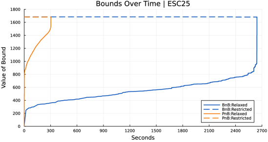
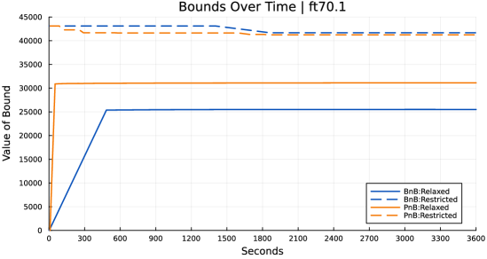
Figure 6: Dual bounds over the runtime of the experiment for ESC25, which was solved within the time limit, and ft70.1, which was not solved within the time limit. Both use a width of 256.

The selected graphs shown in Figure 6 are representative of the two main types of behavior observed over the problem set. On problems where the underlying relaxation method works well, the relaxed bound moves quickly towards convergence with the best found solution. On problems where the underlying relaxation does not work well, both algorithms slowly improve the relaxed bound, but PnB starts stronger as it can use exact arc values, and it maintains the advantage throughout. It is clear from the time-series data that to be competitive with cutting-edge solvers, peel-and-bound must be combined with other constraint programming propagators. However, it is also clear that peel-and-bound can have a significant edge over a propagator that generates the required decision diagrams from scratch at each iteration.

5 Experiments with Improved Methods

The first implementation of peel-and-bound, which was used to generate the results in Section 4, was designed to create a fair comparison of peel-and-bound and branch-and-bound; it was also limited to the SOP. We have since re-implemented peel-and-bound so the implementation is generic. The new version is similarly open-source, and all of the data from the following experiments can be found with the code. In this section, we further explore the performance of the algorithm and compare the performance of a subset of the heuristic methods proposed in Section 3. The experiments were performed on a computer equipped with an AMD Rome 7532 at 2.40 GHz with 186Gb RAM.

5.1 Node Selection Heuristic

In Section 3.2.1, we propose three heuristics for selecting a node to be peeled: frontier, last exact node, and maximal. Here we compare the performance of those three different settings on the same set of SOP instances we tested in Section 4; we similarly limit the runtime of the solver to 3600 seconds. We include the results from the most successful run performed by the original implementation of peel-and-bound to show how much the new implementation has improved in general. The results are shown in Figure 7. The first graph is a scatter-plot displaying the solve time of each problem that was solved to optimality, for each of the three node selection settings. The second graph shows performance profiles for the same tests, and includes data from the best run of the first implementation of peel-and-bound to show the overall improvement of the solver. All of the new tests were performed using 2048 as the maximum width, and included a diversified search with $k=5$ using the procedure described in Section 3.2.5.

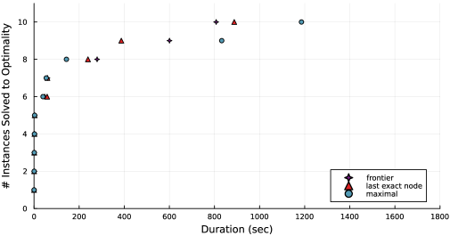
SOP Instances Solved over Time: max width of 2048

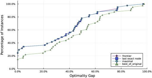
Performance Profiles on the SOP: max width of 2048

Figure 7: Performance of Peel-and-Bound on SOP.

Figure 7 makes it clear that choosing between the node selection heuristics has little effect on solving the SOP. The number of instances solved to optimality is identical, with the maximal having a slight lag on the final two problems, and the performance profiles are nearly identical. The performance profiles also serve to demonstrate the progress of the solver, with the percentage of instances closed to any given optimality gap being about 10% higher.

5.2 Traveling Salesman Problem with Time Windows

The traveling salesman problem with time windows (TSPTW) is a variation of the traveling salesman problem where a salesman must find the shortest cycle that visits each of his customers once, but each customer may have an added constraint requiring they be visited within a specific time window. It provides a useful metric for benchmarking the performance of the implementation of peel-and-bound, as decision diagram focused algorithms are more likely to outperform traditional methods on highly constrained problems than highly unconstrained problems, and the TSPTW instances are highly constrained. For the following tests we include both a standard and seeded run of the solver, where seeded means that the solver started out knowing the value of the best known solution, and skipped the initial diversified search. The seeded version is of interest because the solver can leverage heuristically generated solutions to reach proof of optimally faster. The difference between the standard and seeded run help may help to determine if taking that step is worthwhile when solving a specific problem. We test our solver on the same set of $467$ benchmark instances used by Gillard et al. (2021) to test their implementation of decision diagram based branch-and-bound (ddo). These instances are available from López-Ibáñez & Blum (2022), and include the following sets: AFG (?), Dumas (?), GendreauDumas (?), Langevin (?), Ohlmann-Thomas (?), Solomon-Pesant (?), and Solomon-Potvin-Bengio (?). Figure 8 shows a time to solve graph for the closed instances, once with peel-and-bound on a single thread, once with seeded peel-and-bound on a single thread, once with ddo on a single thread, and once with ddo using 24 threads. The experiments were limited to 3600 seconds. Figure 8 also shows the performance profiles of peel-and-bound using the same data. Since the solution space of TSPTW tends to be drastically more constrained than SOP, at least for the benchmark instances, it is more difficult to find feasible solutions, and we use a width of 100 for the initial diversified search.

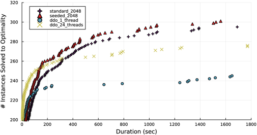
TSPTW Instances Solved over Time: DDO vs. Peel-and-Bound

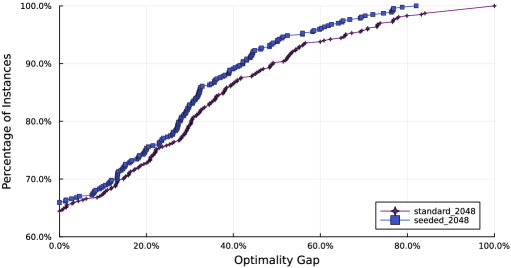
TSPTW Performance Profiles

Figure 8: Performance of Peel-and-Bound on TSPTW.

It is clear from Figure 8, that peel-and-bound outperforms ddo on the TSPTW benchmark set. Although ddo is faster to start, peel-and-bound on a single thread solves about 60 more instances than ddo on a single thread, and about 20 more instances than ddo using 24 threads. This experiment plainly demonstrates the advantages of trading memory for speed when using decision diagrams. The performance profiles show that peel-and-bound solved about $65\%$ of the instances to optimality. The seeded version of the solver performed only slightly better. Looking at the raw data (available in the repository), it is also clear that performance degrades when peel-and-bound has trouble finding good solutions, and when the size of the time windows is large (causing the problem to be more unconstrained than others in the benchmark set).

To the best of our knowledge, the last paper to report relaxed bounds on the instances in these benchmark sets is Baldacci et al. (2012). So we compare our results to Baldacci et al. (2012). The standard run of the solver closes 14 instances that were left open by Baldacci et al. (2012), and the seeded run of the solver closes one additional instance. The results for these instances, and the best relaxed bound found by Baldacci et al. (2012), are reported in Table 3. A table with every problem from the benchmark set that remains open to the best of our knowledge (in other words, those unsolved by both Baldacci et al. (2012) and peel-and-bound), is available in Appendix A: Table 8. The full data is available in Appendix A: Tables 10-15. The raw data is also available in the repository with the solver.

Problem Information			Baldacci et al. (2012)	Single Thread: 2048				Seeded Single Thread: 2048
Set	Name	Best Known Solution	LB	LB	UB	Time	OG	LB	UB	Time	OG
AFG	rbg086a.tw	8400	8399	8400	8400	254.47	-	8400	8400	132.49	-
	rbg092a.tw	7158	7156.6	7158	7158	1917.74	-	7158	7158	288.02	-
GendreauDumas	n20w200.004.txt	293	289.484	293	293	27.97	-	293	293	15.47	-
	n40w200.002.txt	303	302.091	303	303	1388.47	-	303	303	417.75	-
	n80w100.004.txt	649	645.408	649	649	2372.02	-	649	649	904.33	-
SolomonPesant	rc203.1	726.99	726.66	726.99	726.99	299.58	-	726.99	726.99	200.01	-
SolomonPotvinBengio	rc_202.3.txt	837.72	835.87	837.72	837.72	9.66	-	837.72	837.72	8.67	-
	rc_202.4.txt	793.03	791.54	793.03	793.03	108.08	-	793.03	793.03	73.79	-
	rc_205.4.txt	760.47	756.95	760.47	760.47	13.65	-	760.47	760.47	9.74	-
	rc_206.2.txt	828.06	826.66	828.06	828.06	102.63	-	828.06	828.06	68.91	-
	rc_206.4.txt	831.67	827.54	831.67	831.67	107.39	-	831.67	831.67	84.51	-
	rc_207.1.txt	732.68	731.57	732.68	732.68	195.9	-	732.68	732.68	157.17	-
	rc_207.2.txt	701.25	694.22	701.25	701.25	1690.43	-	701.25	701.25	92.84	-
	rc_207.3.txt	682.40	677.23	682.40	682.40	1054.62	-	682.40	682.40	596.7	-
	rc_208.1.txt	789.25	785.69	751.20	794.17	-	5.41	789.25	789.25	2511.58	-

Table 3: TSPTW Results for Newly Closed Problems: LB = Lower Bound, UB = Upper Bound, OG = Optimality Gap. In all cases the existing best known solution was proven optimal by Peel and Bound.

5.3 Traveling Salesman Problem with Time Windows - Makespan

Makespan adjusts the objective function of TSPTW so the total time includes any idle time spent waiting for a customer to be available when the salesman arrives early, as opposed to just the distance traveled. To test this problem, we use the same benchmark instances that we did in Section 5.2, and simply adjust the objective function. The tests all use the same settings as the test for TSPTW, and the results are presented in the same way in Figure 9.

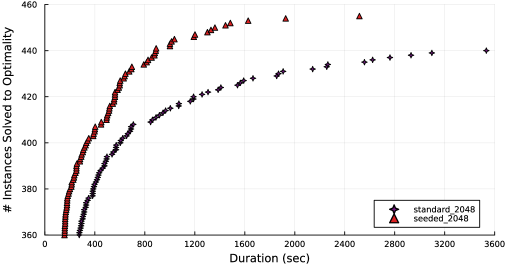
Makespan Instances Solved over Time

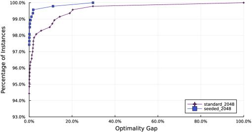
Makespan Performance Profiles

Figure 9: Performance of Peel-and-Bound on Makespan.

While we were unable to find a a benchmark comparison in the literature with relaxed bounds for the makespan variant of these benchmark sets, the results from testing peel-and-bound on makespan speak for themselves. Just over $94\%$ of the instances were closed to optimality by the unseeded run of the solver, and just over $97\%$ were closed by the seeded run. For the unseeded run, just over $97.5\%$ were closed to $1\%$ optimality gap, and $99\%$ for the seeded run. In total, 26 instances were not closed by the unseeded run, and 12 of those were not closed by the seeded run. The results and bounds for those 26 instances are shown in Table 4. We are unsure if any of the makespan problems are considered to be open, but we can say that the only ones that aren’t definitively closed are the 12 not in bold that were not solved during the seeded run of the solver. Of those, only 2 have an optimality gap larger than $2\%$. For the 455 closed instances, the best solution found was the best solution reported by López-Ibáñez & Blum (2022). A table with full results for the benchmark sets, and time to solve for all of the closed problems, is shown in Appendix A: Tables 16-22. The raw data is also available in the repository with the solver.

Problem Information			Single Thread: 2048			Seeded Single Thread: 2048
Set	Name	Best Known Solution	LB	UB	OG	LB	UB	OG
AFG	rbg050b.tw	11957	11748	11957	1.75	11748	11957	1.75
	rbg172a.tw	17783	17766	17784	0.10	17766	17783	0.10
Dumas	n150w60.002.txt	940	940	941	0.11	940	940	-
	n200w40.002.txt	1137	1137	-	100	1137	1137	-
GendreauDumas	n100w100.003.txt	819	818	819	0.12	818	819	0.12
	n100w80.003.txt	829	829	839	1.19	829	829	-
	n60w200.003.txt	560	560	561	0.18	560	560	-
	n80w140.005.txt	739	725	739	1.89	725	739	1.89
	n80w160.002.txt	654	652	665	1.95	654	654	-
	n80w180.002.txt	633	631	639	1.25	631	633	0.32
	n80w180.005.txt	632	444	632	29.75	444	632	29.75
	n80w200.004.txt	667	660	671	1.64	660	667	1.05
OhlmannThomas	n150w120.004.txt	925	925	929	0.43	925	925	-
	n150w140.002.txt	1020	1020	1021	0.10	1020	1020	-
	n150w140.004.txt	898	898	919	2.29	898	898	-
	n150w140.005.txt	926	826	926	10.8	926	926	-
	n150w160.002.txt	890	861	912	5.59	890	890	-
	n150w160.004.txt	912	912	943	3.29	912	912	-
	n200w120.001.txt	1089	1086	1089	0.28	1086	1089	0.28
	n200w120.002.txt	1072	1065	1072	0.65	1065	1072	0.65
	n200w140.001.txt	1138	929	1146	18.94	1138	1138	-
	n200w140.003.txt	1083	979	1083	9.60	1082	1083	0.09
	n200w140.005.txt	1121	961	1121	14.27	1121	1121	-
SolomonPesant	rc204.2	870.52	728.94	914.89	20.33	870.52	870.52	-
SolomonPotvinBengio	rc_204.1.txt	917.83	915.22	918.01	0.30	915.22	917.83	0.28
	rc_208.3.txt	686.80	606.15	686.80	11.74	610.58	686.80	11.10

Table 4: Makespan Results for Problems Not Closed by the Unseeded Run: LB = Lower Bound, UB = Upper Bound, OG = Optimality Gap. The bolded instances were closed by the seeded run.

6 Conclusion and Future Work

This paper presented a peel-and-bound algorithm as an alternative to branch-and-bound. In peel-and-bound, constructed decision diagrams are repeatedly reused to avoid unnecessary computation. Additionally, peel-and-bound can be used in combination with a decision diagram structure that only admits exact arc values, to increase scalability and further reduce the amount of work needed at each iteration of the algorithm. We identified several heuristic decisions that can be used to adjust peel-and-bound, and provided insight into how the algorithm can be applied to other problems.

We compared the performance of a peel-and-bound scheme to a branch-and-bound scheme using the same DD based propagator. We tested both algorithms on the 41 instances of the SOP from TSPLIB. Results show that peel-and-bound significantly outperforms branch-and-bound on the SOP by generating substantially stronger relaxed bounds on instances that were not closed during the experiment, and reaching optimality faster when the instances were closed. We then re-implemented the algorithm to be more efficient, and generic. We tested the new implementation on the 467 benchmark instances of TSPTW used by Gillard et al. (2021) to test their decision diagram based branch-and-bound solver (ddo). The results show that peel-and-bound outperforms ddo on TSPTW, even when ddo is using parallel processing. Furthermore, peel-and-bound closed 16 instances that, to the best of our knowledge, are open in the literature. In our final test, we ran the new implementation of peel-and-bound on the makespan variant of the 467 TSPTW instances. Peel-and-bound closed $94\%$ of the makespan instances, and an additional $3\%$ when seeded with the best known solution. We provide best known bounds for all TSPTW and makespan instances that we believe to be open.

This paper provides strong support for the value of re-using work in DD based solvers. Furthermore, peel-and-bound benefits from scaling the maximum allowable width. Thus, relaxed DDs that yield strong bounds at scale, but are too costly to generate iteratively, only need to be constructed once. The method detailed in this paper focused on DDs generated by separation; future research could focus on DDs generated using a merge operator.

A Experimental Data

Problem Info		BnB: width 64					PnB: width 64					Percent Improvements
Name	n	RB	BS	T	OG	QL	RB	BS	T	OG	QL	RB	BS	T	OG	QL
ESC07	9	2,125	2,125	0.03	0%	-	2,125	2,125	0.07	0%	-			-57%
ESC11	13	2,075	2,075	0.65	0%	-	2,075	2,075	0.42	0%	-			55%
ESC12	14	1,675	1,675	1.99	0%	-	1,675	1,675	0.64	0%	-			211%
ESC25	27	1,681	1,681	956	0%	-	1,681	1,681	353	0%	-			171%
ESC47	49	334	1,542		78%	8,842	368	1,676		78%	1,295	10.2%	-8.0%		0.4%	583%
ESC63	65	8	62		87%	2,756	44	62		29%	15	450.0%	0.0%		200.0%	18273%
ESC78	80	2,230	19,800		89%	1,040	5,000	20,045		75%	316	124.2%	-1.2%		18.2%	229%
br17.10	18	55	55	260	0%	-	55	55	5	0%	-			4652%
br17.12	18	55	55	138	0%	-	55	55	21	0%	-			546%
ft53.1	54	1,785	8,478		79%	8,841	3,324	8,244		60%	917	86.2%	2.8%		32.3%	864%
ft53.2	54	1,946	8,927		78%	7,356	3,450	8,633		60%	938	77.3%	3.4%		30.3%	684%
ft53.3	54	2,546	12,179		79%	5,594	4,234	12,327		66%	1,147	66.3%	-1.2%		20.5%	388%
ft53.4	54	3,780	14,811		74%	11,907	6,500	14,753		56%	2,372	72.0%	0.4%		33.1%	402%
ft70.1	71	25,444	41,926		39%	4,781	31,123	41,607		25%	412	22.3%	0.8%		56.0%	1060%
ft70.2	71	25,239	42,805		41%	3,998	31,195	42,623		27%	427	23.6%	0.4%		53.1%	836%
ft70.3	71	25,810	48,073		46%	4,036	31,872	47,491		33%	475	23.5%	1.2%		40.8%	750%
ft70.4	71	28,593	56,644		50%	8,642	35,974	56,552		36%	1,087	25.8%	0.2%		36.1%	695%
kro124p.1	101	10,773	46,158		77%	2,173	17,579	46,158		62%	105	63.2%	0.0%		23.8%	1970%
kro124p.2	101	11,061	46,930		76%	1,898	17,633	46,930		62%	109	59.4%	0.0%		22.4%	1641%
kro124p.3	101	12,110	55,991		78%	1,055	18,586	55,991		67%	117	53.5%	0.0%		17.3%	802%
kro124p.4	101	13,838	85,533		84%	2,990	24,388	85,316		71%	244	76.2%	0.3%		17.4%	1125%
p43.1	44	630	29,450		98%	12,945	380	29,380		99%	1,022	-39.7%	0.2%		-0.9%	1167%
p43.2	44	440	29,000		98%	8,519	420	29,080		99%	1,125	-4.5%	-0.3%		-0.1%	657%
p43.3	44	595	29,530		98%	12,802	490	29,530		98%	1,122	-17.6%	0.0%		-0.4%	1041%
p43.4	44	1,370	83,855		98%	21,105	1,050	83,890		99%	4,694	-23.4%	0.0%		-0.4%	350%
prob.42	42	99	289		66%	16,742	97	286		66%	2,613	-2.0%	1.0%		-0.5%	541%
prob.100	100	170	1,841		91%	1,731	182	1,760		90%	117	7.1%	4.6%		1.2%	1379%
rbg048a	50	76	379		80%	12,938	47	380		88%	1,551	-38.2%	-0.3%		-8.8%	734%
rbg050c	52	63	566		89%	11,480	154	512		70%	1,481	144.4%	10.5%		27.1%	675%
rbg109a	111	91	1,196		92%	2,773	379	1,196		68%	612	316.5%	0.0%		35.3%	353%
rbg150a	152	63	1,874		97%	241	565	1,865		70%	222	796.8%	0.5%		38.6%	9%
rbg174a	176	119	2,157		94%	809	626	2,156		71%	117	426.1%	0.0%		33.1%	591%
rbg253a	255	113	3,181		96%	403	708	3,180		78%	39	526.5%	0.0%		24.1%	933%
rbg323a	325	89	3,519		97%	437	289	3,529		92%	17	224.7%	-0.3%		6.2%	2471%
rbg341a	343	68	3,038		98%	366	321	3,064		90%	8	372.1%	-0.8%		9.2%	4475%
rbg358a	360	69	3,359		98%	289	73	3,373		98%	6	5.8%	-0.4%		0.1%	4717%
rbg378a	380	52	3,429		98%	266	50	3,429		99%	5	-3.8%	0.0%		-0.1%	5220%
ry48p.1	49	5,201	17,555		70%	10,480	6,171	17,454		65%	1,395	18.7%	0.6%		8.9%	651%
ry48p.2	49	5,291	18,046		71%	9,286	6,577	17,840		63%	1,445	24.3%	1.2%		12.0%	543%
ry48p.3	49	6,207	21,161		71%	9,039	6,985	20,962		67%	1,707	12.5%	0.9%		6.0%	430%
ry48p.4	49	13,610	34,517		61%	15,819	14,293	33,804		58%	3,217	5.0%	2.1%		4.9%	392%

Table 5: Comparison Data for width 64 experiments on SOP: RB = Relaxed Bound, BS = Best Solution, T = Time in Seconds, OG = Optimality Gap, QL = Queue Length. Full time series data is available in the GitHub repository.

Problem Info		BnB: width 256					PnB: width 256					Percent Improvements
Name	n	RB	BS	T	OG	QL	RB	BS	T	OG	QL	RB	BS	T	OG	QL
ESC07	9	2,125	2,125	0.04	0%	-	2,125	2,125	0.04	0%	-			0%
ESC11	13	2,075	2,075	0.48	0%	-	2,075	2,075	0.41	0%	-			17%
ESC12	14	1,675	1,675	1.66	0%	-	1,675	1,675	0.34	0%	-			388%
ESC25	27	1,681	1,681	2,643	0%	-	1,681	1,681	303	0%	-			771%
ESC47	49	312	1,590		80%	720	658	1,339		51%	740	110.9%	18.7%		58.0%	-3%
ESC63	65	9	62		85%	53	44	62		29%	3	388.9%	0.0%		194.4%	1667%
ESC78	80	2,230	20,345		89%	59	5,600	20,135		72%	109	151.1%	1.0%		23.3%	-46%
br17.10	18	55	55	275	0%	-	55	55	3	0%	-			9468%
br17.12	18	55	55	105	0%	-	55	55	5	0%	-			2146%
ft53.1	54	1,708	8,424		80%	760	4,603	8,244		44%	271	169.5%	2.2%		80.5%	180%
ft53.2	54	1,856	9,059		80%	632	3,555	8,648		59%	272	91.5%	4.8%		35.0%	132%
ft53.3	54	2,493	12,598		80%	477	4,852	11,095		56%	390	94.6%	13.5%		42.6%	22%
ft53.4	54	3,619	14,867		76%	1,240	7,560	14,611		48%	797	108.9%	1.8%		56.8%	56%
ft70.1	71	25,507	41,686		39%	373	31,122	41,235		25%	108	22.0%	1.1%		58.3%	245%
ft70.2	71	25,261	42,901		41%	297	31,630	42,182		25%	123	25.2%	1.7%		64.4%	141%
ft70.3	71	25,891	47,806		46%	377	32,539	46,488		30%	151	25.7%	2.8%		52.8%	150%
ft70.4	71	31,186	56,366		45%	958	37,984	56,366		33%	356	21.8%	0.0%		37.0%	169%
kro124p.1	101	10,683	48,866		78%	152	19,224	45,643		58%	43	79.9%	7.1%		35.0%	253%
kro124p.2	101	10,706	52,038		79%	125	19,299	48,102		60%	43	80.3%	8.2%		32.6%	191%
kro124p.3	101	12,078	58,562		79%	64	20,145	57,358		65%	45	66.8%	2.1%		22.3%	42%
kro124p.4	101	14,511	82,672		82%	281	25,002	82,364		70%	102	72.3%	0.4%		18.4%	175%
p43.1	44	610	29,460		98%	1,033	27,255	28,635		5%	146	4368%	2.9%		1932%	608%
p43.2	44	460	29,020		98%	547	27,455	29,020		5%	391	5868%	0.0%		1725%	40%
p43.3	44	750	29,530		97%	1,016	27,780	29,530		6%	764	3604%	0.0%		1545%	33%
p43.4	44	1,425	83,880		98%	1,365	28,195	83,435		66%	1,380	1879%	0.5%		48.5%	-1%
prob.42	42	90	289		69%	1,166	103	275		63%	617	14.4%	5.1%		10.1%	89%
prob.100	100	157	1,886		92%	113	178	1,721		90%	45	13.4%	9.6%		2.3%	151%
rbg048a	50	80	389		79%	794	80	373		79%	534	0.0%	4.3%		1.1%	49%
rbg050c	52	62	583		89%	810	175	503		65%	442	182.3%	15.9%		37.0%	83%
rbg109a	111	89	1,181		92%	394	406	1,106		63%	204	356.2%	6.8%		46.1%	93%
rbg150a	152	115	1,845		94%	406	571	1,845		69%	100	396.5%	0.0%		35.8%	306%
rbg174a	176	362	2,172		83%	337	646	2,171		70%	57	78.5%	0.0%		18.6%	491%
rbg253a	255	359	3,177		89%	139	727	3,176		77%	22	102.5%	0.0%		15.0%	532%
rbg323a	325	99	3,476		97%	114	346	3,480		90%	14	249.5%	-0.1%		7.9%	714%
rbg341a	343	84	3,016		97%	120	340	3,016		89%	7	304.8%	0.0%		9.6%	1614%
rbg358a	360	88	3,280		97%	92	88	3,382		97%	5	0.0%	-3.0%		-0.1%	1740%
rbg378a	380	44	3,385		99%	35	53	3,385		98%	6	20.5%	0.0%		0.3%	483%
ry48p.1	49	5,470	17,464		69%	897	9,432	17,071		45%	377	72.4%	2.3%		53.5%	138%
ry48p.2	49	5,606	18,060		69%	834	6,615	17,627		62%	383	18.0%	2.5%		10.4%	118%
ry48p.3	49	6,558	21,142		69%	859	8,723	20,850		58%	513	33.0%	1.4%		18.6%	67%
ry48p.4	49	17,359	34,074		49%	1,557	17,322	33,773		49%	990	-0.2%	0.9%		0.7%	57%

Table 6: Comparison data for width 256 experiments on SOP: RB = Relaxed Bound, BS = Best Solution, T = Time in Seconds, OG = Optimality Gap, QL = Queue Length. Full time series data is available in the GitHub repository.

Problem Info		PnB: width 256			PnB: width 2048			Percent Improvements
Name	n	RB	BS	OG	RB	BS	OG	RB	BS	OG
ESC47	49	658	1,339	51%	882	1,304	32%	34.0%	2.7%	57.2%
ESC63	65	44	62	29%	44	62	29%	0.0%	0.0%	0%
ESC78	80	5,600	20,135	72%	6,025	20,505	71%	7.6%	-1.8%	2.2%
ft53.1	54	4,603	8,244	44%	5,167	8,237	37%	12.3%	0.1%	18.5%
ft53.2	54	3,555	8,648	59%	4,910	8,598	43%	38.1%	0.6%	37.3%
ft53.3	54	4,852	11,095	56%	7,722	11,092	30%	59.2%	0.0%	85.2%
ft53.4	54	7,560	14,611	48%	7,466	14,618	49%	-1.2%	0.0%	-1.4%
ft70.1	71	31,122	41,235	25%	33,382	41,476	20%	7.3%	-0.6%	25.7%
ft70.2	71	31,630	42,182	25%	32,964	41,833	21%	4.2%	0.8%	18.0%
ft70.3	71	32,539	46,488	30%	34,366	46,001	25%	5.6%	1.1%	18.6%
ft70.4	71	37,984	56,366	33%	40,919	56,310	27%	7.7%	0.1%	19.3%
kro124p.1	101	19,224	45,643	58%	21,954	47,425	54%	14.2%	-3.8%	7.8%
kro124p.2	101	19,299	48,102	60%	22,746	49,571	54%	17.9%	-3.0%	10.7%
kro124p.3	101	20,145	57,358	65%	25,566	54,633	53%	26.9%	5.0%	21.9%
kro124p.4	101	25,002	82,364	70%	29,377	81,050	64%	17.5%	1.6%	9.2%
p43.1	44	27,255	28,635	5%	27,755	28,960	4%	1.8%	-1.1%	16%
p43.2	44	27,455	29,020	5%	27,725	29,000	4%	1.0%	0.1%	23%
p43.3	44	27,780	29,530	6%	27,755	29,530	6%	-0.1%	0.0%	-1%
p43.4	44	28,195	83,435	66%	28,680	83,020	65%	1.7%	0.5%	1.2%
prob.42	42	103	275	63%	152	261	42%	47.6%	5.4%	49.8%
prob.100	100	178	1,721	90%	220	1,735	87%	23.6%	-0.8%	2.7%
rbg048a	50	80	373	79%	93	367	75%	16.3%	1.6%	5.2%
rbg050c	52	175	503	65%	184	501	63%	5.1%	0.4%	3.1%
rbg109a	111	406	1,106	63%	453	1,126	60%	11.6%	-1.8%	5.9%
rbg150a	152	571	1,845	69%	672	1,841	63%	17.7%	0.2%	8.7%
rbg174a	176	646	2,171	70%	1,104	2,121	48%	70.9%	2.4%	46.5%
rbg253a	255	727	3,176	77%	1,186	3,101	62%	63.1%	2.4%	24.9%
rbg323a	325	346	3,480	90%	421	3,449	88%	21.7%	0.9%	2.6%
rbg341a	343	340	3,016	89%	329	2,965	89%	-3.2%	1.7%	-0.2%
rbg358a	360	88	3,382	97%	107	3,131	97%	21.6%	8.0%	0.8%
rbg378a	380	53	3,385	98%	74	3,338	98%	39.6%	1.4%	0.7%
ry48p.1	49	9,432	17,071	45%	10,386	17,124	39%	10.1%	-0.3%	13.7%
ry48p.2	49	6,615	17,627	62%	7,896	17,461	55%	19.4%	1.0%	14.0%
ry48p.3	49	8,723	20,850	58%	10,558	20,686	49%	21.0%	0.8%	18.8%
ry48p.4	49	17,322	33,773	49%	24,248	32,953	26%	40.0%	2.5%	84.4%

Table 7: Comparison of PnB at 2048 over PnB at 256 on SOP: RB = Relaxed Bound, BS = Best Solution, OG = Optimality Gap.

Problem Information			Baldacci et. al. (2012)	Single Thread: 2048			Seeded Single Thread: 2048
Set	Name	Best Known Solution	LB	LB	UB	OG	LB	UB	OG
Dumas	n100w60.001.txt	655	NA	602	659	8.65	602	655	8.09
Dumas	n100w60.003.txt	744	NA	619	749	17.36	620	744	16.67
Dumas	n100w60.004.txt	764	NA	657	-	100.00	656	764	14.14
Dumas	n150w40.001.txt	918	NA	810	919	11.86	812	918	11.55
Dumas	n150w40.002.txt	941	NA	804	945	14.92	803	941	14.67
Dumas	n150w40.003.txt	727	NA	528	737	28.36	525	727	27.79
Dumas	n150w40.004.txt	764	NA	678	782	13.30	678	764	11.26
Dumas	n150w40.005.txt	824	NA	585	-	100.00	566	824	31.31
Dumas	n150w60.001.txt	859	NA	645	906	28.81	635	859	26.08
Dumas	n150w60.002.txt	782	NA	530	829	36.07	529	782	32.35
Dumas	n150w60.003.txt	793	NA	541	825	34.42	540	793	31.90
Dumas	n150w60.004.txt	819	NA	578	-	100.00	574	819	29.91
Dumas	n150w60.005.txt	840	NA	581	849	31.57	570	840	32.14
Dumas	n200w40.001.txt	1023	NA	643	1038	38.05	638	1023	37.63
Dumas	n200w40.002.txt	948	NA	605	983	38.45	605	948	36.18
Dumas	n200w40.003.txt	933	NA	645	-	100.00	568	933	39.12
Dumas	n200w40.004.txt	980	NA	731	1030	29.03	714	980	27.14
Dumas	n200w40.005.txt	1037	NA	659	1056	37.59	607	1037	41.47
Dumas	n60w100.005.txt	451	NA	390	460	15.22	391	451	13.3
Dumas	n80w80.002.txt	592	NA	508	605	16.03	506	592	14.53
Dumas	n80w80.003.txt	589	NA	500	598	16.39	500	589	15.11
Dumas	n80w80.004.txt	594	NA	506	620	18.39	505	594	14.98
OhlmannThomas	n150w120.001.txt	734	725.50	324	809	59.95	324	734	55.86
OhlmannThomas	n150w120.002.txt	677	668.40	209	717	70.85	209	677	69.13
OhlmannThomas	n150w120.003.txt	747	746.40	416	807	48.45	416	747	44.31
OhlmannThomas	n150w120.004.txt	763	761.60	381	835	54.37	381	763	50.07
OhlmannThomas	n150w120.005.txt	689	684.70	266	754	64.72	274	689	60.23
OhlmannThomas	n150w140.001.txt	762	754.00	394	893	55.88	394	762	48.29
OhlmannThomas	n150w140.002.txt	755	752.00	407	855	52.40	416	755	44.90
OhlmannThomas	n150w140.003.txt	613	608.50	215	738	70.87	215	613	64.93
OhlmannThomas	n150w140.005.txt	663	662.00	197	750	73.73	197	663	70.29
OhlmannThomas	n150w160.001.txt	706	701.40	293	777	62.29	293	706	58.50
OhlmannThomas	n150w160.002.txt	711	709.70	286	826	65.38	286	711	59.77
OhlmannThomas	n150w160.003.txt	608	603.20	170	772	77.98	170	608	72.04
OhlmannThomas	n150w160.004.txt	672	672.00	336	749	55.14	344	672	48.81
OhlmannThomas	n150w160.005.txt	658	655.00	320	736	56.52	320	658	51.37
OhlmannThomas	n200w120.001.txt	799	793.30	312	910	65.71	312	799	60.95
OhlmannThomas	n200w120.002.txt	721	713.90	184	822	77.62	184	721	74.48
OhlmannThomas	n200w120.003.txt	880	868.60	336	983	65.82	336	880	61.82
OhlmannThomas	n200w120.004.txt	777	775.80	291	887	67.19	291	777	62.55
OhlmannThomas	n200w120.005.txt	841	833.20	258	960	73.12	371	841	55.89
OhlmannThomas	n200w140.001.txt	834	826.20	177	1053	83.19	177	834	78.78
OhlmannThomas	n200w140.002.txt	760	756.20	180	895	79.89	180	760	76.32
OhlmannThomas	n200w140.003.txt	758	756.00	241	897	73.13	252	758	66.75
OhlmannThomas	n200w140.004.txt	816	807.10	284	932	69.53	284	816	65.20
OhlmannThomas	n200w140.005.txt	822	819.60	148	927	84.03	148	822	82.00
SolomonPesant	rc203.0	727.45	726.22	608.28	734.00	17.13	608.24	727.45	16.39
SolomonPesant	rc204.2	778.40	774.77	667.18	905.93	26.35	685.22	778.40	11.97

Table 8: (Part 1 of 2) TSPTW Results of PnB at 2048 on open problems: Seeded and Unseeded: LB = Lower Bound, UB = Upper Bound, OG = Optimality Gap.

Problem Information			Baldacci et. al. (2012)	Single Thread: 2048			Seeded Single Thread: 2048
Set	Name	Best Known Solution	LB	LB	UB	OG	LB	UB	OG
AFG	rbg049a.tw	10018	10006.10	9877	10034	1.56	9877	10018	1.41
AFG	rbg050b.tw	9863	9855.80	9711	9876	1.67	9713	9863	1.52
AFG	rbg050c.tw	10024	10020.40	9745	10074	3.27	9746	10024	2.77
AFG	rbg132.2.tw	8192	8188.20	6701	8316	19.42	6695	8192	18.27
AFG	rbg152.3.tw	9788	9785.20	7240	9982	27.47	7240	9788	26.03
AFG	rbg193.2.tw	12142	12136.30	9755	12441	21.59	9755	12142	19.66
GendreauDumas	n100w100.004.txt	684	680.58	484	738	34.42	485	684	29.09
GendreauDumas	n100w120.002.txt	540	535.68	279	581	51.98	279	540	48.33
GendreauDumas	n100w120.004.txt	663	660.01	383	713	46.28	383	663	42.23
GendreauDumas	n100w140.005.txt	509	504.42	346	571	39.40	346	509	32.02
GendreauDumas	n100w160.002.txt	532	528.94	287	601	52.25	286	532	46.24
GendreauDumas	n100w160.005.txt	586	585.41	327	642	49.07	327	586	44.20
GendreauDumas	n100w80.002.txt	668	666.00	542	681	20.41	549	668	17.81
GendreauDumas	n40w180.004.txt	354	352.58	280	359	22.01	283	354	20.06
GendreauDumas	n40w200.003.txt	339	322.05	305	340	10.29	305	339	10.03
GendreauDumas	n40w200.004.txt	301	300.10	232	301	22.92	229	301	23.92
GendreauDumas	n60w140.001.txt	423	421.31	331	425	22.12	332	423	21.51
GendreauDumas	n60w140.002.txt	462	461.08	394	469	15.99	400	462	13.42
GendreauDumas	n60w140.005.txt	460	455.40	334	462	27.71	335	460	27.17
GendreauDumas	n60w160.001.txt	560	556.08	457	572	20.10	457	560	18.39
GendreauDumas	n60w160.003.txt	434	432.70	212	464	54.31	212	434	51.15
GendreauDumas	n60w180.001.txt	411	407.30	234	460	49.13	234	411	43.07
GendreauDumas	n60w180.003.txt	445	440.00	314	458	31.44	314	445	29.44
GendreauDumas	n60w180.004.txt	456	455.54	272	490	44.49	272	456	40.35
GendreauDumas	n60w180.005.txt	395	388.68	274	409	33.01	274	395	30.63
GendreauDumas	n60w200.003.txt	455	444.08	319	471	32.27	321	455	29.45
GendreauDumas	n60w200.004.txt	431	429.71	343	441	22.22	347	431	19.49
GendreauDumas	n60w200.005.txt	427	425.29	292	449	34.97	292	427	31.62
GendreauDumas	n80w120.001.txt	498	497.50	362	514	29.57	362	498	27.31
GendreauDumas	n80w120.002.txt	577	576.42	415	587	29.30	416	577	27.90
GendreauDumas	n80w120.004.txt	501	491.48	301	509	40.86	301	501	39.92
GendreauDumas	n80w120.005.txt	591	586.86	415	594	30.13	415	591	29.78
GendreauDumas	n80w140.002.txt	470	469.06	346	528	34.47	347	470	26.17
GendreauDumas	n80w140.003.txt	580	574.78	297	636	53.30	295	580	49.14
GendreauDumas	n80w140.004.txt	423	420.31	262	449	41.65	262	423	38.06
GendreauDumas	n80w160.002.txt	549	547.45	197	638	69.12	197	549	64.12
GendreauDumas	n80w180.001.txt	551	550.45	373	560	33.39	373	551	32.30
GendreauDumas	n80w200.001.txt	490	486.57	150	555	72.97	150	490	69.39
GendreauDumas	n80w200.002.txt	488	487.51	270	572	52.80	271	488	44.47
GendreauDumas	n80w200.003.txt	464	462.14	194	495	60.81	194	464	58.19
GendreauDumas	n80w200.004.txt	526	521.27	291	565	48.50	292	526	44.49
GendreauDumas	n80w200.005.txt	439	438.12	235	484	51.45	235	439	46.47
SolomonPotvinBengio	rc_203.2.txt	784.16	781.64	659.63	784.16	15.88	658.22	784.16	16.06
SolomonPotvinBengio	rc_203.3.txt	817.53	810.46	735.91	823.44	10.63	756.34	817.53	7.48
SolomonPotvinBengio	rc_204.1.txt	878.64	872.62	791.45	889.53	11.03	794.15	878.64	9.62
SolomonPotvinBengio	rc_204.2.txt	662.16	650.94	525.69	664.52	20.89	526.72	662.16	20.45
SolomonPotvinBengio	rc_208.3.txt	634.44	622.48	549.17	670.56	18.10	550.15	634.44	13.29

Table 9: (Part 2 of 2) TSPTW Results of PnB at 2048 on open problems: Seeded and Unseeded: LB = Lower Bound, UB = Upper Bound, OG = Optimality Gap.

Problem Information			Baldacci et. al. (2012)	Single Thread: 2048				Seeded Single Thread: 2048
Set	Name	Best Known Solution	LB	LB	UB	OG	Time	LB	UB	OG	Time
AFG	rbg010a.tw	671	O	671	671	0	0.08	671	671	0	0.26
AFG	rbg016a.tw	938	O	938	938	0	0.22	938	938	0	0.28
AFG	rbg016b.tw	1304	O	1304	1304	0	5.62	1304	1304	0	4.43
AFG	rbg017.2.tw	852	O	852	852	0	9.08	852	852	0	4.71
AFG	rbg017.tw	893	O	893	893	0	3.92	893	893	0	2.96
AFG	rbg017a.tw	4296	O	4296	4296	0	0.28	4296	4296	0	0.22
AFG	rbg019a.tw	1262	O	1262	1262	0	0.21	1262	1262	0	0.19
AFG	rbg019b.tw	1866	O	1866	1866	0	12.96	1866	1866	0	5.67
AFG	rbg019c.tw	4536	O	4536	4536	0	2.91	4536	4536	0	3.64
AFG	rbg019d.tw	1356	O	1356	1356	0	3.66	1356	1356	0	0.37
AFG	rbg020a.tw	4689	O	4689	4689	0	0.22	4689	4689	0	0.23
AFG	rbg021.2.tw	4528	O	4528	4528	0	10.08	4528	4528	0	5.45
AFG	rbg021.3.tw	4528	O	4528	4528	0	15.74	4528	4528	0	7.80
AFG	rbg021.4.tw	4525	O	4525	4525	0	25.67	4525	4525	0	9.71
AFG	rbg021.5.tw	4515	O	4515	4515	0	25.13	4515	4515	0	12.88
AFG	rbg021.6.tw	4480	O	4480	4480	0	2458.01	4480	4480	0	2501.88
AFG	rbg021.7.tw	4479	O	1050	4480	76.56	-	1050	4479	76.56	-
AFG	rbg021.8.tw	4478	O	1042	4480	76.74	-	1041	4478	76.75	-
AFG	rbg021.9.tw	4478	O	1037	4480	76.85	-	1039	4478	76.8	-
AFG	rbg021.tw	4536	O	4536	4536	0	3.11	4536	4536	0	2.81
AFG	rbg027a.tw	5091	O	5091	5091	0	10.69	5091	5091	0	8.34
AFG	rbg031a.tw	1863	O	1863	1863	0	28.16	1863	1863	0	13.51
AFG	rbg033a.tw	2069	O	2069	2069	0	33.44	2069	2069	0	18.26
AFG	rbg034a.tw	2222	O	2222	2222	0	83.72	2222	2222	0	34.02
AFG	rbg035a.2.tw	2056	O	1837	2088	12.02	-	1838	2056	10.6	-
AFG	rbg035a.tw	2144	O	2144	2144	0	44.80	2144	2144	0	28.45
AFG	rbg038a.tw	2480	O	2480	2480	0	75.79	2480	2480	0	17.41
AFG	rbg040a.tw	2378	2376.9	2378	2378	0	57.1	2378	2378	0	36.71
AFG	rbg041a.tw	2598	O	2598	2598	0	109.23	2598	2598	0	81.37
AFG	rbg042a.tw	2772	O	2772	2772	0	154.46	2772	2772	0	88.88
AFG	rbg048a.tw	9383	O	9011	9419	4.33	-	9013	9383	3.94	-
AFG	rbg050a.tw	2953	O	2361	2990	21.04	-	2362	2953	20.01	-
AFG	rbg055a.tw	3761	O	3761	3761	0	405.98	3761	3761	0	121.22
AFG	rbg067a.tw	4625	O	4625	4625	0	634.69	4625	4625	0	158.26
AFG	rbg125a.tw	7936	O	7918	8051	1.65	-	7936	7936	0	2479.97
AFG	rbg132.tw	8468	O	8449	8530	0.95	-	8468	8468	0	549.16
AFG	rbg152.tw	10032	O	10024	10086	0.61	-	10032	10032	0	1011.24
AFG	rbg172a.tw	10950	O	10082	11172	9.76	-	10082	10950	7.93	-
AFG	rbg193.tw	12535	O	11994	12781	6.16	-	11958	12535	4.6	-
AFG	rbg201a.tw	12948	O	11528	13240	12.93	-	11753	12948	9.23	-
AFG	rbg233.2.tw	14495	O	11634	14827	21.54	-	11634	14495	19.74	-
AFG	rbg233.tw	14992	O	13355	15330	12.88	-	12988	14992	13.37	-
Dumas	n100w20.001.txt	738	NA	738	738	0	32.87	738	738	0	5.06
Dumas	n100w20.002.txt	715	NA	715	715	0	64.56	715	715	0	30.67
Dumas	n100w20.003.txt	762	NA	762	762	0	49.73	762	762	0	42.79
Dumas	n100w20.004.txt	799	NA	799	799	0	51.93	799	799	0	28.00
Dumas	n100w20.005.txt	774	NA	774	774	0	45.66	774	774	0	35.66
Dumas	n100w40.001.txt	770	NA	770	770	0	178.71	770	770	0	129.09
Dumas	n100w40.002.txt	653	NA	653	653	0	573.14	653	653	0	455.42
Dumas	n100w40.003.txt	736	NA	736	736	0	390.53	736	736	0	341.37
Dumas	n100w40.004.txt	651	NA	651	651	0	500.63	651	651	0	406.68
Dumas	n100w40.005.txt	699	NA	699	699	0	518.71	699	699	0	455.31
Dumas	n100w60.002.txt	659	NA	659	659	0	1348.85	659	659	0	1503.28
Dumas	n100w60.005.txt	661	NA	661	661	0	1027.05	661	661	0	1054.34
Dumas	n150w20.001.txt	925	NA	925	925	0	380.14	925	925	0	248.27
Dumas	n150w20.002.txt	864	NA	864	864	0	234.78	864	864	0	126.45
Dumas	n150w20.003.txt	834	NA	834	834	0	410.38	834	834	0	305.72
Dumas	n150w20.004.txt	873	NA	873	873	0	343.26	873	873	0	304.33
Dumas	n150w20.005.txt	846	NA	846	846	0	423.04	846	846	0	452.06
Dumas	n200w20.001.txt	1019	NA	1019	1019	0	2739.07	1019	1019	0	2898.58
Dumas	n200w20.002.txt	972	NA	971	1000	2.9	-	972	972	0	614.20
Dumas	n200w20.003.txt	1050	NA	1050	1050	0	1330.33	1050	1050	0	1523.48
Dumas	n200w20.004.txt	984	NA	984	984	0	2360.97	984	984	0	3345.67
Dumas	n200w20.005.txt	1020	NA	1020	1020	0	445.04	1020	1020	0	1059.73
Dumas	n20w100.001.txt	237	NA	237	237	0	7.62	237	237	0	4.32
Dumas	n20w100.002.txt	222	NA	222	222	0	10.21	222	222	0	4.97
Dumas	n20w100.003.txt	310	NA	310	310	0	8.85	310	310	0	4.35
Dumas	n20w100.004.txt	349	NA	349	349	0	2.56	349	349	0	0.70
Dumas	n20w100.005.txt	258	NA	258	258	0	10.40	258	258	0	6.06

Table 10: (Part 1 of 6) TSPTW Results of PnB at 2048 on closed problems: Seeded and Unseeded: LB = Lower Bound, UB = Upper Bound, OG = Optimality Gap, O = Optimality Proved.

Problem Information			Baldacci et. al. (2012)	Single Thread: 2048				Seeded Single Thread: 2048
Set	Name	Best Known Solution	LB	LB	UB	OG	Time	LB	UB	OG	Time
Dumas	n20w20.001.txt	378	NA	378	378	0	0.06	378	378	0	0.18
Dumas	n20w20.002.txt	286	NA	286	286	0	0.08	286	286	0	0.18
Dumas	n20w20.003.txt	394	NA	394	394	0	0.07	394	394	0	0.18
Dumas	n20w20.004.txt	396	NA	396	396	0	0.06	396	396	0	0.18
Dumas	n20w20.005.txt	352	NA	352	352	0	0.07	352	352	0	0.26
Dumas	n20w40.001.txt	254	NA	254	254	0	0.12	254	254	0	0.31
Dumas	n20w40.002.txt	333	NA	333	333	0	0.07	333	333	0	0.24
Dumas	n20w40.003.txt	317	NA	317	317	0	0.07	317	317	0	0.19
Dumas	n20w40.004.txt	388	NA	388	388	0	0.07	388	388	0	0.20
Dumas	n20w40.005.txt	288	NA	288	288	0	0.08	288	288	0	0.20
Dumas	n20w60.001.txt	335	NA	335	335	0	2.22	335	335	0	1.48
Dumas	n20w60.002.txt	244	NA	244	244	0	0.56	244	244	0	0.21
Dumas	n20w60.003.txt	352	NA	352	352	0	0.10	352	352	0	0.22
Dumas	n20w60.004.txt	280	NA	280	280	0	7.50	280	280	0	3.67
Dumas	n20w60.005.txt	338	NA	338	338	0	0.62	338	338	0	0.22
Dumas	n20w80.001.txt	329	NA	329	329	0	2.00	329	329	0	1.37
Dumas	n20w80.002.txt	338	NA	338	338	0	1.27	338	338	0	1.34
Dumas	n20w80.003.txt	320	NA	320	320	0	0.74	320	320	0	0.41
Dumas	n20w80.004.txt	304	NA	304	304	0	1.99	304	304	0	0.90
Dumas	n20w80.005.txt	264	NA	264	264	0	8.19	264	264	0	4.24
Dumas	n40w100.001.txt	429	NA	429	429	0	67.70	429	429	0	68.84
Dumas	n40w100.002.txt	358	NA	358	358	0	84.97	358	358	0	73.49
Dumas	n40w100.003.txt	364	NA	364	364	0	71.79	364	364	0	50.69
Dumas	n40w100.004.txt	357	NA	357	357	0	66.54	357	357	0	58.87
Dumas	n40w100.005.txt	377	NA	377	377	0	82.67	377	377	0	52.66
Dumas	n40w20.001.txt	500	NA	500	500	0	0.51	500	500	0	0.41
Dumas	n40w20.002.txt	552	NA	552	552	0	2.08	552	552	0	0.54
Dumas	n40w20.003.txt	478	NA	478	478	0	1.11	478	478	0	0.34
Dumas	n40w20.004.txt	404	NA	404	404	0	1.19	404	404	0	0.34
Dumas	n40w20.005.txt	499	NA	499	499	0	0.09	499	499	0	0.29
Dumas	n40w40.001.txt	465	NA	465	465	0	2.41	465	465	0	0.61
Dumas	n40w40.002.txt	461	NA	461	461	0	18.31	461	461	0	10.02
Dumas	n40w40.003.txt	474	NA	474	474	0	4.11	474	474	0	1.86
Dumas	n40w40.004.txt	452	NA	452	452	0	13.72	452	452	0	9.67
Dumas	n40w40.005.txt	453	NA	453	453	0	20.16	453	453	0	8.88
Dumas	n40w60.001.txt	494	NA	494	494	0	15.85	494	494	0	16.40
Dumas	n40w60.002.txt	470	NA	470	470	0	24.24	470	470	0	15.00
Dumas	n40w60.003.txt	408	NA	408	408	0	21.72	408	408	0	13.27
Dumas	n40w60.004.txt	382	NA	382	382	0	64.78	382	382	0	51.30
Dumas	n40w60.005.txt	328	NA	328	328	0	32.39	328	328	0	11.37
Dumas	n40w80.001.txt	395	NA	395	395	0	31.40	395	395	0	21.92
Dumas	n40w80.002.txt	431	NA	431	431	0	59.08	431	431	0	52.11
Dumas	n40w80.003.txt	412	NA	412	412	0	28.76	412	412	0	20.84
Dumas	n40w80.004.txt	417	NA	417	417	0	33.35	417	417	0	28.22
Dumas	n40w80.005.txt	344	NA	344	344	0	58.02	344	344	0	47.72
Dumas	n60w100.001.txt	515	NA	515	515	0	1063.65	515	515	0	970.51
Dumas	n60w100.002.txt	538	NA	538	538	0	456.89	538	538	0	453.45
Dumas	n60w100.003.txt	560	NA	560	560	0	361.90	560	560	0	397.47
Dumas	n60w100.004.txt	510	NA	510	510	0	264.85	510	510	0	313.67
Dumas	n60w20.001.txt	551	NA	551	551	0	6.33	551	551	0	2.46
Dumas	n60w20.002.txt	605	NA	605	605	0	4.83	605	605	0	1.78
Dumas	n60w20.003.txt	533	NA	533	533	0	6.45	533	533	0	1.23
Dumas	n60w20.004.txt	616	NA	616	616	0	7.34	616	616	0	1.77
Dumas	n60w20.005.txt	603	NA	603	603	0	4.11	603	603	0	0.64
Dumas	n60w40.001.txt	591	NA	591	591	0	45.45	591	591	0	35.15
Dumas	n60w40.002.txt	621	NA	621	621	0	72.70	621	621	0	63.07
Dumas	n60w40.003.txt	603	NA	603	603	0	51.21	603	603	0	41.32
Dumas	n60w40.004.txt	597	NA	597	597	0	22.87	597	597	0	11.06
Dumas	n60w40.005.txt	539	NA	539	539	0	28.22	539	539	0	15.14
Dumas	n60w60.001.txt	609	NA	609	609	0	77.16	609	609	0	71.60
Dumas	n60w60.002.txt	566	NA	566	566	0	96.04	566	566	0	91.61
Dumas	n60w60.003.txt	485	NA	485	485	0	130.48	485	485	0	124.08
Dumas	n60w60.004.txt	571	NA	571	571	0	106.17	571	571	0	84.95
Dumas	n60w60.005.txt	569	NA	569	569	0	76.37	569	569	0	71.14
Dumas	n60w80.001.txt	458	NA	458	458	0	546.14	458	458	0	444.94
Dumas	n60w80.002.txt	498	NA	498	498	0	147.40	498	498	0	146.75
Dumas	n60w80.003.txt	550	NA	550	550	0	133.79	550	550	0	129.27
Dumas	n60w80.004.txt	566	NA	566	566	0	207.43	566	566	0	178.19

Table 11: (Part 2 of 6) TSPTW Results of PnB at 2048 on closed problems: Seeded and Unseeded: LB = Lower Bound, UB = Upper Bound, OG = Optimality Gap, O = Optimality Proved.

Problem Information			Baldacci et. al. (2012)	Single Thread: 2048				Seeded Single Thread: 2048
Set	Name	Best Known Solution	LB	LB	UB	OG	Time	LB	UB	OG	Time
Dumas	n60w80.005.txt	468	NA	468	468	0	363.20	468	468	0	363.03
Dumas	n80w20.001.txt	616	NA	616	616	0	58.66	616	616	0	31.87
Dumas	n80w20.002.txt	737	NA	737	737	0	30.47	737	737	0	20.49
Dumas	n80w20.003.txt	667	NA	667	667	0	14.48	667	667	0	5.52
Dumas	n80w20.004.txt	615	NA	615	615	0	41.62	615	615	0	32.25
Dumas	n80w20.005.txt	748	NA	748	748	0	23.05	748	748	0	10.52
Dumas	n80w40.001.txt	606	NA	606	606	0	313.45	606	606	0	245.90
Dumas	n80w40.002.txt	618	NA	618	618	0	135.46	618	618	0	132.07
Dumas	n80w40.003.txt	674	NA	674	674	0	109.76	674	674	0	131.28
Dumas	n80w40.004.txt	557	NA	557	557	0	115.15	557	557	0	112.15
Dumas	n80w40.005.txt	695	NA	695	695	0	130.12	695	695	0	126.17
Dumas	n80w60.001.txt	554	NA	554	554	0	237.93	554	554	0	239.36
Dumas	n80w60.002.txt	633	NA	633	633	0	488.91	633	633	0	562.44
Dumas	n80w60.003.txt	651	NA	651	651	0	421.10	651	651	0	404.65
Dumas	n80w60.004.txt	619	NA	619	619	0	319.16	619	619	0	220.47
Dumas	n80w60.005.txt	575	NA	575	575	0	765.78	575	575	0	918.69
Dumas	n80w80.001.txt	624	NA	624	624	0	995.03	624	624	0	919.20
Dumas	n80w80.005.txt	570	NA	570	570	0	285.37	570	570	0	348.52
GendreauDumas	n100w100.001.txt	643	O	467	670	30.3	-	467	643	27.37	-
GendreauDumas	n100w100.002.txt	619	O	480	629	23.69	-	477	619	22.94	-
GendreauDumas	n100w100.003.txt	685	O	474	703	32.57	-	474	685	30.8	-
GendreauDumas	n100w100.005.txt	572	O	365	617	40.84	-	367	572	35.84	-
GendreauDumas	n100w120.001.txt	629	O	405	639	36.62	-	405	629	35.61	-
GendreauDumas	n100w120.003.txt	617	O	451	634	28.86	-	451	617	26.9	-
GendreauDumas	n100w120.005.txt	537	O	306	592	48.31	-	306	537	43.02	-
GendreauDumas	n100w140.001.txt	604	O	393	704	44.18	-	393	604	34.93	-
GendreauDumas	n100w140.002.txt	615	O	403	650	38	-	403	615	34.47	-
GendreauDumas	n100w140.003.txt	481	O	229	494	53.64	-	229	481	52.39	-
GendreauDumas	n100w140.004.txt	533	O	342	570	40	-	343	533	35.65	-
GendreauDumas	n100w160.001.txt	582	O	415	614	32.41	-	416	582	28.52	-
GendreauDumas	n100w160.003.txt	495	O	301	551	45.37	-	302	495	38.99	-
GendreauDumas	n100w160.004.txt	580	O	391	627	37.64	-	392	580	32.41	-
GendreauDumas	n100w80.001.txt	670	O	591	683	13.47	-	591	670	11.79	-
GendreauDumas	n100w80.003.txt	691	O	480	691	30.54	-	480	691	30.54	-
GendreauDumas	n100w80.004.txt	700	O	574	-	100	-	573	700	18.14	-
GendreauDumas	n100w80.005.txt	603	O	416	648	35.8	-	427	603	29.19	-
GendreauDumas	n20w120.001.txt	267	O	267	267	0	14.18	267	267	0	7.09
GendreauDumas	n20w120.002.txt	218	O	218	218	0	13.27	218	218	0	8.66
GendreauDumas	n20w120.003.txt	303	O	303	303	0	11.09	303	303	0	5.49
GendreauDumas	n20w120.004.txt	300	O	300	300	0	9.41	300	300	0	5.67
GendreauDumas	n20w120.005.txt	240	O	240	240	0	12.67	240	240	0	8.52
GendreauDumas	n20w140.001.txt	176	O	176	176	0	11.91	176	176	0	6.26
GendreauDumas	n20w140.002.txt	272	O	272	272	0	11.35	272	272	0	7.76
GendreauDumas	n20w140.003.txt	236	O	236	236	0	13.22	236	236	0	6.43
GendreauDumas	n20w140.004.txt	255	O	255	255	0	12.99	255	255	0	6.01
GendreauDumas	n20w140.005.txt	225	O	225	225	0	10.73	225	225	0	6.15
GendreauDumas	n20w160.001.txt	241	O	241	241	0	14.81	241	241	0	5.58
GendreauDumas	n20w160.002.txt	201	O	201	201	0	11.25	201	201	0	7.81
GendreauDumas	n20w160.003.txt	201	O	201	201	0	10.86	201	201	0	5.00
GendreauDumas	n20w160.004.txt	203	O	203	203	0	19.55	203	203	0	8.33
GendreauDumas	n20w160.005.txt	245	O	245	245	0	13.27	245	245	0	8.35
GendreauDumas	n20w180.001.txt	253	O	253	253	0	11.97	253	253	0	5.78
GendreauDumas	n20w180.002.txt	265	O	265	265	0	16.99	265	265	0	7.46
GendreauDumas	n20w180.003.txt	271	O	271	271	0	18.30	271	271	0	9.70
GendreauDumas	n20w180.004.txt	201	O	201	201	0	17.58	201	201	0	7.11
GendreauDumas	n20w180.005.txt	193	O	193	193	0	32.53	193	193	0	8.59
GendreauDumas	n20w200.001.txt	233	O	233	233	0	20.03	233	233	0	10.08
GendreauDumas	n20w200.002.txt	203	O	203	203	0	25.27	203	203	0	9.63
GendreauDumas	n20w200.003.txt	249	O	249	249	0	21.51	249	249	0	9.40
GendreauDumas	n20w200.005.txt	227	O	227	227	0	21.91	227	227	0	7.87
GendreauDumas	n40w120.001.txt	434	O	434	434	0	91.00	434	434	0	83.12
GendreauDumas	n40w120.002.txt	445	O	445	445	0	141.74	445	445	0	97.37
GendreauDumas	n40w120.003.txt	357	O	357	357	0	881.45	357	357	0	1338.21
GendreauDumas	n40w120.004.txt	303	O	303	303	0	105.54	303	303	0	96.98
GendreauDumas	n40w120.005.txt	350	O	350	350	0	80.86	350	350	0	62.93
GendreauDumas	n40w140.001.txt	328	O	328	328	0	196.16	328	328	0	148.20
GendreauDumas	n40w140.002.txt	383	O	383	383	0	2768.09	383	383	0	2677.04
GendreauDumas	n40w140.003.txt	398	O	398	398	0	125.13	398	398	0	72.96

Table 12: (Part 3 of 6) TSPTW Results of PnB at 2048 on closed problems: Seeded and Unseeded: LB = Lower Bound, UB = Upper Bound, OG = Optimality Gap, O = Optimality Proved.

Problem Information			Baldacci et. al. (2012)	Single Thread: 2048				Seeded Single Thread: 2048
Set	Name	Best Known Solution	LB	LB	UB	OG	Time	LB	UB	OG	Time
GendreauDumas	n40w140.004.txt	342	O	246	342	28.07	-	246	342	28.07	-
GendreauDumas	n40w140.005.txt	371	O	371	371	0	471.26	371	371	0	289.28
GendreauDumas	n40w160.001.txt	348	O	348	348	0	179.81	348	348	0	159.90
GendreauDumas	n40w160.002.txt	337	O	337	337	0	127.84	337	337	0	115.75
GendreauDumas	n40w160.003.txt	346	O	346	346	0	301.12	346	346	0	156.85
GendreauDumas	n40w160.004.txt	288	O	288	288	0	313.23	288	288	0	292.72
GendreauDumas	n40w160.005.txt	315	O	315	315	0	1389.91	315	315	0	704.93
GendreauDumas	n40w180.001.txt	337	O	274	352	22.16	-	337	337	0	2852.42
GendreauDumas	n40w180.002.txt	347	O	347	347	0	689.55	347	347	0	652.55
GendreauDumas	n40w180.003.txt	279	O	196	279	29.75	-	192	279	31.18	-
GendreauDumas	n40w180.005.txt	335	O	237	340	30.29	-	238	335	28.96	-
GendreauDumas	n40w200.001.txt	330	O	208	343	39.36	-	208	330	36.97	-
GendreauDumas	n40w200.005.txt	296	O	239	302	20.86	-	251	296	15.2	-
GendreauDumas	n60w120.001.txt	384	O	274	396	30.81	-	274	384	28.65	-
GendreauDumas	n60w120.002.txt	427	O	371	435	14.71	-	370	427	13.35	-
GendreauDumas	n60w120.003.txt	407	O	304	438	30.59	-	306	407	24.82	-
GendreauDumas	n60w120.004.txt	490	O	425	490	13.27	-	425	490	13.27	-
GendreauDumas	n60w120.005.txt	547	O	498	549	9.29	-	501	547	8.41	-
GendreauDumas	n60w140.003.txt	427	O	364	448	18.75	-	369	427	13.58	-
GendreauDumas	n60w140.004.txt	488	O	394	498	20.88	-	394	488	19.26	-
GendreauDumas	n60w160.002.txt	423	O	325	431	24.59	-	326	423	22.93	-
GendreauDumas	n60w160.004.txt	401	O	288	409	29.58	-	289	401	27.93	-
GendreauDumas	n60w160.005.txt	502	O	368	512	28.12	-	368	502	26.69	-
GendreauDumas	n60w180.002.txt	399	O	305	412	25.97	-	305	399	23.56	-
GendreauDumas	n60w200.001.txt	410	O	297	437	32.04	-	298	410	27.32	-
GendreauDumas	n60w200.002.txt	414	O	251	431	41.76	-	253	414	38.89	-
GendreauDumas	n80w100.001.txt	565	O	433	580	25.34	-	432	565	23.54	-
GendreauDumas	n80w100.002.txt	567	O	439	-	100	-	436	567	23.1	-
GendreauDumas	n80w100.003.txt	580	O	422	605	30.25	-	423	580	27.07	-
GendreauDumas	n80w100.005.txt	532	O	396	560	29.29	-	396	532	25.56	-
GendreauDumas	n80w120.003.txt	540	O	361	558	35.3	-	368	540	31.85	-
GendreauDumas	n80w140.001.txt	512	O	346	560	38.21	-	347	512	32.23	-
GendreauDumas	n80w140.005.txt	545	O	332	555	40.18	-	332	545	39.08	-
GendreauDumas	n80w160.001.txt	506	O	340	530	35.85	-	340	506	32.81	-
GendreauDumas	n80w160.003.txt	521	O	305	574	46.86	-	307	521	41.07	-
GendreauDumas	n80w160.004.txt	509	O	252	575	56.17	-	252	509	50.49	-
GendreauDumas	n80w160.005.txt	439	O	246	519	52.6	-	246	439	43.96	-
GendreauDumas	n80w180.002.txt	479	O	239	532	55.08	-	239	479	50.1	-
GendreauDumas	n80w180.003.txt	524	O	368	575	36	-	368	524	29.77	-
GendreauDumas	n80w180.004.txt	479	O	277	504	45.04	-	277	479	42.17	-
GendreauDumas	n80w180.005.txt	470	O	263	486	45.88	-	264	470	43.83	-
Langevin	N20ft301.dat	661.6	O	661.6	661.6	0	0.06	661.6	661.6	0	0.18
Langevin	N20ft302.dat	684.2	O	684.2	684.2	0	0.06	684.2	684.2	0	0.18
Langevin	N20ft303.dat	746.4	O	746.4	746.4	0	0.06	746.4	746.4	0	0.18
Langevin	N20ft304.dat	817	O	817	817	0	0.06	817	817	0	0.18
Langevin	N20ft305.dat	716.5	O	716.5	716.5	0	0.06	716.5	716.5	0	0.20
Langevin	N20ft306.dat	727.8	O	727.8	727.8	0	0.06	727.8	727.8	0	0.18
Langevin	N20ft307.dat	691.8	O	691.8	691.8	0	0.08	691.8	691.8	0	0.20
Langevin	N20ft308.dat	788.2	O	788.2	788.2	0	0.06	788.2	788.2	0	0.20
Langevin	N20ft309.dat	730.7	O	730.7	730.7	0	0.06	730.7	730.7	0	0.18
Langevin	N20ft310.dat	683	O	683	683	0	0.06	683	683	0	0.18
Langevin	N20ft401.dat	660.8	O	660.8	660.8	0	0.06	660.8	660.8	0	0.20
Langevin	N20ft402.dat	684.2	O	684.2	684.2	0	0.07	684.2	684.2	0	0.20
Langevin	N20ft403.dat	746.4	O	746.4	746.4	0	0.07	746.4	746.4	0	0.18
Langevin	N20ft404.dat	817	O	817	817	0	0.07	817	817	0	0.18
Langevin	N20ft405.dat	716.5	O	716.5	716.5	0	0.07	716.5	716.5	0	0.20
Langevin	N20ft406.dat	727.8	O	727.8	727.8	0	0.06	727.8	727.8	0	0.19
Langevin	N20ft407.dat	691.8	O	691.8	691.8	0	0.08	691.8	691.8	0	0.19
Langevin	N20ft408.dat	757.3	O	757.3	757.3	0	0.09	757.3	757.3	0	0.19
Langevin	N20ft409.dat	730.7	O	730.7	730.7	0	0.07	730.7	730.7	0	0.18
Langevin	N20ft410.dat	683	O	683	683	0	0.07	683	683	0	0.19
Langevin	N40ft201.dat	1100.6	O	1100.6	1100.6	0	0.07	1100.6	1100.6	0	0.31
Langevin	N40ft202.dat	1010.4	O	1010.4	1010.4	0	0.08	1010.4	1010.4	0	0.24
Langevin	N40ft203.dat	876.8	O	876.8	876.8	0	0.07	876.8	876.8	0	0.24
Langevin	N40ft204.dat	885.8	O	885.8	885.8	0	0.07	885.8	885.8	0	0.27
Langevin	N40ft205.dat	940.9	O	940.9	940.9	0	0.08	940.9	940.9	0	0.28
Langevin	N40ft206.dat	1054.2	O	1054.2	1054.2	0	0.07	1054.2	1054.2	0	0.27
Langevin	N40ft207.dat	867.5	O	867.5	867.5	0	0.09	867.5	867.5	0	0.27

Table 13: (Part 4 of 6) TSPTW Results of PnB at 2048 on closed problems: Seeded and Unseeded: LB = Lower Bound, UB = Upper Bound, OG = Optimality Gap, O = Optimality Proved.

Problem Information			Baldacci et. al. (2012)	Single Thread: 2048				Seeded Single Thread: 2048
Set	Name	Best Known Solution	LB	LB	UB	OG	Time	LB	UB	OG	Time
Langevin	N40ft208.dat	1050.7	O	1050.7	1050.7	0	0.08	1050.7	1050.7	0	0.24
Langevin	N40ft209.dat	1013.9	O	1013.9	1013.9	0	0.07	1013.9	1013.9	0	0.29
Langevin	N40ft210.dat	1026.3	O	1026.3	1026.3	0	0.08	1026.3	1026.3	0	0.28
Langevin	N40ft401.dat	1085	O	1085	1085	0	0.11	1085	1085	0	0.79
Langevin	N40ft402.dat	995.6	O	995.6	995.6	0	0.07	995.6	995.6	0	0.34
Langevin	N40ft403.dat	845.8	O	845.8	845.8	0	2.03	845.8	845.8	0	0.41
Langevin	N40ft404.dat	868	O	868	868	0	0.22	868	868	0	0.32
Langevin	N40ft405.dat	936.5	O	936.5	936.5	0	1.50	936.5	936.5	0	0.38
Langevin	N40ft406.dat	969.1	O	969.1	969.1	0	0.86	969.1	969.1	0	0.32
Langevin	N40ft407.dat	831.2	O	831.2	831.2	0	0.54	831.2	831.2	0	1.57
Langevin	N40ft408.dat	1002.7	O	1002.7	1002.7	0	0.32	1002.7	1002.7	0	0.36
Langevin	N40ft409.dat	1000.5	O	1000.5	1000.5	0	0.10	1000.5	1000.5	0	0.32
Langevin	N40ft410.dat	983.8	O	983.8	983.8	0	0.08	983.8	983.8	0	0.29
Langevin	N60ft201.dat	1353.5	O	1353.5	1353.5	0	0.11	1353.5	1353.5	0	0.48
Langevin	N60ft202.dat	1161.6	O	1161.6	1161.6	0	0.08	1161.6	1161.6	0	1.13
Langevin	N60ft203.dat	1182.9	O	1182.9	1182.9	0	0.10	1182.9	1182.9	0	0.49
Langevin	N60ft204.dat	1257.5	O	1257.5	1257.5	0	0.08	1257.5	1257.5	0	0.52
Langevin	N60ft205.dat	1184.1	O	1184.1	1184.1	0	0.07	1184.1	1184.1	0	0.50
Langevin	N60ft206.dat	1199.6	O	1199.6	1199.6	0	0.34	1199.6	1199.6	0	0.54
Langevin	N60ft207.dat	1299	O	1299	1299	0	0.07	1299	1299	0	0.43
Langevin	N60ft208.dat	1113	O	1113	1113	0	1.19	1113	1113	0	0.54
Langevin	N60ft209.dat	1171.3	O	1171.3	1171.3	0	0.18	1171.3	1171.3	0	0.56
Langevin	N60ft210.dat	1234.3	O	1234.3	1234.3	0	2.35	1234.3	1234.3	0	0.62
Langevin	N60ft301.dat	1337	O	1337	1337	0	0.67	1337	1337	0	1.46
Langevin	N60ft302.dat	1089.5	O	1089.5	1089.5	0	4.40	1089.5	1089.5	0	1.03
Langevin	N60ft303.dat	1179	O	1179	1179	0	0.20	1179	1179	0	0.59
Langevin	N60ft304.dat	1230	O	1230	1230	0	6.64	1230	1230	0	3.07
Langevin	N60ft305.dat	1151.6	O	1151.6	1151.6	0	2.32	1151.6	1151.6	0	0.73
Langevin	N60ft306.dat	1167.9	O	1167.9	1167.9	0	4.87	1167.9	1167.9	0	0.76
Langevin	N60ft307.dat	1220.1	O	1220.1	1220.1	0	0.28	1220.1	1220.1	0	1.24
Langevin	N60ft308.dat	1097.6	O	1097.6	1097.6	0	4.88	1097.6	1097.6	0	0.72
Langevin	N60ft309.dat	1140.6	O	1140.6	1140.6	0	3.22	1140.6	1140.6	0	0.74
Langevin	N60ft310.dat	1219.2	O	1219.2	1219.2	0	12.93	1219.2	1219.2	0	5.55
Langevin	N60ft401.dat	1335	O	1335	1335	0	10.41	1335	1335	0	3.18
Langevin	N60ft402.dat	1088.1	O	1088.1	1088.1	0	9.70	1088.1	1088.1	0	3.29
Langevin	N60ft403.dat	1173.7	O	1173.7	1173.7	0	4.23	1173.7	1173.7	0	1.71
Langevin	N60ft404.dat	1184.7	O	1184.7	1184.7	0	4.59	1184.7	1184.7	0	0.80
Langevin	N60ft405.dat	1146.2	O	1146.2	1146.2	0	3.30	1146.2	1146.2	0	0.90
Langevin	N60ft406.dat	1140.2	O	1140.2	1140.2	0	17.09	1140.2	1140.2	0	7.23
Langevin	N60ft407.dat	1198.9	O	1198.9	1198.9	0	9.75	1198.9	1198.9	0	3.11
Langevin	N60ft408.dat	1029.4	O	1029.4	1029.4	0	7.47	1029.4	1029.4	0	1.23
Langevin	N60ft409.dat	1121.4	O	1121.4	1121.4	0	8.25	1121.4	1121.4	0	1.07
Langevin	N60ft410.dat	1189.6	O	1189.6	1189.6	0	19.56	1189.6	1189.6	0	7.72
OhlmannThomas	n150w120.001.txt	734	725.5	324	809	59.95	-	324	734	55.86	-
OhlmannThomas	n150w120.002.txt	677	668.4	209	717	70.85	-	209	677	69.13	-
OhlmannThomas	n150w120.003.txt	747	746.4	416	807	48.45	-	416	747	44.31	-
OhlmannThomas	n150w120.004.txt	763	761.6	381	835	54.37	-	381	763	50.07	-
OhlmannThomas	n150w120.005.txt	689	684.7	266	754	64.72	-	274	689	60.23	-
OhlmannThomas	n150w140.001.txt	762	754	394	893	55.88	-	394	762	48.29	-
OhlmannThomas	n150w140.002.txt	755	752	407	855	52.4	-	416	755	44.9	-
OhlmannThomas	n150w140.003.txt	613	608.5	215	738	70.87	-	215	613	64.93	-
OhlmannThomas	n150w140.004.txt	676	O	391	834	53.12	-	391	676	42.16	-
OhlmannThomas	n150w140.005.txt	663	662	197	750	73.73	-	197	663	70.29	-
OhlmannThomas	n150w160.001.txt	706	701.4	293	777	62.29	-	293	706	58.5	-
OhlmannThomas	n150w160.002.txt	711	709.7	286	826	65.38	-	286	711	59.77	-
OhlmannThomas	n150w160.003.txt	608	603.2	170	772	77.98	-	170	608	72.04	-
OhlmannThomas	n150w160.004.txt	672	672	336	749	55.14	-	344	672	48.81	-
OhlmannThomas	n150w160.005.txt	658	655	320	736	56.52	-	320	658	51.37	-
OhlmannThomas	n200w120.001.txt	799	793.3	312	910	65.71	-	312	799	60.95	-
OhlmannThomas	n200w120.002.txt	721	713.9	184	822	77.62	-	184	721	74.48	-
OhlmannThomas	n200w120.003.txt	880	868.6	336	983	65.82	-	336	880	61.82	-
OhlmannThomas	n200w120.004.txt	777	775.8	291	887	67.19	-	291	777	62.55	-
OhlmannThomas	n200w120.005.txt	841	833.2	258	960	73.12	-	371	841	55.89	-
OhlmannThomas	n200w140.001.txt	834	826.2	177	1053	83.19	-	177	834	78.78	-
OhlmannThomas	n200w140.002.txt	760	756.2	180	895	79.89	-	180	760	76.32	-
OhlmannThomas	n200w140.003.txt	758	756	241	897	73.13	-	252	758	66.75	-
OhlmannThomas	n200w140.004.txt	816	807.1	284	932	69.53	-	284	816	65.2	-
OhlmannThomas	n200w140.005.txt	822	819.6	148	927	84.03	-	148	822	82	-

Table 14: (Part 5 of 6) TSPTW Results of PnB at 2048 on closed problems: Seeded and Unseeded: LB = Lower Bound, UB = Upper Bound, OG = Optimality Gap, O = Optimality Proved.

Problem Information			Baldacci et. al. (2012)	Single Thread: 2048				Seeded Single Thread: 2048
Set	Name	Best Known Solution	LB	LB	UB	OG	Time	LB	UB	OG	Time
SolomonPesant	rc201.0	628.62	O	628.62	628.62	0	3.36	628.62	628.62	0	2.13
SolomonPesant	rc201.1	654.7	O	654.70	654.70	0	3.97	654.70	654.70	0	2.56
SolomonPesant	rc201.2	707.65	O	707.65	707.65	0	3.34	707.65	707.65	0	1.63
SolomonPesant	rc201.3	422.54	O	422.54	422.54	0	0.52	422.54	422.54	0	0.73
SolomonPesant	rc202.0	496.22	O	496.22	496.22	0	19.91	496.22	496.22	0	12.48
SolomonPesant	rc202.1	426.53	O	426.53	426.53	0	14.76	426.53	426.53	0	10.34
SolomonPesant	rc202.2	611.77	O	611.77	611.77	0	19.53	611.77	611.77	0	9.32
SolomonPesant	rc202.3	627.85	O	627.85	627.85	0	27.07	627.85	627.85	0	13.18
SolomonPesant	rc203.2	617.46	O	617.46	617.46	0	42.21	617.46	617.46	0	20.88
SolomonPesant	rc204.0	541.45	O	495.85	551.56	10.1	-	541.45	541.45	0	1560.34
SolomonPesant	rc204.1	485.37	O	485.37	485.37	0	184.27	485.37	485.37	0	101.42
SolomonPesant	rc205.0	511.65	O	511.65	511.65	0	17.52	511.65	511.65	0	9.86
SolomonPesant	rc205.1	491.22	O	491.22	491.22	0	13.18	491.22	491.22	0	9.71
SolomonPesant	rc205.2	714.69	O	714.69	714.69	0	17.80	714.69	714.69	0	11.57
SolomonPesant	rc205.3	601.24	O	601.24	601.24	0	10.30	601.24	601.24	0	10.06
SolomonPesant	rc206.0	835.23	O	835.23	835.23	0	49.27	835.23	835.23	0	30.81
SolomonPesant	rc206.1	664.73	O	664.73	664.73	0	54.26	664.73	664.73	0	25.98
SolomonPesant	rc206.2	655.37	O	655.37	655.37	0	89.91	655.37	655.37	0	29.53
SolomonPesant	rc207.0	806.69	O	806.69	806.69	0	116.56	806.69	806.69	0	62.17
SolomonPesant	rc207.1	726.36	O	726.36	726.36	0	93.50	726.36	726.36	0	61.84
SolomonPesant	rc207.2	546.41	O	546.41	546.41	0	159.83	546.41	546.41	0	33.82
SolomonPesant	rc208.0	820.56	O	728.35	837.66	13.05	-	757.44	820.56	7.69	-
SolomonPesant	rc208.1	509.04	O	509.04	509.04	0	309.35	509.04	509.04	0	50.02
SolomonPesant	rc208.2	503.92	O	503.92	503.92	0	280.49	503.92	503.92	0	19.23
SolomonPotvinBengio	rc_201.1.txt	444.54	O	444.54	444.54	0	0.74	444.54	444.54	0	1.31
SolomonPotvinBengio	rc_201.2.txt	711.54	O	711.54	711.54	0	0.63	711.54	711.54	0	1.07
SolomonPotvinBengio	rc_201.3.txt	790.61	O	790.61	790.61	0	7.28	790.61	790.61	0	3.12
SolomonPotvinBengio	rc_201.4.txt	793.64	O	793.64	793.64	0	0.27	793.64	793.64	0	0.27
SolomonPotvinBengio	rc_202.1.txt	771.78	O	771.78	771.78	0	577.89	771.78	771.78	0	556.81
SolomonPotvinBengio	rc_202.2.txt	304.14	O	304.14	304.14	0	1.57	304.14	304.14	0	0.61
SolomonPotvinBengio	rc_203.1.txt	453.48	O	453.48	453.48	0	10.84	453.48	453.48	0	6.52
SolomonPotvinBengio	rc_203.4.txt	314.29	O	314.29	314.29	0	9.24	314.29	314.29	0	1.69
SolomonPotvinBengio	rc_204.3.txt	455.03	O	455.03	455.03	0	682.03	455.03	455.03	0	139.37
SolomonPotvinBengio	rc_205.1.txt	343.21	O	343.21	343.21	0	0.35	343.21	343.21	0	0.32
SolomonPotvinBengio	rc_205.2.txt	755.93	O	755.93	755.93	0	9.24	755.93	755.93	0	8.16
SolomonPotvinBengio	rc_205.3.txt	825.06	O	825.06	825.06	0	59.00	825.06	825.06	0	36.06
SolomonPotvinBengio	rc_206.1.txt	117.85	O	117.85	117.85	0	0.06	117.85	117.85	0	0.20
SolomonPotvinBengio	rc_206.3.txt	574.42	O	574.42	574.42	0	21.92	574.42	574.42	0	12.96
SolomonPotvinBengio	rc_207.4.txt	119.64	O	119.64	119.64	0	0.06	119.64	119.64	0	0.20
SolomonPotvinBengio	rc_208.2.txt	533.78	O	533.78	533.78	0	835.29	533.78	533.78	0	37.47

Table 15: (Part 6 of 6) TSPTW Results of PnB at 2048 on closed problems: Seeded and Unseeded: LB = Lower Bound, UB = Upper Bound, OG = Optimality Gap, O = Optimality Proved.

Problem Information			Single Thread: 2048			Seeded Single Thread: 2048
Set	Name	Best Known Solution	LB	UB	Time	LB	UB	Time
AFG	rbg010a.tw	3840	3840	3840	0.10	3840	3840	0.27
AFG	rbg016a.tw	2596	2596	2596	0.59	2596	2596	0.23
AFG	rbg016b.tw	2094	2094	2094	1.79	2094	2094	0.74
AFG	rbg017.2.tw	2351	2351	2351	4.68	2351	2351	2.93
AFG	rbg017.tw	2351	2351	2351	1.55	2351	2351	0.97
AFG	rbg017a.tw	4296	4296	4296	0.29	4296	4296	0.25
AFG	rbg019a.tw	2694	2694	2694	0.55	2694	2694	0.20
AFG	rbg019b.tw	3840	3840	3840	5.79	3840	3840	4.11
AFG	rbg019c.tw	4536	4536	4536	2.56	4536	4536	2.72
AFG	rbg019d.tw	3479	3479	3479	1.71	3479	3479	0.25
AFG	rbg020a.tw	4689	4689	4689	0.28	4689	4689	0.24
AFG	rbg021.2.tw	4528	4528	4528	9.20	4528	4528	4.82
AFG	rbg021.3.tw	4528	4528	4528	14.33	4528	4528	6.57
AFG	rbg021.4.tw	4525	4525	4525	19.95	4525	4525	6.64
AFG	rbg021.5.tw	4516	4516	4516	18.36	4516	4516	6.19
AFG	rbg021.6.tw	4492	4492	4492	116.12	4492	4492	15.35
AFG	rbg021.7.tw	4481	4481	4481	330.28	4481	4481	89.87
AFG	rbg021.8.tw	4481	4481	4481	397.88	4481	4481	136.81
AFG	rbg021.9.tw	4481	4481	4481	387.29	4481	4481	104.94
AFG	rbg021.tw	4536	4536	4536	2.56	4536	4536	2.91
AFG	rbg027a.tw	5093	5093	5093	9.35	5093	5093	8.87
AFG	rbg031a.tw	3498	3498	3498	12.87	3498	3498	5.94
AFG	rbg033a.tw	3757	3757	3757	26.84	3757	3757	11.43
AFG	rbg034a.tw	3314	3314	3314	18.78	3314	3314	10.52
AFG	rbg035a.2.tw	3325	3325	3325	31.96	3325	3325	18.98
AFG	rbg035a.tw	3388	3388	3388	17.85	3388	3388	9.03
AFG	rbg038a.tw	5699	5699	5699	22.98	5699	5699	9.84
AFG	rbg040a.tw	5679	5679	5679	20.86	5679	5679	10.07
AFG	rbg041a.tw	3793	3793	3793	23.72	3793	3793	11.82
AFG	rbg042a.tw	3260	3260	3260	133.16	3260	3260	55.62
AFG	rbg048a.tw	9799	9799	9799	47.50	9799	9799	32.45
AFG	rbg049a.tw	13257	13257	13257	43.08	13257	13257	24.53
AFG	rbg050a.tw	12050	12050	12050	76.87	12050	12050	42.58
AFG	rbg050c.tw	10985	10985	10985	608.13	10985	10985	41.37
AFG	rbg055a.tw	6929	6929	6929	37.86	6929	6929	19.52
AFG	rbg067a.tw	10331	10331	10331	50.47	10331	10331	26.74
AFG	rbg086a.tw	16899	16899	16899	55.93	16899	16899	23.52
AFG	rbg092a.tw	12501	12501	12501	105.84	12501	12501	57.06
AFG	rbg125a.tw	14214	14214	14214	240.51	14214	14214	159.05
AFG	rbg132.2.tw	18524	18524	18524	383.13	18524	18524	256.79
AFG	rbg132.tw	18524	18524	18524	166.49	18524	18524	109.79
AFG	rbg152.3.tw	17455	17455	17455	708.13	17455	17455	449.59
AFG	rbg152.tw	17455	17455	17455	293.16	17455	17455	214.97
AFG	rbg193.2.tw	21401	21401	21401	1072.79	21401	21401	890.64
AFG	rbg193.tw	21401	21401	21401	408.75	21401	21401	397.71
AFG	rbg201a.tw	21380	21380	21380	690.22	21380	21380	516.17
AFG	rbg233.2.tw	26143	26143	26143	1386.83	26143	26143	880.14
AFG	rbg233.tw	26143	26143	26143	310.61	26143	26143	543.33
Dumas	n100w20.001.txt	827	827	827	22.60	827	827	4.66
Dumas	n100w20.002.txt	801	801	801	27.68	801	801	20.23
Dumas	n100w20.003.txt	834	834	834	29.63	834	834	29.75
Dumas	n100w20.004.txt	828	828	828	40.49	828	828	19.34
Dumas	n100w20.005.txt	825	825	825	43.67	825	825	29.66
Dumas	n100w40.001.txt	841	841	841	81.21	841	841	49.35
Dumas	n100w40.002.txt	786	786	786	233.56	786	786	179.21
Dumas	n100w40.003.txt	835	835	835	164.55	835	835	162.40
Dumas	n100w40.004.txt	809	809	809	110.67	809	809	48.29
Dumas	n100w40.005.txt	834	834	834	242.46	834	834	117.29
Dumas	n100w60.001.txt	824	824	824	128.02	824	824	162.88
Dumas	n100w60.002.txt	782	782	782	148.01	782	782	104.97
Dumas	n100w60.003.txt	856	856	856	393.23	856	856	124.66
Dumas	n100w60.004.txt	834	834	834	86.16	834	834	95.44
Dumas	n100w60.005.txt	790	790	790	330.56	790	790	87.49
Dumas	n150w20.001.txt	1034	1034	1034	95.90	1034	1034	82.38
Dumas	n150w20.002.txt	967	967	967	95.51	967	967	58.82
Dumas	n150w20.003.txt	959	959	959	184.01	959	959	101.22
Dumas	n150w20.004.txt	975	975	975	113.70	975	975	83.60
Dumas	n150w20.005.txt	957	957	957	172.32	957	957	174.31

Table 16: (Part 1 of 7) Makespan Results of PnB at 2048 on closed problems: Seeded and Unseeded: LB = Lower Bound, UB = Upper Bound.

Problem Information			Single Thread: 2048			Seeded Single Thread: 2048
Set	Name	Best Known Solution	LB	UB	Time	LB	UB	Time
Dumas	n150w40.001.txt	1058	1058	1058	1189.38	1058	1058	183.42
Dumas	n150w40.002.txt	1072	1072	1072	302.80	1072	1072	227.35
Dumas	n150w40.003.txt	894	894	894	202.91	894	894	495.32
Dumas	n150w40.004.txt	948	948	948	261.44	948	948	162.54
Dumas	n150w40.005.txt	980	980	980	3533.27	980	980	194.03
Dumas	n150w60.001.txt	1024	1024	1024	1306.06	1024	1024	1361.14
Dumas	n150w60.003.txt	984	984	984	1541.55	984	984	493.46
Dumas	n150w60.004.txt	998	998	998	604.28	998	998	316.13
Dumas	n150w60.005.txt	997	997	997	537.80	997	997	506.47
Dumas	n200w20.001.txt	1139	1139	1139	236.02	1139	1139	591.72
Dumas	n200w20.002.txt	1124	1124	1124	477.22	1124	1124	178.85
Dumas	n200w20.003.txt	1178	1178	1178	382.11	1178	1178	252.84
Dumas	n200w20.004.txt	1125	1125	1125	889.15	1125	1125	815.18
Dumas	n200w20.005.txt	1123	1123	1123	569.79	1123	1123	403.14
Dumas	n200w40.001.txt	1188	1188	1188	272.29	1188	1188	561.61
Dumas	n200w40.003.txt	1134	1134	1134	383.87	1134	1134	1001.46
Dumas	n200w40.004.txt	1150	1150	1150	1004.33	1150	1150	854.40
Dumas	n200w40.005.txt	1171	1171	1171	494.15	1171	1171	675.02
Dumas	n20w100.001.txt	309	309	309	4.80	309	309	2.83
Dumas	n20w100.002.txt	285	285	285	7.64	285	285	3.10
Dumas	n20w100.003.txt	358	358	358	9.12	358	358	4.41
Dumas	n20w100.004.txt	379	379	379	2.14	379	379	1.05
Dumas	n20w100.005.txt	327	327	327	5.79	327	327	2.96
Dumas	n20w20.001.txt	387	387	387	0.08	387	387	0.19
Dumas	n20w20.002.txt	296	296	296	0.09	296	296	0.19
Dumas	n20w20.003.txt	403	403	403	0.11	403	403	0.19
Dumas	n20w20.004.txt	401	401	401	0.07	401	401	0.19
Dumas	n20w20.005.txt	365	365	365	0.07	365	365	0.19
Dumas	n20w40.001.txt	280	280	280	0.12	280	280	0.24
Dumas	n20w40.002.txt	357	357	357	0.07	357	357	0.19
Dumas	n20w40.003.txt	355	355	355	0.08	355	355	0.21
Dumas	n20w40.004.txt	397	397	397	0.10	397	397	0.21
Dumas	n20w40.005.txt	325	325	325	0.09	325	325	0.24
Dumas	n20w60.001.txt	400	400	400	2.10	400	400	1.03
Dumas	n20w60.002.txt	300	300	300	0.68	300	300	0.22
Dumas	n20w60.003.txt	381	381	381	0.08	381	381	0.23
Dumas	n20w60.004.txt	337	337	337	3.11	337	337	2.13
Dumas	n20w60.005.txt	392	392	392	0.59	392	392	0.24
Dumas	n20w80.001.txt	403	403	403	2.12	403	403	1.70
Dumas	n20w80.002.txt	397	397	397	1.24	397	397	0.88
Dumas	n20w80.003.txt	365	365	365	0.75	365	365	0.31
Dumas	n20w80.004.txt	345	345	345	1.84	345	345	1.00
Dumas	n20w80.005.txt	307	307	307	5.82	307	307	2.75
Dumas	n40w100.001.txt	471	471	471	78.64	471	471	65.33
Dumas	n40w100.002.txt	452	452	452	55.80	452	452	25.75
Dumas	n40w100.003.txt	458	458	458	44.81	458	458	29.04
Dumas	n40w100.004.txt	476	476	476	25.18	476	476	16.11
Dumas	n40w100.005.txt	458	458	458	26.47	458	458	13.81
Dumas	n40w20.001.txt	523	523	523	0.54	523	523	0.36
Dumas	n40w20.002.txt	607	607	607	2.21	607	607	0.56
Dumas	n40w20.003.txt	514	514	514	1.37	514	514	0.35
Dumas	n40w20.004.txt	442	442	442	1.04	442	442	0.30
Dumas	n40w20.005.txt	520	520	520	0.11	520	520	0.31
Dumas	n40w40.001.txt	510	510	510	2.45	510	510	0.52
Dumas	n40w40.002.txt	519	519	519	16.34	519	519	9.47
Dumas	n40w40.003.txt	536	536	536	4.86	536	536	1.98
Dumas	n40w40.004.txt	508	508	508	9.24	508	508	5.51
Dumas	n40w40.005.txt	488	488	488	17.23	488	488	6.18
Dumas	n40w60.001.txt	535	535	535	13.88	535	535	11.12
Dumas	n40w60.002.txt	509	509	509	13.42	509	509	10.98
Dumas	n40w60.003.txt	465	465	465	23.80	465	465	14.94
Dumas	n40w60.004.txt	475	475	475	20.68	475	475	12.92
Dumas	n40w60.005.txt	423	423	423	25.15	423	423	8.20
Dumas	n40w80.001.txt	497	497	497	31.58	497	497	20.59
Dumas	n40w80.002.txt	498	498	498	37.16	498	498	19.14
Dumas	n40w80.003.txt	488	488	488	24.64	488	488	8.43
Dumas	n40w80.004.txt	462	462	462	31.94	462	462	21.09
Dumas	n40w80.005.txt	488	488	488	50.14	488	488	25.29

Table 17: (Part 2 of 7) Makespan Results of PnB at 2048 on closed problems: Seeded and Unseeded: LB = Lower Bound, UB = Upper Bound.

Problem Information			Single Thread: 2048			Seeded Single Thread: 2048
Set	Name	Best Known Solution	LB	UB	Time	LB	UB	Time
Dumas	n60w100.001.txt	576	576	576	47.90	576	576	41.17
Dumas	n60w100.002.txt	622	622	622	49.11	622	622	31.61
Dumas	n60w100.003.txt	610	610	610	51.91	610	610	28.48
Dumas	n60w100.004.txt	625	625	625	56.84	625	625	55.01
Dumas	n60w100.005.txt	668	668	668	85.20	668	668	42.20
Dumas	n60w20.001.txt	586	586	586	6.05	586	586	2.00
Dumas	n60w20.002.txt	656	656	656	4.56	656	656	1.72
Dumas	n60w20.003.txt	593	593	593	6.96	593	593	1.26
Dumas	n60w20.004.txt	670	670	670	7.91	670	670	1.76
Dumas	n60w20.005.txt	629	629	629	4.24	629	629	0.60
Dumas	n60w40.001.txt	664	664	664	22.66	664	664	14.66
Dumas	n60w40.002.txt	697	697	697	32.01	697	697	26.93
Dumas	n60w40.003.txt	675	675	675	29.48	675	675	19.28
Dumas	n60w40.004.txt	628	628	628	15.52	628	628	7.76
Dumas	n60w40.005.txt	608	608	608	27.57	608	608	12.15
Dumas	n60w60.001.txt	722	722	722	24.45	722	722	30.56
Dumas	n60w60.002.txt	715	715	715	36.76	715	715	23.87
Dumas	n60w60.003.txt	619	619	619	123.67	619	619	49.79
Dumas	n60w60.004.txt	639	639	639	101.05	639	639	97.53
Dumas	n60w60.005.txt	669	669	669	39.90	669	669	20.10
Dumas	n60w80.001.txt	606	606	606	70.71	606	606	48.23
Dumas	n60w80.002.txt	611	611	611	45.52	611	611	34.00
Dumas	n60w80.003.txt	656	656	656	116.60	656	656	33.02
Dumas	n60w80.004.txt	679	679	679	59.47	679	679	42.62
Dumas	n60w80.005.txt	589	589	589	86.38	589	589	44.11
Dumas	n80w20.001.txt	729	729	729	40.45	729	729	29.10
Dumas	n80w20.002.txt	798	798	798	23.83	798	798	13.71
Dumas	n80w20.003.txt	727	727	727	16.35	727	727	5.47
Dumas	n80w20.004.txt	694	694	694	29.54	694	694	13.28
Dumas	n80w20.005.txt	793	793	793	16.04	793	793	7.97
Dumas	n80w40.001.txt	743	743	743	76.57	743	743	64.60
Dumas	n80w40.002.txt	701	701	701	34.24	701	701	32.70
Dumas	n80w40.003.txt	731	731	731	49.56	731	731	59.81
Dumas	n80w40.004.txt	662	662	662	38.17	662	662	47.81
Dumas	n80w40.005.txt	791	791	791	69.94	791	791	28.40
Dumas	n80w60.001.txt	674	674	674	123.69	674	674	46.05
Dumas	n80w60.002.txt	733	733	733	141.75	733	733	88.40
Dumas	n80w60.003.txt	743	743	743	127.93	743	743	165.29
Dumas	n80w60.004.txt	718	718	718	98.69	718	718	64.72
Dumas	n80w60.005.txt	695	695	695	71.97	695	695	48.39
Dumas	n80w80.001.txt	728	728	728	85.54	728	728	61.20
Dumas	n80w80.002.txt	690	690	690	314.50	690	690	290.70
Dumas	n80w80.003.txt	730	730	730	110.76	730	730	68.74
Dumas	n80w80.004.txt	743	743	743	206.81	743	743	108.65
Dumas	n80w80.005.txt	682	682	682	166.66	682	682	127.21
GendreauDumas	n100w100.001.txt	787	787	787	182.66	787	787	211.74
GendreauDumas	n100w100.002.txt	780	780	780	123.94	780	780	80.68
GendreauDumas	n100w100.004.txt	844	844	844	159.35	844	844	138.09
GendreauDumas	n100w100.005.txt	749	749	749	429.20	749	749	235.80
GendreauDumas	n100w120.001.txt	882	882	882	304.59	882	882	251.81
GendreauDumas	n100w120.002.txt	893	893	893	214.04	893	893	133.62
GendreauDumas	n100w120.003.txt	909	909	909	193.51	909	909	115.35
GendreauDumas	n100w120.004.txt	923	923	923	262.32	923	923	189.78
GendreauDumas	n100w120.005.txt	870	870	870	342.28	870	870	294.69
GendreauDumas	n100w140.001.txt	1008	1008	1008	275.39	1008	1008	200.57
GendreauDumas	n100w140.002.txt	1021	1021	1021	249.58	1021	1021	158.90
GendreauDumas	n100w140.003.txt	844	844	844	245.12	844	844	177.10
GendreauDumas	n100w140.004.txt	854	854	854	264.06	854	854	157.21
GendreauDumas	n100w140.005.txt	805	805	805	477.20	805	805	177.25
GendreauDumas	n100w160.001.txt	868	868	868	1258.25	868	868	887.56
GendreauDumas	n100w160.002.txt	791	791	791	861.44	791	791	513.75
GendreauDumas	n100w160.003.txt	935	935	935	232.75	935	935	129.39
GendreauDumas	n100w160.004.txt	814	814	814	569.60	814	814	307.28
GendreauDumas	n100w160.005.txt	917	917	917	622.96	917	917	331.31
GendreauDumas	n100w80.001.txt	797	797	797	2557.77	797	797	167.87
GendreauDumas	n100w80.002.txt	790	790	790	83.34	790	790	74.09
GendreauDumas	n100w80.004.txt	854	854	854	119.96	854	854	131.93
GendreauDumas	n100w80.005.txt	759	759	759	262.46	759	759	252.80

Table 18: (Part 3 of 7) Makespan Results of PnB at 2048 on closed problems: Seeded and Unseeded: LB = Lower Bound, UB = Upper Bound.

Problem Information			Single Thread: 2048			Seeded Single Thread: 2048
Set	Name	Best Known Solution	LB	UB	Time	LB	UB	Time
GendreauDumas	n20w120.001.txt	337	337	337	5.13	337	337	4.10
GendreauDumas	n20w120.002.txt	246	246	246	6.13	246	246	5.79
GendreauDumas	n20w120.003.txt	347	347	347	8.12	347	347	3.19
GendreauDumas	n20w120.004.txt	353	353	353	9.36	353	353	5.69
GendreauDumas	n20w120.005.txt	315	315	315	11.88	315	315	7.86
GendreauDumas	n20w140.001.txt	230	230	230	7.33	230	230	5.63
GendreauDumas	n20w140.002.txt	307	307	307	5.99	307	307	3.57
GendreauDumas	n20w140.003.txt	301	301	301	12.81	301	301	7.32
GendreauDumas	n20w140.004.txt	318	318	318	6.35	318	318	5.07
GendreauDumas	n20w140.005.txt	275	275	275	8.33	275	275	3.07
GendreauDumas	n20w160.001.txt	347	347	347	16.31	347	347	9.73
GendreauDumas	n20w160.002.txt	250	250	250	12.65	250	250	9.72
GendreauDumas	n20w160.003.txt	331	331	331	5.24	331	331	3.20
GendreauDumas	n20w160.004.txt	287	287	287	7.85	287	287	4.51
GendreauDumas	n20w160.005.txt	342	342	342	14.35	342	342	8.68
GendreauDumas	n20w180.001.txt	353	353	353	6.90	353	353	5.81
GendreauDumas	n20w180.002.txt	347	347	347	7.44	347	347	5.66
GendreauDumas	n20w180.003.txt	315	315	315	17.43	315	315	4.43
GendreauDumas	n20w180.004.txt	284	284	284	30.96	284	284	16.48
GendreauDumas	n20w180.005.txt	257	257	257	9.46	257	257	7.35
GendreauDumas	n20w200.001.txt	259	259	259	9.02	259	259	8.05
GendreauDumas	n20w200.002.txt	242	242	242	32.44	242	242	10.46
GendreauDumas	n20w200.003.txt	305	305	305	8.32	305	305	4.56
GendreauDumas	n20w200.004.txt	326	326	326	26.12	326	326	14.22
GendreauDumas	n20w200.005.txt	277	277	277	9.29	277	277	6.64
GendreauDumas	n40w120.001.txt	470	470	470	42.95	470	470	24.57
GendreauDumas	n40w120.002.txt	557	557	557	26.93	557	557	16.01
GendreauDumas	n40w120.003.txt	464	464	464	37.06	464	464	13.26
GendreauDumas	n40w120.004.txt	392	392	392	59.60	392	392	30.90
GendreauDumas	n40w120.005.txt	470	470	470	24.70	470	470	16.39
GendreauDumas	n40w140.001.txt	460	460	460	77.30	460	460	53.39
GendreauDumas	n40w140.002.txt	459	459	459	30.01	459	459	20.75
GendreauDumas	n40w140.003.txt	476	476	476	23.65	476	476	11.08
GendreauDumas	n40w140.004.txt	458	458	458	103.45	458	458	41.30
GendreauDumas	n40w140.005.txt	438	438	438	79.34	438	438	35.90
GendreauDumas	n40w160.001.txt	470	470	470	93.24	470	470	61.27
GendreauDumas	n40w160.002.txt	451	451	451	131.65	451	451	50.20
GendreauDumas	n40w160.003.txt	415	415	415	73.22	415	415	36.75
GendreauDumas	n40w160.004.txt	425	425	425	34.02	425	425	19.69
GendreauDumas	n40w160.005.txt	373	373	373	77.57	373	373	36.81
GendreauDumas	n40w180.001.txt	444	444	444	134.27	444	444	99.12
GendreauDumas	n40w180.002.txt	448	448	448	137.02	448	448	83.30
GendreauDumas	n40w180.003.txt	398	398	398	69.47	398	398	26.74
GendreauDumas	n40w180.004.txt	409	409	409	59.34	409	409	22.53
GendreauDumas	n40w180.005.txt	438	438	438	168.31	438	438	89.39
GendreauDumas	n40w200.001.txt	416	416	416	44.65	416	416	32.94
GendreauDumas	n40w200.002.txt	402	402	402	90.46	402	402	51.80
GendreauDumas	n40w200.003.txt	408	408	408	107.36	408	408	48.11
GendreauDumas	n40w200.004.txt	426	426	426	37.55	426	426	24.35
GendreauDumas	n40w200.005.txt	408	408	408	182.99	408	408	50.26
GendreauDumas	n60w120.001.txt	536	536	536	101.97	536	536	68.94
GendreauDumas	n60w120.002.txt	606	606	606	160.15	606	606	96.68
GendreauDumas	n60w120.003.txt	541	541	541	215.21	541	541	40.41
GendreauDumas	n60w120.004.txt	607	607	607	72.17	607	607	29.59
GendreauDumas	n60w120.005.txt	579	579	579	167.99	579	579	70.92
GendreauDumas	n60w140.001.txt	596	596	596	136.02	596	596	54.80
GendreauDumas	n60w140.002.txt	647	647	647	69.59	647	647	40.44
GendreauDumas	n60w140.003.txt	625	625	625	89.37	625	625	63.29
GendreauDumas	n60w140.004.txt	578	578	578	72.23	578	578	48.45
GendreauDumas	n60w140.005.txt	554	554	554	96.83	554	554	39.83
GendreauDumas	n60w160.001.txt	672	672	672	148.81	672	672	57.99
GendreauDumas	n60w160.002.txt	665	665	665	65.43	665	665	36.21
GendreauDumas	n60w160.003.txt	569	569	569	115.57	569	569	78.76
GendreauDumas	n60w160.004.txt	573	573	573	280.64	573	573	214.91
GendreauDumas	n60w160.005.txt	619	619	619	162.69	619	619	72.59
GendreauDumas	n60w180.001.txt	556	556	556	120.08	556	556	85.01
GendreauDumas	n60w180.002.txt	561	561	561	206.83	561	561	59.32
GendreauDumas	n60w180.003.txt	606	606	606	100.03	606	606	64.04

Table 19: (Part 4 of 7) Makespan Results of PnB at 2048 on closed problems: Seeded and Unseeded: LB = Lower Bound, UB = Upper Bound.

Problem Information			Single Thread: 2048			Seeded Single Thread: 2048
Set	Name	Best Known Solution	LB	UB	Time	LB	UB	Time
GendreauDumas	n60w180.004.txt	629	629	629	264.17	629	629	110.83
GendreauDumas	n60w180.005.txt	528	528	528	219.24	528	528	102.20
GendreauDumas	n60w200.001.txt	526	526	526	846.26	526	526	645.07
GendreauDumas	n60w200.002.txt	572	572	572	235.71	572	572	68.66
GendreauDumas	n60w200.004.txt	575	575	575	286.27	575	575	53.71
GendreauDumas	n60w200.005.txt	618	618	618	292.92	618	618	159.49
GendreauDumas	n80w100.001.txt	676	676	676	966.52	676	676	43.50
GendreauDumas	n80w100.002.txt	721	721	721	1071.28	721	721	232.78
GendreauDumas	n80w100.003.txt	729	729	729	99.03	729	729	110.61
GendreauDumas	n80w100.004.txt	759	759	759	435.13	759	759	351.61
GendreauDumas	n80w100.005.txt	671	671	671	423.50	671	671	244.70
GendreauDumas	n80w120.001.txt	675	675	675	260.17	675	675	136.39
GendreauDumas	n80w120.002.txt	748	748	748	102.10	748	748	50.59
GendreauDumas	n80w120.003.txt	677	677	677	681.72	677	677	280.42
GendreauDumas	n80w120.004.txt	644	644	644	247.44	644	644	108.18
GendreauDumas	n80w120.005.txt	743	743	743	315.00	743	743	140.92
GendreauDumas	n80w140.001.txt	689	689	689	185.95	689	689	123.68
GendreauDumas	n80w140.002.txt	651	651	651	155.80	651	651	101.24
GendreauDumas	n80w140.003.txt	673	673	673	1408.64	673	673	303.24
GendreauDumas	n80w140.004.txt	612	612	612	326.50	612	612	122.16
GendreauDumas	n80w160.001.txt	624	624	624	217.47	624	624	91.49
GendreauDumas	n80w160.003.txt	690	690	690	2930.56	690	690	1014.22
GendreauDumas	n80w160.004.txt	655	655	655	944.97	655	655	389.99
GendreauDumas	n80w160.005.txt	645	645	645	488.20	645	645	325.87
GendreauDumas	n80w180.001.txt	678	678	678	349.91	678	678	98.66
GendreauDumas	n80w180.003.txt	680	680	680	148.69	680	680	98.86
GendreauDumas	n80w180.004.txt	659	659	659	689.71	659	659	554.48
GendreauDumas	n80w200.001.txt	626	626	626	271.52	626	626	79.82
GendreauDumas	n80w200.002.txt	638	638	638	916.82	638	638	637.81
GendreauDumas	n80w200.003.txt	679	679	679	548.18	679	679	164.24
GendreauDumas	n80w200.005.txt	621	621	621	2143.38	621	621	1627.26
Langevin	N20ft301.dat	661.6	661.6	661.6	0.06	661.6	661.6	0.19
Langevin	N20ft302.dat	703	703	703	0.06	703	703	0.19
Langevin	N20ft303.dat	746.4	746.4	746.4	0.06	746.4	746.4	0.19
Langevin	N20ft304.dat	817	817	817	0.06	817	817	0.19
Langevin	N20ft305.dat	724.7	724.7	724.7	0.06	724.7	724.7	0.19
Langevin	N20ft306.dat	729.5	729.5	729.5	0.06	729.5	729.5	0.19
Langevin	N20ft307.dat	691.8	691.8	691.8	0.06	691.8	691.8	0.20
Langevin	N20ft308.dat	788.2	788.2	788.2	0.06	788.2	788.2	0.24
Langevin	N20ft309.dat	751.8	751.8	751.8	0.06	751.8	751.8	0.19
Langevin	N20ft310.dat	693.8	693.8	693.8	0.06	693.8	693.8	0.21
Langevin	N20ft401.dat	660.9	660.9	660.9	0.07	660.9	660.9	0.20
Langevin	N20ft402.dat	701	701	701	0.07	701	701	0.23
Langevin	N20ft403.dat	746.4	746.4	746.4	0.08	746.4	746.4	0.19
Langevin	N20ft404.dat	817	817	817	0.08	817	817	0.21
Langevin	N20ft405.dat	724.7	724.7	724.7	0.08	724.7	724.7	0.20
Langevin	N20ft406.dat	728.5	728.5	728.5	0.06	728.5	728.5	0.22
Langevin	N20ft407.dat	691.8	691.8	691.8	0.06	691.8	691.8	0.20
Langevin	N20ft408.dat	786.1	786.1	786.1	0.06	786.1	786.1	0.19
Langevin	N20ft409.dat	749.8	749.8	749.8	0.06	749.8	749.8	0.21
Langevin	N20ft410.dat	693.8	693.8	693.8	0.06	693.8	693.8	0.21
Langevin	N40ft201.dat	1109.3	1109.3	1109.3	0.06	1109.3	1109.3	0.26
Langevin	N40ft202.dat	1017.4	1017.4	1017.4	0.06	1017.4	1017.4	0.25
Langevin	N40ft203.dat	903.1	903.1	903.1	0.09	903.1	903.1	0.25
Langevin	N40ft204.dat	897.4	897.4	897.4	0.06	897.4	897.4	0.27
Langevin	N40ft205.dat	983.6	983.6	983.6	0.07	983.6	983.6	0.27
Langevin	N40ft206.dat	1081.9	1081.9	1081.9	0.06	1081.9	1081.9	0.26
Langevin	N40ft207.dat	884.9	884.9	884.9	0.07	884.9	884.9	0.27
Langevin	N40ft208.dat	1051.6	1051.6	1051.6	0.08	1051.6	1051.6	0.24
Langevin	N40ft209.dat	1027.5	1027.5	1027.5	0.06	1027.5	1027.5	0.29
Langevin	N40ft210.dat	1035.3	1035.3	1035.3	0.06	1035.3	1035.3	0.27
Langevin	N40ft401.dat	1105.2	1105.2	1105.2	0.11	1105.2	1105.2	0.29
Langevin	N40ft402.dat	1016.4	1016.4	1016.4	0.06	1016.4	1016.4	0.29
Langevin	N40ft403.dat	903.1	903.1	903.1	2.57	903.1	903.1	0.41
Langevin	N40ft404.dat	897.4	897.4	897.4	0.16	897.4	897.4	0.34
Langevin	N40ft405.dat	982.6	982.6	982.6	1.10	982.6	982.6	0.37
Langevin	N40ft406.dat	1081.9	1081.9	1081.9	0.88	1081.9	1081.9	0.30
Langevin	N40ft407.dat	872.2	872.2	872.2	0.60	872.2	872.2	0.34

Table 20: (Part 5 of 7) Makespan Results of PnB at 2048 on closed problems: Seeded and Unseeded: LB = Lower Bound, UB = Upper Bound.

Problem Information			Single Thread: 2048			Seeded Single Thread: 2048
Set	Name	Best Known Solution	LB	UB	Time	LB	UB	Time
Langevin	N40ft408.dat	1043.5	1043.5	1043.5	0.25	1043.5	1043.5	0.33
Langevin	N40ft409.dat	1025.5	1025.5	1025.5	0.12	1025.5	1025.5	0.35
Langevin	N40ft410.dat	1034.3	1034.3	1034.3	0.07	1034.3	1034.3	0.30
Langevin	N60ft201.dat	1375.4	1375.4	1375.4	0.13	1375.4	1375.4	0.46
Langevin	N60ft202.dat	1186.4	1186.4	1186.4	0.09	1186.4	1186.4	0.44
Langevin	N60ft203.dat	1194.2	1194.2	1194.2	0.08	1194.2	1194.2	0.45
Langevin	N60ft204.dat	1283.6	1283.6	1283.6	0.09	1283.6	1283.6	0.53
Langevin	N60ft205.dat	1215.5	1215.5	1215.5	0.07	1215.5	1215.5	0.47
Langevin	N60ft206.dat	1238.8	1238.8	1238.8	0.34	1238.8	1238.8	0.57
Langevin	N60ft207.dat	1305.3	1305.3	1305.3	0.07	1305.3	1305.3	0.42
Langevin	N60ft208.dat	1172.6	1172.6	1172.6	1.17	1172.6	1172.6	0.47
Langevin	N60ft209.dat	1243.8	1243.8	1243.8	0.23	1243.8	1243.8	0.60
Langevin	N60ft210.dat	1273.2	1273.2	1273.2	2.22	1273.2	1273.2	0.51
Langevin	N60ft301.dat	1375.4	1375.4	1375.4	0.72	1375.4	1375.4	0.53
Langevin	N60ft302.dat	1184.4	1184.4	1184.4	2.10	1184.4	1184.4	0.57
Langevin	N60ft303.dat	1194.2	1194.2	1194.2	0.23	1194.2	1194.2	0.53
Langevin	N60ft304.dat	1283.6	1283.6	1283.6	3.33	1283.6	1283.6	0.63
Langevin	N60ft305.dat	1214.5	1214.5	1214.5	2.24	1214.5	1214.5	0.59
Langevin	N60ft306.dat	1237.8	1237.8	1237.8	4.87	1237.8	1237.8	0.65
Langevin	N60ft307.dat	1298.4	1298.4	1298.4	0.30	1298.4	1298.4	0.55
Langevin	N60ft308.dat	1168.8	1168.8	1168.8	3.93	1168.8	1168.8	0.56
Langevin	N60ft309.dat	1242.8	1242.8	1242.8	3.51	1242.8	1242.8	0.68
Langevin	N60ft310.dat	1273.2	1273.2	1273.2	2.91	1273.2	1273.2	1.98
Langevin	N60ft401.dat	1375.4	1375.4	1375.4	6.22	1375.4	1375.4	0.74
Langevin	N60ft402.dat	1183.4	1183.4	1183.4	4.65	1183.4	1183.4	1.46
Langevin	N60ft403.dat	1194.2	1194.2	1194.2	3.74	1194.2	1194.2	1.81
Langevin	N60ft404.dat	1283.6	1283.6	1283.6	5.46	1283.6	1283.6	0.77
Langevin	N60ft405.dat	1212.5	1212.5	1212.5	4.10	1212.5	1212.5	0.85
Langevin	N60ft406.dat	1236.8	1236.8	1236.8	10.36	1236.8	1236.8	4.25
Langevin	N60ft407.dat	1296.4	1296.4	1296.4	4.46	1296.4	1296.4	0.66
Langevin	N60ft408.dat	1150	1150	1150	5.79	1150	1150	1.41
Langevin	N60ft409.dat	1241.8	1241.8	1241.8	6.75	1241.8	1241.8	1.18
Langevin	N60ft410.dat	1273.2	1273.2	1273.2	10.13	1273.2	1273.2	3.92
OhlmannThomas	n150w120.001.txt	972	972	972	1164.11	972	972	825.73
OhlmannThomas	n150w120.002.txt	917	917	917	654.04	917	917	561.33
OhlmannThomas	n150w120.003.txt	909	909	909	1189.99	909	909	1001.17
OhlmannThomas	n150w120.005.txt	907	907	907	1591.25	907	907	876.81
OhlmannThomas	n150w140.001.txt	1008	1008	1008	462.98	1008	1008	342.39
OhlmannThomas	n150w140.003.txt	844	844	844	3630.57	844	844	519.89
OhlmannThomas	n150w160.001.txt	959	959	959	1907.07	959	959	553.85
OhlmannThomas	n150w160.003.txt	934	934	934	2623.29	934	934	581.80
OhlmannThomas	n150w160.005.txt	920	920	920	2762.04	920	920	1329.53
OhlmannThomas	n200w120.003.txt	1128	1128	1128	1855.39	1128	1128	696.30
OhlmannThomas	n200w120.004.txt	1072	1072	1072	1564.66	1072	1072	1445.56
OhlmannThomas	n200w120.005.txt	1073	1073	1073	1665.78	1073	1073	599.20
OhlmannThomas	n200w140.002.txt	1087	1087	1087	3097.33	1087	1087	1927.46
OhlmannThomas	n200w140.004.txt	1100	1100	1100	2265.02	1100	1100	791.76
SolomonPesant	rc201.0	853.71	853.71	853.71	3.17	853.71	853.71	1.84
SolomonPesant	rc201.1	850.48	850.48	850.48	5.02	850.48	850.48	2.08
SolomonPesant	rc201.2	883.97	883.97	883.97	4.70	883.97	883.97	1.31
SolomonPesant	rc201.3	722.43	722.43	722.43	1.62	722.43	722.43	0.31
SolomonPesant	rc202.0	850.48	850.48	850.48	10.65	850.48	850.48	7.31
SolomonPesant	rc202.1	702.28	702.28	702.28	19.59	702.28	702.28	7.96
SolomonPesant	rc202.2	853.71	853.71	853.71	11.40	853.71	853.71	7.55
SolomonPesant	rc202.3	883.97	883.97	883.97	42.31	883.97	883.97	27.06
SolomonPesant	rc203.0	870.52	870.52	870.52	247.92	870.52	870.52	48.78
SolomonPesant	rc203.1	850.48	850.48	850.48	41.22	850.48	850.48	24.01
SolomonPesant	rc203.2	853.71	853.71	853.71	53.03	853.71	853.71	9.52
SolomonPesant	rc204.0	839.24	839.24	839.24	36.25	839.24	839.24	24.46
SolomonPesant	rc204.1	492.60	492.60	492.60	254.83	492.60	492.60	62.26
SolomonPesant	rc205.0	834.62	834.62	834.62	11.58	834.62	834.62	9.49
SolomonPesant	rc205.1	899.24	899.24	899.24	6.65	899.24	899.24	6.72
SolomonPesant	rc205.2	908.79	908.79	908.79	12.72	908.79	908.79	10.47
SolomonPesant	rc205.3	684.21	684.21	684.21	10.51	684.21	684.21	8.72
SolomonPesant	rc206.0	893.21	893.21	893.21	40.68	893.21	893.21	22.23
SolomonPesant	rc206.1	756.45	756.45	756.45	61.77	756.45	756.45	19.49
SolomonPesant	rc206.2	776.19	776.19	776.19	115.81	776.19	776.19	32.61
SolomonPesant	rc207.0	847.63	847.63	847.63	224.89	847.63	847.63	102.04

Table 21: (Part 6 of 7) Makespan Results of PnB at 2048 on closed problems: Seeded and Unseeded: LB = Lower Bound, UB = Upper Bound.

Problem Information			Single Thread: 2048			Seeded Single Thread: 2048
Set	Name	Best Known Solution	LB	UB	Time	LB	UB	Time
SolomonPesant	rc207.1	785.37	785.37	785.37	132.40	785.37	785.37	39.23
SolomonPesant	rc207.2	650.8	650.80	650.80	252.09	650.80	650.80	35.39
SolomonPesant	rc208.0	836.04	836.04	836.04	2256.13	836.04	836.04	1484.62
SolomonPesant	rc208.1	615.51	615.51	615.51	417.09	615.51	615.51	160.41
SolomonPesant	rc208.2	596.21	596.21	596.21	276.60	596.21	596.21	46.52
SolomonPotvinBengio	rc_201.1.txt	592.06	592.06	592.06	1.75	592.06	592.06	0.53
SolomonPotvinBengio	rc_201.2.txt	860.17	860.17	860.17	1.06	860.17	860.17	0.49
SolomonPotvinBengio	rc_201.3.txt	853.71	853.71	853.71	4.57	853.71	853.71	1.32
SolomonPotvinBengio	rc_201.4.txt	889.18	889.18	889.18	0.32	889.18	889.18	0.28
SolomonPotvinBengio	rc_202.1.txt	850.48	850.48	850.48	29.56	850.48	850.48	18.33
SolomonPotvinBengio	rc_202.2.txt	338.52	338.52	338.52	1.54	338.52	338.52	0.56
SolomonPotvinBengio	rc_202.3.txt	894.1	894.10	894.10	9.24	894.10	894.10	6.64
SolomonPotvinBengio	rc_202.4.txt	853.71	853.71	853.71	11.17	853.71	853.71	10.08
SolomonPotvinBengio	rc_203.1.txt	488.42	488.42	488.42	5.00	488.42	488.42	3.19
SolomonPotvinBengio	rc_203.2.txt	853.71	853.71	853.71	24.89	853.71	853.71	19.70
SolomonPotvinBengio	rc_203.3.txt	921.44	921.44	921.44	229.75	921.44	921.44	144.62
SolomonPotvinBengio	rc_203.4.txt	338.52	338.52	338.52	2.70	338.52	338.52	1.18
SolomonPotvinBengio	rc_204.2.txt	690.06	690.06	690.06	445.91	690.06	690.06	21.80
SolomonPotvinBengio	rc_204.3.txt	455.03	455.03	455.03	571.24	455.03	455.03	20.02
SolomonPotvinBengio	rc_205.1.txt	417.81	417.81	417.81	0.26	417.81	417.81	0.24
SolomonPotvinBengio	rc_205.2.txt	820.19	820.19	820.19	11.47	820.19	820.19	9.12
SolomonPotvinBengio	rc_205.3.txt	950.05	950.05	950.05	20.15	950.05	950.05	12.70
SolomonPotvinBengio	rc_205.4.txt	837.71	837.71	837.71	13.12	837.71	837.71	7.29
SolomonPotvinBengio	rc_206.1.txt	117.85	117.85	117.85	0.06	117.85	117.85	0.20
SolomonPotvinBengio	rc_206.2.txt	870.49	870.49	870.49	95.97	870.49	870.49	74.81
SolomonPotvinBengio	rc_206.3.txt	650.59	650.59	650.59	22.40	650.59	650.59	12.57
SolomonPotvinBengio	rc_206.4.txt	911.98	911.98	911.98	249.85	911.98	911.98	107.78
SolomonPotvinBengio	rc_207.1.txt	804.67	804.67	804.67	289.99	804.67	804.67	171.01
SolomonPotvinBengio	rc_207.2.txt	713.9	713.90	713.90	110.75	713.90	713.90	43.02
SolomonPotvinBengio	rc_207.3.txt	745.77	745.77	745.77	664.62	745.77	745.77	499.02
SolomonPotvinBengio	rc_207.4.txt	133.14	133.14	133.14	0.09	133.14	133.14	0.22
SolomonPotvinBengio	rc_208.1.txt	810.7	810.70	810.70	1870.15	810.70	810.70	560.76
SolomonPotvinBengio	rc_208.2.txt	579.51	579.51	579.51	496.96	579.51	579.51	91.32

Table 22: (Part 7 of 7) Makespan Results of PnB at 2048 on closed problems: Seeded and Unseeded: LB = Lower Bound, UB = Upper Bound.

(?, ?, ?, ?, ?, ?, ?, ?, ?, ?, ?, ?, ?, ?, ?, ?, ?, ?, ?)

References

- Andersen et al. Andersen, H., Hadzic, T., Hooker, J., & Tiedemann, P. (2007). A constraint store based on multivalued decision diagrams. In Bessière, C. (eds) Principles and Practice of Constraint Programming – CP 2007, Vol. 4741 of Lecture Notes in Computer Science, pp. 118–132.
- Ascheuer Ascheuer, N. (1996). Hamiltonian path problems in the on-line optimization of flexible manufacturing systems. Ph.D. thesis, Konrad–Zuse–Zentrum für Informationstechnik Berlin.
- Baldacci et al. Baldacci, R., Mingozzi, A., & Roberti, R. (2012). New state-space relaxations for solving the traveling salesman problem with time windows. INFORMS Journal on Computing, 24(3), 356–371.
- Baptiste et al. Baptiste, P., Le Pape, C., & Nuijten, W. (2001). Constraint-Based Scheduling: Applying Constraint Programming to Scheduling Problems. International Series in Operations Research and Management Science, Kluwer. Springer International Publishing.
- Bergman et al. Bergman, D., Cire, A., van Hoeve, W.-J., & Hooker, J. (2016a). Decision Diagrams for Optimization. Springer International Publishing.
- Bergman et al. Bergman, D., Cire, A., van Hoeve, W.-J., & Hooker, J. (2016b). Discrete optimization with decision diagrams. INFORMS Journal on Computing, 28, 47–66.
- Bergman et al. Bergman, D., Cire, A. A., van Hoeve, W.-J., & Hooker, J. N. (2014a). Optimization bounds from binary decision diagrams. INFORMS Journal on Computing, 26(2), 253–268.
- Bergman et al. Bergman, D., Cire, A. A., Sabharwal, A., Samulowitz, H., Saraswat, V., & van Hoeve, W.-J. (2014b). Parallel combinatorial optimization with decision diagrams. In Proceedings of the International Conference on AI and OR Techniques in Constraint Programming for Combinatorial Optimization Problems, pp. 351–367.
- Bergman et al. Bergman, D., van Hoeve, W.-J., & Hooker, J. (2011). Manipulating mdd relaxations for combinatorial optimization. In Lecture Notes in Computer Science, Vol. 6697, pp. 20–35.
- Cappart et al. Cappart, Q., Bergman, D., Rousseau, L.-M., Prémont-Schwarz, I., & Parjadis, A. (2022). Improving variable orderings of approximate decision diagrams using reinforcement learning. INFORMS Journal on Computing, 34(5).
- Cappart et al. Cappart, Q., Goutierre, E., Bergman, D., & Rousseau, L.-M. (2019). Improving optimization bounds using machine learning: Decision diagrams meet deep reinforcement learning. In Proceedings of the AAAI Conference on Artificial Intelligence, Vol. 33, pp. 1443–1451.
- Castro et al. Castro, M., Piacentini, C., Cire, A., & Beck, J. (2020). Solving delete free planning with relaxed decision diagram based heuristics. Journal of Artificial Intelligence Research, 67, 607–651.
- Castro et al. Castro, M. P., Cire, A. A., & Beck, J. C. (2022). Decision diagrams for discrete optimization: A survey of recent advances. INFORMS Journal on Computing, 34.
- Cire & van Hoeve Cire, A. A., & van Hoeve, W.-J. (2013). Multivalued decision diagrams for sequencing problems. Operations Research, 61(6), 1259, 1462.
- Copp’e et al. Copp’e, V., Gillard, X., & Schaus, P. (2022). Branch-and-bound with barrier: Dominance and suboptimality detection for dd-based branch-and-bound. ArXiv, abs/2211.13118.
- Dumas et al. Dumas, Y., Desrosiers, J., Gelinas, E., & Solomon, M. M. (1995). An optimal algorithm for the traveling salesman problem with time windows. Operations research, 43(2), 367–371.
- Gendreau et al. Gendreau, M., Hertz, A., Laporte, G., & Stan, M. (1998). A generalized insertion heuristic for the traveling salesman problem with time windows. Operations Research, 46(3), 330–335.
- Gentzel et al. Gentzel, R., Michel, L., & Hoeve, W.-J. v. (2020). Haddock: A language and architecture for decision diagram compilation. In International Conference on Principles and Practice of Constraint Programming, pp. 531–547. Springer.
- Gillard Gillard, X. (2022). Discrete optimization with decision diagrams: design of a generic solver, improved bounding techniques, and discovery of good feasible solutions with large neighborhood search. Ph.D. thesis, UCL-Université Catholique de Louvain.
- Gillard et al. Gillard, X., Coppé, V., Schaus, P., & Cire, A. A. (2021). Improving the filtering of branch-and-bound mdd solver. In Integration of Constraint Programming, Artificial Intelligence, and Operations Research, 18th International Conference, CPAIOR 2021, Lecture Notes in Computer Science. Springer International Publishing.
- González et al. González, J., Cire, A., Lodi, A., & Rousseau, L.-M. (2020). Integrated integer programming and decision diagram search tree with an application to the maximum independent set problem. Constraints, 25.
- Hadzic et al. Hadzic, T., Hooker, J., O’Sullivan, B., & Tiedemann, P. (2008). Approximate compilation of constraints into multivalued decision diagrams. In Stuckey, P.J. (eds) Principles and Practice of Constraint Programming. CP 2008, Lecture Notes in Computer Science, pp. 448–462.
- Hoda et al. Hoda, S., van Hoeve, W.-J., & Hooker, J. (2010). A systematic approach to mdd-based constraint programming. In Cohen, D. (eds) Principles and Practice of Constraint Programming – CP 2010. CP 2010, Vol. 6308 of Lecture Notes in Computer Science, pp. 266–280.
- Hoeve Hoeve, W.-J. (2021). Graph coloring with decision diagrams. Mathematical Programming, 192, 631–674.
- Hooker Hooker, J. (2013). Decision diagrams and dynamic programming. In Gomes, C., Sellmann, M. (eds) Integration of AI and OR Techniques in Constraint Programming for Combinatorial Optimization Problems. CPAIOR 2013, Vol. 7874 of Lecture Notes in Computer Science.
- Hooker Hooker, J. (2017). Job sequencing bounds from decision diagrams. In Beck, J. (eds) Principles and Practice of Constraint Programming. CP 2017, Lecture Notes in Computer Science, pp. 565–578.
- Hooker Hooker, J. (2019). Improved job sequencing bounds from decision diagrams. In Schiex, T., de Givry, S. (eds) Principles and Practice of Constraint Programming. CP 2019, Vol. 11802 of Lecture Notes in Computer Science, pp. 268–283.
- Karahalios & Hoeve Karahalios, A., & Hoeve, W.-J. (2022). Variable ordering for decision diagrams: A portfolio approach. Constraints, 27(1-2), 1–18.
- Langevin et al. Langevin, A., Desrochers, M., Desrosiers, J., Gélinas, S., & Soumis, F. (1993). A two-commodity flow formulation for the traveling salesman and the makespan problems with time windows. Networks, 23(7), 631–640.
- Latour et al. Latour, A., Babaki, B., & Nijssen, S. (2019). Stochastic constraint propagation for mining probabilistic networks. In Proceedings of the Twenty-Eighth International Joint Conference on Artificial Intelligence, pp. 1137–1145.
- Lozano & Smith Lozano, L., & Smith, J. (2018). A binary decision diagram based algorithm for solving a class of binary two-stage stochastic programs. Mathematical Programming, 191, 381–404.
- López-Ibáñez & Blum López-Ibáñez, M., & Blum, C. (2022). Benchmark instances for the travelling salesman problem with time windows (tsptw). https://lopez-ibanez.eu/tsptw-instances. Accessed: 2022-01-22.
- Maschler & Raidl Maschler, J., & Raidl, G. (2021). Multivalued decision diagrams for prize-collecting job sequencing with one common and multiple secondary resources. Annals of Operations Research, 302.
- Ohlmann & Thomas Ohlmann, J. W., & Thomas, B. W. (2007). A compressed-annealing heuristic for the traveling salesman problem with time windows. INFORMS Journal on Computing, 19(1), 80–90.
- Parjadis et al. Parjadis, A., Cappart, Q., Rousseau, L.-M., & Bergman, D. (2021). Improving branch-and-bound using decision diagrams and reinforcement learning. In International Conference on Integration of Constraint Programming, Artificial Intelligence, and Operations Research, pp. 446–455. Springer.
- Perez & Régin Perez, G., & Régin, J.-C. (2018). Parallel algorithms for operations on multi-valued decision diagrams. Proceedings of the AAAI Conference on Artificial Intelligence, 32(1).
- Pesant et al. Pesant, G., Gendreau, M., Potvin, J.-Y., & Rousseau, J.-M. (1998). An exact constraint logic programming algorithm for the traveling salesman problem with time windows. Transportation Science, 32(1), 12–29.
- Potvin & Bengio Potvin, J.-Y., & Bengio, S. (1996). The vehicle routing problem with time windows part ii: genetic search. INFORMS journal on Computing, 8(2), 165–172.
- Reinelt Reinelt, G. (1991). Tsplib. a traveling salesman problem library. INFORMS Journal on Computing, 3, 376–384.
- Rudich et al. Rudich, I., Cappart, Q., & Rousseau, L.-M. (2022). Peel-and-bound: Generating stronger relaxed bounds with multivalued decision diagrams. In International Conference on Principles and Practice of Constraint Programming.
- Serra & Hooker Serra, T., & Hooker, J. (2019). Compact representation of near-optimal integer programming solutions. Mathematical Programming, 182.
- Uña et al. Uña, D., Gange, G., Schachte, P., & Stuckey, P. (2019). Compiling cp subproblems to mdds and d-dnnfs. Constraints, 24.
- Verhaeghe et al. Verhaeghe, H., Lecoutre, C., & Schaus, P. (2018). Compact-mdd: Efficiently filtering (s)mdd constraints with reversible sparse bit-sets. In Proceedings of the Twenty-Seventh International Joint Conference on Artificial Intelligence, pp. 1383–1389.
- Vion & Piechowiak Vion, J., & Piechowiak, S. (2018). From mdd to bdd and arc consistency. Constraints, 23.