Efficient and Compact Spreadsheet Formula Graphs

Abstract

Spreadsheets are one of the most popular data analysis tools, wherein users can express computation as formulae alongside data. The ensuing dependencies are tracked as formula graphs. Efficiently querying and maintaining these formula graphs is critical for interactivity across multiple settings. Unfortunately, formula graphs are often large and complex such that querying and maintaining them is time-consuming, reducing interactivity. We propose TACO, a framework for efficiently compressing formula graphs, thereby reducing the time for querying and maintenance. The efficiency of TACO stems from a key spreadsheet property: tabular locality, which means that cells close to each other are likely to have similar formula structures. We leverage four such tabular locality-based patterns, and develop algorithms for compressing formula graphs using these patterns, directly querying the compressed graph without decompression, and incrementally maintaining the graph during updates. We integrate TACO into an open-source spreadsheet system and show that TACO can significantly reduce formula graph sizes. For querying formula graphs, the speedups of TACO over a baseline implemented in our framework and a commercial spreadsheet system are up to 34,972$\times$ and 632$\times$, respectively.

I Introduction

Spreadsheets are widely used for data analysis, with a user-base of nearly 1 billion [1, 2]. They support a variety of applications, from planning and inventory tracking, to complex financial, medical, and scientific data analysis. Their popularity is attributable to an intuitive tabular layout and in-situ formula computation [3]. Users directly analyze their data by writing embedded formulae alongside data, akin to database views [4]. These formulae take the results of other formulae or raw data values as input, creating dependencies between the output of formulae and their inputs. These dependencies are internally represented as a formula graph. Querying formula graphs is critical to the interactivity of spreadsheets for multiple applications, including:

• Formula recalculation: When a cell is modified, the spreadsheet system needs to query the formula graph to find its dependents and calculate new results  [5, 6]. In addition, the performance of identifying dependents is critical for returning control to users interactively for an asynchronous execution model [7]. Here, the spreadsheet system marks the formulae to be recalculated as invisible and returns control to the user such that the user can interact with the visible cells. Therefore, finding dependents is on the critical path for returning control to the user and its performance is important in ensuring interactivity.

• Formula dependency visualization: Spreadsheet systems, such as Excel and LibreCalc, provide tools for finding and visualizing the dependents and precedents of cells to help users check the accuracy of formulae and identify sources of errors [8, 9, 10, 11, 12]. For these applications, the performance of finding dependents/precedents is also critical to maintain interactivity.

Unfortunately, real-world spreadsheets often include large and complex formula graphs, where a cell update can have a large number of dependent cells. Traversing these graphs to find dependents can be time-consuming and lead to high response times. We analyze two real-world spreadsheet datasets, Enron [13] and Github (a dataset we crawled; details in Sec. VI-A). We compute, for each spreadsheet, the maximum number of dependents for a given cell, as well as the longest path in the formula graph. We plot the probability distributions for these two quantities for the two datasets in Fig. 1. We see that the number of dependents of a single cell can be as high as 300K, while a path can be as long as 200K edges. Therefore, finding dependents and precedents in real spreadsheets may take a long response time, which in turns hinders data exploration. In fact, our experiments in Sec. VI show that using a baseline approach to find dependents in formula graphs can take up to 49 seconds for real spreadsheets. A previous study has shown that even an additional delay of 0.5 seconds “results in reduced interaction and reduced dataset coverage during analysis” [14].

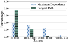
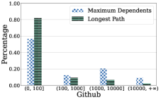
Figure 1: Probability distributions for the maxinum number of dependents and the longest path in the Enron and Github datasets

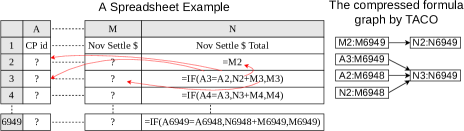
Figure 2: A real spreadsheet with tabular locality [13]

In this paper, we study how we can reduce the execution time for finding dependents and precedents in formula graphs by leveraging predefined patterns found in real spreadsheets. These patterns can be used to compress the formula graph and enable fast look-ups of dependents and precedents directly on the compressed graph. Specifically, our key insight is that cells that are close to each other in the tabular spreadsheet layout often employ similar formula structures, a property we refer to as tabular locality. Fig. 2 shows a column of formulae of a real-world spreadsheet that follows tabular locality. While the formulae in the column N look complicated at first glance, they follow the same pattern starting from N3: the IF formula in each row references the cell of the same row and the row above from column A (e.g., N3 references A3 and A2), the cell to the left (e.g., M3 for N3), and the cell above (e.g., N2 for N3). Tabular locality is prevalent in real-world spreadsheets mainly because users often do not write several distinct formulae by hand, but use spreadsheet features, such as copy-paste and autofill, to generate formulae automatically. Autofill, for instance, allows users to drag a cell to fill adjacent cells by repeating the pattern of the source cell. Users could also programmatically generate a large spreadsheet, which still likely respects tabular locality.

However, leveraging tabular locality to efficiently find dependents and precedents requires addressing several challenges in compressing, querying, and maintaining formula graphs. First, as we show in the experiments (Sec. VI-B), formula references are complex: a formula could include multiple references to different rows or columns (e.g., N3 in Fig. 2 references 4 different cells). Disentangling these multiple references across cells, identifying common patterns across them and compressing these common patterns can be time-consuming. Therefore, the compression algorithm should balance between the quality of the compression (e.g., the number of common patterns detected) and the compression time. While it may be possible to track user actions (e.g., during autofill) to identify and compress formula dependencies directly, this approach does not apply when spreadsheets are shared via files (e.g., xlsx files), losing track of the actions that generated them. It also cannot compress formula dependencies generated programmatically [15, 16]. Furthermore, developing a compressed representation and algorithms for directly querying the compressed graphs to reduce look-up time is also an open challenge Finally, the formula graph needs to be maintained over time, which requires incrementally updating the compressed graph to avoid decompression overhead.

To address these challenges, we present Tabular Locality-based Compression or TACO. In TACO, we leverage four basic patterns that serve as building blocks for other more complicated patterns, and identify one extended pattern based on the analysis of real spreadsheets. We propose a generic framework that decomposes messy formulae and extracts their predefined patterns. This framework is also extensible to support new patterns. We prove that compressing a formula graph using predefined patterns is NP-Hard via a reduction from the rectilinear picture compression problem [17]. We develop a greedy algorithm to efficiently compress formula graphs while maintaining low compression overhead. Further, we design algorithms for finding dependents or precedents directly on the compressed graph, and for maintaining the graph incrementally, and analyze the complexity of each algorithm. Our experiments show that for querying formula graphs, the speedups of TACO over a baseline and a commercial spreadsheet system are up to 34,972$\times$ and 632$\times$, respectively.

While there is a lot of work on graph compression [18], this work does not leverage tabular locality or take into account the spatial nature of spreadsheet ranges. In addition, most of this work does not support directly querying the compressed graph, so these compression algorithms will not be faster than an approach without compression in terms of finding dependents/precedents. Fan et al. [19] propose a method for directly executing reachability and pattern matching queries on a compressed graph, but do not leverage tabular locality nor supporting finding dependents/precedents. TACO is also different from columnar compression [20, 21] because TACO compresses formula dependencies as opposed to columnar data. A recent paper proposes a specialized algorithm for compressing formula graphs [7]. However, this algorithm introduces false positives. In addition, it has a high compression and maintenance time, which we will show in Sec. VI. It turns out that Excel has a capability wherein it identifies identical formulae and stores duplicate formulae as pointers to the first formula [22]. But it does not consider compressing and querying the formula dependencies based on tabular locality.

II Background and Problem

In this section, we present the problem of compressing, querying, and maintaining formula graphs.

II-A Background

Spreadsheets A spreadsheet consists of a set of cells organized in a tabular layout. Each cell is referenced using its column and row index. Columns are identified by letters A, $\cdots$ , Z, AA, $\cdots$, and rows are identified by numbers 1, 2, $\cdots$. For simplicity, for a cell we also use integers $(i,j)$ to represent its position, where $i$ and $j$ are column and row indices, respectively, both starting from 1. A range, akin to a 2D window, is a rectangular region of cells, identified by the top-left (called head) and bottom-right (called tail) cells. For example, the range A1:B2 contains cells A1, A2, B1, B2, with head and tail cells A1 and B2, respectively.

A cell contains a formula or a pure value. A pure value is a constant belonging to a fixed type while a formula is a mathematical expression that takes pure values and/or cell/range references as input. The result of an evaluated formula is an evaluated value. For example, the cells in column A in Fig. 2 include pure values while the cells in column N include formulae. In the rest of the paper, we use “value” to refer to either the pure or evaluated value of a cell. A cell that includes a formula is called a formula cell.

Formula graphs A formula graph is a directed acyclic graph (DAG) that stores the dependencies of each formula referencing other ranges as edges. Specifically, each formula is parsed to get the set of ranges the formula references, with a directed edge added from each referenced range to the formula cell. We call this directed edge a dependency. Given a directed edge $e=(\textit{prec},\textit{dep})$, we call prec the direct precedent of dep or the precedent of the edge $e$. Symmetrically, we call dep the direct dependent of prec or the dependent of $e$.

Fig. 3 shows a spreadsheet with four formulae along with its formula graph. The cells denoted as $?$ are pure values. B1 and B2 have the same formula SUM(A1:A3), so the direct dependents of A1:A3 include B1 and B2. C1 references B1 and B3, so we add two edges. Finally, C2 references B2:B3, which adds an edge with separate vertices although B2:B3 overlaps with the vertices B2 and B3.

The formula graph is used to quickly find the dependents or precedents of an input range. The dependents of an input range are the set of cells that are reachable from the input range in the formula graph. Symmetrically, the precedents are the set of cells that can reach the input range in this formula graph via a directed path. For example, the dependents of A1 are {B1, B2, C1, C2} in Fig. 3. Since a vertex in the graph can be a range, we can build an index (e.g., R-Tree [23]) over the vertices to quickly find the ranges that overlap with an input range. (e.g., find A1:A3 given a cell A1).

One application of the formula graph is to find the dependents when users update the spreadsheet to ensure that users do not see stale or inconsistent results. Specifically, when a cell is updated, the formulae of its dependents will be re-evaluated in sequence to refresh their values. A key prerequisite to updating the formulae is identifying which formulae require recomputation in the first place. If the update is to a formula cell, the formula graph will be modified. The formula graph is also useful for visualizing formula dependencies, which allows users to trace the dependents/precedents of a cell to check the accuracy of formulae or find the sources of errors [12, 9, 8, 15]. In both applications, the performance of querying the formula graph is critical to ensure interactivity.

II-B Compressing, Querying, and Maintaining Formula Graphs

Formula graph problems Finding the dependents and precedents of an input range is often time-consuming due to the size or complexity of the graph. Therefore, we propose compressing formula graphs by leveraging tabular locality to significantly reduce graph size. Directly querying the compressed graph and incremental maintenance can decrease the time taken for finding dependents/precedents and maintaining the graph, respectively, while introducing the modest overhead of building the compressed graph.

Patterns in formula graphs We capture and distill tabular locality in a formula graph via patterns. For a set of edges $A$ of arbitrary size, a pattern is a constant-size (i.e., $O(1)$) representation that can reconstruct $A$ (with size $O(|A|)$). In addition, finding the direct dependents or precedents of an input range in a pattern should also be constant time. Consider Fig. 2 as an example. Each formula cell N$i$ starting from N3 follows the pattern that N$i$ depends on A$i$, A($i$-1), M$i$, and N($i$-1). By storing the relative positions between N$i$ and A$i$, i.e., A$i$ is 13 columns left to N$i$, and the valid range of N$i$, i.e., N3:N6949, we can represent the edges $\textsf{\small A$i$}\rightarrow\textsf{\small N$i$}$ using constant-size information. We can also find dependents/precedents in this compressed edge in constant time. For example, for input range A3:A10, we can use the information of relative positions to find the dependents N3:N10 in constant time. We can represent and query other edges in a similar way. Therefore, leveraging patterns greatly reduces formula graph sizes and consequently reduces the time for finding dependents/precedents.

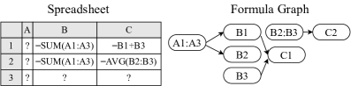
Figure 3: An example spreadsheet and its formula graph

Compressed formula graph representation Given a formula graph $G^{\prime}(E^{\prime},V^{\prime})$, we want to find a lossless compressed graph $G(E,V)$ that preserves the results of finding dependents/precedents. $G$ is generated based on a partition of the edge set $E^{\prime}$ in $G^{\prime}$: $P=\{E_{1}^{\prime},E_{2}^{\prime},\cdots,E_{N}^{\prime}\}$, where $E^{\prime}=\cup_{i=1}^{N}E_{i}^{\prime}$. Each $E_{i}^{\prime}$ must either contain a single edge (i.e., uncompressed), or be a set of edges that follow one of the predefined compression patterns, in which case these edges will be replaced with a compressed edge. We generate a compressed edge $e_{i}=(\textit{prec},\textit{dep},p,\textit{meta})$ for each $E_{i}^{\prime}=\{e_{1}^{i},e_{2}^{i},\cdots,e_{M_{i}}^{i}\}$, where $M_{i}$ is the size of $E_{i}^{\prime}$. The components $e_{i}.\textit{prec}$ and $e_{i}.\textit{dep}$ are the precedent and the dependent of $e_{i}$, computed as $e_{i}.\textit{prec}=\bigoplus_{j=1}^{M_{i}}{e_{j}^{i}.\textit{prec}}$ and $e_{i}.\textit{dep}=\bigoplus_{j=1}^{M_{i}}{e_{j}^{i}.\textit{dep}}$. $\bigoplus$ is the minimal bounding range of the input ranges. For example, $\bigoplus$ merges the ranges A1:A3 and A2:A5 into A1:A5. The component $e_{i}.p$ is the compression pattern while $e_{i}.\textit{meta}$ encodes the underlying pattern information such that meta of an edge $e_{i}$ in $E$ is used to reconstruct the corresponding edges in $E_{i}^{\prime}$. If $E_{i}^{\prime}$ contains a single edge, $e_{i}.p$ is set to Single, which is defined as the pattern for an uncompressed edge. So $E$ in $G$ comprises the edges generated from the partition $P$ and $|E|=N$. The compressed vertex set $V$ is induced from $E$.

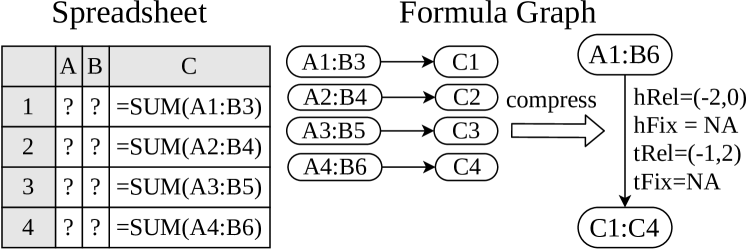
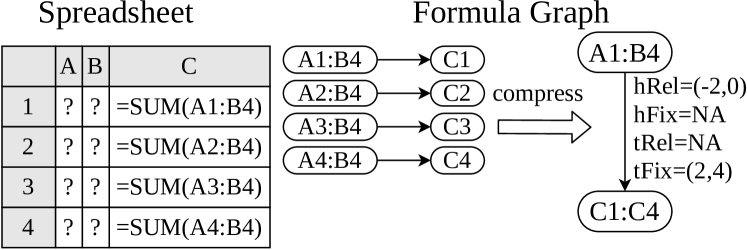
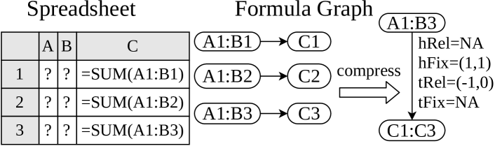
(a) Relative plus Relative (i.e., sliding window) (b) Relative plus Fixed (i.e., shrinking window)

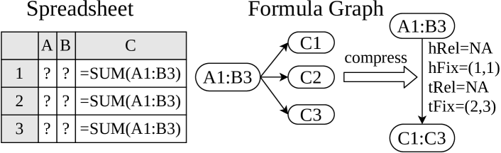
(c) Fixed plus Relative (i.e., expanding window) (d) Fixed plus Fixed (i.e., fixed window)

Figure 4: Examples of four basic patterns of tabular locality

Problem statement Given a set of predefined pattern types, we want to build an equivalent compressed graph $G(E,V)$ of a formula graph $G^{\prime}(E^{\prime},V^{\prime})$ such that the size of $G$ and the time for finding the dependents/precedents of a cell are both significantly smaller compared to $G^{\prime}$, and the time for maintaining $G$ is also smaller than the time for maintaining $G^{\prime}$ with respect to the same updates.

To address this problem, we discuss the basic compression patterns we support (Sec. III). We then present the TACO framework that leverages the basic patterns to compress, query, and maintain a formula graph, and analyze the algorithmic complexity (Sec. IV). Finally, we discuss extending TACO to support new patterns beyond the basic ones (Sec. V).

III Basic Patterns

In this section, we define the basic compression patterns we consider and propose algorithms for using the pattern to build a compressed edge, finding dependents or precedents, and maintaining the edge.

III-A Basic Patterns

The basic patterns consider tabular locality in adjacent formula cells and assume each formula cell references a single range. We can employ the basic patterns multiple times to compress dependencies when formula cells have multiple references, as discussed in Sec. IV-A. We focus on adjacent cells in a column for simplicity; the row-wise case can be derived symmetrically.

Let $A^{\prime}(A^{\prime}\subseteq E^{\prime}$) be a set of dependencies in a column of adjacent formula cells. Our basic patterns capture various relationships between the precedent and dependent of each $e^{\prime}\in A^{\prime}$. Recall that $e^{\prime}.\textit{dep}$ is a formula cell and $e^{\prime}.\textit{prec}$ is a referenced range, represented by the positions of its head and tail cell. In a spreadsheet, there are two types of relationships between the formula cells (i.e., $e^{\prime}.\textit{dep}$) and the head/tail cells in the referenced range (i.e., $e^{\prime}.\textit{prec}$): fixed and relative [24].

The fixed relationship captures the scenario where each dependent $e^{\prime}.\textit{dep}$ references the same head or tail cell of the precedent $e^{\prime}.\textit{prec}$. For example, the formulae in a column all reference a common dollar conversion rate, stored in a fixed location, i.e., a cell. Here, we have a fixed relationship with both the head and the tail cell of the referenced range, which are identical. This is a case of an FF (or Fixed-Fixed) pattern. The referenced head and tail cell for fixed references are denoted hFix and tFix, respectively.

The relative relationship, on the other hand, captures the scenario where each dependent $e^{\prime}.\textit{dep}$ has the same relative position with respect to the head or tail cell of the precedent $e^{\prime}.\textit{prec}$. The relative position with respect to the head and tail cell is denoted hRel and tRel, respectively. One example of a relative position is each formula cell in a column references a cell to its left. Here there is a relative relationship to both the head and tail cell of the referenced range, which are identical. This is a case of an RR (or Relative-Relative) pattern. We use a pair $(p,q)$ to represent the relative position; $p$ denotes the relative column distance and $q$ the relative row distance. Given two cells’ positions $u$ and $v$, we say $u$ is relative to $v$ by $(p,q)$ if $v.i=u.i+p$ and $v.j=u.j+q$.

Combining the two types of relationships (fixed or relative) with the two cells that represent the precedent (head and tail), there are four basic patterns that capture the relationships between dependents and precedents for a column of dependencies. We additionally include a default pattern called Single for an uncompressed edge.

Relative plus Relative (RR) RR is the setting where each $e^{\prime}.\textit{dep}$ has the same relative positions to both head and tail cells of $e^{\prime}.\textit{prec}$. Fig. 4 shows an example. We see that each formula cell in column C is relative to the head cell of its referenced range by $(-2,0)$ (i.e., to the left by two columns) and relative to the tail cell by $(-1,2)$. The metadata meta is ($\textit{hRel}=(-2,0),\textit{hFix}=\textsf{NA},\textit{tRel}=(-1,2),\textit{tFix}=\textsf{NA})$). NA means that this pattern does not include this information (e.g., RR does not reference fixed head or tail cells). So the compressed edge in Fig. 4 is $(\textit{prec}=\textsf{\small A1:B6},\textit{dep}=\textsf{\small C1:C4},p=\textsf{RR},\textit{meta})$, where meta is as defined above.

Relative plus Fixed (RF) RF is the setting where each $e^{\prime}.\textit{dep}$ has the same relative position to the head cell and references a fixed tail cell. Fig. 4 shows an example. Here, each formula in column C is relative to the head cell of its referenced range by $(-2,0)$ and points to a fixed tail cell $\textsf{\small B4}=(2,4)$. The metadata meta equals $(\textit{hRel}=(-2,0),\textit{hFix}=\textsf{NA},\textit{tRel}=\textsf{NA},\textit{tFix}=(2,4))$.

Fixed plus Relative (FR) FR is the dual pattern of RF. So each $e^{\prime}.\textit{dep}$ points to the same head cell and has the same relative position for the tail cell. Fig. 4 shows that the metadata of the compressed edge is $(\textit{hRel}=\textsf{NA},\textit{hFix}=(1,1),\textit{tRel}=(-1,0),\textit{tFix}=\textsf{NA})$.

Fixed plus Fixed (FF) FF is the setting where each $e^{\prime}.\textit{dep}$ references fixed head and tail cells, represented as hFix and tFix, respectively. Fig. 4 shows that each formula cell always points to (A1:B3) and its meta is $(\textit{hRel}=\textsf{NA},\textit{hFix}=(1,1),\textit{tRel}=\textsf{NA},\textit{tFix}=(2,3))$.

Applicability of the basic patterns One major reason why the basic patterns are prevalent in real spreadsheets is that modern spreadsheet systems (e.g., Excel, Google Sheets, and LibreOffice Calc) provide a tool, called autofill, to help users generate a large number of formulae automatically, and the patterns adopted by autofill end up being the basic patterns. Specifically, autofill generates formulae by applying the pattern of one source formula cell to adjacent cells. For the generated formulae, the formula functions (e.g., SUM) are the same as in the source cell, but the references (e.g., A1:B1) are modified based on the following rules: if a reference is prefixed with a dollar sign $, it is a fixed reference; otherwise it is a relative reference. Therefore, if a range $R$ in the source cell does not have $, the generated ranges from $R$ follow the RR pattern. If $R$’s head cell does not have $ but the tail cell does, the generated ranges follow RF. The FR pattern is generated symmetrically. Finally, if $R$’s tail and head cells have $, the generated ranges follow FF. But a formula may mix many ranges and include outliers, which makes extracting basic patterns from these formulae challenging.

While there are other methods for generating formula cells (e.g., programmatically), we believe these methods are still likely to generate the basic patterns since these patterns are the building blocks for many applications. A concrete example that follows RR is in Fig. 2; RR is common in sliding-window-style computation. FR and RF are often employed for cumulative total computation. A real example involves a user sorting transactions by date and using a column of formulae to compute the year-to-date sales amount. FF is also widely used in real applications for referencing fixed ranges for point lookups, e.g., a fixed interest rate or monetary conversion rate in a cell, or range lookups. One example of a FF range lookup is a column of VLOOKUP formulae, each of which looks up a value in the same range. In fact, our experiments in Section VI-B show that leveraging the basic patterns in Section V reduce the number of edges of formula graphs for two real spreadsheet datasets to 5% and 1.9%, respectively, which shows that the basic patterns are prevalent in real spreadsheets.

Discussion on leveraging the basic patterns One natural question is whether existing spreadsheets leverage the basic patterns for compression and querying. Excel does identify the same formulae and stores them efficiently [22], but does not leverage these patterns to accelerate traversing formula graphs, as is verified by our experiments in Sec. VI-E. While it is possible to track autofill expressions to compress formula dependencies, this approach does not apply to spreadsheets generated programatically, and is coupled with a spreadsheet system. To the best of our knowledge, no spreadsheet systems compress and query formula dependencies via tabular locality.

Therefore, we develop general compression algorithms that apply to all spreadsheets. Our algorithms can certainly leverage user actions (e.g., autofill) or cues (e.g., dollar sign) for better compression, but do not rely on it. In addition, we also design novel algorithms for efficiently querying and incrementally maintaining these patterns.

III-B Algorithms for the Basic Patterns

To integrate a pattern into TACO, TACO requires each pattern to implement four key functions, as shown in Fig. 5.

• $\texttt{addDep}(e,e^{\prime})$: add a dependency $e^{\prime}$ to a compressed edge $e$, where $e^{\prime}.\textit{dep}$, the formula cell, is adjacent to $e.\textit{dep}$;

• $\texttt{findDep}(e,r)$: find the dependents of a range of cells $r$ within a compressed edge $e$, where $r$ is contained in $e.\textit{prec}$;

• $\texttt{findPrec}(e,s)$: find the precedents of a range of cells $s$ within a compressed edge $e$, where $s$ is contained in $e.\textit{dep}$;

• $\texttt{removeDep}(e,s)$: remove the dependencies for a range of formula cells $s$ in an edge $e$, where $s$ is contained in $e.\textit{dep}$

The parameter assumptions are guaranteed by TACO framework, discussed in Sec. IV.

1

2 Algorithm addDep($e$, $e^{\prime}$)

3       if $e.p==\textsf{Single}$ then

4             if $\textit{rel}(e)==\textit{rel}(e^{\prime})$ then

5                   return $(e.\textit{prec}\bigoplus e^{\prime}.\textit{prec},e.\textit{dep}\bigoplus e^{\prime}.\textit{dep},\textsf{RR},\textit{rel}(e^{\prime}))$

6                  

7            

8       else if $e.\textit{meta}==\textit{rel}(e^{\prime})$ then

9             return $(e.\textit{prec}\bigoplus e^{\prime}.\textit{prec},e.\textit{dep}\bigoplus e^{\prime}.\textit{dep},\textsf{RR},\textit{meta})$

10            

11       end if

12      return NULL

13      

14

15 Procedure rel($e$)

16       $hRel\leftarrow e.prec.head-e.dep$

17       $tRel\leftarrow e.prec.tail-e.dep$

18       return $(hRel,tRel)$

19

20

21 Algorithm findDep($e,r$)

22       $\textit{prec}_{t}^{d_{h}}\leftarrow(e.\textit{prec}.\textit{tail}.i,\textit{r.{head}}.j)$

23       $d_{h}\leftarrow\textit{prec}_{t}^{d_{h}}-e.\textit{meta}.\textit{tRel}$

24       $\textit{prec}_{h}^{d_{t}}\leftarrow(e.\textit{prec}.\textit{head}.i,\textit{r.{tail}}.j)$

25       $d_{t}\leftarrow\textit{prec}_{h}^{d_{t}}-e.\textit{meta}.\textit{hRel}$

26       return the intersection of $(d_{h},d_{t})$ and $e.\textit{dep}$

27      

28

29

30 Algorithm findPrec($e,r$)

31       $g_{h}\leftarrow r.\textit{head}+e.\textit{meta}.\textit{hRel}$

32       $g_{t}\leftarrow r.\textit{tail}+e.\textit{meta}.\textit{tRel}$

33       return $(g_{h},g_{t})$;

34

35

36 Algorithm removeDep($e,s$)

37       $\textit{newDepSet}\leftarrow$ delete $s$ from $e.\textit{dep}$

38       for $\textit{newDep}\in\textit{newDepSet}$ do

39             $\textit{newPrec}\leftarrow\texttt{findPrec}(e,\textit{newDep})$

40             $p\leftarrow|\textit{newDep}|==1\>?\>\textsf{Single}:\textsf{RR}$

41             add $(\textit{newPrec},\textit{newDep},p,e.\textit{meta})$ to retSet

42            

43       end for

44      return retSet

45

46

Algorithm 1 Algorithms for the RR pattern

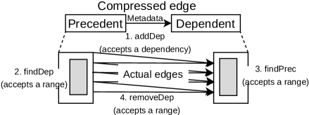
Figure 5: An overview of the four key functions

RR The four key functions for RR are shown in Algorithm 1. Consider $\texttt{addDep}(e,e^{\prime})$, which adds a dependency $e^{\prime}$ to a compressed edge $e$. According to the definition of RR, the dependency $e^{\prime}$ can only be added to $e$ if the relative positions of $e^{\prime}$ equal the relative positions $(\textit{hRel},\textit{tRel})$ in $e.meta$. We define $\textit{rel}(e^{\prime})$ as the procedure to compute the relative positions of $e^{\prime}.\textit{dep}$ with respect to the head and tail cell of $e^{\prime}.\textit{prec}$, respectively (i.e., line 9-12 in Algorithm 1). For example, if $e^{\prime}=\textsf{\small A5:B7}\rightarrow\textsf{\small C5}$, the relative positions are $\textit{hRel}=\textsf{\small A5}-\textsf{\small C5}=(-2,0)$ and $\textit{tRel}=\textsf{\small B7}-\textsf{\small C5}=(-1,2)$. This dependency can be added to the compressed edge $e$ in Fig. 4 because $e.meta.\textit{hRel}$ and $e.meta.\textit{tRel}$ equal hRel and tRel, respectively. Therefore, we create a new compressed edge, where $\textit{prec}=e.\textit{prec}\bigoplus e^{\prime}.\textit{prec}$, $\textit{dep}=e.\textit{dep}\bigoplus e^{\prime}.\textit{dep}$, and $meta=e.meta$. If $e$ is an uncompressed edge (a single dependency), we compare $\textit{rel}(e^{\prime})$ and $\textit{rel}(e)$ to check whether the two edges can be compressed using the RR pattern.

Next, consider $\texttt{findDep}(e,r)$, which finds the dependents (denoted as a range $d$) of a range of cells $r$ that are contained in $e.\textit{prec}$. To determine $d$, we need to find its head cell $d_{h}$ and tail cell $d_{t}$. Since the precedent of each cell in $d$ forms a sliding window on $e.\textit{prec}$ as shown in Fig. 7, the intuition for computing $d_{h}$ is that the top row of $r$ must intersect with the bottom row of $d_{h}$’s precedent. Similarly, the bottom row of $r$ must intersect with the top row of $d_{t}$’s precedent. So we “back calculate” $d_{h}$ and $d_{t}$ based on $r$. Specifically, we use the following invariant to compute $d_{h}$,

$$d_{h}+\textit{tRel}=\textit{prec}_{t}^{d_{h}}$$

where $\textit{prec}_{t}^{d_{h}}$ is $d_{h}$’s precedent’s tail cell and tRel is the relative position of $d_{h}$ with respect to $\textit{prec}_{t}^{d_{h}}$ as shown in Fig. 7. Since tRel is known, the remaining task is to compute $\textit{prec}_{t}^{d_{h}}$. We know that $\textit{prec}_{t}^{d_{h}}$ is in the bottom row of $d_{h}$’s precedent since it is a tail cell and that the bottom row of $d_{h}$’s precedent intersects the top row of $r$. So $\textit{prec}_{t}^{d_{h}}$ is in the top row of $r$ and its row index is the row index of $r$’s head cell (i.e., $r.\textit{head}.j$). Since $\textit{prec}_{t}^{d_{h}}$ is a tail cell, it is in the right-most column of $e.\textit{prec}$. So its column index is $e.\textit{prec}.\textit{tail}.i$.

Figure 6: An example of $\texttt{findDep}(e,r)$ for RR Figure 7: An example of $\texttt{findDep}(e,r)$ for RF

Finding the tail cell $d_{t}$ adopts a dual procedure. Based on the invariant $d_{t}+\textit{hRel}=\textit{prec}_{h}^{d_{t}}$, we need to find $d_{t}$’s precedent’s head cell $\textit{prec}_{h}^{d_{t}}$. As shown in Fig. 7, $\textit{prec}_{h}^{d_{t}}$ should be in the last row of $r$ and in the left-most column of $e.\textit{prec}$. Therefore, we have $\textit{prec}_{h}^{d_{t}}.i=e.\textit{prec}.\textit{head}.i$ and $\textit{prec}_{h}^{d_{t}}.j=r.\textit{tail}.j$. We note this procedure can output a range $d$ that is beyond $e.\textit{dep}$. In this case, we take the intersection between $d$ and $e.\textit{dep}$ to return a valid range.

The third function, $\texttt{findPrec}(e,s)$ finds the precedents (denoted as a range $g$) for a range of cells $s$ contained in $e.\textit{dep}$. By the definition of RR, the precedents of the cells in $s$ form “sliding windows” on $e.\textit{prec}$ as we move from $s.\textit{head}$ to $s.\textit{tail}$; $g$ is simply the union of the precedents of all cells in $s$. So $g.\textit{head}$ is the head cell of $s.\textit{head}$’s precedent and $g.\textit{tail}$ is the tail cell of $s.\textit{tail}$’s precedent. We have $g.\textit{head}=s.\textit{head}+\textit{hRel}$ and $g.\textit{tail}=s.\textit{tail}+\textit{tRel}$.

Finally, consider $\texttt{removeDep}(e,s)$, which removes the dependencies for a range of formula cells $s$ in $e.\textit{dep}$. We first subtract $s$ from $e.\textit{dep}$, after which we are left with a range or a union of two ranges. For example, if we remove C2 from C1:C4, the remainder is composed of two ranges: C1 and C3:C4. For each range newDep in the remaining dependents, we generate its corresponding precedent newPrec using $\texttt{findPrec}(e,\textit{newDep})$.

RF, FR, FF We now discuss the key functions for RF. The function $\texttt{addDep}(e,e^{\prime})$ for the RF pattern has similar logic to the one for RR and is different only in the compression condition. By definition of RF, we first compute the relative position between $e^{\prime}.\textit{dep}$ and the head cell of $e^{\prime}.\textit{prec}$ (denoted hRel) and check whether hRel and $e.meta.\textit{hRel}$ are the same. If so, we additionally check whether the tail cell of $e^{\prime}.\textit{prec}$ is the same as $e.meta.\textit{tFix}$.

$\texttt{findDep}(e,r)$ finds the range of dependents $d$ for a range of cells $r$ contained in $e.\textit{prec}$. Similar to RR, we need to find $d$’s head cell $d_{h}$ and tail cell $d_{t}$. To compute $d_{h}$, we use the intuition shown in Fig. 7: the precedent of $e.\textit{dep}.\textit{head}$ equals $e.\textit{prec}$ and the precedent of each cell in $e.\textit{dep}$ shrinks when we move from $e.\textit{dep}$’s head to its tail cell. That is, $e.\textit{dep}.\textit{head}$ references the entire range of $e.\textit{prec}$ and is the dependent of any $r$ contained in $e.\textit{prec}$. So $e.\textit{dep}.\textit{head}$ equals $d_{h}$.

To compute $d_{t}$, we use the observation that the precedent of each cell in $e.\textit{dep}$ shrinks as we move from $d_{h}$ to $d_{t}$ such that the bottom row of $r$ should intersect with the top row of the precedent of $d_{t}$. Therefore, to compute $d_{t}$, we leverage the invariant $d_{t}+\textit{hRel}=\textit{prec}_{h}^{d_{t}}$, where $\textit{prec}_{h}^{d_{t}}$ is the head cell of $d_{t}$’s precedent. Since hRel is known, we need to compute $\textit{prec}_{h}^{d_{t}}$. As Fig. 7 shows, since $\textit{prec}_{h}^{d_{t}}$ is in the bottom row of $r$, its row index is $r.\textit{tail}.j$ and since $\textit{prec}_{h}^{d_{t}}$ is a head cell, its column index is $e.\textit{prec}.\textit{head}.i$.

Consider $\texttt{findPrec}(e,s)$, which finds the precedents (denoted as a range $g$) of $s$ contained in $e.\textit{dep}$. Our observation is that the precedent of $s.\textit{head}$ contains all of the precedents of other cells in $s$ since the precedent of each cell in $e.\textit{dep}$ is shrinking as we move from $s.\textit{head}$ to $s.\textit{tail}$. Therefore, $g$ is the precedent of $s.\textit{head}$, and is computed as $g.\textit{head}=s.\textit{head}+\textit{hRel}$ and $g.\textit{tail}=\textit{tFix}$. The function $\texttt{removeDep}(e,s)$ for RF follows the same logic as RR. We first remove $s$ from $e.\textit{dep}$ to return one or two ranges. For each returned range newDep, we generate their corresponding precedent newPrec using $\texttt{findPrec}(e,\textit{newDep})$ of RF.

FR is a dual pattern of RF, so its algorithms can be easily derived from the algorithms above. FF’s algorithms can also be derived from FR and RF. We omit these algorithms due to space limits.

Algorithmic complexity All algorithms for the basic patterns are $O(1)$, independent of the number of edges compressed.

IV TACO Framework

We now introduce the TACO framework, which includes four generic and extensible algorithms for efficiently compressing, querying, and modifying formula graphs. These algorithms are extensible since they only utilize the four key functions per pattern as shown in Section III-B and any pattern can be integrated into the TACO framework if they implement these functions. In this section, we first introduce these algorithms and analyze their complexity (Sec. IV-A-IV-C). Then, we compare the complexity of TACO against an approach that does not compress the formula graph (Sec. IV-D). We assume the formula graphs in both approaches are implemented via an adjacency list and we build an R-Tree index on the vertices to quickly find the overlapping vertices for an input range. The complexity of operations on an R-Tree varies based on the design choices. Our analysis assumes the complexity for searching, inserting, and deleting one range is $O(N)$, $O(\log N)$, and $O(\log N)$, respectively, where $N$ is the number of ranges stored in the R-Tree.

1

2Algorithm addDep($G(E,V)$, $e^{\prime}$)

3       $\textit{isCompressed}\leftarrow$ false

4      

5      $\textit{pSet}\leftarrow$ pre-defined patterns

6       $\textit{eSet}\leftarrow$ find all $e\in E$ whose $e.\textit{dep}$ is adjacent to

7                  $e^{\prime}.\textit{dep}$ on column or row axis

8      

9      for $\textit{candE}\in\textit{eSet}$ do

10             $\textit{edgePairs}\leftarrow$ genCompEdges(candE, $e^{\prime}$, pSet)

11             $\textit{edgePairSet}.\texttt{add}(\textit{edgePairs})$

12            

13       end for

14      

15      if edgePairSet is not empty then

16             $\textit{edgePair}\leftarrow$ sort edgePairSet by heuristics and

17                              take the first

18             maintain $G$ using edgePair

19             $\textit{isCompressed}\leftarrow$ true

20             break

21            

22       end if

23      if isCompressed is false then

24             insert $e^{\prime}$ into $G$

25            

26      

27

28

29 Procedure genCompEdges(candE, $e^{\prime}$, pSet)

30       if $\textit{candE}.p==\textsf{Single}$ then

31             for $p\in\textit{pSet}$ do

32                   $\textit{pair}\leftarrow(p.\texttt{addDep}(\textit{candE},e^{\prime}),\textit{candE})$

33                   $\textit{edgePairs}.\texttt{addIfValid}(\textit{pair})$

34                  

35             end for

36            

37       else

38             $\textit{pair}\leftarrow(\textit{candE}.p.\texttt{addDep}(\textit{candE},e^{\prime}),\textit{candE})$

39             $\textit{edgePairs}.\texttt{addIfValid}(\textit{pair})$

40            

41       end if

42      return edgePairs

43      

44

Algorithm 2 Compressing a dependency $e^{\prime}$ into $G(E,V)$

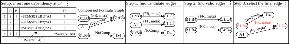
Figure 8: An example of compressing one dependency inserted at C4

IV-A Compressing a Formula Graph

We formalize the problem of minimizing the number of edges of the compressed formula graph based on the predefined basic patterns and present our compression algorithm.

IV-A1 Problem formalization

Using the definition of the compressed graph $G$, the problem of minimizing the number of edges in $G$ is equivalent to the problem of finding a partition $P=\{E_{1}^{\prime},E_{2}^{\prime},\cdots,E_{N}^{\prime}\}$ of the uncompressed edge set $E^{\prime}$ such that $N$ is minimum, and each $E_{i}^{\prime}$ is compressed by a single pattern or only includes one uncompressed edge. The optimization problem, which we call Compressed Edge Minimization (or CEM for short), is defined as follows:

$$\underset{P=\{E_{1}^{\prime},\cdots,E_{N}^{\prime}\}}{\text{minimize}} N$$

where $$E_{i}^{\prime}\text{ is compressed by a pattern or is}$$

$$\text{an uncompressed edge,}\forall i\in 1\ldots N$$

$$\,\cup_{i}E_{i}^{\prime}=E^{\prime}$$

We now show CEM is NP-Hard even when we only consider each basic pattern.

Theorem 1 (CEM Hardness).

Compressing the graph $G^{\prime}$ into $G$ while minimizing the number of edges of $G$ is NP-Hard, even when restricted to each basic pattern.

Proof.

(Sketch) We reduce the rectilinear picture compression (RPC for short) problem, which is known to be NP-Hard [17], to CEM. The input to RPC is a $m\times n$ matrix of 0’s and 1’s, with the goal to find the minimal number of rectangles that precisely cover the 1’s. We reduce RPC to CEM by mapping the input matrix to a spreadsheet range $R$: for each value at column $i$ and row $j$ in the matrix, if the value is 1, we place a formula at $(i,j)$ in $R$; otherwise, we place a pure value at $(i,j)$ in $R$. If the dependencies of any range of formulae in $R$ can be compressed into a single edge by a pattern $p$, then the RPC problem is equivalent to minimizing the number of edges of the compressed graph $G$ for $R$ if we only consider the pattern $p$.

Therefore, we need to construct a range $R$ for each pattern $p$ such that the dependencies of any range of formulae in $R$ can be compressed into a single edge by $p$. For FF, we let all of the formulae in $R$ reference the same fixed range outside $R$ to meet the above condition. Similarly, for RR, we let each formula in $R$ reference the cell to its left. For RF, we first construct another range $R^{\prime}$ that can be compressed into a single edge by RF and has the same shape as $R$. Note that in $R^{\prime}$, the dependencies of any range of formulae can also be compressed into a single edge by RF. Afterwards, we generate $R$ by copying the formula at $(i,j)$ in $R^{\prime}$ to $(i,j)$ in $R$ if the cell $(i,j)$ in $R$ is a formula cell. This way, we construct a range $R$ where the dependencies of any range of formulae in $R$ can be compressed into a single edge by RF. The case for FR is done symmetrically. ∎

CEM is also trivially NP-Complete since verifying that a partition using FF is correct is in PTIME. We tested the algorithm that enumerates all possible partitions and found it cannot finish within 30 mins for a spreadsheet with 96 edges because the number of possible partitions is a Bell number [25]. To reduce the compression overhead, we propose a greedy compression algorithm.

IV-A2 Greedy compression algorithm

Our algorithm compresses a list of dependencies between formula cells and their referenced ranges by repeatedly inserting each dependency into the compressed graph and determining the partitions as well as the corresponding compression patterns. Observing that pre-defined patterns compress the dependencies in adjacent formula cells, we use this constraint to quickly find the candidate edges that one inserted dependency can be compressed into. If there are multiple candidate edges, we leverage several heuristics based on our analysis of real-world spreadsheets to decide the edge that can best reduce the graph size (e.g., by leveraging the dollar sign cues in the formula expression if available).

Algorithm 2 shows our approach for compressing one dependency $e^{\prime}=(\textit{prec},\textit{dep})$ into a compressed formula graph $G$. We use the example in Fig. 8 to explain compressing $e^{\prime}$ into $G$. The setup of Fig. 8 (the left pane) shows each formula cell in column C referencing two ranges. The references to column B follow FR and the references to column A follow FF. In addition, we have an uncompressed edge of D4 referencing B1:B4. Our example assumes that a formula SUM($B$1:B4) is inserted at C4 (i.e., $e^{\prime}=(\textsf{\small B1:B4},\textsf{\small C4})$).

Find candidate edges: The first step is to quickly find candidate edges that the dependency $e^{\prime}$ can be compressed into. Specifically, an edge $e$ is a candidate if $e.\textit{dep}$ is adjacent to $e^{\prime}.\textit{dep}$ along the row or column axis. Step 1 in Fig. 8 shows that all three edges meet this condition because $e^{\prime}.\textit{dep}=\textsf{\small C4}$ is adjacent to both C1:C3 and D4. To find these edges, we first shift $e^{\prime}.\textit{dep}$ by one cell in all four directions (i.e., up/down/left/right) and use the index on the vertices (e.g., an R-Tree [23]) to quickly find ranges that overlap with the shifted $e^{\prime}.\textit{dep}$. Then, for each overlapping range (e.g., D4), we find its precedent (e.g., B1:B4) and add this edge (e.g., $\textsf{\small B1:B4}\rightarrow\textsf{\small D4}$) into the candidate edge set.

Find valid candidates: Next, we check whether $e^{\prime}$ can be compressed into each candidate edge using $\texttt{addDep}(e,e^{\prime})$ from Sec. III to find the valid compressed edges (i.e., genCompEdges in Algorithm 2). We consider two cases. First, if the candidate edge candE is not compressed, we check whether $e^{\prime}$ and candE can be compressed into a new edge newEdge using the predefined patterns. If so, we store newEdge as a valid candidate edge (i.e., addIfValid in Algorithem 2). If, instead, candE is a compressed edge, we check whether $e^{\prime}$ can be compressed into candE and if so, we generate a valid edge. Step 2 in Fig. 8 shows two valid compressed edges because the edge $\textsf{\small B1:B4}\rightarrow\textsf{\small C4}$ can be compressed into $\textsf{\small B1:B3}\rightarrow\textsf{\small C1:C3}$ or $\textsf{\small B1:B4}\rightarrow\textsf{\small D4}$.

Select the final edge: The final step is to select the final edge from the valid ones. The selection is based on the following heuristics, in order. First, we prioritize column-wise compression over row-wise compression. If this heuristic does not return a single edge, we further compare the priority of each remaining edge’s pattern. If one pattern $p_{a}$ is a special case of another pattern $p_{b}$, then we choose $p_{a}$ over $p_{b}$ because we expect the special pattern $p_{a}$ to be more efficient. In Sec. V, we will describe one such special pattern of RR. Otherwise, we leverage the dollar sign ($) information, if available, sometimes specified as part of the formula strings. For example, for the formula string SUM($B$1:B4) at C4, we will prioritize compressing its dependency $\textsf{\small B1:B4}\rightarrow\textsf{\small C4}$ using FR over other patterns because the head cell $B$1 in SUM($B$1:B4) has dollar sign annotations, but its tail cell does not, which indicates that SUM($B$1:B4) follows the FR pattern if it is generated via autofill. For our example in Fig. 8, we choose the compressed edge ($\textsf{\small B1:B4}\rightarrow\textsf{\small C1:C4}$) over ($\textsf{\small B1:B4}\rightarrow\textsf{\small C4:D4}$) because the former one uses column-wise compression. Finally, we delete the old edge and insert the newly compressed edge.

Algorithmic complexity Our analysis assumes the inserted dependencies have no duplicates, so its size is $|E^{\prime}|$, the number of uncompressed edges. For each inserted dependency, we leverage the R-Tree to find the candidate edges, taking $O(|V|)$ operations, where $|V|$ is the number of vertices in the compressed formula graph $G$. The number of the candidate edges is $O(|E|)$. For these candidate edges, it takes $O(|E|)$ operations to find the valid compressed edges and the final edge that the input dependency is compressed into. In addition, we need to maintain the R-Tree by removing the old and inserting the new vertices, which takes $O(\log|V|)$ operations. In total, the complexity of inserting $|E^{\prime}|$ dependencies is $O(|E^{\prime}|\times(|V|+|E|+\log|V|))$ = $O(|E^{\prime}|\times|E|)$ since each vertex is connected to at least one edge.

1

2initiate queue as a queue containing only $r$

3 initiate result as an empty set and an R-Tree for it

4 while queue is not empty do

5       $\textit{precToVisit}\leftarrow$ remove the first element in queue

6       $\textit{precs}\leftarrow$ find vertices that overlap with

7                  precToVisit via the R-Tree on V

8       for $\textit{prec}\in\textit{precs}$ do

9             $\textit{edges}\leftarrow$ $\{e:e\in E$ and $e.\textit{prec}=\textit{prec}\}$

10             for $e\in\textit{edges}$ do

11                   $\textit{dep}\leftarrow e.p.\texttt{findDep}(e,\textit{precToVisit})$

12                   $\textit{newDepSet}\leftarrow$ Find the subset of dep not

13                          contained in result via the R-Tree on result

14                   for $\textit{newDep}\in\textit{newDepSet}$ do

15                         add newDep to result and its R-Tree

16                         add newDep to queue

17                        

18                   end for

19                  

20             end for

21            

22       end for

23      

24 end while

25return result

Algorithm 3 Find dependents of a column/row of cells $r$ in $G(E,V)$

IV-B Querying a Formula Graph

We now discuss finding the dependents or precedents of a column/row of cells $r$ in $G$ using the key functions from Sec. III. Since finding dependents is the dual problem of finding precedents, we focus on the former. We apply Breadth-First-Search (BFS), but with three major differences. First, when we find the direct dependents of $r$, we need to consider all of the vertices in $G$ that overlap with $r$. Second, since an edge $e$ in $G$ can be a compressed edge, finding the direct dependents of $r$ in $e$ may not be the full $e.\textit{dep}$, but a subset instead. So we need to find the real dependents within $e.\textit{dep}$. Third, for a “real” dependent, which will in turn serve as a precedent for subsequent searches, we need to add the subset of this dependent that has not yet been visited during BFS. We illustrate the three modifications below.

Algorithm 3 shows the modified BFS algorithm: it takes a column or row of cells $r$ as input and returns the set of ranges that depend on $r$. We explain this algorithm using the compressed graph in Step 3 of Fig. 8. Our example involves finding the dependents of B2. Our algorithm uses a queue to store the ranges to be visited in the future and a set result to store the ranges that depend on $r$ and have been visited. An additional R-Tree is also built for result. For each range precToVisit in this queue, we find its direct dependents. As mentioned earlier, we need to consider the ranges that overlap with precToVisit (i.e., B1:B4 for B2). Next, we find the direct dependents of each overlapping range and the corresponding edges (i.e., $\textsf{\small B1:B4}\rightarrow\textsf{\small C1:C4}$ and $\textsf{\small B1:B4}\rightarrow\textsf{\small D4}$). Since some of these edges can be compressed, for a compressed edge $e$ we need to find the real direct dependent within $e.\textit{dep}$ for precToVisit, which is done by the key function $\texttt{findDep}(e,\textit{precToVisit})$. For the example of the input B2, we return C2:C4 for the edge $\textsf{\small B1:B4}\rightarrow\textsf{\small C1:C4}$ since C1 does not depend on B2. Finally, we find the subset of the real dependent that has not yet been visited via the R-Tree on the result set, and add the subset to the queue, the set result, and the R-Tree on result. We repeat the process until the queue is empty. For the example of the dependent C2:C4, if we have visited C2:C3, we will only store C4 in the queue and result.

Algorithmic complexity To analyze the complexity of Algorithm 3, we consider two cases: 1) Algorithm 3 accesses each edge in $G$ at most once; 2) otherwise. For the first case, each vertex in $G$ will serve as the precedent at most once when we find direct dependents (i.e., the inner part of the first for loop in Algorithm 3). So it will only repeat $O(|V|)$ times. To find a precedent (i.e., prec in the first for loop in Algorithm 3), we need to search the R-Tree, taking $O(|V|)$. To find the real direct dependents for a precedent using findDep, we need to spend $O(dep\_num)$ operations, where $dep\_num$ is the number of direct dependents of a precedent and findDep takes a constant time. For each real direct dependent, we need to additionally find the subset that is not contained in result using the R-Tree on result, taking $O(\text{size of {result}})$. Since each range in result will be a precedent, the size result is $O(|V|)$. In addition, the total cost for maintaining the R-Tree on result is $O(|V|\times\log|V|)$ since the size of result is $O(|V|)$. To sum up, the complexity here is $O(|V|)\times(O(|V|+O(dep\_num)\times O(|V|))+O(|V|\times\log|V|)=O(|V|^{2}+|E|\times|V|)$.

For the second case, the first while loop in Algorithm 3 runs $O|V^{\prime}|$ times, where $|V^{\prime}|$ is the number of vertices in the uncompressed graph. This is because the size of result is $O(|V^{\prime}|)$, so the total number of ranges inserted into the queue is also $O(|V^{\prime}|)$. For each range precToVisit in the queue, we check $O(|E|)$ edges in $G$. For each edge, we find the real dependent using $O(1)$ and take $O(|V^{\prime}|)$ operations to find the subset of the real dependent that is not contained in result. The total cost for maintaining the R-Tree on result is $O(|V^{\prime}|\times\log|V^{\prime}|)$. So the complexity is $O(|V^{\prime}|)\times(O(|V|)+O(|E|\times|V^{\prime}|))+O(|V^{\prime}|\times\log|V^{\prime}|$ = $O(|V^{\prime}|^{2}\times|E|)$.

IV-C Maintaining a Formula Graph

We now discuss maintaining the formula graph when users insert, clear, or update formula cells. We process inserts using Algorithm 2 . Since an update can be modeled as a clearing operation plus an insert, we focus on clearing formula cells.

The idea of clearing a column/row of formula cells $s$ is to delete $s$ from the edges whose dependents (i.e., formula cells) overlap with $s$ using $\texttt{removeDep}(e,s)$ from Sec. III. First, we find the relevant edges relEdges whose dependents overlap with $s$. Second, for each $e\in\textit{relEdges}$, we generate new edges newESet after clearing $s$ for $e$, which is done by $\texttt{removeDep}(e,s)$. Finally, we maintain the graph by deleting the old edge relEdges and inserting the new edges newESet.

Algorithmic complexity For this algorithm, the size of the relevant edges whose dependents overlap with s is $O(|E|)$ and searching the R-tree takes $O|V|)$, so the cost for finding relevant edges is $O(|E|)$. From each relevant edge, clearing s and maintaining the graph is $O(1)$ while maintaining the R-tree takes $O(\log|V|)$ time. In total, the complexity for removing s is $O(|E|\log|V|)$.

	TACO	NoComp
Building	$O(|E^{\prime}|\times|E|)$	$O(|E^{\prime}|\times\log|V^{\prime}|)$
Querying	Case 1: $O(|V|^{2}+|E|\times|V|)$ Case 2: $O(|V^{\prime}|^{2}\times|E|)$	$O(|V^{\prime}|^{2}+|E^{\prime}|)$
Maintaining	$O(|E|\log|V|)$	$O(|E^{\prime}|\log|V^{\prime}|)$

TABLE I: Complexity comparison between TACO and NoComp

IV-D Complexity Comparison with a No Compression Approach

We now compare the complexity of TACO with an approach that does not compress the formula graph, called NoComp. Table I summarizes the results.

NoComp builds the uncompressed formula graph $G^{\prime}$ by inserting a list of dependencies into $G^{\prime}$. For each dependency, we need to insert its precedent and dependent into an R-Tree, taking $O(\log|V^{\prime}|)$ operations, and insert the dependency into the adjacency list, taking $O(1)$. In total, the complexity of inserting $|E^{\prime}|$ dependencies is $O(|E^{\prime}|\times\log|V^{\prime}|)$. TACO can be more expensive than NoComp for building the formula graph because it needs to search the R-Tree and find the edge that an inserted dependency can be compressed into.

Next, we analyze the complexity of finding dependents of an input range $r$ via a modified BFS. During BFS, when we find the direct dependents of an input range $r$, we need to consider all of the vertices in $G^{\prime}$ that overlap with $r$ (i.e., via an R-Tree search). Similar to conventional BFS, it recursively finds dependents starting from the input range $r$. Each vertex in $G^{\prime}$ may serve as a precedent when we find direct dependents of a precedent (i.e., $O(|V^{\prime}|)$ times), while the cost for finding one precedent via the R-Tree is $O(|V^{\prime}|)$. Finding direct dependents of one precedent is $O(dep\_num)$, where $dep\_num$ is the number of the direct dependents. The overall complexity for finding dependents is $O(|V|^{\prime})\times(O(|V^{\prime}|)+O(dep\_num))=O(|V^{\prime}|^{2}+|E^{\prime}|)$.

We see thatTACO is more efficient than NoComp if the querying algorithm of TACO accesses each edge in the compressed graph $G$ at most once (i.e., Case 1 in Table I). For Case 2, TACO can be potentially more expensive than NoComp in theory. To understand the performance of Case 2, we analyze real spreadsheets to find when this case will happen and become the performance bottleneck, and adopt an extended pattern to reduce the cost for this case in Sec. V. In practice, we find the average number of accesses for an edge during BFS is relatively low. For the tests for finding dependents in Sec. VI, the average number of edge accesses during BFS is no larger than 7 for 98% of the tests. In addition, our experiments in Sec. VI show that TACO is much more efficient than NoComp on real spreadsheets.

Finally, clearing a column/row of formula cells s requires searching the R-tree to find relevant edges (i.e., $O(|E^{\prime}|)$). Then, we will delete each relevant edge and update the R-tree (i.e., $O(\log|V^{\prime}|)$). In total, the complexity is $O(|E^{\prime}|\log|V^{\prime}|)$. As shown in Table I, TACO is more efficient here.

V Extension and Limitations

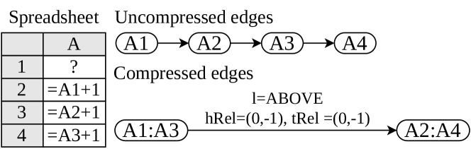
Figure 9: One example of RR-Chain

Supporting a new pattern: RR-Chain As shown in Sec. IV, our algorithm for finding dependents or precedents may be slow if an edge is repeatedly accessed multiple times. By examining real spreadsheets, we find one pattern that leads to these cases and becomes a performance bottleneck for TACO. In this section, we discuss supporting this pattern to further accelerate TACO. Our discussion focuses on a column of cells and finding dependents as before; the other cases can be derived symmetrically.

Consider a column of formula cells that form a chain of dependencies, where each formula cell references its adjacent formula cell above or below. We will compress these dependencies using RR because each formula cell has the same relative position with respect to its referenced range. Consider the example in Fig. 9, where each formula cell starting from A2 increments the value of the above formula cell by one. To find the dependents of A1, we first find its overlapping vertex A1:A3 and then compute its real direct dependent: A2. Afterwards, the compressed edge is repeatedly accessed until we reach the end of this chain, which introduces high searching overhead.

To solve this problem, we introduce a new pattern RR-Chain as a special case of RR. RR-Chain’s meta additionally includes a variable $l$ to indicate the direction of a formula cell referencing its adjacent cell. For example, $l$ is ABOVE in Fig. 9 because each formula cell references its adjacent cell above. Our discussion focuses on $l=\textsf{\small ABOVE}$; the case for $l=\textsf{\small BELOW}$ can be easily derived. To compress a dependency $e^{\prime}$ into $e$ for RR-Chain, we first check the condition of RR, and then further check whether $e^{\prime}.\textit{prec}$ is above $e^{\prime}.\textit{dep}$ and if they are adjacent. To find dependents of a range $r$, we return a range $d$ between $r.\textit{head}$’s direct dependent and the tail cell of $e.\textit{dep}$. Consider finding dependents of A2 in Fig. 9. We return the range between A3 (i.e., A2’s direct dependent) and the tail cell of $e.\textit{dep}$ (i.e., A4). Finally, clearing formula cells in $e.\textit{dep}$ follows the same logic as RR and is omitted.

Limitations One limitation of the patterns in TACO is that they focus on adjacent formula cells. So, they only represent a subset of tabular locality in spreadsheets. It is possible to extend these patterns and exploit other patterns to further reduce the sizes of formula graphs. For example, one extended pattern derived from RR could be that the referenced ranges in the formula cells of every other row follow the RR pattern (denoted as RR-GapOne). We have tested its prevalence and found it is much less prevalent than its RR counterpart. Specifically, RR-GapOne reduces the number of edges by 195k and 275k for Enron and Github datasets, respectively, while the number of edged reduced by RR is 17.4M and 141.9M, respectively (Details in Section VI-B). Also, it is possible to exploit other information, such as a column of formulae having the same functions, to better compress formula graphs. Fully exploiting these patterns and information is left to future work.

VI Experiments

	Enron		Github
	Vertices	Edges	Vertices	Edges
NoComp	18.6M	23.7M	165.8M	179.8M
TACO-InRow	7.7M (41.2%)	12.5M (52.8%)	55.2M (33.3%)	55.2M (30.7%)
TACO-Full	1.2M (6.3%)	1.2M (5.0%)	4.2M (2.5%)	3.5M (1.9%)

TABLE II: Graph sizes after TACO compression (lower is better)

		Max	75th per.	Median	Mean
Enron	TACO-InRow	142,396	18,196	12,489	18,876
	TACO-Full	700,155	37,286	18,380	37,963
Github	TACO-InRow	1,693,698	42,728	19,704	45,303
	TACO-Full	3,139,011	75,553	31,608	78,633

TABLE III: The num. of edges reduced by TACO (higher is better)

Our experiments address the following research questions:

• How much do TACO’s predefined patterns reduce formula graph sizes for real-world spreadsheets? (Sec. VI-B)

• How much time does TACO take to build, query, and maintain a formula graph compared to NoComp, an approach specialized for formula graph compression, and a baseline that implements the formula graph in a graph database? (Sec. VI-C and Sec. VI-D)

• How much faster does TACO query a formula graph compared to a commercial spreadsheet system and a baseline from an open-source spreadsheet system? (Sec. VI-E)

VI-A Prototype, Benchmark, and Configurations

Prototype TACO is implemented as a Java library. It takes an xls or xlsx file as input, leverages the POI library [16] to parse it, and builds a compressed formula graph for the parsed dependencies.The compressed formula graph is implemented using an adjacency list. We build an R-Tree [23] on the vertices of the formula graph to quickly find vertices that overlap with a given range. TACO provides interfaces of finding dependents or precedents of a range, and adding or deleting a dependency. TACO is integrated into DataSpread [26, 27, 28], an open-source spreadsheet system. DataSpread returns control to users after it has identified all of the dependents of an update and hides them; so finding dependents of an update is the bottleneck for returning control to users. In DataSpread, a formula graph is used to find the dependents of an update and TACO acts as a drop-in replacement for this formula graph. TACO can also be integrated into other spreadsheet systems, such as LibreCalc or MS Excel, to accelerate updating spreadsheets since these spreadsheets system similarly adopt formula graphs to track formula dependencies [6, 5]. In addition, TACO can be used by third-party tools to analyze and trace formula dependencies. We have additionally implemented a plug-in using TACO to help users efficiently trace formula dependencies in Excel [29].

Benchmark Our tests are based on two real-world spreadsheet datasets. The first one is the Enron dataset [13] with 17K xls files. We focus on the large spreadsheets (i.e., with no less than 10K dependencies) that do not cause exceptions (e.g., those requiring passwords), and are left with 593 xls files. Since the Enron dataset includes only xls files, we further crawl 7.8K xlsx files from Github that are larger than 10 KB. We focus on large spreadsheets and skip the erroneous ones, and get 2,238 xlsx files. In total, we test 2,831 files.

		Min	25th per.	Median	Mean
Enron	TACO-InRow	0.0042%	6.32%	39.81%	42.27%
	TACO-Full	0.0042%	0.47%	1.93%	7.37%
Github	TACO-InRow	0.0005%	0.10%	17.45%	36.48%
	TACO-Full	0.0005%	0.03%	0.19%	3.44%

TABLE IV: Remaining edges after compression (lower is better)

Pattern	Enron Total	Enron Max	Github Total	Github Max
RR	17,412,246	525,026	141,876,182	2,094,936
RF	1,880	1,413	13,361	9,999
FR	150,845	13,815	178,609	39,008
FF	3,844,351	174,948	24,784,621	1,043,702
RR-Chain	566,348	24,596	5,867,728	399,996

TABLE V: Num. of edges reduced by each pattern (higher is better)

Configurations Unless otherwise specified, the experiments are run on a t2.2xlarge instance from AWS EC2, which has 32 GB memory and 8 vCPUs, and uses Ubuntu 22.04 as the OS. We use a single thread, and run each test three times and report the average number. We configure the POI library to load spreadsheets by columns.

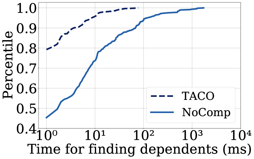
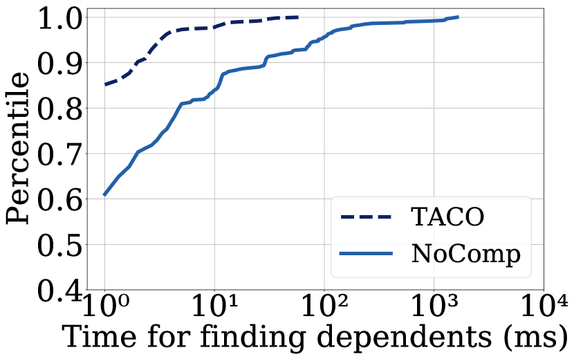
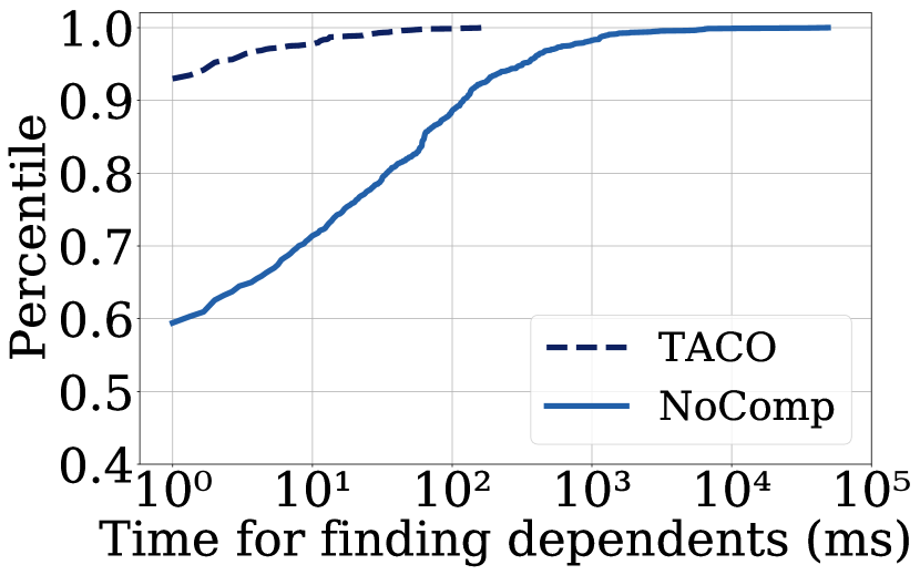
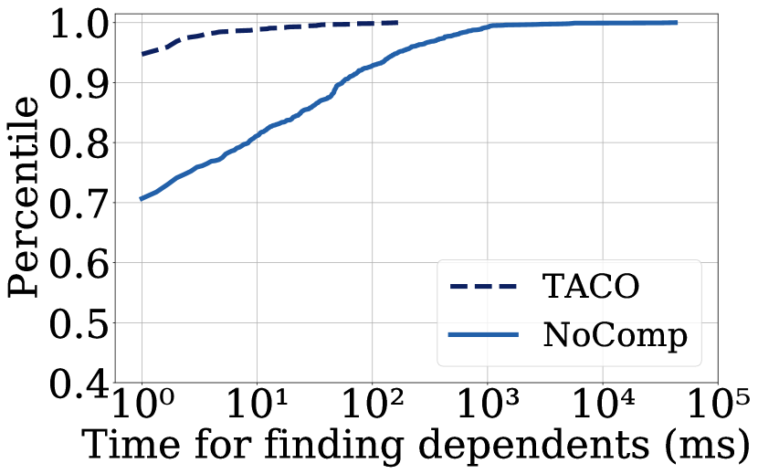
(a) Maximum Dependents (Enron) (b) Longest Path (Enron) (c) Maximum Dependents (Github) (d) Longest Path (Github)

Figure 10: CDFs for the time for finding dependents

(a) Enron (b) Github Figure 11: CDFs for the time for building formula graphs (a) Enron (b) Github Figure 12: CDFs for the time for modifying formula graphs

VI-B Compressed Formula Graph Sizes

We first test the effectiveness of TACO in reducing the graph sizes. We test two variants: TACO-InRow and TACO-Full. TACO-InRow only compresses adjacent column formulae that reference ranges in the same row, using RR to perform the compression. This approach captures the pattern of derived columns, where a subset of columns are computed using the remaining, which is common in data science and feature engineering (e.g., storing normalized versions of values in a column as a new column, or extracting substrings of an existing column and storing them as a new column). TACO-Full considers any formulae and adopts all predefined patterns.

Overall effectiveness of reducing graph sizes We first report the total number of vertices and edges of the compressed and uncompressed formula graphs across all the files in Enron and Github, respectively, in Table II. The uncompressed graphs are built using NoComp, as discussed in Sec. IV-D. Both TACO-InRow and TACO-Full significantly reduce the total number of vertices and edges compared to NoComp. For example, TACO-Full reduces the number of edges in Github from 179.8M to 3.5M. In addition, TACO-Full has much smaller graph sizes than TACO-InRow (e.g., 3.5M vs. 55.2M edges for Github), which shows that many formulae reference different rows and TACO-Full can efficiently compress these complex cases that TACO-InRow does not consider.

To further understand the effectiveness of TACO, we compute two additional metrics for each spreadsheet’s uncompressed formula graph $G^{\prime}(E^{\prime},V^{\prime})$ and compressed formula graph $G(E,V)$: the number of edges reduced by the TACO (i.e., $|E^{\prime}|-|E|$) and the fraction of the number of compressed edges compared to the uncompressed ones (i.e., $\frac{|E|}{|E^{\prime}|}$). Table III reports the max, 75th percentile, median, and mean value of the number of reduced edges across all files for both datasets. Table IV reports the min, 25th percentile, median, and mean value of the edge fraction after compression.

Table III shows that TACO-Full can reduce the number of edges by up to 700K and 3.1M in a single spreadsheet for Enron and Github, respectively. The average edge reduction by TACO-Full is 38K and 79K for the two datasets. Table IV shows that the average edge fractions after compression by TACO-Full are as low as 7.4% and 3.4% for Enron and Github, respectively. These results show that TACO can effectively reduce formula graph sizes of real spreadsheets.

Effectiveness of TACO patterns Next, we evaluate the effectiveness of each TACO pattern in reducing the number of edges. Recall that a partition of edges $E^{\prime}_{i}$ in the original uncompressed graph $G^{\prime}(E^{\prime},V^{\prime})$ corresponds to one compressed edge $e_{i}$ in $G(E,V)$ in TACO. So the number of reduced edges of a pattern $p$ in $G$ is computed as: $\sum_{e_{i}\in E}[e_{i}.meta.p=p](|E^{\prime}_{i}|-1)$, where $[e_{i}.meta.p=p]$ considers the compressed edges for the pattern $p$, $E^{\prime}_{i}$ is the set of edges that are compressed into $e_{i}$, and $|E^{\prime}_{i}|-1$ is the number of reduced edges by $e_{i}$. We compute the above metric for each pattern, and report the total and maximum number of reduced edges across the tested spreadsheets.

The results in Table V show that RR and FF compress the most edges. The number of edges reduced by RR is more than 17.4M and 141.9M for Enron and Github, respectively. FF reduces around 3.8M and 24.8M edges in total for the two respective datasets. Other patterns also reduce a significant number of edges in some spreadsheets. For example, in the Github dataset RR-Chain reduces the number of edges up to around 400K for a single spreadsheet. FR and RF, while not as common, can reduce up to around 39K and 10K edges for a single spreadsheet, respectively. These results show that TACO’s patterns are prevalent in real spreadsheets and can significantly reduce graph sizes.

Figure 13: Latency on building graphs (Antifreeze and RedisGraph) Figure 14: Latency on finding dependents (Antifreeze and RedisGraph)

Figure 15: Latency on modifying graphs (Antifreeze and RedisGraph) Figure 16: Latency on finding dependents (Excel and NoComp-Calc)

VI-C Performance Comparison with NoComp

We now compare the performance of TACO and NoComp, including the time for finding dependents, building formula graphs, and modifying formula graphs. We focus on finding dependents because finding precedents is the dual problem.

Finding dependents For each spreadsheet we test two cases: finding dependents for the cell that has the maximum number of dependents (denoted as the Maximum Dependents case) and the cell that has the longest path (denoted as the Longest Path case) in the uncompressed graph. Recall that we consider both direct and indirect dependents of a cell for finding dependents. Fig. 10 reports the CDFs for the time of finding dependents for the two cases in the two datasets. We see that TACO has much smaller execution time for finding dependents than NoComp. For Enron and Github datasets, TACO’s maximum execution time for finding dependents is 78 ms and 167 ms, respectively, while NoComp’s maximum execution time is 1,730 ms and 48,889 ms, respectively. Across all of the tested spreadsheets, the speedup of TACO over NoComp is up to 34,972$\times$.

Building and modifying formula graphs We also test the time for building and modifying formula graphs for the two datasets. To modify a formula graph of a spreadsheet, we remove the content of a column of 1K cells starting from the cell that has the most dependents.

Fig. 12 reports the CDFs for the time of building formula graphs in two datasets. We see TACO takes more time to build the formula graphs compared to NoComp due to the compression overhead. For Enron, the longest time for building a formula graph for TACO and NoComp is 16,626 ms and 7,704 ms, respectively. For Github, this number for TACO and NoComp is 82,567 ms and 40,103 ms, respectively. We believe this overhead is acceptable because building formula graphs only happens once when we load the spreadsheet, and it can be executed in the background asynchronously and will not be on the critical path of users interacting with the system. Fig. 12 reports the CDFs for the time taken to modify formula graphs. We see that for the easy cases composing the first 90% with less than 10 ms, TACO takes more time to modify formula graphs than NoComp. For the harder cases, TACO takes less time than NoComp, which is consistent with our complexity analysis. For example, for Github, the 99th percentiles for TACO and NoComp are 33 ms and 41 ms, respectively.

VI-D Performance Comparison with Antifreeze and RedisGraph

We now compare TACO with an approach that involves compressing formula graphs, Antifreeze [7], and another approach that instantiates formula graphs in a graph database, RedisGraph [30], without compression. Antifreeze builds an uncompressed formula graph for the input dependencies, pre-computes the dependents for each cell, compresses the dependents for each cell via bounding ranges, and stores each cell along with the compressed dependents in a look-up table. If formula cells are changed, it modifies the uncompressed graph and builds the look-up table from scratch. The number of bounding ranges is set to 20, as in the original paper [7]. To store formula graphs in RedisGraph, we decompose each edge that involves a range in the original formula graph into multiple edges that only involve cells, since RedisGraph and other graph databases do not support finding overlapping vertices for an input range. For example, an edge $\textsf{\small A1:A2}\rightarrow\textsf{\small B1}$ is decomposed into two edges $\textsf{\small A1}\rightarrow\textsf{\small B1}$ and $\textsf{\small A2}\rightarrow\textsf{\small B1}$. To efficiently load a formula graph in RedisGraph, we write these decomposed edges into a CSV file and adopt RedisGraph’s bulk-load tool [31] to load this file rather than inserting each edge one by one. We use Cypher [32], a declarative graph query language, to query and maintain the graph.

For this test, we choose the top 10 spreadsheets for which TACO has the longest time for building formula graphs from each dataset . We rename top 10 spreadsheets to $max_{i}$, where $i$ represents the order. If the time for building a formula graph is greater than 300 seconds, this test is regarded as did not finish (DNF). For RedisGraph, we mark the test for finding dependents as DNF if it cannot finish within 60 seconds since we observed that the memory consumption grows quickly when finding dependents in RedisGraph. This is because RedisGraph does not efficiently optimize the declarative Cypher query and needs to search one edge multiple times. In the experiment figures, we use a red X to represent DNF.

Fig. 16-16 report the time for finding dependents of the cell that has the maximum number of dependents, and the time for building and modifying a formula graph. We see that Antifreeze only finishes building the compressed formula graph for 4 out of the 20 spreadsheets and so its other numbers are not reported (marked with X). For the spreadsheets where Antifreeze can finish the tests, TACO has the same execution time for finding dependents as Antifreeze, and has much smaller execution time for building and modifying a formula graph than Antifreeze. RedisGraph cannot finish in many tests, either, mainly due to the large graphs that only include cell-to-cell edges. Among the tests where RedisGraph finishes, TACO has much smaller execution time than RedisGraph in most of these tests. Specifically, the speedup of TACO over RedisGraph on finding dependents is up to 19,555$\times$.

VI-E Performance Comparison with Excel and NoComp-Calc

We now compare TACO’s performance of finding dependents with Excel and a baseline derived from OpenOffice Calc [6], denoted NoComp-Calc. For Excel, we test the VBA API for finding the dependents of a cell [15]. For NoComp-Calc, we implemented it based on a document that describes the design of formula graphs in OpenOffice Calc [6]. Similar to NoComp, this baseline does not compress dependencies. The difference from NoComp is that NoComp-Calc does not use an R-Tree to find the vertices in formula graphs that overlap with an input range. Instead, it pre-partitions the spreadsheet space into containers, stores overlapping ranges in each container, and uses containers to find the overlapping vertices. We use top 10 spreadsheet files for which TACO spends the most time for finding dependents in each dataset from Sec. VI-C. We rename the 10 spreadsheets to $max_{i}$, where $i$ represents the order. In each spreadsheet, we test the time for finding dependents of the cell that has the maximum number of dependents. If a test cannot finish within 300 seconds, it is marked as a red X. These experiments are done on a laptop that has one Intel Core i5 CPU with 4 physical cores and 8 GB of memory, and uses Windows 10 as the OS.

The results in Fig. 16 show that TACO is much faster than Excel in all cases. The longest time for finding dependents for TACO and Excel is 442 ms and 79,761 ms, respectively. The speedup of TACO over Excel is up to 632$\times$ (i.e., max4 from Enron). It is surprising that Excel takes longer time for finding dependents than NoComp in all cases. One possible reason is that Excel compresses formula graphs to reduce memory consumption, which introduces the overhead of decompression when the formula graphs are used for finding dependents. We note that since Excel is a complex system, it may have the overhead that TACO does not. It is also possible that Excel is optimized for other scenarios by sacrificing the performance of finding dependents. For NoComp-Calc, it cannot finish in two cases. For the other cases, TACO is much faster than NoComp-Calc and the speedup of TACO over NoComp-Calc is up to 1,682$\times$.

VII Related Work

TACO is related to formula computation, graph compression, column-oriented databases, and scalable spreadsheets.

Formula computation in spreadsheets There has been some work on improving the interactivity of spreadsheets during updates. Excel [5] and other spreadsheet systems [33, 34, 6] track dependents of formula cells to quickly identify the cells impacted by an update and recalculate them. DataSpread approaches this problem using asynchronous execution  [35, 36, 37]. It uses the formula graph to identify the impacted formula cells and mark them dirty, return control to users immediately, and calculate the dirty cells asynchronously [7]. Unlike TACO, none of these approaches leverage tabular locality to compress formula graphs. In addition, TACO is orthogonal to the execution models and can be integrated into an existing spreadsheet system to improve interactivity.

Graph compression Graph compression has been studied in many scenarios, such as in the Web [38] and social networks [39]. A recent survey [18] shows that different compression methods are designed for different goals, including understanding the structure of a graph [40], reducing graph sizes with bounded errors [41], or accelerating queries on graphs [42]. None of these papers leverage tabular locality and consider the spatial nature of formula graphs. In addition, most of them do not support directly querying the compressed graph. Fan et al. [19] support directly executing reachability and pattern matching queries on a compressed graph, but do not leverage tabular locality and support finding dependents/precedents. While a recent paper proposes a compressed graph for spreadsheets [7], we showed that building such a compressed graph is time-consuming.

Column-oriented databases Column-oriented databases [21, 20] employ lightweight compression for data in each column and execute queries directly on the compressed data without decompression [43]. TACO is instead designed to compress dependencies (i.e., edges) while column-oriented compression methods are used to compress columnar data. In addition, column-oriented databases do not consider decomposing complex patterns in a column of formulae into predefined patterns as TACO proposes.

Spreadsheets at scale Many prior papers focus on supporting large-scale data analysis on spreadsheets  [44, 45, 46, 26, 27, 47, 48, 49]. DataSpread [26, 27] adopts databases as a scalable back-end. ABC [45] provides a spreadsheet interface and uses approximate query processing techniques, such as online aggregation [50], to quickly return results. Mondrian [49] maps spreadsheets to visual images to detect different regions in spreadsheets and extract layout templates, but does not consider formula dependency compression. TACO is different from these papers because it approaches the scalability problem using compression techniques.

VIII Conclusion

We presented TACO—a framework that efficiently compresses formula graphs in spreadsheets to improve interactivity. TACO exploits tabular locality, wherein cells close to each other have formulae with similar structures, and represents tabular locality via four basic and one extended patterns. As part of TACO, we introduce algorithms for building the compressed formula graph based on predefined patterns, querying this graph without decompression, and incremental maintenance. Our experiments show that TACO can quickly find the dependents of spreadsheet cells to significantly reduce the time of returning control to users while achieving fast graph maintenance at the same time.

References

- [1] Microsoft UK Enterprise Team, “How finance leaders can drive performance,” https://enterprise.microsoft.com/en-gb/articles/roles/finance-leader/how-finance-leaders-can-drive-performance/, 2015.
- [2] “Excel vs. Google Sheets usage — nature and numbers,” https://medium.com/grid-spreadsheets-run-the-world/excel-vs-google-sheets-usage-nature-and-numbers-9dfa5d1cadbd, 2018.
- [3] B. A. Nardi and J. R. Miller, The spreadsheet interface: A basis for end user programming. Hewlett-Packard Laboratories, 1990.
- [4] A. Gupta, I. S. Mumick, and V. S. Subrahmanian, “Maintaining views incrementally,” in Proceedings of the 1993 ACM SIGMOD International Conference on Management of Data, Washington, DC, USA, May 26-28, 1993, 1993, pp. 157–166. [Online]. Available: http://doi.acm.org/10.1145/170035.170066
- [5] C. Williams et al., “Excel performance: Improving calculation performance,” https://docs.microsoft.com/en-us/office/vba/excel/concepts/excel-performance/excel-improving-calcuation-performance, 2017.
- [6] “Calc formula dependence,” https://wiki.openoffice.org/wiki/Calc/Implementation/Formula_cell_and_cells_dependence.
- [7] M. Bendre, T. Wattanawaroon, K. Mack, K. Chang, and A. G. Parameswaran, “Anti-freeze for large and complex spreadsheets: Asynchronous formula computation,” in Proceedings of the 2019 International Conference on Management of Data, SIGMOD Conference 2019, Amsterdam, The Netherlands, June 30 - July 5, 2019, P. A. Boncz, S. Manegold, A. Ailamaki, A. Deshpande, and T. Kraska, Eds. ACM, 2019, pp. 1277–1294. [Online]. Available: https://doi.org/10.1145/3299869.3319876
- [8] “Display the relationships between formulas and cells,” https://support.microsoft.com/en-us/office/display-the-relationships-between-formulas-and-cells-a59bef2b-3701-46bf-8ff1-d3518771d507.
- [9] “Trace Dependents,” https://help.libreoffice.org/latest/lo/text/scalc/01/06030300.html.
- [10] “EuSpRIG Horror Stories,” http://www.eusprig.org/horror-stories.htm.
- [11] R. R. Panko, “What we don’t know about spreadsheet errors today: The facts, why we don’t believe them, and what we need to do,” CoRR, vol. abs/1602.02601, 2016. [Online]. Available: http://arxiv.org/abs/1602.02601
- [12] “Excel Formula Precedents and Dependents Navigator,” https://www.breezetree.com/excel-utilities/formula-dependency-audit.
- [13] B. Klimt and Y. Yang, “Introducing the enron corpus.” in CEAS, 2004.
- [14] Z. Liu and J. Heer, “The effects of interactive latency on exploratory visual analysis,” IEEE Trans. Vis. Comput. Graph., vol. 20, no. 12, pp. 2122–2131, 2014.
- [15] “Range.Dependents,” https://docs.microsoft.com/en-us/office/vba/api/excel.range.dependents.
- [16] “Apache POI,” https://poi.apache.org/.
- [17] M. R. Garey and D. S. Johnson, Computers and Intractability: A Guide to the Theory of NP-Completeness. W. H. Freeman, 1979.
- [18] Y. Liu et al., “Graph summarization methods and applications: A survey,” ACM Computing Surveys (CSUR), vol. 51, no. 3, p. 62, 2018.
- [19] W. Fan, J. Li, X. Wang, and Y. Wu, “Query preserving graph compression,” in Proceedings of the ACM SIGMOD International Conference on Management of Data, SIGMOD 2012, Scottsdale, AZ, USA, May 20-24, 2012, K. S. Candan, Y. Chen, R. T. Snodgrass, L. Gravano, and A. Fuxman, Eds. ACM, 2012, pp. 157–168. [Online]. Available: https://doi.org/10.1145/2213836.2213855
- [20] P. A. Boncz, M. Zukowski, and N. Nes, “Monetdb/x100: Hyper-pipelining query execution,” in Second Biennial Conference on Innovative Data Systems Research, CIDR 2005, Asilomar, CA, USA, January 4-7, 2005, Online Proceedings. www.cidrdb.org, 2005, pp. 225–237. [Online]. Available: http://cidrdb.org/cidr2005/papers/P19.pdf
- [21] M. Stonebraker, D. J. Abadi, A. Batkin, X. Chen, M. Cherniack, M. Ferreira, E. Lau, A. Lin, S. Madden, E. J. O’Neil, P. E. O’Neil, A. Rasin, N. Tran, and S. B. Zdonik, “C-store: A column-oriented DBMS,” in Proceedings of the 31st International Conference on Very Large Data Bases, Trondheim, Norway, August 30 - September 2, 2005, K. Böhm, C. S. Jensen, L. M. Haas, M. L. Kersten, P. Larson, and B. C. Ooi, Eds. ACM, 2005, pp. 553–564. [Online]. Available: http://www.vldb.org/archives/website/2005/program/paper/thu/p553-stonebraker.pdf
- [22] “CellFormula,” https://docs.microsoft.com/en-us/dotnet/api/documentformat.openxml.spreadsheet.cellformula?view=openxml-2.8.1.
- [23] A. Guttman, “R-trees: A dynamic index structure for spatial searching,” in SIGMOD, 1984.
- [24] “Absolute and Relative References,” https://support.microsoft.com/en-us/office/switch-between-relative-absolute-and-mixed-references-dfec08cd-ae65-4f56-839e-5f0d8d0baca9.
- [25] “Bell Number,” https://en.wikipedia.org/wiki/Bell_number.
- [26] M. Bendre et al., “Dataspread: Unifying databases and spreadsheets,” in VLDB, 2015.
- [27] M. Bendre, V. Venkataraman, X. Zhou, K. C. Chang, and A. G. Parameswaran, “Towards a holistic integration of spreadsheets with databases: A scalable storage engine for presentational data management,” in 34th IEEE International Conference on Data Engineering, ICDE 2018, Paris, France, April 16-19, 2018. IEEE Computer Society, 2018, pp. 113–124. [Online]. Available: https://doi.org/10.1109/ICDE.2018.00020
- [28] M. Bendre et al., “Faster, higher, stronger: Redesigning spreadsheets for scale,” in ICDE, 2019.
- [29] “TACO Lens,” https://github.com/taco-org/tacolens.
- [30] “Redisgraph,” https://redis.io/docs/stack/graph/.
- [31] “Redisgraph-bulk-loader,” https://github.com/RedisGraph/redisgraph-bulk-loader.
- [32] “Cyhper (query language),” https://en.wikipedia.org/wiki/Cypher_(query_language).
- [33] P. Sestoft, Spreadsheet Implementation Technology: Basics and Extensions. The MIT Press, 2014.
- [34] “ZK Spreadsheet,” https://www.zkoss.org/product/sheet.
- [35] A. Marcus et al., “Crowdsourced databases: Query processing with people,” in CIDR, 2011.
- [36] A. G. Parameswaran et al., “Deco: declarative crowdsourcing,” in CIKM, 2012.
- [37] S. Brin and L. Page, “The anatomy of a large-scale hypertextual web search engine,” Computer networks, vol. 30, no. 1-7, pp. 107–117, 1998.
- [38] P. Boldi and S. Vigna, “The webgraph framework I: compression techniques,” in Proceedings of the 13th international conference on World Wide Web, WWW 2004, New York, NY, USA, May 17-20, 2004, S. I. Feldman, M. Uretsky, M. Najork, and C. E. Wills, Eds. ACM, 2004, pp. 595–602. [Online]. Available: https://doi.org/10.1145/988672.988752
- [39] F. Chierichetti, R. Kumar, S. Lattanzi, M. Mitzenmacher, A. Panconesi, and P. Raghavan, “On compressing social networks,” in Proceedings of the 15th ACM SIGKDD International Conference on Knowledge Discovery and Data Mining, Paris, France, June 28 - July 1, 2009, J. F. E. IV, F. Fogelman-Soulié, P. A. Flach, and M. J. Zaki, Eds. ACM, 2009, pp. 219–228. [Online]. Available: https://doi.org/10.1145/1557019.1557049
- [40] R. Cilibrasi and P. Vitanyi, “Clustering by compression,” IEEE Transactions on Information Theory, vol. 51, no. 4, pp. 1523–1545, 2005.
- [41] S. Navlakha et al., “Graph summarization with bounded error,” in SIGMOD, 2008.
- [42] A. Maccioni and D. J. Abadi, “Scalable pattern matching over compressed graphs via dedensification,” in KDD, 2016.
- [43] D. J. Abadi, S. Madden, and M. Ferreira, “Integrating compression and execution in column-oriented database systems,” in Proceedings of the ACM SIGMOD International Conference on Management of Data, Chicago, Illinois, USA, June 27-29, 2006, S. Chaudhuri, V. Hristidis, and N. Polyzotis, Eds. ACM, 2006, pp. 671–682. [Online]. Available: https://doi.org/10.1145/1142473.1142548
- [44] “1010 Data,” https://www.1010data.com/.
- [45] V. Raman et al., “Scalable spreadsheets for interactive data analysis.” in DMKD, 1999.
- [46] “Airtable,” https://www.airtable.com/.
- [47] A. Witkowski et al., “Advanced SQL modeling in RDBMS,” TODS, vol. 30, no. 1, pp. 83–121, 2005.
- [48] A. Witkowsk et al., “Query by excel,” in VLDB, 2005.
- [49] G. Vitagliano, L. Jiang, and F. Naumann, “Detecting layout templates in complex multiregion files,” Proc. VLDB Endow., vol. 15, no. 3, pp. 646–658, 2021. [Online]. Available: http://www.vldb.org/pvldb/vol15/p646-vitagliano.pdf
- [50] V. Raman, B. Raman, and J. M. Hellerstein, “Online dynamic reordering for interactive data processing,” in VLDB, vol. 99, 1999, pp. 709–720.