Transactional Panorama: A Conceptual Framework for
User Perception in Analytical Visual Interfaces

Abstract.

Many tools empower analysts and data scientists to consume analysis results in a visual interface. When the underlying data changes, these results need to be updated, but this update can take a long time—all while the user continues to explore the results. Tools can either (i) hide away results that haven’t been updated, hindering exploration; (ii) make the updated results immediately available to the user (on the same screen as old results), leading to confusion and incorrect insights; or (iii) present old—and therefore stale—results to the user during the update. To help users reason about these options and others, and make appropriate trade-offs, we introduce Transactional Panorama, a formal framework that adopts transactions to jointly model the system refreshing the analysis results and the user interacting with them. We introduce three key properties that are important for user perception in this context: visibility (allowing users to continuously explore results), consistency (ensuring that results presented are from the same version of the data), and monotonicity (making sure that results don’t “go back in time”). Within transactional panorama, we characterize all feasible property combinations, design new mechanisms (that we call lenses) for presenting analysis results to the user while preserving a given property combination, formally prove their relative orderings for various performance criteria, and discuss their use cases. We propose novel algorithms to preserve each property combination and efficiently present fresh analysis results. We implement our framework into a popular, open-source BI tool, illustrate the relative performance implications of different lenses, and demonstrate the benefits of the novel lenses and our optimizations.

1. Introduction

Many data-centric tools empower a user to visually organize, present, and consume multiple data analysis results within a single interface, such as a dashboard. Each such analysis result is represented on this interface as a scalar value, table, or visualization, and is computed using the source data or other analysis results, in turn, as views. This pattern appears in a variety of contexts:

Visual analytics or Business Intelligence (BI) tools, like Tableau (tableau, ) or PowerBI (powerBI, ), empower a user to embed visualizations on a dashboard, each via a SQL query on an underlying database;

Spreadsheet tools, such as Microsoft Excel (msexcel, ) and Google Sheets (sheets, ), allow a user to add derived computation in the form of spreadsheet formulae, visualizations, and pivot tables;

Data application builder tools, such as Streamlit (streamlit, ), Plotly (plotly, ), and Redash (redash, ), enable a user to efficiently develop interactive dashboards, employing computation done in Python UDFs and pandas dataframe functions, and SQL; and

Monitoring and observability tools, such as Datadog (datadog, ), Kibana (kibana, ), and Grafana (grafana, ), empower a user to make sense of their telemetry data and logs via a combination of automatically defined and customizable dashboard widgets.

In all of these contexts, there is a network of views defined on underlying data, each of which is then visualized on an interface. These views and the corresponding visualizations often need to be refreshed when the source data is modified. For example, a dashboard in a BI tool is refreshed with respect to regular changes to the underlying database tables (e.g., new batches of data). However, this refresh is rarely instantaneous, especially on large datasets. This represents a challenge, since the user is continuously exploring the visualizations during the refresh. On the one hand, refreshing visualizations arbitrarily can be jarring to the user, since different visualizations on the screen may be in different stages of being refreshed. On the other hand, not refreshing them in a timely manner can lead to stale results. The question we explore is: How do we allow users to continuously explore results in a visual interface, while ensuring that the results are not confusing or stale?

Lens name	Example Tools	Monotonicity	Visibility	Consistency
Globally-Consistent Fully-Blocking (GCFB)	MS Excel (msexcel, ) Libre Calc (libreCalc, ) Tableau (tableau, )	Yes	No	Yes
Globally-Consistent Partially-Blocking (GCPB)	Power BI (powerBI, ) Superset (superset, ) Dataspread (Antifreeze, )	Yes	No	Yes
Inconsistently Non-Blocking (ICNB)	Google Sheets (sheets, )	Yes	Yes	No

Table 1. Properties maintained by existing tools

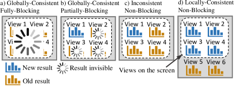
Figure 1. Visual examples of different lenses for refreshing views in a dashboard

Unfortunately, existing tools make fixed, and somewhat arbitrary decisions on how to address this question. For example, Excel (msexcel, ), Calc (libreCalc, ), and Tableau (tableau, ) block the user from exploring the interface until all of the views are refreshed (Figure 1a). Other tools, like PowerBI (powerBI, ), Superset (superset, ), and Dataspread (Antifreeze, ), improve on this approach by hiding (or greying) away any views that have not yet been refreshed, while still letting the user explore the other up-to-date views (Figure 1b). Yet other tools, like Google Sheets (sheets, ), opt for not hiding any views, and instead just progressively make them available as they are refreshed—this approach has the downside of different results on the screen being in different stages of being refreshed, leading to incorrect insights (Figure 1c).

Transactional Panorama and Underlying Properties. In this paper, we introduce a formal framework, named transactional panorama, to enable users and system designers to reason about the aforementioned question in a more principled manner. We adopt transactions to jointly model the system concurrently updating visualizations, with the user consuming these visualizations, over time and space (i.e., across screens). To the best of our knowledge, transactional panorama is the first framework that leverages transactions to reason about correct user perception in visual interfaces. In this setting, we define three key desirable properties monotonicity, visibility, and consistency, which we call the MVC properties. Monotonicity guarantees that if a user reads the result for a view, any subsequent read will always return the same or more recent result (i.e., monotonic read (DSBook, )) so that results never go “back in time”. Visibility guarantees that the user can always explore the result of any visualization on the screen—instead of them being greyed out. Consistency guarantees that the results displayed on the screen should be consistent with the same snapshot of source data (GolabJ11Consistency, ; ZhugeGW97Multiview, )—enabling correct derivation of relationships between results on the same screen.

Concrete Property Combinations via Lenses. There are various mechanisms we can use to present results to the user in a visual interface, resulting in concrete selections for the aforementioned properties, that we call lenses. Consider our examples of existing systems (Figure 1a–c); we list the corresponding three lenses in Table 1—GCFB, GCPB, and ICNB (the acronyms will be explained later). While GCFB and GCPB opt for monotonicity and consistency, instead of visibility, ICNB opts for monotonicity and visibility, but not consistency. In this work, we study the feasibility of different property combinations and lenses, and characterize their performance trade-offs. In particular, we explore the trade-off between invisibility, i.e., the duration when the user is unable to interact with visualizations, and staleness, i.e., the duration when visualizations displayed to the user have not been refreshed, as shown in Figure 2. For example, GCFB blocks the user from exploring the interface until all of the new results are computed, so it has high invisibility. But GCFB also has zero staleness since it does not present stale results. On the other hand GCPB reduces invisibility (vs. GCFB) by presenting the newly computed results to the user whenever available while also not showing stale results. ICNB, which sacrifices consistency, has higher staleness because the user can read stale results, but none of the views shown are invisible, i.e., visualizations that are greyed out.

Novel Property Combinations: Exploring the Trade-off. As we also show in Figure 2 (in green), we discover a number of novel lenses, resulting in new property combinations and associated performance implications. We introduce three new lenses: Globally-Consistent Non-Blocking (GCNB), Locally-Consistent Non-Blocking (LCNB), and Locally-Consistent Minimum-Blocking (LCMB), none of which are dominated by the three existing lenses. For example, LCNB always allows the user to inspect the results of any visualizations (i.e., preserving visibility), and refreshes the visualizations on the screen when all of their new results are computed (i.e., preserving consistency). Figure 1d shows an example of LCNB, where the user can quickly read the new results on the screen (i.e., $View_{1-4}$) without waiting for computing the new results that are not on the current screen (i.e., $View_{5-6}$). LCNB can be used when a user wants to always see and interact with consistent results on the screen. However, as we prove later, LCNB needs to sacrifice monotonicity when the user explores different visualizations (e.g., by scrolling). In fact, we demonstrate one can achieve both consistency and visibility simultaneously only by either sacrificing monotonicity or suffering from high staleness. For the aforementioned new lenses, we further introduce $k$-relaxed variants (i.e., $k$-GCNB, $k$-LCNB, and $k$-LCMB), where $k$ represents the number of additional invisible views allowed for each lens.

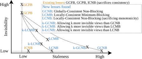
Figure 2. Trade-off between invisibility and staleness across different lenses

Usage Scenarios. This suite of lenses allow a user or a system designer to determine their desired properties and gracefully explore the trade-off between staleness and invisibility. Current tools, while enabling users to customize their dashboards extensively (in terms of the placement of visualizations and selection of visualization queries and encodings), make fixed choices in this regard. A user has no say in how results are refreshed and presented, and a system designer opts for whatever is easiest. The transactional panorama framework is intended to address this gap. From an end-user standpoint, they may be able to make appropriate performance trade-offs via various customization knobs. A system designer may similarly be able to make appropriate selections during tool design, with end-users and use-cases in mind.

Translating to Practice: Challenges. Translating our transactional panorama framework to practice in real data analysis and BI systems requires addressing several challenges:

(1) In a visual interface, the user does not explicitly submit transactions as in traditional systems, but reads the views by looking at the screen. In addition, the user can read different subsets of views by scrolling to different screens. Therefore, a challenge is to adapt transactions to model user behavior, an aspect not considered in classical transaction processing literature.

(2) In a visual interface, the user may want to quickly read new results for some views before the system computes all of the new results. If we model an update along with refreshing the related views as a transaction (to preserve consistency), the user essentially wants to read the results of an uncommitted transaction. The MVC properties for reading uncommitted results are not considered by traditional systems and needs to be defined in our model.

(3) Finally, instantiating transactional panorama requires designing new algorithms for efficiently maintaining different property combinations for different lenses while reducing invisibility and staleness. Traditional concurrency control protocols, such as 2PL or OCC (BernsteinHG87CCBook, ), do not apply here because they do not consider maintaining consistency on uncommitted results and the other user-facing properties, monotonicity and visibility.

Summary of Contributions. We address these challenges as part of transactional panorama and make the following contributions:

• We present the transactional panorama model in Section 2. We model reads and writes on the views as operations within transactions and introduce a special read-only transaction to model a user’s behavior of reading the views on the screen. We define the MVC properties and use a series of theorems to exhaustingly explore the possible property combinations. We formally order different lenses based on invisibility and staleness, and provide guidance for selecting the right lens for specific use cases.

• We design efficient algorithms for maintaining properties for lenses in Section 3, and propose optimizations to reduce invisibility and staleness while refreshing analysis results in Section 4.

• We implement transactional panorama within Apache Superset, a popular open-source BI tool (superset, ), in Section 5. We perform extensive experiments to characterize the relative benefits of different lenses on various workloads, demonstrate the benefits of the new lenses, and show the performance benefit of our optimizations on reducing invisibility and staleness compared to the baselines—by up to 70% and 75%, respectively—in Section 6.

2. Transactional Panorama model

We present our transactional panorama model in this section. We introduce various key concepts in Section 2.1. Then, we discuss modeling reading/writing views using transactions in Section 2.2. Next, we formalize our model in Section 2.3, define the MVC properties in Section 2.4, and evaluate the feasibility of various property combinations in Section 2.5. We introduce new property combinations and the corresponding lenses in Section 2.6. Afterwards, we define performance metrics in Section 2.7 and order the lenses by the performance metrics in Section 2.8. Finally, we discuss selecting appropriate lenses for specific use cases in Section 2.9 and extensions of the model in Section 2.10.

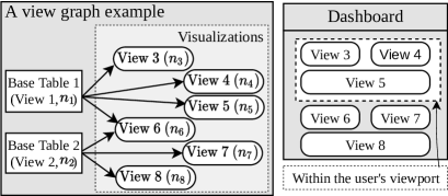
Figure 3. An example of a dashboard and its view graph

2.1. Preliminaries

View and view graph. In our context, we define a view to represent arbitrary computation, expressed in any manner, including SQL, pandas dataframe expressions, spreadsheet formulae, or UDFs, taking other views and/or source data as input. A view graph is a directed acyclic graph (DAG) that captures the dependencies across views and source data, both represented as nodes in the DAG. Specifically, if a view $n_{i}$ takes another view or source data $n_{j}$ as input, we add an edge: $n_{j}$ $\rightarrow$ $n_{i}$. The dependents of $n_{j}$ are defined as the views that are reachable from $n_{j}$ in the view graph. For simplicity, we regard the source data as a special type of view that performs an identity function over the source data. Figure 3 shows an example of a view graph for visualizations in a dashboard, where the source data are database tables and each view is defined by a SQL statement. There are two base tables: Base Table 1 and 2, also regarded as View 1 and 2, respectively. We use $n_{k}$ to represent View k. View 3-6 (denoted $n_{3-6}$) and View 6-8 (denoted $n_{6-8}$) are the dependents of $n_{1}$ and $n_{2}$, respectively. They define the content for the visualizations in this dashboard.

Notations	Meanings
$w^{t_{i}}$	A write transaction that is created at timestamp $t_{i}$
$r^{s_{i}}$	A read transaction that is created at timestamp $s_{i}$
$G^{t_{i}}$	A version of the view graph created by $w^{t_{i}}$
$n_{k}$	A view in the view graph
$n_{k}^{t_{i}}$	A view result for $n_{k}$ in $G^{t_{i}}$
$UC^{t_{i}}_{k}$	A state representing the view result $n_{k}^{t_{i}}$ is under computation
$V^{t_{i}}$	A set that stores the view results and UCs for the views in $G^{t_{i}}$
$C_{f}$	Consistency-fresh
$C_{m}$	Consistency-minimal
$C_{c}$	Consistency-committed

Table 2. Notation frequently used in this paper

View result and viewport. A view result represents the output of a view given a version of the source data and the definition of the view graph. This view result is rendered on the dashboard as a visualization (this includes visualizations of tables or even single values). In certain settings, a view definition may itself be editable and rendered as part of the dashboard (e.g., as a filter). For the following discussion, we assume view definitions are not editable or rendered. We discuss reading and modifying a view definition in Section 2.10. A dashboard may include many visualizations that cannot fit into a single screen. The rectangular area on the screen a user is currently looking at is the viewport. In Figure 3, the viewport includes visualizations for views $n_{3-5}$. A user can change the viewport to explore different parts of a view graph.

Reading and writing a view, and view state. We model the user inspecting a visualization in the viewport as reading the corresponding view, which returns a view state. A view state is either a view result or a state that indicates the view result has not been computed yet (denoted as under-computation) and is usually materialized such that future reads coming from the user can reuse the materialized state. In Figure 3, we need to materialize the view states for $n_{3-8}$ to support future reads by the user.

There are two types of writes in transactional panorama: input writes and triggered writes. An input write is from a user or an external system, and modifies the source data (e.g., new data inserted to a base table) or view graph definitions. In the following, we focus on input writes to the source data as it is the most common case of refreshing a dashboard. We discuss processing modifications to the view graph definitions in Section 2.10. The input write will trigger additional writes, called triggered writes, which compute new results for the views that depend on the base views which were modified in the input write. For example, modifying the base table $n_{1}$ in Figure 3 triggers computing new results for $n_{3-6}$.

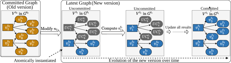
Figure 4. An example of creating a new version of view graph and computing the view result for each node

2.2. Modeling the Interaction with a View Graph

We model a user’s or an external system’s interaction with a view graph as transactions, and logically associate each transaction with a unique timestamp that represents its submission time, with transactions being ordered by these timestamps. We focus on a single user setting as in most user-facing data analysis tools, such as Excel (msexcel, ), Tableau (tableau, ), and PowerBI (powerBI, ), and discuss the multiple user setting in Section 2.10. Our model has two types of transactions:

Write transaction. A write transaction is issued when a set of input writes on the view graph (e.g., modifications to a set of base tables) are submitted together to the system. A write transaction involves processing the input writes and recomputing the views that depend on the input writes. For example, in Figure 3 if $n_{1}$ is modified the write transaction will recompute $n_{3-6}$. The specific algorithm for maintaining the view graph and recomputing view results is orthogonal to our model, and, for example, can employ incremental view maintenance (Gupta93IVM, ; DBT, ; TangSEKF20InQP, ). We focus on processing one write transaction at a time, which is typical in existing tools  (msexcel, ; tableau, ; powerBI, ; superset, ), and discuss the case of multiple, simultaneous write transactions in Section 2.10.

Read transaction. Transactional panorama models a user inspecting visualizations in the viewport as a read transaction. For example, in Figure 3, the read transaction involves reading views $n_{3-5}$. A unique property of this read transaction is that it does not delay to wait for the requested view results to be computed. So the read transaction may return an under-computation state for a visualization if the view result has not been computed yet. If an under-computation state is returned, the user cannot inspect and interact with the visualization in the visual interface. To simulate the effect of the user “looking at” the viewport, our model assumes the system periodically issues new read transactions to pull view states. The user may read different parts of the view graph by changing the viewport while the system continues to process writes. The location of the user’s viewport is known to the system throughout.

2.3. Formalization

We now introduce the aforementioned concepts in more detail and more formally. Table 2 summarizes the notation frequently used in this paper. The view graph is logically multi-versioned, where a new version of view graph $G^{t_{i}}=(E,N,V^{t_{i}})$ is instantiated by a write transaction with timestamp $t_{i}$ (denoted as $w^{t_{i}}$). $N$ represents the set of nodes (i.e., source data and views) in the graph and each edge $e={(n_{prec},n_{dep})}\in E$ indicates that node $n_{dep}$ has another node $n_{prec}$ as input. $V^{t_{i}}$ captures the view results and the under-computation states for the views in $G^{t_{i}}$ and evolves as we process the write transaction $w^{t_{i}}$. At a given time, $V^{t_{i}}$ may include: i) the view result for $n_{k}$ that $w^{t_{i}}$ has already finished computing — this view result is represented as $v^{t_{i}}_{k}$; ii) $\textsf{\small UC}^{t_{i}}_{k}$, which represents the state that $w^{t_{i}}$ intends to compute the view result for $n_{k}$, but has not done it yet; and iii) the view result for $n_{k}$ from the last version of view graph given that $n_{k}$ will not be updated by $w^{t_{i}}$. Figure 4 shows an example of computing a new version of view graph for a write transaction $w^{t_{1}}$ that modifies $n_{1}$ in Figure 3. We see that creating a new version of view graph logically replicates the view results of the last version of the view graph, and marks all of the view results to be computed as UCs (in gray). Each UC is replaced after the corresponding view result is computed (in blue). We guarantee that a new version of view graph is atomically seen by read transactions via our concurrency control protocol (to be discussed in Section 3). We call a version of view graph committed if its write transaction is committed; otherwise, this version is uncommitted. A write transaction is defined to be committed if the system has a) computed all of the new view results for the version of view graph created by this write transaction and b) updated a global variable that stores the timestamp of the recently committed graph. More details about the procedure for processing a write transaction and the management of the global variable are in Section 3.2. The initial version of the view graph is $G^{t_{0}}$, which is modified by a sequence of write transactions $W=\{w^{t_{1}},\cdots,w^{t_{n}}\}$, where $w^{t_{i}}$ is submitted before $w^{t_{j}}$ if $t_{i}<t_{j}$.

We also have a sequence of read transactions $R=\{r^{s_{1}},\cdots,r^{s_{m}}\}$, where $r^{s_{i}}$ is submitted before $r^{s_{j}}$ if $s_{i}<s_{j}$. Recall that each read transaction corresponds to a single viewport and all of the views in it. We refer to the view states returned by a read transaction $r^{s_{i}}$ as $H^{s_{i}}$, which includes view results and/or UCs for the views in the viewport. If a read transaction returns a UC for a view, its corresponding visualization is marked as invisible in the dashboard. On the front end, this can be displayed in various ways: grayed out, a progress bar, a loading sign, etc. We use UC for $\textsf{\small UC}^{t_{i}}_{k}$ when $k$ and $t_{i}$ are clear from the context.

2.4. MVC Properties

We now formally define the so-called MVC properties for read transactions, motivated by user needs in analytical visual interfaces. First, the user consumes the view states returned by read transactions in order: i.e., they consume the view states of one read transaction before the next. Therefore, they expect to see monotonically newer states for each view, avoiding the confusion that the states seen “travel back in time”. Second, in a user-facing dashboard, the notion of visibility helps ensure interactivity, as it means the user can continuously explore the view results of different visualizations without interruption, while the system processes write transactions. Finally, consistency helps ensure that insights derived from multiple visualizations on a viewport are computed from the same snapshot of source data (ZhugeGW97Multiview, ; GolabJ11Consistency, ; WuCH020InteractionSnapshots, ). We now describe each property in detail.

Monotonicity. Monotonicity means if a user reads a given version of a view result or UC for a view, any successive reads on the same view will return the same or more recent version of the view result or UC. Formally, monotonicity is defined as:

Definition 0 (Monotonicity).

A sequence of read transactions $R=\{r^{s_{1}},\cdots,r^{s_{m}}\}$ maintains monotonicity if the following holds: for any view $n_{k}$ read by any two transactions $r^{s_{i}}$ and $r^{s_{j}}$, the timestamps of the returned states are $t_{p}$ and $t_{q}$, respectively: $t_{p}\leq t_{q}$ if $s_{i}<s_{j}$.

To maintain monotonicity, the system needs to track the timestamps of the results for each view returned by the recent read operations, as will be discussed in Section 3.

Visibility. This property says that for any view that is read by any read transaction, the system should not return an under-computation state, UC. Formally, visibility is defined as:

Definition 0 (Visibility).

A sequence of read transactions $R=\{r^{s_{1}},\cdots,r^{s_{m}}\}$ maintains visibility if for the states $H^{s_{i}}$ that are returned by any transaction $r^{s_{i}}$, we have $\textsf{\small UC}\not\in H^{s_{i}}$.

The user may also sacrifice visibility by opting for partial visibility, where they accept a controlled number of UCs as a trade-off for reading fresher view results, discussed next.

Consistency. In our setting, consistency means that the view states returned by each read transaction belongs to a single version of the view graph. Consistency is formally defined as:

Definition 0 (Consistency).

Let $H^{s_{i}}$ be the view states returned by $r^{s_{i}}$. We say $r^{s_{i}}$ maintains consistency if there exists a version of view graph $G^{t_{j}}=(E,N,V^{t_{j}})$ such that $t_{j}\leq s_{i}$ and $H^{s_{i}}\subseteq V^{t_{j}}$.

Intuitively, $t_{j}\leq s_{i}$ requires that a user read a version created by the write transactions that happen before $r^{s_{i}}$. The condition $H^{s_{i}}\subseteq V^{t_{j}}$ guarantees that the view states returned belong to a single version of view graph. Consider a read transaction $r^{s_{1}}$ that reads $n_{3-5}$. Say for $G^{t_{1}}$ in Figure 3, we have computed $v_{3}^{t_{1}}$ but not $v_{4-5}^{t_{1}}$. If the returned states for $r^{s_{1}}$ is $H^{s_{1}}=\{v_{3}^{t_{1}},\textsf{\small UC}_{4-5}^{t_{1}}\}$, then $r^{s_{1}}$ maintains consistency because $H^{s_{1}}$ belongs to $V^{t_{1}}$.

Note that consistency in transactional panorama is different from traditional Consistency (C) in ACID for database transactions. C in ACID refers to the property that each transaction correctly brings the database from one valid state to another. In our context, consistency is more closely related to Isolation (I) in ACID, which defines when view results created by one transaction can be read by others. Our notion of consistency allows a read transaction to read uncommitted results from a concurrently running write transaction (e.g., reading the uncommitted $G^{t_{1}}$), but additionally maintains the semantics that the returned states correspond to a single version.

A follow-up question about preserving consistency is which version of view graph a read transaction should read. Specifically, since we process one write transaction at a time, a read transaction can choose between reading the last committed version of view graph, which we call the committed graph, and the version that the latest write transaction is computing, which we call the latest graph. Depending on the version that is read, we define three types of consistency, which opt for different trade-offs between invisibility and staleness. (Recall that invisibility refers to the time during which the views in the viewport are invisible, while staleness refers to the time during which the returned view results are not consistent with the latest graph; both will be defined in Section 2.7.)

The first type of consistency is Consistency-fresh or $C_{f}$, which always reads the latest graph. $C_{f}$ returns fresh results but suffers high invisibility. For the example in Figure 4, with $C_{f}$, read transactions always read $G^{t_{1}}$ while we are processing the write transaction.

Another type of consistency, called Consistency-committed or $C_{c}$, always reads the most recently committed graph. $C_{c}$ does not have invisible views, but the staleness of the returned view results could be high. In Figure 4, if $C_{c}$ is used, read transactions cannot read $G^{t_{1}}$ until we have computed all of the view results for $G^{t_{1}}$ (i.e., $v_{1}^{t_{1}}$ and $v_{3-6}^{t_{1}}$).

We additionally introduce a type of consistency that lies between $C_{f}$ and $C_{c}$. This type of consistency requires that a read transaction read the most recent version of the view graph that returns the minimum number of UCs for this transaction, which we call Consistency-minimal or $C_{m}$ for short. With $C_{m}$, we would typically read the committed graph to avoid returning UCs when the new view results in the viewport are not yet computed. Once they are computed, we can read the latest graph to return fresh view results. Consider reading $n_{3-5}$ in Figure 4. Initially, the read transactions will read $G^{t_{0}}$ because $G^{t_{0}}$ does not include UCs. After the new results for $n_{3-5}$ are computed, we will read $G^{t_{1}}$ because reading $G^{t_{1}}$ for $n_{3-5}$ does not return $\textsf{\small UC}{s}$, and $G^{t_{1}}$ is more recent than $G^{t_{0}}$. Note that $C_{m}$ is different from $C_{c}$ because for $C_{c}$, read transactions will read the latest graph $G^{t_{1}}$ after the write transaction is committed, while for $C_{m}$, read transactions will read $G^{t_{1}}$ after all of the new results in the viewport are computed, which could be sooner. In addition, when the user changes the viewport, the minimum number of UCs returned by a read transaction may not always be zero for $C_{m}$. As we prove next, adopting $C_{m}$ may sacrifice visibility if we need to additionally maintain monotonicity.

Correctness and Performance. Among the MVC properties, both monotonicity and consistency impact correctness, i.e., maintaining one or both of these properties may be essential to guaranteeing correct insights from the visual interface, depending on the application. The former ensures that users are not deceived by updates that get “undone”, while the latter ensures that users viewing multiple visualizations on a screen can draw correct joint inferences based on the same snapshot of the source data. On the other hand, all of the MVC properties impact performance since maintaining these properties will increase staleness and/or invisibility as we will show in Section 2.8. Users can further make performance trade-offs between invisibility and staleness by choosing which version of the view graph to read for consistency.

2.5. Feasibility of Property Combinations

We now develop a series of theorems, that we call the MVC Theorems, to characterize the complete subsets of MVC properties that can be maintained together. Specifically, we define the possible property combinations involving each type of consistency (i.e., $C_{c}$, $C_{f}$, and $C_{m}$). The first two straightforward theorems establish the fact that always reading the committed graph provides monotonicity and visibility for free, while always reading the latest graph maintains monotonicity, but sacrifices visibility.

Theorem 4 ($C_{c}$).

Maintaining consistency-committed will also maintain monotonicity and visibility for read transactions.

Proof.

(Sketch) If consistency-committed is adopted, read transactions read a committed version of view graph, which does not include UCs. So visibility is preserved. Since consistency-committed requires reading the most recently committed version, whose timestamp advances monotonically, monotonicity is preserved. ∎

Theorem 5 ($C_{f}$).

Maintaining consistency-fresh will also maintain monotonicity for read transactions, but consistency-fresh and visibility cannot always be maintained.

Proof.

Consistency-fresh (or $C_{f}$) requires always reading the latest graph, whose timestamp monotonically advances. So both $C_{f}$ and monotonicity are maintained. In addition, always reading the latest graph can return UCs, violating visibility. ∎

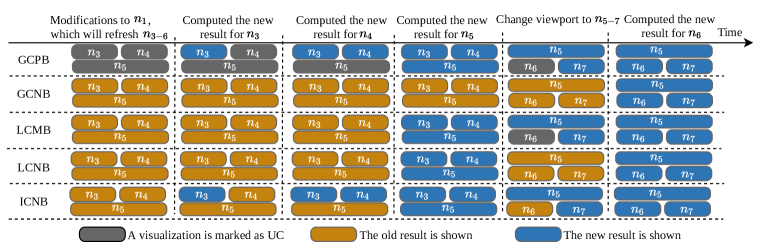
Figure 5. An example timeline for each lens presenting results to the user.

Unfortunately, with $C_{m}$, we cannot have both monotonicity and visibility: if two consecutive read transactions involve overlapping views, the latter transaction needs to read the same or more recent version of view graph compared to the former one to maintain monotonicity. Therefore, the latter transaction may read the latest graph, which may include UCs, thereby violating visibility.

Theorem 6 ($C_{m}$-impossibility).

We cannot always simultaneously maintain monotonicity, visibility, and consistency-minimal for read transactions.

Proof.

(Sketch) We construct a counterexample where the three properties cannot be met together. We assume the initial graph is $G^{t_{0}}$ and a user modifies the base table $n_{1}$ in Figure 4. This modification creates a write transaction $w^{t_{1}}$ that updates $n_{1}$ and $n_{3-6}$, and generates a new version $G^{t_{1}}$. We further assume we have computed the new results $v_{1}^{t_{1}}$ and $v_{3-5}^{t_{1}}$, but not $v_{6}^{t_{1}}$.

Based on this setup, consider two consecutive read transactions $r^{1}$ (reading $n_{3-5}$) and $r^{2}$ (reading $n_{5-7}$), which correspond to the case that the user moves the viewport. To maintain consistency-minimal, $r^{1}$ will read $G^{t_{1}}$ and return $v_{3-5}^{t_{1}}$ since $G^{t_{1}}$ does not include UCs for $r^{1}$. Now we show the subsequent transaction $r^{2}$ cannot maintain the three aforementioned properties simultaneously. To maintain monotonicity and consistency-minimal, $r^{2}$ has to read $G^{t_{1}}$. This is because both $r^{2}$ and $r^{1}$ need to read $n_{5}$, and $r^{1}$ has already read $v_{5}^{t_{1}}$ in $G^{t_{1}}$. However, reading $G^{t_{1}}$ violates visibility because $r^{2}$ needs to read $n_{6}$ but $v_{6}^{t_{1}}$ has not yet been computed for $G^{t_{1}}$. This example proves that monotonicity, visibility, and consistency-minimal cannot always be met together. ∎

Interestingly, if we sacrifice one property among the three properties, we can always maintain the other two.

Theorem 7 ($C_{m}$-possibility).

Transactional panorama can always maintain any two properties out of monotonicity, visibility, and consistency-minimal for read transactions.

Proof.

(Sketch) First, we can maintain monotonicity and visibility together for any read transaction because for each view read by this transaction, we can always return the most recent view result, without considering consistency. Second, we can also maintain visibility and consistency-minimal (or $C_{m}$). To achieve this, each read transaction reads the most recent version of view graph that has zero UCs for this transaction. Finally, we can maintain monotonicity and $C_{m}$ together because for a read transaction we could always find a version of view graph that meets monotonicity (e.g., the latest one). Among all of the versions that maintain monotonicity, we choose the one that minimizes the number of UCs for this transaction and thus achieves $C_{m}$. ∎

2.6. Property Combinations and Lenses

Given the feasible property combinations, we now define different ways of presenting results to the user while preserving a given property combination, which we call lenses. We use Figure 5 to show illustrate how each lens presents results to the user for the example in Figure 4. In this example, the base table $n_{1}$ is modified, which will refresh $n_{3-6}$, but not $n_{7}$; the viewport initially includes $n_{3-5}$ and is modified to $n_{5-7}$ after we have computed the new view results for $n_{3-5}$. Then, we discuss the lenses that are covered in existing tools and the newly discovered ones. Finally, we introduce three new variants that allow users to make better trade-offs between staleness and invisibility. For simplicity, we use $M$ for Monotonicity and $V$ for Visibility.

Lenses from Theorems 4-5. We first define the lenses derived from Theorems 4-5:

• GCNB: Globally-Consistent Non-Blocking

• GCPB: Globally-Consistent Partially-Blocking

Theorem 4 shows that it is possible to preserve $M$-$V$-$C_{c}$ together. We denote the lens for this property combination GCNB, which always reads and presents the view results from the recently committed graph to the user. On the other hand, lens GCPB preserves $M$-$C_{f}$ based on Theorem 5. It always reads the latest graph, presents new view results that are consistent with the newly modified source data, and marks a view invisible if its view result has not been computed yet. Figure 5 has shown the examples for the two lenses presenting results in the visual interface. We include “Globally Consistent (GC)” in the names of the lenses GCNB and GCPB to indicate that for these two lenses all of the results (in the viewport or otherwise) are consistent with a single version of the view graph.

Lenses from Theorems 6-7. Next, we define the lenses derived from Theorems 6-7:

• LCNB: Locally-Consistent Non-Blocking

• LCMB: Locally-Consistent Minimum-Blocking

• ICNB: Inconsistent Non-Blocking

Lens LCNB adopts $V$-$C_{m}$ from Theorem 7. Between the committed and latest view graphs, it reads the most recent version that does not have UCs for any read transaction, ensuring that each viewport does not have invisible views and that the results within a viewport are consistent. Lens LCMB adopts $M$-$C_{m}$ from Theorem 7. Between the committed and latest view graphs, it reads the most recent version that returns the minimum number of UCs for each read transaction and preserves monotonicity. Specifically, if reading either the committed or latest graph preserves monotonicity, LCMB chooses the version that has the minimum number of UCs for the read transaction, where the minimum number of UCs is zero since the committed graph includes zero UCs. Otherwise, LCMB reads the latest graph to preserve monotonicity, which may include UCs. Finally, lens ICNB preserves $M$-$V$. It allows a user to always inspect results of any views and refreshes each view independently, which sacrifices consistency. Figure 5 has shown the examples for the three lenses presenting results in the visual interface. Note that all lenses except for ICNB provide consistent results for the user (this include locally and globally consistent lenses). However, users will perceive different levels of staleness and invisibility for different lenses. In Section 2.8, we formally characterize the relative orders across lenses in terms of staleness and invisibility.

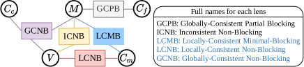
Figure 6. The possible property combinations and the corresponding base lenses covered in transactional panorama

Discovering new lenses. We call the above lenses as base lenses, and their names and corresponding properties are summarized in Figure 6. GCPB is adopted by Power BI (powerBI, ), Superset (superset, ), and Dataspread (Antifreeze, ), and ICNB is adopted by Google Sheets (sheets, ). Recall that there is an existing lens, Globally-Consistent Fully-Blocking (GCFB), that is adopted by Excel (msexcel, ), Calc (libreCalc, ), and Tableau (tableau, ). It marks all of the views invisible until the system has computed all of the new view results. We don’t consider it henceforth since it is dominated by GCPB—GCPB maintains the same properties, and has lower invisibility and equal staleness compared to GCFB. GCNB, LCNB, and LCMB are newly discovered lenses in our model.

$k$-relaxed variants. As we will show in Figure 7, the three new lenses above are optimized to achieve low invisibility, but have high staleness. Therefore, we introduce their $k$-relaxed variants to allow for more invisible views to reduce staleness such that a user can gracefully explore the performance trade-off between invisibility and staleness, as visualized in Figure 2. Specifically, $k$-GCNB, the variant of GCNB, will read the latest graph if this graph involves $k$ or fewer UCs, while GCNB reads the latest graph only when it is committed. Similarly, $k$-LCNB, corresponding to LCNB, reads the most recent version of view graph that has $k$ or fewer UCs for the read transaction, ensuring the viewport has $k$ or fewer invisible views. $k$-LCMB, the variant of LCMB, needs to maintain monotonicity and consistency, and works as follows. If reading either the committed or latest graph preserves monotonicity, $k$-LCMB reads the recent version that has $k$ or fewer UCs for the read transaction, similar to $k$-LCNB. Otherwise, $k$-LCMB reads the latest graph to preserve monotonicity.

2.7. Performance Metrics

With the different lenses defined, we now formally define the performance metrics: invisibility and staleness, for these lenses, and study their relative performance in Section 2.8.

Invisibility represents the total time when the views read by a user are invisible. We adapt the metric from previous work (Antifreeze, ) to our scenario of modeling reading the view graph as read transactions. We define $I$, the invisibility for a set of read transactions $R=\{r^{s_{1}},\cdots,r^{s_{m}}\}$, as:

$$I(R)=\sum_{i=1}^{m-1}|H_{\textsf{\small UC}}^{s_{i}}|\times(Time(r^{s_{i+1}})-Time(r^{s_{i}}))\vspace{-1.5mm}$$

$Time(r^{s_{i}})$ is the time during which $r^{s_{i}}$ returns and $H_{\textsf{\small UC}}^{s_{i}}$ is the set of UCs in the returned view states. So $|H_{\textsf{\small UC}}^{s_{i}}|\times(Time(r^{s_{i+1}})-Time(r^{s_{i}}))$ represents the time when the views read by $r^{s_{i}}$ stay invisible between two consecutive read transactions.

Staleness represents the total time during which read transactions’ returned view results are not consistent with the latest version of the view graph. We use $S$ to denote staleness for a set of read transactions $R=\{r^{s_{1}},\cdots,r^{s_{m}}\}$. Say $G^{t_{i}}$ is the latest version of the view graph before the read transaction $r^{s_{i}}$ starts, and say the returned view result by $r^{s_{i}}$ for view $n_{k}$ is $v_{k}^{t_{j}}$. $S$ is defined as:

$$S(R)=\sum_{i=1}^{m-1}\sum_{v_{k}^{t_{j}}\in H^{s_{i}}_{qr}}\mathtt{I}[v_{k}^{t_{j}}\notin V^{t_{i}}]\times(Time(r^{s_{i+1}})-Time(r^{s_{i}}))\vspace{-1.5mm}$$

Here, $H^{s_{i}}_{qr}$ represents the view results that are returned by $r^{s_{i}}$. $\mathtt{I}[v_{k}^{t_{j}}\notin V^{t_{i}}]$ is 1 if the view result is stale (i.e., $v_{k}^{t_{j}}$ does not belong to the latest version of the view graph); otherwise, it is 0. So the inner summation represents the total time when the view results returned by $r^{s_{i}}$ stay stale between two consecutive read transactions.

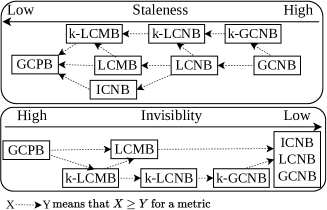
Figure 7. Summary of the orders across different lenses based on staleness and invisibility

2.8. Performance Metrics: Guarantees

We now study the trade-off between invisibility and staleness by ordering different lenses by these metrics, as is summarized in Figure 7. Recall that we already assume the system processes one write transaction at a time, so the read transactions either read the committed or latest graph. We use the acronyms for the respective lenses; the full names can be found in Figure 6. For simplicity, we use $S{(}A)$ and $I{(}A)$ to represent the staleness and invisibility for lens $A$, respectively.

We start with comparing GCPB and GCNB with other lenses. These two represent extreme points across the trade-off between staleness and invisibility since GCPB always reads the latest graph, while GCNB always reads the committed graph, and therefore sandwich other lenses.

Theorem 8.

$S{(}GCPB)\leq S{(}\text{all other lenses})\leq S{(}GCNB)$, and $I{(}GCPB)\geq I{(}\text{all other lenses})\geq I{(}GCNB)$.

Proof.

(Sketch) GCPB always reads the latest graph, so its staleness is zero and no larger than the other lenses, and its invisibility is no smaller than the other lenses (except for GCFB, which is excluded). Symmetrically, GCNB reads the latest graph only after all of the new view results are computed, so its staleness is no smaller than the other lenses, and its invisibility is no larger than the other lenses. ∎

Next, we introduce two theorems that help identify a relative ordering between LCMB, LCNB, and ICNB. Intuitively, LCMB always reads the same or more recent version than LCNB because if LCMB needs to read the latest graph to maintain monotonicity, LCNB may still read the committed graph; otherwise, both lenses read the same version of the view graph. So, LCMB has no smaller invisibility and no larger staleness than LCNB. In terms of LCNB and ICNB, ICNB reads the new view result for a view whenever it is computed, but LCNB needs to wait for all the new view results in the viewport to be computed before reading them. So, LCNB has no smaller staleness than ICNB, and they have the same zero invisibility. Finally, we find that the order between LCMB and ICNB for staleness depends on the workload, but LCMB has no smaller invisibility since LCMB may return UCs while ICNB will not.

Theorem 9.

$S{(}LCMB)\leq S{(}LCNB)$, $S{(}ICNB)\leq S{(}LCNB)$, and the order between S(LCMB) and S(ICNB) depends on the workload.

Proof.

(Sketch) We prove $S{(}LCMB)\leq S{(}LCNB)$ by showing that LCMB always reads the same or more recent version than LCNB. Specifically, we show the two cases are true: 1) if LCMB reads the committed graph, then LCNB also reads the committed graph, and 2) if LCMB reads the latest graph, LCNB may not read the latest graph. The first case is true because if LCMB reads the committed graph, it means that the latest graph includes UCs for the read transaction and LCNB also reads the committed graph. The second case is also true because when LCMB reads the latest graph, LCNB may still read the committed graph, sacrificing monotonicity in the process.

$S{(}ICNB)\leq S{(}LCNB)$ because ICNB reads the new view result for a view whenever it is computed, but LCNB needs to wait for all the new view results in the viewport to be computed before reading them. The order between $S{(}ICNB)$ and $S{(}LCMB)$ depends on the configuration of the view graph, viewport, and read/write transactions. Consider when a viewport involves multiple views to update and all of the read transactions read this viewport. In this case, LCMB has higher staleness than ICNB because ICNB can read the new result for a view whenever it is computed but LCMB needs to wait for all of the new view results in the viewport to be computed. LCMB can also have lower staleness than ICNB. Say a user first waits for the views in the viewport to be up-to-date and then proceeds to examine other views. If any two consecutive read transactions have overlapping views, then after LCMB reads the latest graph for the first viewport, it will always read the latest graph for the rest of the viewports to preserve monotonicity. In this case LCMB has high invisibility, but low staleness. ICNB, on the other hand, does not always read the view results in the latest graph after the initial viewport and can have higher staleness than LCMB. ∎

Theorem 10.

$I{(}LCMB)\geq I{(}LCNB)=I{(}ICNB)$ for invisibility.

Proof.

(Sketch) LCNB and ICNB have the same zero invisibility since they are non-blocking. LCMB has larger or equal invisibility compared to LCNB and ICNB because LCMB may return UCs and does not always have zero invisibility. ∎

Our final two theorems order each $k$-relaxed variant and their corresponding base lens, and the three $k$-relaxed variants relative to each other. Intuitively, a $k$-relaxed variant always reads the same or more recent version than the corresponding base lens due to the $k$ additional UCs allowed, so it has no greater staleness and no smaller invisibility than the corresponding base lens. In addition, the ordering across $k$-relaxed variants is the same as their corresponding base lenses since they allow the same number of UCs.

Theorem 11.

A $k$-relaxed variant has no greater staleness and no smaller invisibility than the corresponding base lens.

Proof.

(Sketch) The $k$-relaxed variant always reads the same or more recent version than the corresponding base lens due to the $k$ additional UCs allowed, and thus has no larger staleness and no smaller invisibility than the corresponding base lens. ∎

Theorem 12.

$S{(}$k$-LCMB)\leq S{(}$k$-LCNB)\leq S{(}$k$-GCNB)$ and $I{(}$k$-LCMB)\geq I{(}$k$-LCNB)\geq I{(}$k$-GCNB)$.

Proof.

(Sketch) To compare $k$-LCMB and $k$-LCNB, we show that $k$-LCMB will consistently read the same or more recent version of the view graph than $k$-LCNB. Specifically, if $k$-LCMB reads the committed graph, it means the latest graph includes more than $k$ UCs for the viewport, so $k$-LCNB also reads the committed graph by definition. In addition, if $k$-LCMB reads the latest graph, $k$-LCNB may read the committed graph because $k$-LCNB does not need to preserve monotonicity. So we have $S{(}$k$-LCMB)\leq S{(}$k$-LCNB)$ and $I{(}$k$-LCMB)\geq I{(}$k$-LCNB)$. In terms of $k$-LCNB and $k$-GCNB, $k$-LCNB reads the latest graph when this graph has $k$ or fewer UCs for the read transaction, but $k$-GCNB can read the latest graph only when the latest graph has $k$ or fewer UCs overall. So we have $S{(}$k$-LCNB)\leq S{(}$k$-GCNB)$ and $I{(}$k$-LCNB)\geq I{(}$k$-GCNB)$. ∎

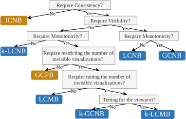
Figure 8. Selection of the appropriate lenses

2.9. Selecting Appropriate Lenses

We’ve introduced a number of lenses so far, many of which do not strictly dominate each other. Selecting the right lens depends on user needs and use cases. We now provide guidance for selecting the appropriate lens, summarized as a decision tree in Figure 8, where the existing lenses are marked as gold boxes and the new lenses are marked as blue. If the user does not require consistency across multiple visualizations, ICNB is the best choice since it maintains both monotonicity and visibility, and has low staleness. Otherwise, we check whether visibility is required. If yes, we choose between LCNB and GCNB, depending on the whether the user wants to additionally maintain monotonicity. If visibility is not required, we additionally check whether monotonicity is required. If not, we use $k$-LCNB to reduce staleness and invisibility. Note that $k$-LCNB subsumes LCNB. If the user does not want to tune the $k$ value, they can adopt LCNB. On the other hand, if monotonicity is needed, we check whether the user needs to restrict the number of invisible visualizations in the dashboard. If not, which means the user wants to see the new view results without worrying about invisibility, then GCPB is adopted. Otherwise, we further check whether the user wants to tune the $k$ value. If not, LCMB is adopted. If yes, $k$-GCNB or $k$-LCMB is adopted depending on whether the user wants to tune the $k$ value with respect to the viewport or the dashboard overall.

2.10. Extensions

We now discuss extending our transactional panorama model to support reading and modifying the definition of a view graph, and user actions beyond modifying the location of the viewport ,concurrent write transactions, and multiple users, and various UI designs.

Supporting reading and modifying view definitions. We now consider the settings where the user can read and modify view definitions. The user can read a view definition if it is rendered alongside the corresponding visualization in the viewport. Here, a read transaction is extended to read view results and/or view definitions in the viewport, depending on which of them are rendered. To support modifying a view definition, the view graph’s edges and view definitions are multi-versioned; that is, a version of view graph is defined to be $G^{t_{i}}=(E^{t_{i}},N^{t_{i}},V^{t_{i}})$. A modification to a view definition is modeled as a write transaction that modifies the view definition and refreshes the visualizations that depend on it (e.g., modifying a filter on a base table will refresh the visualizations derived from this base table). The system and scheduler processes such a write transaction in the same way as they process the write transaction stemming from modifying the source data.

Supporting user actions beyond modifying the viewport. In addition to moving the viewport, the user can also modify the visualizations in a dashbaord, by filtering, panning and shifting, brushing and linking, and drilling down/up/across charts. We break such actions into two broad categories. If the user action needs to be processed at the back-end (e.g., a web server), where transactional panorama operates, then this action is interpreted as a write transaction that involves modifying the view definition (e.g., modifying a filter). Otherwise, if the user action is performed at the front-end (e.g., shifting a visualization), transactional panorama does not need to intervene.

All that said, while supporting the aforementioned actions, the visual interface may present the old view definition for some lenses even after the user modifies the view definition (e.g., presenting the old value of a filter after it is modified for GCNB to preserve consistency), which introduces additional complications regarding the desired user experience. If, for example, the dashboard designer determines that the dashboard should not show an old filter value to the user after they have updated it — since that might be confusing to the user, then the selected lens can be overridden to be either GCPB or ICNB to process the case for modifying and reading a filter. For all other cases, the selected lens will be used.

Supporting concurrent write transactions. We also support concurrent write transactions in a single user setting, which means a user or an external system can submit a write transaction while the previous one is not finished. Here, each new write transaction creates a new version of view graph as discussed in Section 2.3 and write transactions are committed with respect to the order they are submitted. The definitions of MVC properties for read transactions do not change in this scenario. For example, for consistency-minimal, a read transaction returns the results of the version that has the minimal UCs for this transaction.

Supporting multiple users. transactional panorama can be easily extended to support multiple users reading the same dashboard. Here, each user can choose different MVC properties and we process each user’s read transactions based on the selected properties separately. We leave the case of supporting concurrent writes from multiple users to future work.

UI designs. Instantiating transactional panorama requires new UI designs in the dashboard, such as helping the user identify the version of view graph they are looking at and effectively demonstrate the multiple choices of lenses to the user in the dashboard. For example, to differentiate two versions (for the case of processing one write transaction at a time), we can annotate the visualization that belongs to the committed graph and requires to be updated with a special indicator, such as a progress bar on the side. Prior work also studies UI designs for differentiating multiple versions (WuCH020InteractionSnapshots, ), which can be leveraged in transactional panorama if multiple concurrent write transactions exist. However, the UI designs are not the focus of this paper and left for future work.

3. Maintaining MVC properties

We now discuss how to maintain different property combinations for different lenses defined in transactional panorama. Specifically, we discuss the design of the view graph and auxiliary data structures (Section 3.1), and the algorithms for maintaining MVC properties separately (Section 3.2-3.3) and maintaining property combinations for each lens (Section 3.4). We assume a ReadTxn manager responsible for processing read transactions, and another WriteTxn manager responsible for processing write transactions. The ReadTxn and WriteTxn managers are assumed to run on separate threads to enable concurrent execution of the two types of transactions. In Section 5, we discuss the strategy for triggering write transactions.

3.1. View Graph and Auxiliary Data Structures

We maintain a multi-versioned view graph. Each node stores a list of items, called item list, where a item could be a view result or UC, and created by a new write transaction. Recall that a UC is a place-holder for the corresponding view result. Each node in the view graph is associated with a latch to synchronize concurrent reads/writes to its item list.

We additionally maintain an auxiliary table, MetaInfo, to store the timestamps of the last committed and latest view graphs (denoted as $t_{c}$ and $t_{s}$, respectively), and the number of UCs for the latest graph (denoted as $c_{\textsf{\small uc}}$). The quantities $t_{c}$, $t_{s}$, and $c_{\textsf{\small uc}}$ are maintained by the WriteTxn manager and will be used by the ReadTxn manager to preserve the properties specified by the user. We also include a latch to synchronize concurrent accesses to the MetaInfo table, which means any access to MetaInfo needs to acquire this latch.

3.2. Maintaining Consistency

We now discuss preserving three types of consistency: $C_{c}$, $C_{f}$, and $C_{m}$, and will discuss preserving monotonicity and visibility separately in the next subsection. Intuitively, maintaining consistency for a read transaction means this transaction can read the recently committed and latest view graphs. However, traditional concurrency control protocols, such as 2PL or OCC (BernsteinHG87CCBook, ), do not apply here because they do not support the type of consistency that reads an uncommitted version of the view graph (i.e., $C_{f}$ and $C_{m}$). To maintain consistency, we process a read transaction in two steps:

1. Atomically find the timestamps for the last committed and latest view graphs (i.e., $t_{c}$ and $t_{s}$ in MetaInfo)

2. Read the versions of view graph for $t_{c}$ and $t_{s}$.

Step 1) is done correctly via the latch on the MetaInfo table. Step 2) requires that the view graphs for $t_{c}$ and $t_{s}$ exist, which is done by the WriteTxn manager. Step 2) additionally requires an algorithm for reading a version of view graph for given a timestamp, which is done in the ReadTxn manager. We now discuss the designs of ReadTxn and WriteTxn managers for maintaining consistency.

WriteTxn manager. The WriteTxn manager processes a write transaction $w^{t_{i}}$ in three steps:

1. Create a new version of view graph for $w^{t_{i}}$

2. Compute the view results for the views involved in $w^{t_{i}}$ and update the view graph with the new results

3. Update $t_{c}$ with $t_{i}$

Step 1) guarantees that the timestamp of the latest view graph, $t_{s}$, exists. Specifically, the WriteTxn manager creates a new version of view graph by appending UCs to the item lists of the nodes that $w^{t_{i}}$ needs to update. Then it atomically updates $t_{s}$ with the timestamp of the running write transaction $w^{t_{i}}$, and $c_{\textsf{\small uc}}$, the number of UCs for the latest graph, in MetaInfo. Step 2) computes the view result and replaces the corresponding UC for each view, and updates $c_{\textsf{\small uc}}$. It leverages a scheduler to decide the order of computing the view results to reduce invisibility and/or staleness, which we discuss in Section 4. Step 3) updates the timestamp of the last committed version (i.e., $t_{c}$) with $t_{i}$, which guarantees that the version of view graph for $t_{c}$ exists. We say $w^{t_{i}}$ is committed if we have successfully performed the aforementioned three steps for $w^{t_{i}}$.

ReadTxn manager. The ReadTxn manager uses timestamps $t_{c}$ and $t_{s}$ to read the last committed and latest view graphs. Depending on the properties that need to be maintained, the ReadTxn manager decides the version to read, which is discussed in Section 3.4. Here, we present the algorithm for reading a version of view graph. Assuming a transaction $r^{s_{j}}$ needs to read $G^{t_{i}}$, the intuition is that for each view read by $r^{s_{j}}$, we read the recent view result/UC whose timestamp is no larger than $t_{i}$. The reason is that we have two possible cases if a view result/UC for a node $n_{k}$ belongs to $G^{t_{i}}$: 1) $n_{k}$ is or will be modified by $w^{t_{i}}$, in which case we have a view result/UC whose timestamp is $t_{i}$; 2) $n_{k}$ is not modified by $w^{t_{i}}$, in which case the most recent view result whose timestamp is smaller than $t_{i}$ belongs to $G^{t_{i}}$.

3.3. Maintaining Monotonicity and Visibility

To guarantee monotonicity, in the ReadTxn manager we maintain a table (denoted as LastRead) that stores the timestamps of the view results or UCs that are last read. Monotonicity requires that a read transaction reads the view results or UCs whose timestamps are no smaller than the corresponding timestamps in the LastRead table. To maintain visibility, we guarantee that the view states returned by a read transaction do not include UCs.

3.4. Maintaining Property Combinations

For the lenses that need to maintain consistency, we read the MetaInfo and LastRead table to decide which versions of the view graph to read. Specifically, to maintain $M$-$C_{f}$ for GCPB we use $t_{s}$ in MetaInfo to read the latest graph. Similarly, to preserve $M$-$V$-$C_{c}$ for GCNB, we use $t_{c}$ to read the last committed graph. For $k$-GCNB, we need to check whether the number of UCs for the latest graph (i.e., $c_{\textsf{\small uc}}$ in MetaInfo) is no larger than $k$. If so, we read the version for $t_{s}$, otherwise, $t_{c}$ is used.

Maintaining $V$-$C_{m}$ for LCNB will read both the last committed and latest view graphs. Among the two sets of returned view states, we choose to return the set that does not have UCs and corresponds to the more recent version. Maintaining $M$-$C_{m}$ for LCMB requires preserving monotonicity. This is done by checking the LastRead table to see whether reading the committed version violates monotonicity. If not, LCMB follows the same procedure of LCNB. Otherwise, LCMB will read the latest graph. $k$-LCNB and $k$-LCMB are processed similarly with $k$ UCs relaxed.

For the property combination $M$-$V$ (adopted by ICNB), which sacrifices consistency, we do not need to read MetaInfo. Instead, we directly read the view graph and return the most recent view result for each node involved in the read transaction.

4. write transaction Scheduler

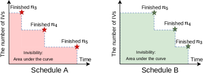
Figure 9. The impact of different schedules on invisibility

As mentioned in Section 3, the scheduler, which decides the order of computing the new view results for a write transaction, impacts invisibility and staleness for all lenses except GCNB. GCNB will only read the latest graph after all of the views are updated, so its staleness and invisibility are independent of the scheduler. We analyze two factors that impact the performance of the scheduler and design a scheduling algorithm that considers these factors to reduce invisibility and staleness. Our discussion assumes processing a write transaction $w^{t_{i}}$ that updates a set of nodes $N_{w}^{t_{i}}$.

Factors that impact invisibility and staleness. Staleness (or invisibility) is increased if a view that is read by a user is stale (or invisible), respectively. Therefore, prioritizing computing new results for views that a user will spend more time reading will best reduce the values of the two metrics. Since it is impossible to exactly predict how long the user will spend reading a view, we use $D_{k}^{t_{i}}$, the total time during which a view $n_{k}$ has been read in the viewport since the write transaction $w^{t_{i}}$ started as a proxy. Using $D_{k}^{t_{i}}$ is based on the assumption that the user will spend more time on a view in the future if they spent more time on this view in the past. However, as this assumption weakens, $D_{k}^{t_{i}}$ will be less effective in reducing invisibility and staleness, as we will see in Section 6.3. For a set of read transactions $R=\{r^{s_{1}},\cdots,r^{s_{m}}\}$ after $w^{t_{i}}$ is started, $D_{k}^{t_{i}}$ is defined as

$$D_{k}^{t_{i}}=\sum_{j=1}^{m-1}\mathtt{I}[n_{k}\text{ is read by }r^{s_{j}}]\times(Time^{\prime}(r^{s_{j+1}})-Time^{\prime}(r^{s_{j}}))$$

$Time^{\prime}(r^{s_{j}})$ is the time when the system receives the read transaction $r^{s_{j}}$. $\mathtt{I}[n_{k}\text{ is read by }r^{s_{j}}]$ is 1 if the view $n_{k}$ is in the viewport when $r^{s_{j}}$ is issued, otherwise 0. Therefore, $\mathtt{I}[n_{k}\text{ is read by }r^{s_{j}}]\times(Time^{\prime}(r^{s_{j+1}})-Time^{\prime}(r^{s_{j}}))$ represents the duration when the view $n_{k}$ stays in the viewport between two consecutive read transactions. The system tracks the arrival time of each read transaction and the views that are read by this transaction to calculate $D_{k}^{t_{i}}$. In our scheduling algorithm, we prioritize scheduling the view that has higher $D_{k}^{t_{i}}$.

In addition, there is another factor that impacts the staleness and invisibility: the different amounts of time for computing the results for different views. Intuitively, prioritizing computing the new result for the view that has the least execution time will allow the user to read a fresh view earlier, which is also observed by previous work (Antifreeze, ). We use an example to illustrate this. Here, say the write transaction $w^{t_{i}}$ updates the base table $n_{1}$ and $n_{3-6}$ in Figure 4, the views $n_{3-5}$ are in the current viewport, and the viewport does not change. We additionally assume we need to maintain properties $M$-$C_{f}$ (i.e., always reading the last created version) and want to minimize invisibility. Figure 9 shows two different schedules for $n_{3-5}$, where the x-axis plots the execution time while the y-axis plots the number of UCs. The invisibility is essentially the area under the curve: the sum of the times of each view being invisible. We see that while both schedules have the same execution time, Schedule A has lower invisibility than Schedule B because it always prioritizes computing the view result that has the least execution time. This heuristic can similarly reduce staleness for other property combinations (e.g., $M$-$C_{m}$). We use $Q_{k}^{t_{i}}$ to represent the amount of time for computing the new result for the view $n_{k}$ while processing $w^{t_{i}}$. The view that has a smaller $Q_{k}^{t_{i}}$ should have a higher priority.

1 $N_{w}^{t_{i}}\leftarrow$ Topologically sort $N_{w}^{t_{i}}$

2 O $\leftarrow$ Break $N_{w}^{t_{i}}$ into topologically independent groups

3 for $O^{l}\in O$ do

4       while $O^{l}$ is not empty do

5             $n_{max}\leftarrow\displaystyle\operatorname*{arg\,max}_{n_{k}\in O_{l}}\leavevmode\nobreak\ P_{k}^{t_{i}}=\frac{D_{k}^{t_{i}}}{Q_{k}^{t_{i}}}$

6             Update the view $n_{max}$

7             $O^{l}\leftarrow O^{l}\backslash\{n_{max}\}$

8            

9       end while

10      

11 end for

Algorithm 1 Scheduling algorithm in the WriteTxn manager

Scheduling algorithm. We design a metric $P_{k}^{t_{i}}=D_{k}^{t_{i}}/Q_{k}^{t_{i}}$ to decide the priority of a view $n_{k}$. $P_{k}^{t_{i}}$ captures the characteristics of the two aforementioned factors. If two views have the same $D_{k}^{t_{i}}$, a lower $Q_{k}^{t_{i}}$ yields a higher $P_{k}^{t_{i}}$. Similarly, for the same $Q_{k}^{t_{i}}$, a higher $D_{k}^{t_{i}}$ results in a higher $P_{k}^{t_{i}}$.

Algorithm 1 shows the scheduling algorithm. We first sort $N_{w}^{t_{i}}$, the set of nodes $w^{t_{i}}$ will update, topologically, break them into topologically independent groups, and compute each group with respect to the topological order. That is, we should only compute view results for views whose precedents are updated. To schedule a view to be updated within a group, we compute $P_{k}^{t_{i}}$ for each yet computed view $n_{k}$ in this group and choose the view with the highest $P_{k}^{t_{i}}$.

5. Prototype Implementation

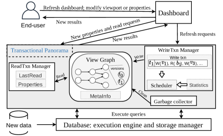
Figure 10. Overview of our implementation in Superset

We now discuss implementing the transactional panorama framework in Superset (superset, ), a widely used open-source BI toolthat has 47.3k stars on Github and similar functionality to Tableau (tableau, ) and PowerBI (powerBI, ). Superset provides a web-based client interface, where a user can define visualizations and organize them as part of a dashboard. Superset adopts a web server to process front-end requests and employs a database to store the base tables and compute new view results for visualizations.

Figure 10 shows an overview of the system. The user interacts with a dashboard by changing the viewport to explore different subsets of visualizations, selecting desired properties, and refreshing the dashboard with respect to changes to the underlying data. As in today’s many BI tools, the dashboard can be refreshed manually or configured to refresh periodically (e.g., every 1 min). When the dashboard needs to be refreshed, it sends a refresh request to the WriteTxn manager, where each refresh request is interpreted as a write transaction. After a refresh request is sent, the dashboard will regularly send read requests to the ReadTxn manager to pull refreshed visualizations. Each read request includes the viewport information, which is leveraged by the ReadTxn manager to construct read transactions. When the system has finished the write transaction, the ReadTxn manager returns the new view results that have not yet been read by the user to the dashboard to refresh all of its visualizations, after which, the dashboard stops sending new read requests. When the system is not processing a write transaction, the user can change the desired properties. Changing the properties on the fly is left for future work.

We store the base tables in the database and maintain the results of the derived visualizations along with the view graph in memory in the web server. We also include a garbage collector to clean up view results in the view graph that are guaranteed to not be read in the future. To safely clean up the useless view results, we maintain a timestamp, $t_{r}$, representing the oldest version of view graph that a read transaction is reading or will read in the future. With $t_{r}$, the garbage collector can safely remove the view results that belong to the older versions of view graph than $t_{r}$. We maintain $t_{r}$ by updating it with $t_{c}$, the timestamp for most recently committed version of view graph, before each read transaction starts, because the oldest possible version a read transaction will read is the committed graph.

6. Experiments

The high-level goal of our experiments is to characterize the relative benefits of different lenses for various workloads—to help users select the right lens for their needs and make appropriate performance trade-offs (Section 6.1). Our experiments also seek to demonstrate the value of the new lenses, which provide new trade-off points for the user to select (Section 6.1-6.2), and evaluate the performance benefit and overhead of the optimizations for the write transaction scheduler (Section 6.3). Our experiments address the following research questions:

1. [Workload impact on performance] How do different user behaviors and dashboard configurations impact invisibility and staleness for the base lenses in transactional panorama? (Section 6.1)

2. [Performance benefit of new lenses] How much do the new lenses reduce invisibility while maintaining consistency, compared to existing lenses? (Section 6.1)

3. [Trade-offs provided by $k$-relaxed variants] How do different $k$ values impact the invisibility and staleness for the $k$-relaxed variants? (Section 6.2)

4. [Impact of optimized scheduling] How much does our write transaction scheduler decrease or increase invisibility and staleness? (Section 6.3)

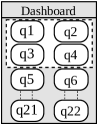
Figure 11. TPC-H dashboard

Configurations	Options	Default Value
Read behavior	{Regular Move, Wait and Move, Random Move }	Regular Move
Explore range	{22, 16, 10, 4}	22
Viewport size	{4, 10, 16, 22}	4

Table 3. Experiment configurations

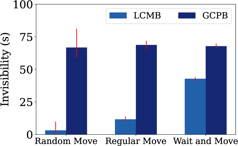
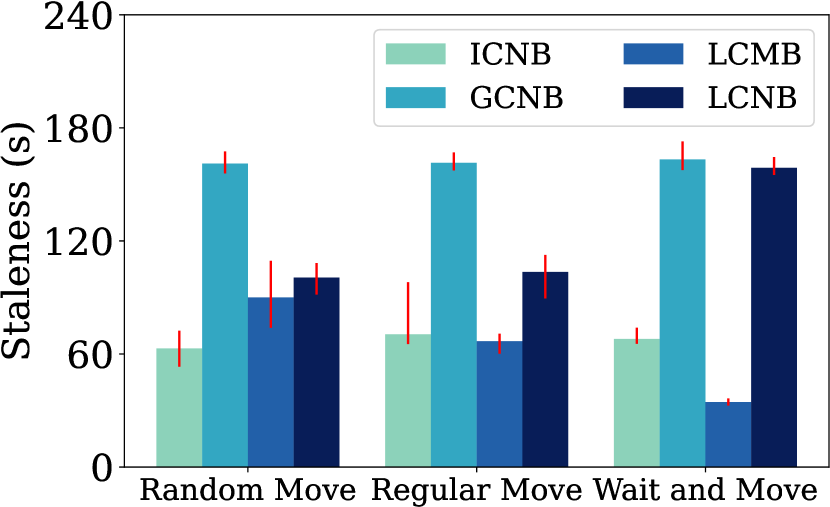
(a) Invisibility (b) Staleness

Figure 12. Evaluations of different read behaviors

Figure 13. Performance trade-off for Regular Move (a) Invisibility (b) Staleness Figure 14. The number of invisible and stale views in the viewport during the refresh

Benchmark. We build a dashboard based on the TPC-H benchmark. This dashboard includes 22 visualizations for all of the 22 TPC-H queries and runs on 1 GB of data stored in PostgreSQL. This dashboard places two visualizations in a row, as in Figure 11. We test one refresh of the dashboard with respect to modifications to the base tables unless otherwise specified, since the main focus of this paper is on the scenario where there is only one write transaction in the system at a time. This case happens when the period for triggering a refresh is longer than the time for executing the refresh, or if the system only processes one refresh at a time. For the test of one refresh, we insert 0.1% new data to the tables Lineitem, Orders, and PartSupp and then refresh all of the 22 visualizations. One test ends when we have computed the new view results for all visualizations.

We build a test client to simulate different user behaviors and dashboard configurations. Similar to the web client of Superset, this client sends web requests to the web server to trigger a refresh (i.e., start a write transaction), configure the lens used for processing a refresh, and regularly pull refreshed results of visualizations in the viewport (i.e., start read transactions). We simulate three types of user behaviors in moving the viewport to read different visualizations, which we call the read behavior: 1) Regular Move: regularly moving the viewport downward or upward and reversing the direction if we reach the boundary of the dashboard; 2) Wait and Move: similar to the first one with the difference that it only moves the viewport after all of visualizations in the viewport are refreshed; and 3) Random Move: randomly chooses a viewport, which simulates the behavior where the user moves around a lot in the dashboard. For the three behaviors, the viewport is placed at the top of the dashboard at the beginning of each test and moved every 1 second. For the first two behaviors, each move changes the viewport by a row of visualizations. The test client can additionally vary the number of visualizations the user will inspect in the dashboard (denoted as explore range) during a test. We assume these visualizations are at the top of the dashboard. For example, explore range 4 means that the user will explore the visualizations for $q_{1-4}$ in Figure 11 during a refresh. Our experiments also vary the number of visualizations in the viewport (denoted as viewport size) to evaluate how the relative sizes of the viewport and the dashboard impact invisibility and staleness. The experiment configurations are summarized in Table 3 and we use default configurations unless otherwise specified.

Configurations, and measuring invisibility and staleness. The experiments are run on a t3.2xlarge instance of AWS EC2, which has 16 GB of memory and 8 vCPUs, and uses Ubuntu 20.04 as the OS. Our experiments use PostgreSQL 10.5 with default configurations. The time interval between two consecutive read transactions is set to be 100 ms to avoid overwhelming the web server. that is, the test client sends requests to pull refreshed results every 100 ms. We run each test three times and report the mean number except for the tests that involve Random Move. For those tests, we run each 10 times and report the min, max, and mean.

To measure invisibility and staleness, the test client tracks the timestamp when each read transaction returns and the content of the returned view states, which include information for whether each returned view state is a UC or a stale view result. Using this information and the definitions in Section 2.7, we can compute invisibility and staleness. For example, the invisibility for one test is initialized to 0. During the test, if a read transaction has returned a UC for a view, then the time difference between when this and the next read transaction return will be added to the invisibility.

6.1. Performance of Base Lenses

Takeaways: 1) The new lenses significantly reduce invisibility while preserving consistency, compared to the existing lens GCPB; 2) A larger explore range increases the invisibility and staleness for all lenses except GCNB; 3) The staleness of all lenses except GCPB increases with a larger viewport size and converges to GCNB when the viewport size equals the dashboard size.

We evaluate the configurations in Table 3 for the base lenses using one refresh. Afterwards, we test the impact of varied refresh intervals for multiple refreshes.

Read behavior. Figure 12 reports the invisibility and staleness for the base lenses under different read behaviors. Each test reports the mean with the min/max as the error bar (i.e., the red line). We note that if the invisibility or staleness for a lens is zero, then that lens is not shown in the figure. To better see the trade-off between invisibility and staleness, we also plot the two metrics together in Figure 14 for Regular Move. We observe significant differences in invisibility and staleness for different lenses in Figure 12—the new lenses (i.e., LCMB, LCNB, and GCNB) can significantly reduce invisibility while maintaining consistency compared to the existing lens GCPB. Specifically, GCPB has the highest invisibility because it always reads the latest graph, and LCMB, the lens that first reads the committed graph and switches to read the latest graph, can reduce invisibility by up to 95.2% compared to GCPB (i.e., Random Move). LCMB reduces less invisibility in the case of Wait and Move because it spends a longer time on reading the latest graph. That is, after the first viewport, LCMB always reads the latest graph for the rest of the viewports due to the overlapping views across consecutive viewports. LCNB and GCNB have zero invisibility. Recall that LCNB always reads the version of view graph with zero UCs for the viewport to maintain consistency and visibility, but sacrifices monotonicity, and GCNB reads the last committed graph until all of the new view results are computed for the latest graph. ICNB also has zero invisibility, but sacrifices consistency.

On the other hand LCMB, LCNB, and ICNB can significantly reduce staleness relative to GCNB. For example, LCMB reduces staleness by up to 78.9% compared to GCNB (i.e., for Wait and Move). LCMB reduces the staleness by sacrificing visibility while ICNB and LCNB need to sacrifices consistency and monotonicity, respectively. Overall, these results show that it is valuable to enable a user to have these options to make appropriate trade-offs. In addition, Figure 12 verifies the result that the order between ICNB and LCMB for staleness is undecided in Section 2.8—the staleness of ICNB can be either higher or lower than LCMB in Figure 12.

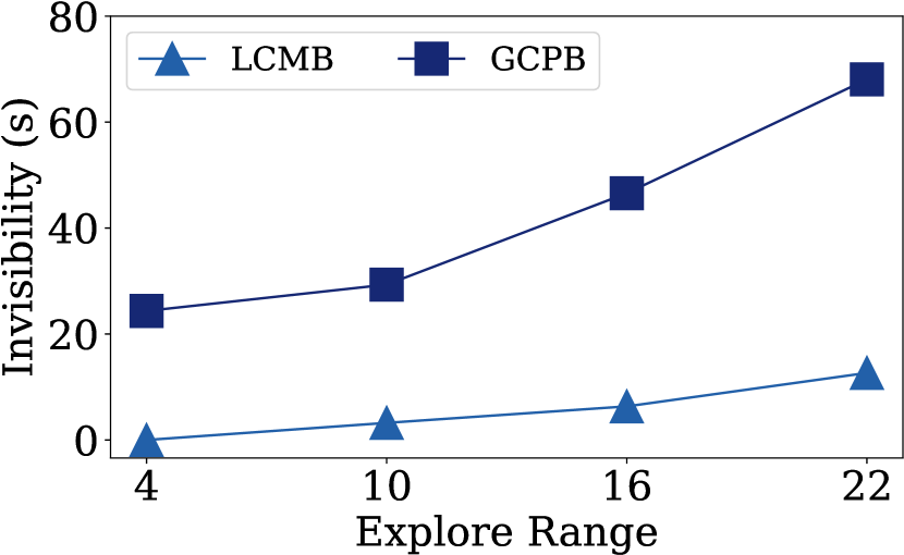
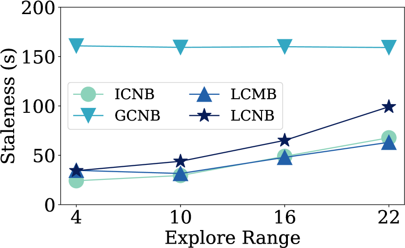
(a) Invisibility (b) Staleness

Figure 15. Evaluations of different explore ranges

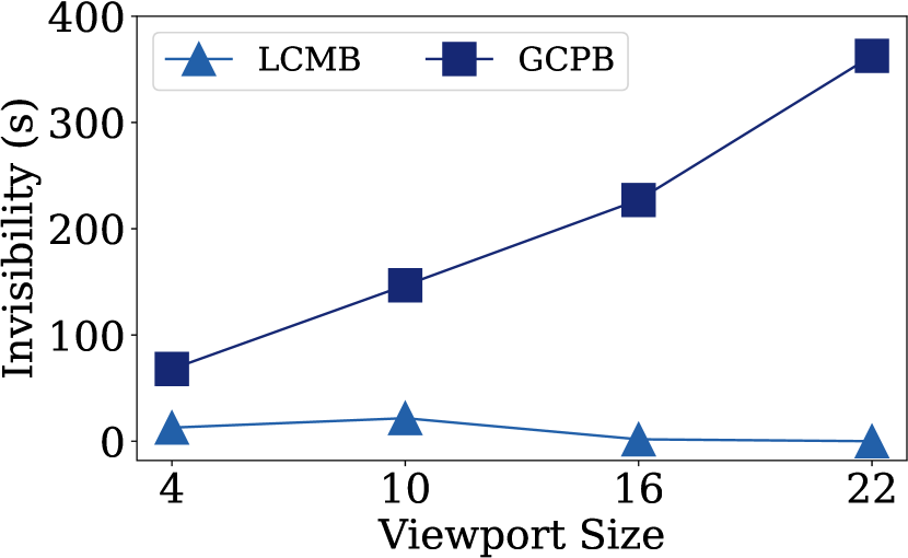
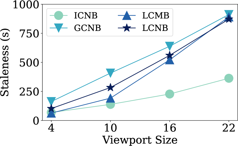
(a) Invisibility (b) Staleness

Figure 16. Evaluations of different viewport sizes

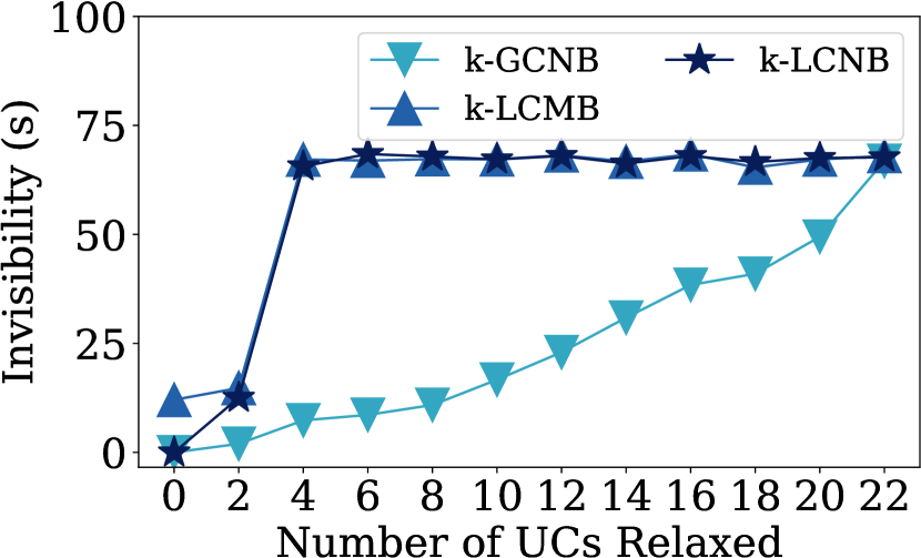
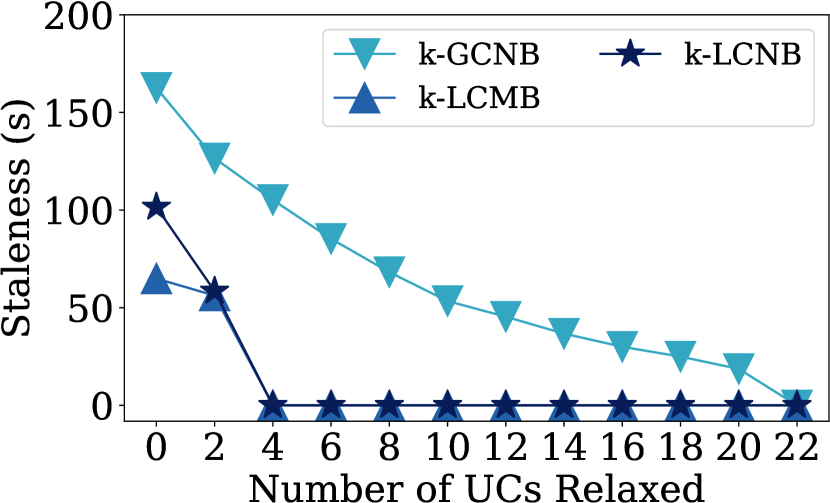
(a) Invisibility (b) Staleness

Figure 17. Evaluations of varied $k$ values

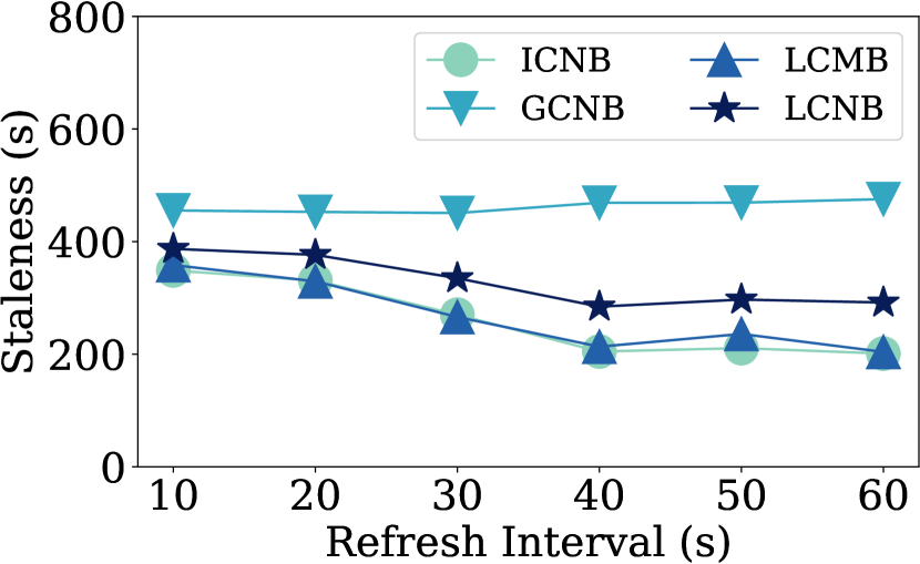
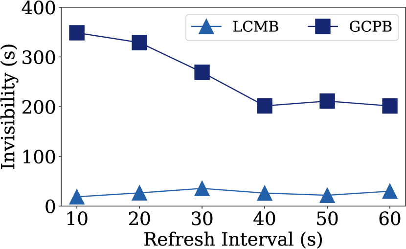
(a) Staleness (b) Invisibility

Figure 18. Evaluation of varied refresh intervals

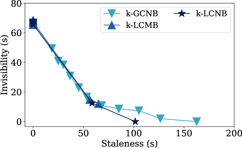
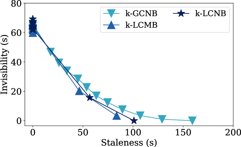
(a) Regular Move (b) Random Move (c) Wait and Move

Figure 19. Trade-off between invisibility and staleness with varied $k$ values

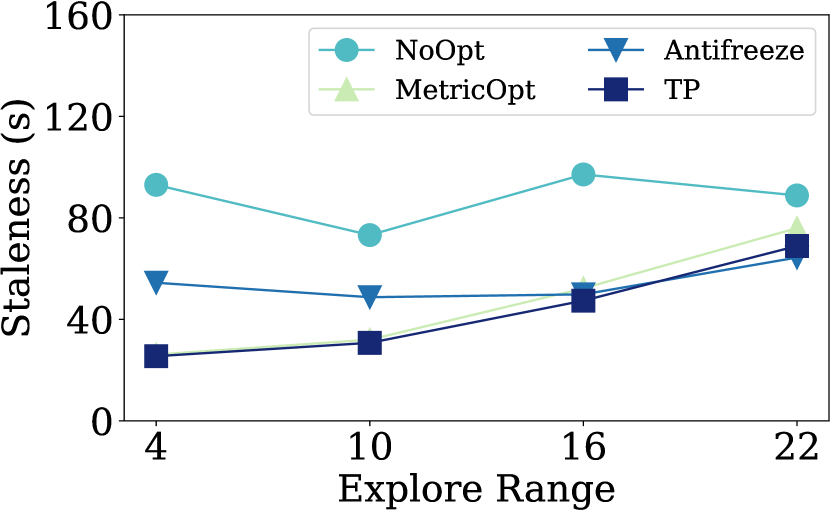
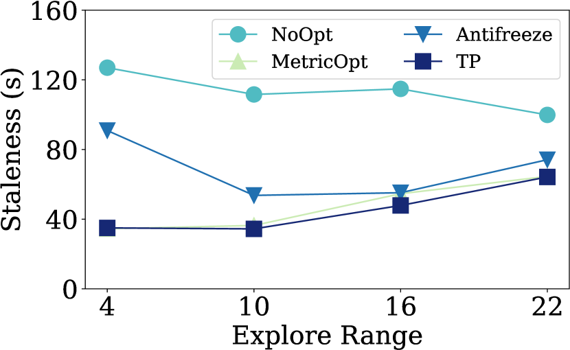
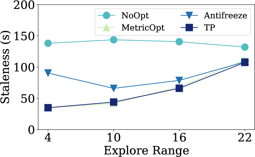
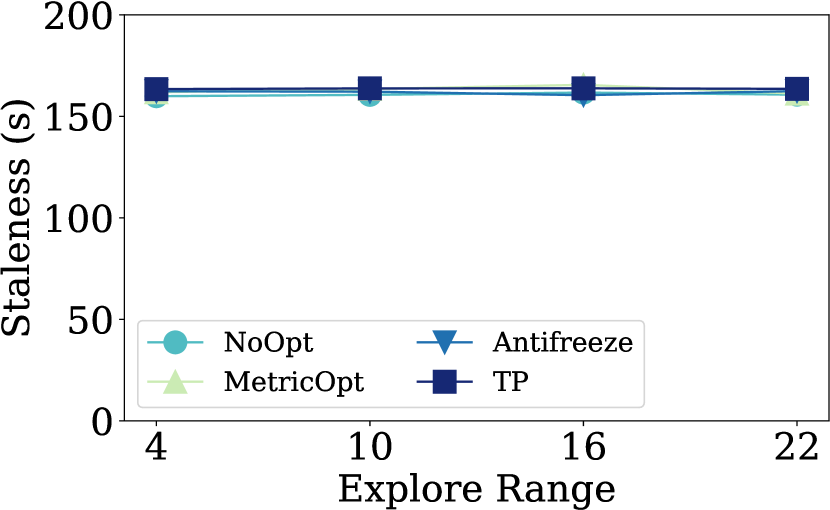
(a) ICNB (b) LCMB (c) LCNB (d) GCNB

Figure 20. Evaluation of scheduler optimizations (staleness)

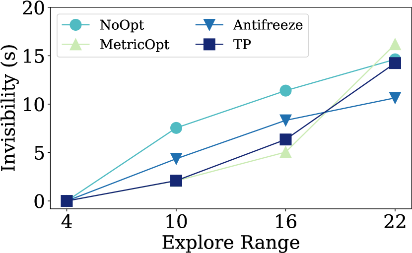
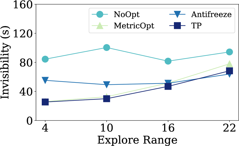
(a) LCMB (b) GCPB

Figure 21. Evaluation of scheduler optimizations (invisibility)

To better understand the behavior of different lenses, we further report the returned number of invisible and stale views by read transactions for Regular Move while we are processing the write transaction. We aggregate the read transactions that finish for every 2s and report the mean in Figure 14. The areas under the curve represent the invisibility/staleness in the respective figures. In Figure 14, GCPB initially returns many UCs as it reads the new version, and the number of UCs decreases as we compute more view results. Specifically, for the first 10s, a user sees more than 3 UCs on average, out of the 4 visualizations in the viewport. Therefore, this user cannot interact for the first 10s, significantly diminishing interactivity. LCMB, on the other hand, initially reads the committed graph to avoid invisible views. Then, it reads the latest graph (i.e., after 15s) to present fresh results to the user as GCPB does. Figure 14 shows the number of stale views over time. GCNB reads the same number of stale views as the viewport size (i.e., 4 in our test) until the last transaction. LCMB, LCNB, and ICNB can read the new version during refresh, which reduces staleness.

Explore range. This experiment evaluates the impact of varied explore ranges on different lenses. The results in Figure 15 show that we have smaller invisibility/staleness for GCPB, LCMB, LCNB, and ICNB when the user explores a smaller number of visualizations because these lenses are more likely to read the new results for smaller explore ranges. The staleness for GCNB is independent of the value of explore range since it only refreshes the visualizations after all of the view results for the new version are computed.

Viewport size. Figure 16 reports the results of varying the viewport sizes. The invisibility for GCPB increases as viewport size increases because the user will read more invisible views for each read transaction. However, the invisibility for LCMB slightly increases and then decreases to zero. The reason for decreasing invisibility is that a larger viewport size pushes LCMB to wait longer to read the latest graph, which decreases invisibility. In an extreme case, when the viewport size covers the whole dashboard, LCMB’s performance converges to GCNB, which has zero invisibility but the highest staleness, as shown in Figure 16. The staleness for GCNB, LCMB, LCNB, and ICNB increases as they will read more stale views in one read transaction. Overall, when the user explores more visualizations, the difference on invisibility and staleness will become more significant across different lenses.

Refresh interval. We test three refreshes triggered periodically, where the interval between two succeeding refreshes (i.e., refresh interval) is varied from 10s to 60s. Same as the test for one refresh, before starting each refresh, we insert 0.1% new data to the database. We report the staleness and invisibility for different lenses. Figure 18 shows that a smaller refresh interval introduces higher staleness and invisibility when the refresh interval is less than the execution time for processing a refresh (i.e., 37s in our test) for all lenses except GCNB. This is because while a version of the view graph is being computed, a smaller refresh interval creates a new version of the view graph earlier. This leads the view results of the under-computation version of the view graph to become stale earlier, and, in turn the staleness and invisibility are increased. The staleness of GCNB is not impacted by the varied refresh interval because GCNB presents the up-to-date view results to the user when it finishes all of the refreshes in the system and its staleness is determined by the execution time for finishing multiple refreshes, which is independent of the refresh interval.

6.2. Performance of $K$-Relaxed Variants

Takeaway: The $k$-relaxed variants allow the user to gracefully explore the trade-off between invisibility and staleness, and enable more trade-off points that are not covered in base lenses.

We evaluate the impact of $k$ for the $k$-relaxed variants; Recall that $k$ represents the additional $\textsf{\small UC}{s}$ permitted while reading the latest graph for LCMB, LCNB, and GCNB. Here, we vary the $k$ from 0 to 22 with an interval of 2. Our results in Figure 17-19 show that the $k$-relaxed variants gracefully explore the trade-off between invisibility and staleness, and enable more trade-off points that are not covered in base lenses. Figure 17 shows that as we admit more UCs, the invisibility increases for the $k$-relaxed variants. However, when $k$ becomes the same as or larger than the viewport size (i.e., 4 in our test), the invisibility does not change for $k$-LCNB and $k$-LCMB since they have converged to GCPB. However, staleness decreases as we have a larger $k$ as shown in Figure 17.

Figure 19 shows the trade-offs between invisibility and staleness under three read behaviors. We see that the $k$-relaxed variants have different trade-offs for different read behaviors. For example, for Regular Move in Figure 19 $k$-LCNB has better trade-offs than $k$-GCNB when the staleness is larger than 100s, meaning that for the same invisibility, $k$-LCNB has smaller staleness than $k$-GCNB. When the staleness is smaller than 100s, all of the three $k$-relaxed variants stay on the same trade-off curve. For Random Move, $k$-LCMB has the best trade-offs compared to the other two variants, and for Wait and Move, $k$-GCNB has the best trade-offs.

6.3. Effectiveness of Scheduler Optimizations

Takeaway: The optimized scheduler in transactional panorama reduces staleness and invisibility in most cases.

This experiment evaluates the benefit and overhead of the scheduler optimizations in transactional panorama (TP for short). We compare TP with three baselines: 1) NoOpt, after updating base tables randomly picking a view to compute, which is from Superset; 2) Antifreeze, from existing work that prioritizes computing the view with the least execution time (Antifreeze, ), which is the second factor in TP’s scheduling metric; 3) MetricOpt, which prioritizes computing the view that introduces the most invisibility plus staleness. Since the invisibility and staleness is increased only when a view is read, MetricOpt effectively prioritizes computing the view that the user spent the most time reading, which corresponds to the first factor in TP’s scheduling metric (i.e., $D_{k}^{t_{i}}$). Recall that the effectiveness of $D_{k}^{t_{i}}$ depends on the property that a view that was read more in the past is more likely to be read in the future, which we call temporal locality. To study impact of temporal locality, we vary explore ranges and report staleness and invisibility for base lenses under different scheduling metrics.

Figure 20 shows that TP has smaller staleness compared to NoOpt and Antifreeze for all lenses. The performance benefit of TP over the baselines is larger when we have smaller explore ranges. Specifically, TP reduces staleness by up to 75% and 62% compared to NoOpt and Antifreeze, respectively. TP and the baselines have the same staleness for GCNB because GCNB refreshes the views after all of the new results are computed and its staleness is independent of a scheduler policy. Figure 21 shows that TP has smaller invisibility compared to NoOpt and Antifreeze in most cases. Similar to the results of staleness, TP has greater benefit when explore range is smaller except for LCMB with explore range 4. Here, the explore range equals the viewport size, so LCMB does not have invisibility. Overall, TP reduces invisibility by up to 70% and 54% compared to NoOpt and Antifreeze, respectively. However, TP may have higher invisibility than Antifreeze when the locality of reading the view graph weakens, such as for LCMB with explore range being 22. In this case, TP increases invisibility by 33%.

MetricOpt has similar results compared to TP since MetricOpt also prevails when there is strong temporal locality. However, when the locality weakens (e.g., the explore range is 22), TP has lower staleness and invisibility because TP additionally considers the different execution time for refreshing different views (i.e., the factor from Antifreeze). Specifically, TP reduces staleness and invisibility by up to 12% and 13%, respectively, compared to MetricOpt.

7. Related work

Our work is related to work in transaction processing, view maintenance and stream processing, and rendering results in interfaces.

Transaction processing. There is a long line of work on improving the performance of transaction processing while maintaining guarantees such as serializability or snapshot isolation (CCYuBPDS14, ; TangJE17ACC, ; CahillRF09SSI, ; Newmann15MultiVersion, ; WangJFP17Serializable, ; ChenYKAAS22Plor, ; ZhangH0L22Skeena, ; LuHNML16SNOW, ). For example, the SNOW Theorem (LuHNML16SNOW, ) studies fundamental trade-offs between power (e.g., consistency level) and latency of read-only transactions, and defines the properties read-only transactions can maintain simultaneously. On the other hand, SAGAS (Garcia-Molina87Sagas, ) breaks up a long-lived transaction into sub-transactions, which can interleave with other concurrent transactions to improve performance. However, none of these projects consider maintaining consistency while reading uncommitted results or other desired user properties in visual interfaces, such as visibility and monotonicity. SafeHome (AhsanYNG21Safehome, ) adapts transactions to define atomicity and serializability for concurrent routines in smart homes, and includes a series of visibility models to trade off between performance and user visibility (i.e., what intermediate states of smart devices are visible to users). Transactional panorama is different from SafeHome because we focus on an end-user data analysis scenario; so the MVC properties are not considered in SafeHome. The definition of “visibility” in SafeHome is also different ours.

View maintenance and stream processing. Many papers propose various efficient incremental view maintenance algorithms (Gupta93IVM, ; LazyIVM, ; DeferredIVM, ; MVPolicy, ; MVBook, ; nikolic2016win, ; DBT, ; TangSEKF20InQP, ). These techniques are orthogonal to our model and can be used to improve performance. S-Store (MeehanTZACDKMMP15SStore, ) and transactional stream processing (BotanFKT12Transaction, ) integrate transactions into stream processing to guarantee consistency for shared states. In a related vein, Golab and Johnson (GolabJ11Consistency, ) study different consistency levels for materialized views in a stream warehouse with respect to the source data, while Zhuge et al. (ZhugeGW97Multiview, ) allow users to define multiple views to be refreshed consistently. Transactional panorama is different from these work because they do not consider the user’s semantics of consuming the results in a visual interface along with properties such as monotonicity and visibility.

Rendering analysis results in a visual interface. As summarized in Table 1, many existing data analysis tools, including Excel (msexcel, ), Google Sheets (sheets, ), Dataspread (Antifreeze, ), Libre Calc (libreCalc, ), Superset (superset, ), Power  BI (powerBI, ), and Tableau (tableau, ) make fixed choices on the properties maintained while rendering analysis results with respect to an update. Interaction Snapshots (WuCH020InteractionSnapshots, ) additionally presents a scaled-down display of the dashboard for each interaction (e.g., cross-filter), where this scaled-down version serves as the new snapshot, with an indicator for whether the new snapshot is computed. This way, the user can interact with the old snapshot and replace it with the new snapshot later, similar to GCNB. However, Interaction Snapshot does not allow a user to read uncommitted results and choose the different properties they desire. Another line of research renders approximate results (raman1999online, ; MoritzFD017:Trust, ; rahman2017ve, ; zgraggen2016progressive, ; SynopsisZhao0L20, ) and refines them later; we don’t use approximation.

8. Conclusion and Future Work

We introduced transactional panorama, a framework that explores the fundamental trade-offs between monotonicity, consistency, and visibility when a user examines results in a visual interface under updates. We identified feasible property combinations—and their lenses—based on the MVC Theorems, as well as new performance metrics, following it up by proving ordering relationships between various lenses for the metrics. We additionally designed new algorithms for efficiently maintaining different property combinations and processing updates. We implemented transactional panorama and its constituent lenses in a popular BI tool, Superset. Our experiments demonstrated significant performance differences across our lenses for various workloads, illustrating the benefit of our framework and newly discovered property combinations.

We believe our transactional panorama framework is the first step in a new research direction around bringing transactional notions to end-user analytics/BI, with a human continuously “in-the-loop”. With an increasing number of low/no-code BI tools becoming available, especially on large, continuously changing datasets, the need for ensuring correct and efficient user perception in these tools—via properties such as monotonicity, consistency, visibility—has never been greater. There are many open questions that still remain. From the UI design standpoint, we need effective ways to communicate the semantics of different properties and lenses to different personas (i.e., dashboard designers vs. end-users) as well as intuitive ways for users to trade off staleness and invisibility. While our focus has been on introducing the transactional panorama framework, we additionally want to explore the types of data-driven decisions for which each lens is best suited for, as well as the concrete use cases and verticals. Our work also opens up a larger research question: as groups of users with varying analytical abilities more closely interact with data analysis tools, what critical user-facing properties are desired by users—and what are the right abstractions to model such interactions while maintaining the related properties? While transactions seem to be a natural abstraction, adapting transactions for each user-facing data analysis scenario still requires work and it is unclear what the general abstraction should be across scenarios. Transactional panorama is a useful starting point in this regard.

References

- [1] Datadog. https://www.datadoghq.com/.
- [2] Google sheets. https://www.google.com/sheets/about/.
- [3] Grafana. https://en.wikipedia.org/wiki/Grafana.
- [4] Kibana. https://en.wikipedia.org/wiki/Kibana.
- [5] Libreoffice calc. https://www.libreoffice.org/discover/calc/.
- [6] Microsoft excel. http://products.office.com/en-us/excel.
- [7] Plotly. https://plotly.com/.
- [8] Power bi. https://powerbi.microsoft.com/en-us/.
- [9] Redash. https://redash.io/.
- [10] Streamlit. https://streamlit.io/.
- [11] Superset. https://superset.apache.org/.
- [12] Tableau. https://www.tableau.com/.
- [13] Y. Ahmad, O. Kennedy, C. Koch, and M. Nikolic. DBToaster: Higher-order delta processing for dynamic, frequently fresh views. Proc. VLDB Endow., 5(10):968–979, 2012.
- [14] S. B. Ahsan, R. Yang, S. A. Noghabi, and I. Gupta. Home, safehome: smart home reliability with visibility and atomicity. In A. Barbalace, P. Bhatotia, L. Alvisi, and C. Cadar, editors, EuroSys ’21: Sixteenth European Conference on Computer Systems, Online Event, United Kingdom, April 26-28, 2021, pages 590–605. ACM, 2021.
- [15] M. Bendre, T. Wattanawaroon, K. Mack, K. Chang, and A. G. Parameswaran. Anti-freeze for large and complex spreadsheets: Asynchronous formula computation. In P. A. Boncz, S. Manegold, A. Ailamaki, A. Deshpande, and T. Kraska, editors, Proceedings of the 2019 International Conference on Management of Data, SIGMOD Conference 2019, Amsterdam, The Netherlands, June 30 - July 5, 2019, pages 1277–1294. ACM, 2019.
- [16] P. A. Bernstein, V. Hadzilacos, and N. Goodman. Concurrency Control and Recovery in Database Systems. Addison-Wesley, 1987.
- [17] I. Botan, P. M. Fischer, D. Kossmann, and N. Tatbul. Transactional stream processing. In E. A. Rundensteiner, V. Markl, I. Manolescu, S. Amer-Yahia, F. Naumann, and I. Ari, editors, 15th International Conference on Extending Database Technology, EDBT ’12, Berlin, Germany, March 27-30, 2012, Proceedings, pages 204–215. ACM, 2012.
- [18] M. J. Cahill, U. Röhm, and A. D. Fekete. Serializable isolation for snapshot databases. ACM Trans. Database Syst., 34(4):20:1–20:42, 2009.
- [19] Y. Chen, X. Yu, P. Koutris, A. C. Arpaci-Dusseau, R. H. Arpaci-Dusseau, and J. Shu. Plor: General transactions with predictable, low tail latency. In Z. Ives, A. Bonifati, and A. E. Abbadi, editors, SIGMOD ’22: International Conference on Management of Data, Philadelphia, PA, USA, June 12 - 17, 2022, pages 19–33. ACM, 2022.
- [20] R. Chirkova and J. Yang. Materialized views. Foundations and Trends in Databases, 4(4):295–405, 2012.
- [21] L. S. Colby, T. Griffin, L. Libkin, I. S. Mumick, and H. Trickey. Algorithms for deferred view maintenance. In Proceedings of the 1996 ACM SIGMOD International Conference on Management of Data, Montreal, Quebec, Canada, June 4-6, 1996, pages 469–480, 1996.
- [22] L. S. Colby, A. Kawaguchi, D. F. Lieuwen, I. S. Mumick, and K. A. Ross. Supporting multiple view maintenance policies. In SIGMOD 1997, Proceedings ACM SIGMOD International Conference on Management of Data, May 13-15, 1997, Tucson, Arizona, USA., pages 405–416, 1997.
- [23] H. Garcia-Molina and K. Salem. Sagas. In U. Dayal and I. L. Traiger, editors, Proceedings of the Association for Computing Machinery Special Interest Group on Management of Data 1987 Annual Conference, San Francisco, CA, USA, May 27-29, 1987, pages 249–259. ACM Press, 1987.
- [24] L. Golab and T. Johnson. Consistency in a stream warehouse. In Fifth Biennial Conference on Innovative Data Systems Research, CIDR 2011, Asilomar, CA, USA, January 9-12, 2011, Online Proceedings, pages 114–122. www.cidrdb.org, 2011.
- [25] A. Gupta, I. S. Mumick, and V. S. Subrahmanian. Maintaining views incrementally. In Proceedings of the 1993 ACM SIGMOD International Conference on Management of Data, Washington, DC, USA, May 26-28, 1993, pages 157–166, 1993.
- [26] H. Lu, C. Hodsdon, K. Ngo, S. Mu, and W. Lloyd. The SNOW theorem and latency-optimal read-only transactions. In K. Keeton and T. Roscoe, editors, 12th USENIX Symposium on Operating Systems Design and Implementation, OSDI 2016, Savannah, GA, USA, November 2-4, 2016, pages 135–150. USENIX Association, 2016.
- [27] J. Meehan, N. Tatbul, S. Zdonik, C. Aslantas, U. Çetintemel, J. Du, T. Kraska, S. Madden, D. Maier, A. Pavlo, M. Stonebraker, K. Tufte, and H. Wang. S-store: Streaming meets transaction processing. Proc. VLDB Endow., 8(13):2134–2145, 2015.
- [28] D. Moritz, D. Fisher, B. Ding, and C. Wang. Trust, but verify: Optimistic visualizations of approximate queries for exploring big data. In G. Mark, S. R. Fussell, C. Lampe, m. c. schraefel, J. P. Hourcade, C. Appert, and D. Wigdor, editors, Proceedings of the 2017 CHI Conference on Human Factors in Computing Systems, Denver, CO, USA, May 06-11, 2017, pages 2904–2915. ACM, 2017.
- [29] T. Neumann, T. Mühlbauer, and A. Kemper. Fast serializable multi-version concurrency control for main-memory database systems. In T. K. Sellis, S. B. Davidson, and Z. G. Ives, editors, Proceedings of the 2015 ACM SIGMOD International Conference on Management of Data, Melbourne, Victoria, Australia, May 31 - June 4, 2015, pages 677–689. ACM, 2015.
- [30] M. Nikolic, M. Dashti, and C. Koch. How to win a hot dog eating contest: Distributed incremental view maintenance with batch updates. In Proceedings of the 2016 International Conference on Management of Data, SIGMOD Conference 2016, San Francisco, CA, USA, June 26 - July 01, 2016, pages 511–526, 2016.
- [31] S. Rahman, M. Aliakbarpour, H. K. Kong, E. Blais, K. Karahalios, A. Parameswaran, and R. Rubinfield. I’ve seen” enough” incrementally improving visualizations to support rapid decision making. Proceedings of the VLDB Endowment, 10(11):1262–1273, 2017.
- [32] V. Raman, B. Raman, and J. M. Hellerstein. Online dynamic reordering for interactive data processing. In VLDB, volume 99, pages 709–720, 1999.
- [33] A. S. Tanenbaum and M. van Steen. Distributed systems - principles and paradigms, 2nd Edition. Pearson Education, 2007.
- [34] D. Tang, H. Jiang, and A. J. Elmore. Adaptive concurrency control: Despite the looking glass, one concurrency control does not fit all. In 8th Biennial Conference on Innovative Data Systems Research, CIDR 2017, Chaminade, CA, USA, January 8-11, 2017, Online Proceedings. www.cidrdb.org, 2017.
- [35] D. Tang, Z. Shang, A. J. Elmore, S. Krishnan, and M. J. Franklin. Thrifty query execution via incrementability. In D. Maier, R. Pottinger, A. Doan, W. Tan, A. Alawini, and H. Q. Ngo, editors, Proceedings of the 2020 International Conference on Management of Data, SIGMOD Conference 2020, online conference [Portland, OR, USA], June 14-19, 2020, pages 1241–1256. ACM, 2020.
- [36] T. Wang, R. Johnson, A. D. Fekete, and I. Pandis. Efficiently making (almost) any concurrency control mechanism serializable. VLDB J., 26(4):537–562, 2017.
- [37] Y. Wu, R. Chang, J. M. Hellerstein, and E. Wu. Facilitating exploration with interaction snapshots under high latency. In 31st IEEE Visualization Conference, IEEE VIS 2020 - Short Papers, Virtual Event, USA, October 25-30, 2020, pages 136–140. IEEE, 2020.
- [38] X. Yu, G. Bezerra, A. Pavlo, S. Devadas, and M. Stonebraker. Staring into the abyss: An evaluation of concurrency control with one thousand cores. Proc. VLDB Endow., 8(3):209–220, 2014.
- [39] E. Zgraggen, A. Galakatos, A. Crotty, J.-D. Fekete, and T. Kraska. How progressive visualizations affect exploratory analysis. IEEE transactions on visualization and computer graphics, 23(8):1977–1987, 2016.
- [40] J. Zhang, K. Huang, T. Wang, and K. Lv. Skeena: Efficient and consistent cross-engine transactions. In Z. Ives, A. Bonifati, and A. E. Abbadi, editors, SIGMOD ’22: International Conference on Management of Data, Philadelphia, PA, USA, June 12 - 17, 2022, pages 34–48. ACM, 2022.
- [41] Z. Zhao, F. Li, and Y. Liu. Efficient join synopsis maintenance for data warehouse. In D. Maier, R. Pottinger, A. Doan, W. Tan, A. Alawini, and H. Q. Ngo, editors, Proceedings of the 2020 International Conference on Management of Data, SIGMOD Conference 2020, online conference [Portland, OR, USA], June 14-19, 2020, pages 2027–2042. ACM, 2020.
- [42] J. Zhou, P. Larson, and H. G. Elmongui. Lazy maintenance of materialized views. In Proceedings of the 33rd International Conference on Very Large Data Bases, University of Vienna, Austria, September 23-27, 2007, pages 231–242, 2007.
- [43] Y. Zhuge, H. Garcia-Molina, and J. L. Wiener. Multiple view consistency for data warehousing. In W. A. Gray and P. Larson, editors, Proceedings of the Thirteenth International Conference on Data Engineering, April 7-11, 1997, Birmingham, UK, pages 289–300. IEEE Computer Society, 1997.