Forward Learning with Top-Down Feedback:
Empirical and Analytical Characterization

Abstract

“Forward-only” algorithms, which train neural networks while avoiding a backward pass, have recently gained attention as a way of solving the biologically unrealistic aspects of backpropagation. Here, we first discuss the similarities between two “forward-only” algorithms, the Forward-Forward and PEPITA frameworks, and demonstrate that PEPITA is equivalent to a Forward-Forward framework with top-down feedback connections. Then, we focus on PEPITA to address compelling challenges related to the “forward-only” rules, which include providing an analytical understanding of their dynamics and reducing the gap between their performance and that of backpropagation. We propose a theoretical analysis of the dynamics of PEPITA. In particular, we show that PEPITA is well-approximated by an “adaptive-feedback-alignment” algorithm and we analytically track its performance during learning in a prototype high-dimensional setting. Finally, we develop a strategy to apply the weight mirroring algorithm on “forward-only” algorithms with top-down feedback and we show how it impacts PEPITA’s accuracy and convergence rate.

¹ ETH Zurich, Switzerland
² IBM Research Europe, Zurich, Ruschlikon, Switzerland
³ Joseph Henry Laboratories of Physics, Princeton University, Princeton, USA
⁴ Initiative for the Theoretical Sciences, Graduate Center, City University of New York, New York, USA
⁵ Institute of Neuroinformatics, University of Zurich and ETH Zurich, Switzerland
⁶ AI Center, ETH Zurich, Switzerland
⁷ Laboratoire de Physique de l’Ecole Normale Supérieure, Université PSL, CNRS, Sorbonne Université, Université Paris-Diderot, Sorbonne Paris Cité, Paris, France
⁸ IdePHICS laboratory, École Fédérale Polytechnique de Lausanne (EPFL), Switzerland
⁹ Massachusetts Institute of Technology, Boston, USA
¹⁰ Center for Brains, Minds and Machines, Cambridge, MA, United States
¹¹ Children’s Hospital, Harvard Medical School, Boston, MA, United States
Correspondence to: Giorgia Dellaferrera $<$giorgia.dellaferrera@gmail.com$>$, Gabriel Kreiman $<$gabriel.kreiman@childrens.harvard.edu$>$

1 Introduction

In machine learning, the credit assignment (CA) problem refers to estimating how much each parameter of a neural network has contributed to the network’s output and how the parameter should be adjusted to decrease the network’s error. The most common solution to CA is the Backpropagation algorithm (BP) (Rumelhart et al., 1995), which computes the update of each parameter as a derivative of the loss function. While this strategy is effective in training networks on complex tasks, it is problematic in at least two aspects. First, BP is not compatible with the known mechanisms of learning in the brain (Lillicrap et al., 2020). While the lack of biological plausibility does not necessarily represent an issue for machine learning, it may eventually help us understand how to address shortcomings of machine learning, such as the lack of continual learning and robustness, or offer insight into how learning operates in biological neural systems (Richards et al., 2019). Second, the backward pass of BP is a challenge for on-hardware implementations with limited resources, due to higher memory and power requirements (Khacef et al., 2022; Kendall et al., 2020).

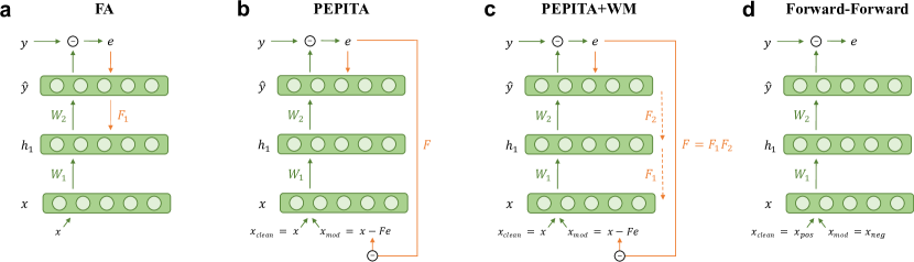
Figure 1: Overview of different error transportations and weight mirroring configurations. Green arrows indicate forward paths and orange arrows indicate error paths. (a) Feedback alignment (FA). (b) Present the Error to Perturb the Input To modulate Activity (PEPITA). (c) PEPITA with Weight Mirroring. (d) Forward-Forward (FF).

These reasons motivated the development of alternative solutions to credit assignment, relying on learning dynamics that are more biologically realistic than BP. Among these, several algorithms modified the feedback path carrying the information on the error (Lillicrap et al., 2016b; Nøkland, 2016; Akrout et al., 2019; Clark et al., 2021) or the target (Lee et al., 2015; Frenkel et al., 2021) to each node, while maintaining the alternation between a forward and a backward pass. More recently, “forward-only” algorithms were developed, which consist of a family of training schemes that replace the backward pass with a second forward pass. These approaches include the Forward-Forward algorithm (FF) (Hinton, 2022) and the Present the Error to Perturb the Input To modulate the Activity learning rule (PEPITA) (Dellaferrera & Kreiman, 2022). Both algorithms present a clean input sample in the first forward pass (positive phase for FF, standard pass for PEPITA). In FF, the second forward pass consists in presenting the network with a corrupted data sample obtained by merging different samples with masks (negative phase). In PEPITA, instead, in the second forward pass the input is modulated through information about the error of the first forward pass (modulated pass). For simplicity, from now on we will denote the first and second forward pass as clean and modulated pass, respectively, for both FF and PEPITA. These algorithms avoid the issues of weight transport, non-locality, freezing of activity, and, partially, the update locking problem (Lillicrap et al., 2020). Furthermore, as they do not require precise knowledge of the gradients, nor any non-local information, they are well-suited for implementation in neuromorphic hardware. Indeed, the forward path can be treated as a black box during learning and it is sufficient to measure forward activations to compute the weight update.

Despite the promising results, the “forward-only” algorithms are still in their infancy. Most importantly, neither Hinton (2022) nor Dellaferrera & Kreiman (2022) present an analytical argument explaining why the algorithms work effectively. In addition, they present some biologically unrealistic aspects. For instance, the FF requires the generation of corrupted data and their presentation in alternation with clean data, while PEPITA needs to retain information from the first forward pass until the second forward pass, therefore the algorithm is local in space but not local in time. Additionally, the algorithms present a performance gap when compared with other biologically inspired learning rules, such as feedback alignment (FA). Our work addresses all the mentioned limitations of the “forward-only” algorithms, focusing on PEPITA, and discusses similarities and differences between the FF and the PEPITA frameworks. Here, we make the following contributions:

• We demonstrate that PEPITA can be formulated as a sum of Hebbian and anti-Hebbian terms, making it local both in space and in time (Sec. 3.1 and 3.3);

• We analytically show the equivalence of the Hebbian version of PEPITA with the Forward-Forward algorithm (Hinton, 2022) with top-down feedback (Sec. 3.2);

• We show that PEPITA effectively implements “feedback-alignment” with an adaptive feedback matrix that depends on the upstream weights (Sec. 4.1);

• Focusing on PEPITA, we use the above result to analytically characterize the online learning dynamics of “forward-only” algorithms and explain the phenomenon of alignment of forward weights and top-down connections observed in original work (Sec. 4.2);

• We demonstrate that PEPITA can be applied to networks deeper than those tested by Dellaferrera & Kreiman (2022) (Sec. 5);

• We propose two strategies to extend the weight mirroring (WM) method to training schemes other than FA and show that PEPITA enhanced with WM achieves better alignment, accuracy, and convergence (Sec. 6).

The code to reproduce the experiments and the details on the simulation parameters are available at this link.

2 Background and relevant work

2.1 Feedback Alignment and Weight mirroring

Several training rules for artificial neural networks (ANNs) have been proposed to break the weight symmetry constraint required by BP (Lillicrap et al., 2016b; Nøkland, 2016; Liao et al., 2016; Nøkland & Eidnes, 2019; Frenkel et al., 2021; Hazan et al., 2018; Kohan et al., 2018; Clark et al., 2021; Meulemans et al., 2021; Halvagal & Zenke, 2022; Journé et al., 2022). The Feedback Alignment (FA) algorithm (Lillicrap et al., 2016b) replaces the transposed forward weights $W$ in the feedback path with random, fixed (non-learning) weight matrices $F$, thereby solving the weight transport problem (Fig. 1a) (Lillicrap et al., 2016b). The feedback signals driving learning in the forward weights push the forward matrices to become roughly proportional to the transposes of the fixed feedback matrices. While FA achieves a performance close to BP on simple tasks such as MNIST and CIFAR-10 with relatively shallow networks, it fails to scale to complex tasks and architectures (Bartunov et al., 2018; Xiao et al., 2018; Moskovitz et al., 2018).

In order to improve FA’s performance, Akrout et al. (2019) proposed the Weight-Mirror (WM) algorithm, an approach to adjust the feedback weights as well as the forward weights, to improve their agreement. The network’s training consists of two alternating phases. In engaged mode, the forward weights $W$ are trained using the standard FA. In mirror mode, the initially random feedback weights $F$ are trained to approximate the transpose of the $W$. To avoid weight transport, the $F$s are adjusted only based on their input and output vectors. Each layer $\ell$ is given as input a noisy signal $\xi$ with zero-mean and equal variance $\sigma_{\xi}^{2}$, and outputs a signal $r=W_{\ell}\xi$. The input and output information is used to update the $F_{\ell}$ matrix with the transposing rule $\Delta F_{\ell}=\eta_{F}\xi r^{\top}$, where $\mathbb{E}[\xi r^{\top}]=\sigma_{\xi}^{2}W_{\ell}^{\top}$. As a consequence, $F$ integrates a signal that is proportional to $W^{\top}$ on average. The resulting increase in the alignment between the two matrices allows the FA enhanced with WM to train neural networks with complex architectures (ResNet-18 and ResNet-50) on complex image recognition tasks (ImageNet).

2.2 Theoretical analyses

The theoretical study of online learning with one-hidden-layer neural networks has brought considerable insights to statistical learning theory (Saad & Solla, 1995a, b; Riegler & Biehl, 1995; Goldt et al., 2020; Refinetti et al., 2021b). We leverage these works to understand learning with biologically plausible algorithms. Through similar analysis, Refinetti et al. (2021a) analytically confirmed the previous results of Lillicrap et al. (2016a); Nøkland (2016); Frenkel et al. (2021) showing that the key to learning with direct feedback alignment (DFA) is the alignment between the network’s weights and the feedback matrices, which allows for the DFA gradient to be aligned to the BP gradient. The authors further show that the fixed nature of the feedback matrices induces a degeneracy-breaking effect where, out of many equally good solutions, a network trained with DFA converges to the one that maximizes the alignment between feedforward and feedback weights. This effect, however, imposes constraints on the structure of the feedback weights for learning, and possibly explains the difficulty of training convolutional neural networks with DFA.

Bordelon & Pehlevan (2022) derived self-consistent equations for the learning curves of DFA and FA in infinite-width networks via a path integral formulation of the training dynamics and investigated the impact of feedback alignment on the inductive bias.

2.3 The PEPITA learning rule

Here, we introduce notation and summarize the original learning rule proposed by Dellaferrera & Kreiman (2022).

Given a fully connected network with $L$ layers, an input signal $x$, and one-hot encoded labels $y$ (Fig. 1b), we first perform a clean forward pass through the network. The hidden unit and output unit activations are computed as:

$$\begin{split}h_{1}&=\sigma_{1}(W_{1}x),\\ h_{\ell}&=\sigma_{\ell}(W_{\ell}h_{\ell-1})\;\text{ for }2\leq\ell\leq L,\end{split}$$ (1)

where $\sigma_{l}$ is the non-linearity at the output of the $\ell^{th}$ layer and $W_{\ell}$ is the matrix of weights between layers $\ell-1$ and $\ell$. At the modulated pass, the activations are computed as:

$$\begin{split}h_{1}^{err}&=\sigma_{1}(W_{1}(x-Fe)),\\ h_{\ell}^{err}&=\sigma_{\ell}(W_{\ell}h_{\ell-1}^{err})\;\text{ for }2\leq\ell\leq L,\end{split}$$ (2)

where $e\equiv h_{L}-y$ denotes the network error and $F$ is the fixed random matrix used to project the error on the input. We denote the output of the network either as $h_{L}$ or $\hat{y}$. After the two forward passes, the weights are updated according to the PEPITA learning rules for the first, intermediate, and final layers, respectively:

$$\Delta W_{1} =(h_{1}-h_{1}^{err})(x-Fe)^{\top};$$ (3)

$$\Delta W_{\ell} =(h_{\ell}-h_{\ell}^{err})(h_{\ell-1}^{err})^{\top}\;\text{ for }2\leq\ell<L;$$ (4)

$$\Delta W_{L} =e(h_{L-1}^{err})^{\top}.$$ (5)

Note that, compared to the original paper, we changed the sign convention to read $-Fe$ rather than $+Fe$ in (2) and (3). Because the distribution of $F$ entries is symmetric around zero, this has no consequence on the results. This change will appear useful when describing the weight mirroring applied to PEPITA in Section 6. Finally, the updates are applied depending on the chosen optimizer. For example, using stochastic gradient descent with learning rate $\eta$:

$$W(t+1)=W(t)-\eta\Delta W.$$ (6)

The pseudocode is reproduced in Sup. Section A.

2.4 The Forward-Forward algorithm

Analogously to PEPITA, the FF algorithm removes the need for a backward pass and consists instead of two forward passes per sample (Fig. 1d). The clean pass and the modulated pass operate on real data and on appropriately distorted data, respectively. The distorted data is generated to exhibit very different long-range correlations but very similar short-range correlations. This forces FF to focus on the longer-range correlations in images that characterize shapes. In practice, the modulated samples are hybrid images obtained by adding together one digit image times a mask with large regions of ones and zeros and a different digit image times the reverse of the mask.

In the clean pass, the weights are updated to increase a “goodness” in every hidden layer, and in the modulated pass to decrease it. Hinton (2022) proposes to use the sum of the squared neural activities as goodness and specifies that the best results are achieved by minimizing this quantity for positive data and maximizing it on negative data.

3 On the relationship between FF and PEPITA

In this section, we demonstrate that PEPITA is equivalent to a FF framework with top-down connections. First, propose a minor change to the PEPITA update rule that exposes its Hebbian foundation. This version can also be applied in a time-local fashion. We then analytically demonstrate that the update rule proposed in the Forward-Forward (FF) algorithm (Hinton, 2022) is essentially equivalent to PEPITA’s when the negative samples are based on high-level feedback.

3.1 PEPITA’s formulation as Hebbian and anti-Hebbian phases

In their paper, Dellaferrera & Kreiman (2022) mention that the presynaptic term ($h^{err}_{\ell-1}$) in the learning rule of eqn. (4) can be replaced interchangeably with the same term, computed instead during the first forward pass ($h_{\ell-1}$). Taking this a step further, we separate the brackets in eqn. (4) and mix the two choices for the presynaptic term obtaining an approximately equivalent rule for hidden layer weights:

$$\begin{split}\Delta W_{\ell}&=h_{\ell}h_{\ell-1}^{err\top}-h_{\ell}^{err}h_{\ell-1}^{err\,\top}\\ &\simeq h_{\ell}h_{\ell-1}^{\top}-h_{\ell}^{err}h_{\ell-1}^{err\,\top}.\end{split}$$ (7)

The learning rule (7) now contains two Hebbian terms, each a product of the activity of the presynaptic and the postsynaptic node. We dub this approximation PEPITA-Hebbian. Fig. 3a shows that the approximation in eqns. (7) has negligible impact on the accuracy.

Figure 2: (a) Test accuracy as a function of training epochs for experiments with the MNIST dataset and a one-hidden-layer network with 1024 hidden units and ReLU activation. The blue dots represent the “vanilla” PEPITA algorithm (without momentum) while the purple crosses mark the AFA approximation (eqn. 11). (b) Generalization error as a function of the training time for the experiments with the PEPITA algorithm (blue dots) and its AFA approximation (purple crosses), and the theoretical curves derived in the Sup. Section E marked by full lines. Parameters: $D=500$, $lr=.05$, erf activation, two hidden units in both teacher and student. (c) Alignment angle between the teacher and student second-layer weights $\tilde{W}_{2}^{\top}W_{2}$ (dark green), between the student and a degenerate solution (light green), and between the adaptive feedback matrix and the student $W_{2}^{\top}FW_{1}$ (orange) as a function of training time. (d) We plot the unit vectors in the direction of the student $W_{2}$, the adaptive feedback $W_{1}F$ and the teacher $\tilde{W}_{2}$ as well as the degenerate solutions. The time shots are taken at different training times, marked by vertical dashed lines in panel (c).

3.2 Similarities between the weight updates of PEPITA and FF

In FF, in the clean pass, the weights are updated to increase a “goodness” in every hidden layer, and in the modulated pass to decrease it, where the goodness can be the sum of the squared neural activities (in our notation, $\|h_{\ell}\|^{2}$, for the clean and $\|h_{\ell}^{err}\|^{2}$ for the modulated pass). Hinton (2022) chooses a loss based on the logistic function $\sigma$ applied to the goodness, minus a threshold, $\theta$: $p=\sigma\left(\|h_{l}\|^{2}-\theta\right)$. This choice emphasizes the separation between positive and negative representations. For simplicity, we work directly on the goodness. This is equivalent to minimizing, at each layer $\ell$, a loss function defined as:

$$J_{\ell}=\|h_{\ell}\|^{2}-\|h_{\ell}^{err}\|^{2},$$ (8)

We then compute a weight update for FF as the derivative of the loss function (8) with respect to the weights:

$$\begin{split}\frac{1}{2}\frac{\partial J_{\ell}}{\partial W_{\ell}}&=\frac{1}{2}\left(\frac{\partial\|h_{\ell}\|^{2}}{\partial W_{\ell}}-\frac{\partial\|h_{\ell}^{err}\|^{2}}{\partial W_{\ell}}\right)\\ &=\frac{1}{2}\left(\frac{\partial\|\sigma(W_{\ell}h_{\ell-1})\|^{2}}{\partial W_{\ell}}-\frac{\partial\|\sigma(W_{\ell}h_{\ell-1}^{err})\|^{2}}{\partial W_{\ell}}\right)\end{split}$$

$$\begin{split}&=\sigma(W_{\ell}h_{\ell-1})\odot\sigma^{\prime}(W_{\ell}h_{\ell-1})h_{\ell-1}^{\top}\\ &\quad-\sigma(W_{\ell}h_{\ell-1}^{err})\odot\sigma^{\prime}(W_{\ell}h_{\ell-1}^{err})h_{\ell-1}^{err\top}\\ &=(\sigma^{\prime}(W_{\ell}h_{\ell-1})\odot h_{\ell}h_{\ell-1}^{\top}\\ &\quad-\sigma^{\prime}(W_{\ell}h_{\ell-1}^{err})\odot h_{\ell}^{err}h_{\ell-1}^{err})\\ &=(h_{\ell}^{\prime}\odot h_{\ell})h_{\ell-1}^{\top}-(h_{\ell}^{err^{\prime}}\odot h_{\ell}^{err})h_{\ell-1}^{err\,\top}.\end{split}$$ (9)

where $\odot$ indicates the Hadamard product.

We note that the terms $h^{\prime}_{\ell}\equiv\sigma^{\prime}(W_{\ell}h_{\ell-1})$ and $h_{\ell}^{err^{\prime}}\equiv\sigma^{\prime}(W_{\ell}h_{\ell-1}^{err})$ can be omitted in the common case where $\sigma$ is a ReLU function because they are 0 if and only if $h_{\ell}$ is already 0, and equal 1 otherwise. Likewise, they are always equal to 1 if $\sigma$ is linear. In these cases, therefore

$$\begin{split}\frac{1}{2}\frac{\partial J_{\ell}}{\partial W_{\ell}}=h_{\ell}h_{\ell-1}^{\top}-h_{\ell}^{err}h_{\ell-1}^{err\,\top},\end{split}$$ (10)

which is equivalent to eqn. (7), apart from a factor $1/2$ that can be incorporated in the learning rate. Since both Hinton (2022) and Dellaferrera & Kreiman (2022) generally use ReLUs as activations functions, we conclude that the FF update rule with loss (8) is equivalent to the previously proposed PEPITA in terms of the weight update rule.

For other choices of activation functions $\sigma$, since the error term $Fe$ is much smaller than the input $x$, the derivative of the activations in the two forward passes are close enough to approximate $\sigma^{\prime}(W_{\ell}h_{\ell-1})\simeq\sigma^{\prime}(W_{\ell}h_{\ell-1}^{err})$. In this case, the equivalence between the two learning rules (7) and (8) is only approximate.

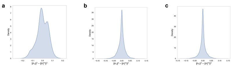
Figure 5: Difference of the norm of the squared activities of the first hidden layer between the clean and modulated pass in PEPITA (a) before training, (b) after 50 epochs, and (c) at the end of training. The network is a 2-hidden-layer network trained with WD with $\lambda=10^{-4}$ on the CIFAR-10 dataset. The activites are recorded on the test set. We remark that in PEPITA the input of the second forward pass is modulated by the error. Since the error decreases during training, also the difference of the activations in the two passes decreases with training. This explains why the distribution of the difference of the norm of the squared activities has a lower standard deviation in the middle of training (b) and at the end of training (c), than before training (a). In contrast, the modulation of the input in FF is constant during training, and the scope of training is maximising the difference of the goodness in the two passes.

We remark that the equivalence of PEPITA and FF holds for the general FF framework minimizing and maximizing the square of the activities. However, the weight update reported by Hinton (2022) presents analytical differences from (10) due to their use of thresholding and non-linearity applied to the goodness. Another notable difference lies in the way the “modulated” samples are generated in the two frameworks: as described, in PEPITA’s modulated pass, the input is modulated by the error. In the FF algorithm, in contrast, the negative samples are data vectors corrupted by external means, e.g. hybrid images in which one digit image times a binary mask and a different digit image times the reverse of the mask are added together. Furthermore, FF maximizes and minimizes the square of the activities for the clean pass and the modulated pass, respectively. In contrast, the activations of the two passes are not statistically different in PEPITA, presumably due to the small perturbation of the input in the second pass (Sup. Fig. 5).

3.3 Time locality

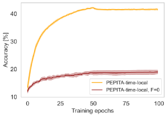
Figure 4: Test curve for PEPITA in its time-local formulation (Sec. 3.3) and time-local PEPITA with F=0 (i.e., only the last layer is trained) on the CIFAR-10 dataset. The network has 1 hidden layer with 1024 units. The forward matrices are initialized using the He normal initialization. $F$ entries are sampled from a normal distribution with standard deviation 0.5$\cdot 2\sqrt{6/(32\cdot 32\cdot 3)}$. We use learning rate $0.0001$ and weight decay with $\lambda=10^{-4}$. The learning is reduced by a factor of $\times 0.1$ at epoch 50. The solid line is the mean over 10 independent runs. The shaded colored area shows the standard deviation over the 10 runs. Time-local PEPITA achieves a significantly higher accuracy than the time-local, F=0 scheme.

Due to the negative sign in the gradient descent formulation, the first term of the PEPITA-Hebbian update (7) has an anti-Hebbian effect, while the second term is Hebbian. The weight update therefore consists of two separate phases that can contribute to learning without knowledge of the activity of the other, i.e. learning is time-local. Specifically, the term $h_{\ell}h_{\ell-1}^{\top}$ can be applied online, immediately as the activations of the first pass are computed. Analogously, the second term $-h_{\ell}^{err}h_{\ell-1}^{err\top}$ can be applied immediately during the second forward pass. Sup. Section A provides a pseudocode implementation of this version of the algorithm, which we name PEPITA-time-local. While PEPITA-Hebbian has the same accuracy as PEPITA (Fig. 3a), PEPITA-time-local has a negative impact on the network’s performance compared to the original formulation of PEPITA (Sup. Fig. 4). This decrease in accuracy may be related to the fact that in the original PEPITA, like in FA, DFA, and BP, the last layer is trained by delta-rule, while in the time-local version, the update of the last layer is split into two terms applied at different steps. To ensure that the hidden-layer updates prescribed by PEPITA are useful, we compared the test curve of PEPITA-time-local against a control with $F=0$ (Sup. Fig. 4), and found that removing the feedback decreases the accuracy from approx. 40% to approx. 18%. We leave the exploration to reduce the gap between PEPITA-time-local and PEPITA for further work.

Regarding the time-locality of FF, in FF the two forward passes can be computed in parallel, as the modulated pass does not need to wait for the computation of the error of the first pass. However, according to the available implementations (Mukherjee, 2023) the updates related to both passes are applied together at the end of the second forward pass.

Table 1: Test accuracy [%] achieved by BP, FA, DRTP, and PEPITA in the experiments, with and without weight decay, normalization of the activations and weight mirroring. Mean and standard deviation are computed over 10 independent runs. All training schemes are tested with ReLU nonlinearity except DRTP which uses tanh nonlinearity. The hyperparameters obtained through grid search are reported in Sup. Table 4. Bold fonts refer to the best results exclusively among PEPITA and its improvements.

	W. Decay	Norm.	Mirror	MNIST	CIFAR-10	CIFAR-100
BP	✗	✗	✗	98.72$\pm$0.06	57.60$\pm$0.20	29.36$\pm$0.19
	✓	✗	✗	98.66$\pm$0.04	57.92$\pm$0.19	29.93$\pm$0.27
FA	✗	✗	✗	98.48$\pm$0.05	56.76$\pm$0.23	22.75$\pm$ 0.28
	✓	✗	✗	98.35$\pm$0.04	57.19$\pm$0.24	22.62$\pm$0.25
DRTP	✗	✗	✗	95.45$\pm$0.09	46.92$\pm$0.21	16.99$\pm$0.16
	✓	✗	✗	95.44$\pm$0.09	46.92$\pm$0.27	17.59$\pm$0.18
PEPITA	✗	✗	✗	98.02$\pm$0.08	52.45$\pm$0.25	24.69$\pm$0.17
	✓	✗	✗	98.12$\pm$0.08	53.05$\pm$0.23	24.86$\pm$0.18
	✗	✓	✗	98.41$\pm$0.08	53.51$\pm$0.23	22.87$\pm$0.25
	✗	✗	✓	98.05$\pm$0.08	52.63$\pm$0.30	27.07$\pm$0.11
	✓	✗	✓	98.10$\pm$0.12	53.46$\pm$0.26	27.04$\pm$0.19
	✗	✓	✓	98.42$\pm$0.05	53.80$\pm$0.25	24.20$\pm$0.36

4 Theoretical analysis of the learning dynamics of PEPITA

In this section, we present a theory for the “forward-only” learning frameworks, focusing specifically on PEPITA in two-layer networks. We propose a useful approximation of the PEPITA update, that we exploit to derive analytic expressions for the learning curves, and investigate its learning mechanisms in a prototype teacher-student setup.

4.1 Taylor expansion and Adaptive Feedback rule

First, we observe that the perturbation applied in the modulation pass is small compared to the input: $\|Fe\|\ll\|x\|$. Indeed, in the experiments, the entries of the feedback matrix $F$ are drawn with standard deviation $\sigma_{F}=\kappa/\sqrt{D}$, where $D$ is the input dimension – typically large – and $\kappa$ is a constant set by grid search, while the input entries are of order one. Thus, it is reasonable to Taylor-expand the presynaptic term $h_{1}-h_{1}^{err}$, which results in the approximate update rule:

$$\Delta W_{1}\simeq\left[(W_{1}Fe)\odot h_{1}^{\prime}\right]x^{\top},$$ (11)

where we have used $x$ instead of $(x-Fe)$ since the small perturbation has been found to be negligible for the performance (Dellaferrera & Kreiman, 2022). Eqn. (11) shows that PEPITA is effectively implementing a “DFA-like” update (equivalent to FA in two-layer networks), but using an adaptive feedback (AF) matrix where the random term is modulated by the network weights. In light of this observation, it is natural to expect the alignment between $W_{1}F$ and $W_{2}$. This simple approximation, which we call Adaptive Feedback Alignment (AFA), is actually very accurate, as we verified numerically in Fig. 2a, displaying experiments on MNIST, and in Fig. 6 of Sup. Section D for the CIFAR-10 and CIFAR-100 datasets. AFA approximates PEPITA very accurately also in the teacher-student regression task depicted in Fig. 2b, which we study analytically in the next section.

4.2 ODEs for AFA with online learning for the teacher-student regression task

To proceed in our theoretical analysis, it is useful to assume a generative model for the data. We focus on the classical teacher-student setup (Gardner & Derrida, 1989; Seung et al., 1992; Watkin et al., 1993; Engel & Van den Broeck, 2001; Zdeborová & Krzakala, 2016). We consider $D-$dimensional standard Gaussian input vectors $x\sim\mathcal{N}(0,I_{D})$, while the corresponding label $y=\tilde{W}_{2}\,\tilde{\sigma}(\tilde{W}_{1}x)$ is generated by a two-layer teacher network with fixed random weights $\tilde{W}_{1}$, $\tilde{W}_{2}$ and activation function $\tilde{\sigma}(\cdot)$. The two-layer student network outputs a prediction $\hat{y}=W_{2}\,\sigma(W_{1}x)$ and is trained with the AFA rule and an online (or one-pass) protocol, i.e., employing a previously unseen example $x_{\mu}$, $\mu=1,\ldots,N$, at each training step. We characterize the dynamics of the mean-squared generalization error

$$\epsilon_{g}\equiv\frac{1}{2}\mathbb{E}_{x}{\left[(\hat{y}-y)^{2}\right]}\equiv\frac{1}{2}\mathbb{E}_{x}\left[{e^{2}}\right],\quad e\equiv\hat{y}-y,$$ (12)

in the infinite-dimensional limit of both input dimension and number of samples $D,N\rightarrow\infty$, at a rate $N/D\sim\mathcal{O}(1)$ where the training time is $t=\mu/D$. The hidden-layer size is of order one in both teacher and student. We follow the derivation in the seminal works of Biehl & Schwarze (1995); Saad & Solla (1995d, c), which has been put on rigorous ground by Goldt et al. (2019), and extend it to include the time-evolution of the adaptive feedback. As discussed in detail in Sup. Section E, the dynamics of the error $\epsilon_{g}$ as a function of training time $t$ is fully captured by the evolution of the AF matrix and a set of low-dimensional matrices encoding the alignment between student and teacher. We derive a closed set of ODEs tracking these key matrices, and we integrate them to obtain our theoretical predictions. Furthermore, in Sup. Section E.1, we perform an expansion at early training times $t\ll 1$, which elucidates the alignment mechanism and the importance of the “teacher-feedback alignment”, i.e. $\tilde{W}_{2}\tilde{W}_{1}F$, as well as the norm of $\|\tilde{W}_{1}F\|$.

For the sake of the discussion, we consider sigmoidal activations $\tilde{\sigma}(\cdot)=\sigma(\cdot)={\rm erf}(\cdot)$, keeping in mind that the symmetry ${\rm erf}(-x)=-{\rm erf}(x)$ induces a degeneracy of solutions.

Fig. 2b shows our theoretical prediction for the generalization error as a function of time, compared to numerical simulations of the PEPITA and AFA algorithms. We find excellent agreement between our infinite-dimensional theory and experiments, even at moderate system size $(D=500)$.

Fig. 2c shows the dynamic changes in the alignment of the second-layer student weights $W_{2}$ with different matrices: the AF matrix $W_{1}F$, the second-layer teacher weights $\tilde{W}_{2}$, the second-layer teacher weights of the closest degenerate solution. We clearly observe that the error is stuck at a plateau until “adaptive-feedback alignment” happens ($t\sim 10^{3}$). The lower panel depicts the directions of $W_{2}$, $W_{1}F$, and $\tilde{W}_{2}$ at different times, marked by vertical dashed lines in the above panel. It is crucial to notice that, in this case, the feedback matrix also evolves in time, giving rise to a richer picture, that we further discuss in Sup. Section D. In the special case of Fig. 2c, while the direction of $W_{1}F$ is almost constant, its norm increases, speeding up the learning process, as shown in Fig. 7. Similar behavior was observed in Dellaferrera & Kreiman (2022).

5 Testing PEPITA on deeper networks

The theoretical analysis above focuses on a two-layer network, as used in the proof-of-principle demonstration of PEPITA’s function in the original article. To the best of our knowledge, PEPITA has been tested so far only on two-layer networks. Since we consider this its most severe limitation until now, here, we use simulations to show that the algorithm can be extended to train deeper networks.

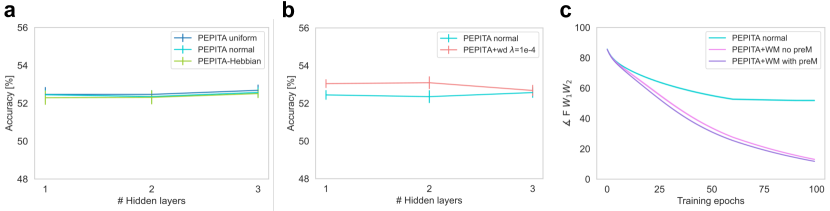
Figure 3: (a), (b) Test accuracy of fully connected networks with increasing depth trained with PEPITA on the CIFAR-10 dataset. (a) PEPITA uniform and PEPITA normal refer to the initialization of the weights and $F$ (Sec. 5.1). “PEPITA-Hebbian” refers to the learning rule explained in Section  3.1. (b) Effect of weight decay. (c) Alignment angle between $F$ and $W_{tot}$ during training with or without WM. PreM refers to pre-mirroring (Sec. 6.1). The hyperparameters are reported in Sup. Table 4.

5.1 Methods

We applied PEPITA to train fully connected models with up to five hidden layers. We tested two initialization strategies, He uniform (as in Dellaferrera & Kreiman, 2022) and He normal. F is initialized by sampling its entries from a uniform or normal distribution, respectively. This distribution has a mean of zero and standard deviation reported in Sup. Tab. 4. When not specified, we used the He normal initialization. Furthermore, we enhanced the basic operations of PEPITA with standard techniques in machine learning, namely weight decay (WD) (Krogh & Hertz, 1991) and activation normalization (as in Hinton, 2022). For all simulations, we tuned the hyperparameters by grid search. The optimal parameters are reported in Sup. Table 4.

5.2 Results

Regarding the initialization schemes, we verified that He uniform and normal performed equally (Fig. 3a). Weight decay and activation normalization improved the network’s accuracy (Fig. 3b and Table 1). On a one-hidden-layer network trained on the CIFAR-10 dataset, weight decay and normalization improved PEPITA’s performance by 0.6% and 1.1%, respectively (Fig. 3b and Table 1).

We compared PEPITA’s performance to three baselines, BP, FA, and Direct Random Target Projection (DRTP, Frenkel et al., 2021) with and without weight decay. For the baselines, we used the code by Frenkel et al. (2021). Our use of learning rate decay meant the grid search returned different hyperparameters, which explains some discrepancies in the accuracies compared to Frenkel et al. (2021).

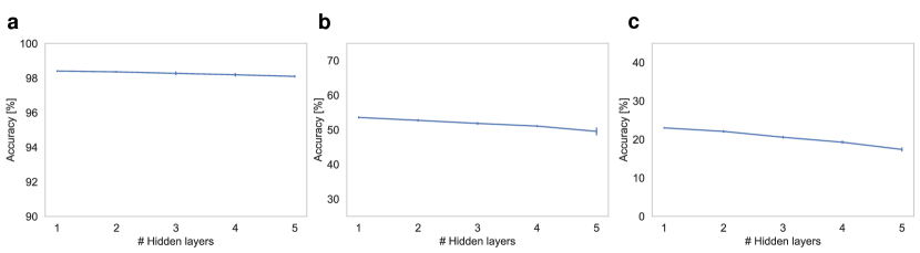
Figure 8: Test accuracy obtained with PEPITA and normalization of the activations for 1- to 5-hidden-layer networks on (a) MNIST, (b) CIFAR-10, and (c) CIFAR-100. Note that compared to Fig. 3 the trend is decreasing, as here we used activation normalization to obtain convergence for 4 and 5 hidden layers, which we did not use for Fig. 3.

Overall, we observe that PEPITA is able to train networks with three hidden layers without loosing accuracy with depth (Fig. 3a). Furthermore, with normalization of the activations, networks with up to five hidden layers can be trained, however they exhibit a decrease in performance (Sup. Fig. 8).

6 Enhancing PEPITA with weight mirroring

Besides adding more layers, we can also work on improving the performance of PEPITA and narrowing the gap with BP. In Section 4.1, we have shown that PEPITA is closely related to FA. Therefore, it is natural to adopt the weight mirror (WM) algorithm (Akrout et al., 2019), which has been shown to greatly improve alignment between the forward and backward connections and the consequent accuracy of FA. Here, we propose a generalization of WM for learning rules where the dimensionalities of the feedback and feedforward weights do not match, such as PEPITA, but also including DFA.

6.1 Methods

In a network trained with FA, the WM algorithm aligns, for each layer $\ell$, a backward matrix $F_{\ell}$ with the transpose of the corresponding forward matrix $W_{\ell}$ (Fig. 1a). In PEPITA, there is no one-to-one correspondence between forward and backward connections, as there is only one projection matrix $F$ (Fig. 1b). In order to recover the one-to-one correspondence of WM, we propose to factorize the $F$ matrix into the product of as many matrices as the number of layers: $F=\prod_{\ell=1}^{L}F_{\ell}$ (Fig. 1c). We initialize each of these matrices by sampling the entries from a normal distribution, then apply WM layer-wise. Note that this strategy could be applied to enhance other training schemes, such as DFA, with WM.

After each standard WM update, we also normalize each $F_{\ell}$ multiplying it by a factor $\left(\sigma_{F}^{(0)}/\sigma_{F}^{(t)}\right)^{1/L}$. This keeps the standard deviation $\sigma_{F}^{(t)}$ of the updated $F$ at step $t$ constant at its initialization value ($\sigma_{F}^{(0)}$, see Sup. Table 4). This is because PEPITA is sensitive to the magnitude of the feedback $\|Fe\|$, which must be kept non-zero for learning, but small enough for the approximation (11) to be valid. WM can be applied even before learning starts, to bring the initial random weights into alignment. This configuration is called pre-mirroring. We benchmarked our networks both with five epochs of pre-mirroring, and without.

6.2 Results

Alignment

Fig. 3c shows that, when weight mirroring is applied, the $W$ and $F$ matrices achieve a better alignment than with the standard PEPITA. The improvement of the alignment is more enhanced for one- and two-hidden-layer than for three-hidden-layer networks (Sup. Fig. 10).

Accuracy

The improved alignment obtained with WM is reflected in improved accuracy, especially for one-hidden-layer networks (Table 1), but also for two- and three-hidden-layer networks (Sup. Table 2). Remarkably, on the CIFAR-10 dataset, WM combined with activation normalization leads to 53.8%, an improvement of 1.3% compared to the standard PEPITA. On CIFAR-100 WM improves the accuracy by over 2%, reducing the gap with BP.

Convergence rate

The original paper reported that PEPITA’s convergence rate is in between BP (the fastest) and FA (the slowest). Here, we demonstrate that we can narrow the gap with BP by using pre-mirroring. We evaluate the learning speed using the plateau equation for learning curves proposed in Dellaferrera et al. (2022). By fitting the test curve to this function, we extract the slowness parameter, which quantifies how fast the network reduces the error during training.

With pre-mirroring, the convergence rate improves for one-hidden-layer models, as quantified by the lower slowness (Sup. Table 3). This is compatible with the “align, then memorize” paradigm (Refinetti et al., 2021a): pre-mirroring already provides the initial alignment phase as part of weight initialization, before the network sees the data.

7 Discussion

In the quest for biologically inspired learning mechanisms, the FF algorithm (Hinton, 2022) and the PEPITA algorithm (Dellaferrera & Kreiman, 2022) are “forward-only” algorithms which train neural networks with local information, without weight transport, without freezing the network’s activity, and without backward locking. Here, we first demonstrate that PEPITA is a special case of the FF framework, where the input to the second forward pass is provided by top-down feedback connections. The main difference between the two algorithms is in how the negative samples are generated. In FF, they are built by overlapping two different images according to binary masks. In PEPITA, they are built by integrating error information $e$ to the clean image. Thus, the error-driven generation of the input samples avoids the biologically unrealistic requirement of corrupting the images entailed by FF. Hinton (2022) himself suggests the alternative possibility that the negative data may be predicted by the neural net using top-down connections, rather than being externally provided. PEPITA is precisely an example of this possibility, which is compatible with biological mechanisms of neuromodulation and thalamo-cortical projections.

Through approximations of the PEPITA learning rule, we demonstrate that the updates can be written in a version which is local both in time and in space. Both time locality and the Hebbian formulation are relevant to the biological plausibility of PEPITA: to learn, each synapse needs no information about the past activity, or about the state of other synapses. This is believed to be the case for biological networks (Sjöström et al., 2001; Caporale & Dan, 2008; Markram et al., 2011), so that much contemporary literature in computational neuroscience is dedicated to finding local, bio-plausible learning algorithms (Richards et al., 2019; Lillicrap et al., 2020). Locality in time, moreover, would be especially important in the perspective of an implementation on an analog neuromorphic chip, where storing data in memory is difficult and online learning is desirable (Mitra et al., 2008; Demirag et al., 2021; Khacef et al., 2022).

Focusing on PEPITA, we show that its update rule can be approximated by an FA-like algorithm, where the error is propagated to the input layer via the project matrix $F$ “adapted” through the forward synaptic matrix. We perform a theoretical characterization of the generalization dynamics that provides intuition on the alignment mechanisms. This offers novel theoretical insight into the family of forward-only learning algorithms and links together PEPITA, Forward-Forward, and Feedback Alignment. In the future, we envision that further research could build a unified theoretical framework for these and other forward-only algorithms, leading to higher accuracy, network depth, and biological plausibility.

Appendix A Pseudocode for PEPITA

Algorithm 1 describes the original PEPITA as presented in Dellaferrera & Kreiman (2022).
Algorithm 2 describes our modification of PEPITA, which is Hebbian and local both in space and in time (Pepita-time-local). Algorithm 1 Implementation of PEPITA 0:  Input $x$ and one-hot encoded label $y$   # standard forward pass   $h_{0}=x$   for $\ell=1,...,L$ do      $h_{\ell}=\sigma_{\ell}(W_{\ell}h_{\ell-1})$   end for   $e=h_{L}-y$   # modulated forward pass   $h_{0}^{err}=x+Fe$   for $\ell=1,...,L$ do      $h_{\ell}^{err}=\sigma_{\ell}(W_{\ell}h_{\ell-1}^{err})$      if $\ell<L$ then         $\Delta W_{\ell}=(h_{\ell}-h_{\ell}^{err})(h_{\ell-1}^{err})^{\top}$      else         $\Delta W_{\ell}=e(h_{\ell-1}^{err})^{\top}$      end if      $W_{\ell}(t+1)=W_{\ell}(t)-\eta\Delta W_{\ell}$ # apply update   end for Algorithm 2 Implementation of PEPITA-time-local 0:  Input $x$ and one-hot encoded label $y$   # standard forward pass   $h_{0}=x$   for $\ell=1,...,L$ do      $h_{\ell}=\sigma_{\ell}(W_{\ell}h_{\ell-1})$      $\Delta W_{\ell}^{+}=h_{\ell}h_{\ell-1}^{\top}$      $W_{\ell}^{+}(t+1)=W_{\ell}(t)-\eta\Delta W_{\ell}^{+}$ # apply 1st update   end for   $e=h_{L}-y$   # modulated forward pass   $h_{0}^{err}=x-Fe$   for $\ell=1,...,L$ do      $h_{\ell}^{err}=\sigma_{\ell}(W_{\ell}^{+}h_{\ell-1}^{err})$      if $\ell<L$ then         $\Delta W_{\ell}^{-}=-h_{\ell}^{err}h_{\ell-1}^{err\top}$      else         $\Delta W_{\ell}^{-}=-yh_{\ell-1}^{err\top}$      end if      $W_{\ell}(t+1)=W_{\ell}^{+}(t+1)-\eta\Delta W_{\ell}^{-}$ # apply 2nd update   end for

The updates for PEPITA-Hebbian are:

• for the hidden layers:

$$\begin{split}\Delta W_{\ell}&=h_{\ell}h_{\ell-1}^{err\top}-h_{\ell}^{err}h_{\ell-1}^{err\,\top}\\ &\simeq h_{\ell}h_{\ell-1}^{\top}-h_{\ell}^{err}h_{\ell-1}^{err\,\top},\end{split}$$ (13)

• for the first and last layers

$$\begin{split}\Delta W_{1}&\simeq h_{1}x^{\top}-h_{1}^{err}(x-Fe)^{\top};\\ \Delta W_{L}&\simeq h_{L}h_{L-1}^{\top}-yh_{L-1}^{err\,\top}.\end{split}$$ (14)

These updates are applied at the end of both forward passes for PEPITA-Hebbian, similarly as in pseudocode 1.

Appendix B Training with the time-local rule

Appendix C Distribution of the goodness in PEPITA

Appendix D Additional figures on the AFA approximation

Fig. 6 displays the comparison between the “vanilla” PEPITA algorithm and the AFA approximation introduced in eqn. (11) of the main text. The test accuracy as a function of training epochs is depicted for the CIFAR-10 dataset in the left panel and for the CIFAR-100 dataset in the right panel.

Fig. 7 depicts the norm of the adaptive feedback matrix $f=W_{1}F/D$ as a function of training time. The symbols mark the numerical simulations at dimension $D=500$, while the full line represents our theoretical prediction. We observe that, for this run, the norm of the adaptive feedback increases over time. We have observed by numerical inspection that this behavior is crucial to speed up the dynamics, as also observed in (Dellaferrera & Kreiman, 2022).

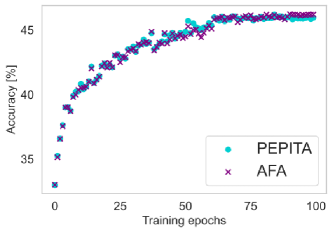
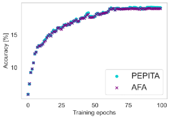
Figure 6: Comparison between the test accuracy as a function of training epochs between the “vanilla” PEPITA algorithm and its AFA approximation (eqn. (11) of the main text) for the CIFAR-10 (left panel) and CIFAR-100 (right panel) datasets.

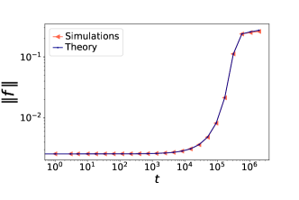
Figure 7: Norm of the alignment matrix $f=W_{1}F/D$ as a function of training time, for the same parameters as in Fig. 2 of the main text: $D=500$, $lr=.05$, erf activation, two hidden units in both teacher and student ($K=M=2$).

Appendix E ODEs for online learning in the teacher-student regression task

In this section, we present the details of the teacher-student model under consideration and we sketch the derivation of the ordinary differential equations (ODEs) tracking the online learning dynamics of the AFA rule. We consider a shallow student network trained with AFA to solve a supervised learning task. The input data are random $D-$dimensional vectors $x\in\mathbb{R}^{D}$ with independent identically distributed (i.i.d.) standard Gaussian entries $x_{j}\sim\mathcal{N}(0,1)$, $j=1,\ldots,D$, and the (scalar) labels are generated as the output of a one-hidden-layer teacher network with parameters $\tilde{\theta}=(\tilde{W}_{1},\tilde{W}_{2},M,\tilde{\sigma})$:

$$y =\sum_{m=1}^{M}\tilde{W}_{2}^{m}\tilde{\sigma}(\nu^{m}),\qquad\nu^{m}=\frac{\tilde{W}_{1}^{m}\,x}{\sqrt{D}},$$ (15)

where $M$ is the size of the teacher hidden layer, $\nu^{m}$ denotes the teacher preactivation at unit $m\in\{1,\ldots,M\}$, and $\tilde{\sigma}(\cdot)$ is the activation function. The student is a one-hidden-layer neural network parametrized by $\theta=(W_{1},W_{2},K,\sigma)$ that outputs the prediction

$$\hat{y}=\sum_{k=1}^{K}W_{2}^{k}\sigma(\lambda^{k}),\qquad\lambda^{k}=\frac{W_{1}^{k}x}{\sqrt{D}},$$ (16)

where $K$ is the size of the student hidden layer, $\sigma(\cdot)$ the student activation function, $\lambda^{k}$ the student preactivation at unit $k\in\{1,\ldots,K\}$. For future convenience, we write explicitly the scaling with respect to the input dimension. Therefore, at variance with the main text, in this supplemementary section we always rescale the first layer weights as well as the feedback by $1/\sqrt{D}$.

We focus on the online (or one-pass) learning protocol, so that at each training time the student network is presented with a fresh example $x_{\mu}$, $\mu=1,\ldots N$, and $N/D\sim\mathcal{O}(1)$. The weights are updated according to the Adaptive Feedback Alignment (AFA) rule defined in eqn. (11):

$$W_{1}(\mu+1)=W_{1}(\mu)-\eta_{1}\Delta W_{1}(\mu), \Delta W_{1}=\frac{W_{1}F}{D}e\,h^{\prime}_{1}\frac{x^{\top}}{\sqrt{D}},$$ (17)

$$W_{2}(\mu+1)=W_{2}(\mu)-\eta_{2}\Delta W_{2}(\mu), \Delta W_{2}=e\,h_{1}^{\top}.$$ (18)

We consider fixed learning rates $\eta_{1}=\eta$, $\eta_{2}=\eta/D$. Different learning rate regimes have been explored in (Veiga et al., 2022). It is crucial to notice that the mean squared generalization error

$$\epsilon_{g}(\theta,\tilde{\theta}) =\frac{1}{2}\mathbb{E}_{x}\left[\left(\sum_{k=1}^{K}W_{2}^{k}\sigma(\lambda^{k})-\sum_{m=1}^{M}\tilde{W}_{2}^{m}\tilde{\sigma}(\nu^{m})\right)^{2}\right]$$ (19)

depends on the high-dimensional input expectation only through the low-dimensional expectation over the preactivations $\{\lambda_{k}\}_{k=1}^{K},\{\nu_{m}\}_{m=1}^{M}$. Notice that, in this online-learning setup, the input $x$ is independent of the weights, which are held fixed when taking the expectation. Furthermore, due to the Gaussianity of the inputs, the preactivations are also jointly Gaussian with zero mean and second moments:

$$Q^{kl}=\mathbb{E}_{x}\left[\lambda^{k}\lambda^{l}\right]=\frac{W_{1}^{k}\cdot W_{1}^{l}}{D}\;, R^{km}=\mathbb{E}_{x}\left[\lambda^{k}\nu^{m}\right]=\frac{W_{1}^{k}\cdot{\tilde{W}_{1}}^{m}}{D}\;, T^{mn}=\mathbb{E}_{x}\left[\nu^{m}\nu^{n}\right]=\frac{{\tilde{W}_{1}}^{m}\cdot{\tilde{W}_{1}}^{n}}{D}.$$ (20)

The above matrices are named order parameters in the statistical physics literature and play an important role in the interpretation. The matrices $Q$ and $T$ capture the self-overlap of the student and teacher networks respectively, while the matrix $R$ encodes the teacher-student overlap. In the infinite-dimensional limit discussed above, the generalization error is only a function of the order parameters $Q,T,R$ and of the second layer weights $\tilde{W}_{2},W_{2}$ of teacher and student respectively. Therefore, by tracking the evolution of these matrices via a set of ODEs – their “equations of motion” – we obtain theoretical predictions for the learning curves. The update equations for $Q,R,W_{2}$ can be obtained from eqns. (17) according to the following rationale. As an example, we consider the update equation for the matrix $Q$:

$$\begin{split}Q^{kl}(\mu+1)-Q^{kl}(\mu)&=\frac{1}{D}\left[W_{1}^{k}(\mu)-\eta\Delta W_{1}^{k}(\mu)\right]\cdot\left[W_{1}^{l}(\mu)-\eta\Delta W_{1}^{l}(\mu)\right]-\frac{1}{D}W_{1}^{k}(\mu)\cdot W_{1}^{l}(\mu)\\ &=-\frac{1}{D}\eta\,f^{k}\,e\,\sigma^{\prime}(\lambda^{k})\lambda^{l}-\frac{1}{D}\eta\,f^{l}\,e\,\sigma^{\prime}(\lambda^{l})\lambda^{k}+\frac{1}{D}\eta^{2}\,f^{k}\,f^{l}\,\sigma^{\prime}(\lambda^{k})\sigma^{\prime}(\lambda^{l})e^{2},\end{split}$$ (21)

where we have defined the adaptive feedback $f:=W_{1}F/D$, we have used that $\|x_{\mu}\|^{2}=D$ as $D\rightarrow\infty$ and omitted the $\mu-$dependence on the right hand side for simplicity. By taking $t=\mu/D$, as shown in (Goldt et al., 2019), in the infinite-dimensional limit $Q^{kl}(\mu)$ concentrates to the solution of the following ODE:

$$\frac{{\rm d}Q^{kl}}{{\rm d}t} =-\eta f^{k}\mathbb{E}\left[\sigma^{\prime}(\lambda^{k})\lambda^{l}e\right]-\eta f^{l}\mathbb{E}\left[\sigma^{\prime}(\lambda^{l})\lambda^{k}e\right]+\eta^{2}f^{k}f^{l}\mathbb{E}\left[\sigma^{\prime}(\lambda^{k})\sigma^{\prime}(\lambda^{l})e^{2}\right],$$ (22)

Similarly, we can derive ODEs for the evolution of $R,W_{2}$ and the adaptive feedback $f$:

$$\frac{{\rm d}R^{km}}{{\rm d}t}=-\eta\,f^{k}\mathbb{E}\left[\sigma^{\prime}(\lambda^{k})\nu^{m}e\right], \frac{{\rm d}W_{2}^{k}}{{\rm d}t}=-\eta\mathbb{E}\left[\sigma(\lambda^{k})e\right], \frac{{\rm d}f^{k}}{{\rm d}t}=-\eta f^{k}\mathbb{E}\left[\rho\sigma^{\prime}(\lambda^{k})e\right],$$ (23)

where the expectations are taken over the preactivatons and $\rho={F\,x}/{\sqrt{D}}$, and we have $\mathbb{E}_{x}[\lambda^{k}\rho]=f^{k}$, $\mathbb{E}_{x}[\nu^{m}\rho]=\tilde{f}^{m}:=\tilde{W}_{1}F/D$, $q_{f}:=F\cdot F/D$. The generalization error can be rewritten as

$$\lim_{D\rightarrow\infty}\epsilon_{g}(\theta,\tilde{\theta})=\frac{1}{2}\sum_{k,l=1}^{K}W_{2}^{k}W_{2}^{l}\,I_{2}(k,l)+\frac{1}{2}\sum_{m,n=1}^{M}\tilde{W}_{2}^{m}\tilde{W}_{2}^{n}\,I_{2}(m,n)-\sum_{k=1}^{K}\sum_{m=1}^{M}W_{2}^{k}\tilde{W}_{2}^{m}\,I_{2}(k,m),$$ (24)

where $I_{2}$ generically encodes the averages over the activations

$$I_{2}(\alpha,\beta)=\mathbb{E}\left[\sigma_{\alpha}(\gamma^{\alpha})\sigma_{\beta}(\gamma^{\beta})\right], \gamma^{\alpha}=\begin{cases}\lambda^{k}&\textrm{if}\;\;\alpha=k,l\\ \nu^{m}&\textrm{if}\;\;\alpha=m,n\end{cases}, \sigma_{\alpha}=\begin{cases}\sigma&\textrm{if}\;\;\alpha=k,l\\ \tilde{\sigma}&\textrm{if}\;\;\alpha=m,n\end{cases}.$$ (25)

The other averages in eqns. can be expressed in a similar way and estimated by Monte Carlo methods. In the case of sigmoidal activation $\sigma(x)={\rm erf}(x/\sqrt{2})$, the function $I_{2}$ has an analytic expression.

$$I_{2}(\alpha,\beta)=\frac{2}{\pi}{\rm arcsin}\frac{C^{\alpha\beta}}{\sqrt{1+C^{\alpha\alpha}}\sqrt{1+C^{\beta\beta}}}\;, C^{kl}=Q^{kl},\;\;C^{km}=R^{km},\;\;C^{mn}=T^{mn}.$$ (26)

E.1 Early-training expansion

As done by (Refinetti et al., 2021a) for DFA, it is instructive to consider an expansion of the ODEs at early training times. We assume the following initialization: $W_{2}^{k}(0)=0$, $\forall k\in\{1,\ldots,K\}$, while the first layer is assumed to be orthogonal to the teacher $W_{1}^{k}(0)\cdot\tilde{W}_{1}^{m}=0$ and of fixed norm $\|W_{1}^{k}(0)\|^{2}/D=q_{0}$, $\forall k\in\{1,\ldots,K\},\forall m\in\{1,\ldots,M\}$. We also take orthogonal first-layer teacher weights, such that $T$ is the identity matrix. This initialization leads to:

$$R^{km}(0)=0\;, \frac{{\rm d}}{{\rm d}t}W_{2}^{k}\biggr{\rvert}_{t=0}=0\;, \frac{{\rm d}}{{\rm d}t}R^{km}\biggr{\rvert}_{t=0}=\frac{\sqrt{2}}{\pi\sqrt{1+q_{0}}}\eta\,f^{k}(0)\,\tilde{W}_{2}^{m}.$$ (27)

We can therefore compute the second-layer update to linear order:

$$\frac{{\rm d}}{{\rm d}t}W_{2}^{k}(t)=\frac{2}{\pi^{2}(1+q_{0})}\eta^{2}\,f^{k}(0)\,\|\tilde{W}_{2}\|_{2}^{2}\;t+\mathcal{O}(t^{2}).$$ (28)

Eqn. (28) shows that the update of the second-layer weights at early training times is in the direction of the adaptive feedback matrix, in agreement with the alignment phase observed in experiments. Crucially, it is necessary that $f^{k}(0)\neq 0\;\forall k$ in order to have non-zero updates, i.e. the feedback $F$ must not be orthogonal to the first-layer weights at initialization. We now inspect the behavior of the adaptive feedback at the beginning of training. We have that the update at time zero is:

$$\frac{{\rm d}}{{\rm d}t}f^{k}\biggr{\rvert}_{t=0}=\frac{2}{\pi}\,\eta\frac{f^{k}(0)}{\sqrt{(1+q_{0})(1+q_{f})-f^{k}(0)^{2}}}\,(\tilde{W}_{2}\cdot\tilde{f}),$$ (29)

and

$$f^{k}(t)=f^{k}(0)+\frac{2}{\pi}\,\eta\frac{f^{k}(0)}{\sqrt{(1+q_{0})(1+q_{f})-f^{k}(0)^{2}}}\,(\tilde{W}_{2}\cdot\tilde{f})\;t+\mathcal{O}(t^{2}).$$ (30)

Eqn. (29) illustrates that the feedback-teacher alignment $\tilde{f}$ plays an important role in speeding up the dynamics. Indeed, if $\|\tilde{f}\|_{2}^{2}$ is close to zero, the feedback update slows down inducing long plateaus in the generalization error. A similar role is played by the alignment angle between $\tilde{W}_{2}$ and $\tilde{f}$.

Appendix F PEPITA’s results compared to the Baselines

Table 2: Test accuracy [%] achieved by BP, FA, DRTP, PEPITA, and PEPITA with weight mirroring in the experiments. Mean and standard deviation are computed over 10 independent runs. The nonlinearity is ReLU for all algorithms except DRTP, for which is tanh. WM was used in combination with weight decay with $\lambda=10^{-4}$ for the networks trained on the CIFAR-10 dataset and for the 3-hidden-layer networks trained on the CIFAR-100 dataset. The other networks are trained without weight decay. Bold fonts refer to the best results exclusively among PEPITA and its improvements.

	2 hidden layers			3 hidden layers
	MNIST	CIFAR-10	CIFAR-100	MNIST	CIFAR-10	CIFAR-100
BP	98.85$\pm$0.06	59.69$\pm$0.25	32.28$\pm$0.17	98.89$\pm$0.04	60.07$\pm$0.28	32.80$\pm$0.16
FA	98.64$\pm$0.05	57.76$\pm$0.39	22.90$\pm$0.14	97.48$\pm$0.06	52.99$\pm$0.21	22.81$\pm$0.21
DRTP	95.36$\pm$0.09	47.48$\pm$0.19	20.55$\pm$0.30	95.74$\pm$0.10	47.44$\pm$0.19	21.81$\pm$0.24
PEPITA	98.19$\pm$0.07	52.39$\pm$0.27	24.88$\pm$0.15	95.07$\pm$0.11	52.47$\pm$0.24	01.00$\pm$0.00
PEPITA +WD	98.09$\pm$0.07	53.09$\pm$0.33	24.64$\pm$0.24	95.09$\pm$0.16	52.56$\pm$0.31	23.13$\pm$0.21
PEPITA +WM	98.13$\pm$0.05	53.44$\pm$0.28	26.95$\pm$0.24	96.33$\pm$0.12	52.80$\pm$0.33	23.03$\pm$0.28

Appendix G Slowness results

Table 3 shows that the best convergence rate for PEPITA (i.e., small slowness value) is obtained in general by PEPITA with Weight Mirroring (MNIST, CIFAR-100). Compared to the baselines, PEPITA has a better convergence than all the algorithms on MNIST, is the slowest on CIFAR-10, and the second best after BP on CIFAR-100. However, these results are strongly dependent on the chosen learning rate.

Table 3: Convergence rate in terms of slowness value obtained by BP, FA, DRTP and PEPITA in the experiments for the fully connected models trained on MNIST, CIFAR-10 and CIFAR-100 (same simulations reported in Table 1). PreM refers to pre-mirroring (Sec. 6.1). The smallest the slowness value, the better the convergence rate. The slowness is computed on the first 60 epochs of the test curve (before the learning rate decay), averaged over 10 independent runs. All the networks are trained without weight decay. The slowness result of FA on CIFAR-10 is lower than in (Dellaferrera & Kreiman, 2022) as our grid search returned a higher value for the learning rate. Bold fonts refer to the best results exclusively among PEPITA and its improvements.

	1$\times$1024 Fully connected models
	MNIST	CIFAR-10	CIFAR-100
BP	0.061$\pm$0.001	0.421$\pm$0.016	1.406$\pm$0.053
FA	0.081$\pm$0.002	0.463$\pm$0.020	4.946$\pm$0.123
DRTP	0.059$\pm$0.002	0.362$\pm$0.021	12.904$\pm$0.443
PEPITA	0.052$\pm$0.004	0.894$\pm$0.071	2.695$\pm$0.166
PEPITA+WM	0.047$\pm$0.005	0.890$\pm$0.081	2.333$\pm$0.102
PEPITA+WM+preM	0.040$\pm$0.002	0.856$\pm$0.051	1.999$\pm$0.059

Appendix H Hyperparameters

Table 4: 1-hidden-layer network architectures and settings used in the experiments. The nonlinearity is ReLU for all algorithms except DRTP, for which is tanh.

	1 Hidden layer			1 hidden layer - Normalization
	MNIST	CIFAR-10	CIFAR-100	MNIST	CIFAR-10	CIFAR-100
InputSize	28$\times$28$\times$1	32$\times$32$\times$3	32$\times$32$\times$3	28$\times$28$\times$1	32$\times$32$\times$3	32$\times$32$\times$3
Hidden units	1$\times$1024	1$\times$1024	1$\times$1024	1$\times$1024	1$\times$1024	1$\times$1024
Output units	10	10	100	10	10	100
$\eta$ BP	0.1	0.01	0.1	$-$	$-$	$-$
$\eta$ FA	0.1	0.01	0.01	$-$	$-$	$-$
$\eta$ DRTP	0.01	0.001	0.001	$-$	$-$	$-$
$\eta$ PEPITA	0.1	0.01	0.01	100	10	100
$\lambda$ weight decay	$10^{-5}$	$10^{-4}$	$10^{-5}$	0.0	0.0	0.0
$\eta$ decay rate	$\times$0.1	$\times$0.1	$\times$0.1	$\times$0.5	$\times$0.1	$\times$0.1
decay epoch	60,90	60,90	60,90	60,90	60,90	60,90
Batch size	64	64	64	64	64	64
$\eta$ WM	0.1	0.001	0.1	0.001	0.001	0.001
$\lambda$ weight decay WM	0.0	0.1	0.5	0.1	0.1	0.1
$\sigma_{F}^{(0)}$ (uniform)	0.05$\cdot 2\sqrt{\frac{6}{\text{fanin}}}$	0.05$\cdot 2\sqrt{\frac{6}{\text{fanin}}}$	0.05$\cdot 2\sqrt{\frac{6}{\text{fanin}}}$	0.05$\cdot 2\sqrt{\frac{6}{\text{fanin}}}$	0.05$\cdot 2\sqrt{\frac{6}{\text{fanin}}}$	0.05$\cdot 2\sqrt{\frac{6}{\text{fanin}}}$
$\sigma_{F}^{(0)}$ (normal)	0.05$\cdot\sqrt{\frac{2}{\text{fanin}}}$	0.05$\cdot\sqrt{\frac{2}{\text{fanin}}}$	0.05$\cdot\sqrt{\frac{2}{\text{fanin}}}$	0.05$\cdot\sqrt{\frac{2}{\text{fanin}}}$	0.05$\cdot\sqrt{\frac{2}{\text{fanin}}}$	0.05$\cdot\sqrt{\frac{2}{\text{fanin}}}$
Fan in	$28\cdot 28\cdot 1$	$32\cdot 32\cdot 3$	$32\cdot 32\cdot 3$	$28\cdot 28\cdot 1$	$32\cdot 32\cdot 3$	$32\cdot 32\cdot 3$
$\#$epochs	100	100	100	100	100	100
Dropout	10%	10%	10%	10%	10%	10%

Table 5: 2-, 3-hidden-layer network architectures and settings used in the experiments. The nonlinearity is ReLU for all algorithms except DRTP, for which is tanh. (*) For the 3-hidden-layer network trained with PEPITA on the MNIST dataset, we did not use learning rate decay, as indicated by the grid search.

	2 hidden layers			3 hidden layers
	MNIST	CIFAR-10	CIFAR-100	MNIST	CIFAR-10	CIFAR-100
InputSize	28$\times$28$\times$1	32$\times$32$\times$3	32$\times$32$\times$3	28$\times$28$\times$1	32$\times$32$\times$3	32$\times$32$\times$3
Hidden units	2$\times$1024	2$\times$1024	2$\times$1024	3$\times$1024	3$\times$1024	3$\times$1024
Output units	10	10	100	10	10	100
$\eta$ BP	0.1	0.01	0.1	0.1	0.01	0.1
$\eta$ FA	0.1	0.01	0.01	0.01	0.001	0.01
$\eta$ DRTP	0.001	0.001	0.001	0.001	0.001	0.001
$\eta$ PEPITA	0.1	0.01	0.01	0.001	0.01	0.01
$\lambda$ weight decay	$10^{-5}$	$10^{-4}$	$10^{-5}$	$10^{-5}$	$10^{-4}$	$10^{-4}$
$\eta$ decay rate (*)	$\times$0.1	$\times$0.1	$\times$0.1	$\times$0.1	$\times$0.1	$\times$0.1
decay epoch	60,90	60,90	60,90	60,90	60,90	60,90
Batch size	64	64	64	64	64	64
$\eta$ WM	0.00001	1.0	1.0	0.1	0.001	0.001
$\lambda$ WD WM	0.0	0.1	0.1	0.001	0.1	0.1
$\sigma_{F}^{(0)}$ (uniform)	0.05$\cdot 2\sqrt{\frac{6}{\text{fanin}}}$	0.05$\cdot 2\sqrt{\frac{6}{\text{fanin}}}$	0.05$\cdot 2\sqrt{\frac{6}{\text{fanin}}}$	0.05$\cdot 2\sqrt{\frac{6}{\text{fanin}}}$	0.05$\cdot 2\sqrt{\frac{6}{\text{fanin}}}$	0.05$\cdot 2\sqrt{\frac{6}{\text{fanin}}}$
$\sigma_{F}^{(0)}$ (normal)	0.05$\cdot\sqrt{\frac{2}{\text{fanin}}}$	0.05$\cdot\sqrt{\frac{2}{\text{fanin}}}$	0.05$\cdot\sqrt{\frac{2}{\text{fanin}}}$	0.05$\cdot\sqrt{\frac{2}{\text{fanin}}}$	0.05$\cdot\sqrt{\frac{2}{\text{fanin}}}$	0.05$\cdot\sqrt{\frac{2}{\text{fanin}}}$
Fan in	$28\cdot 28\cdot 1$	$32\cdot 32\cdot 3$	$32\cdot 32\cdot 3$	$28\cdot 28\cdot 1$	$32\cdot 32\cdot 3$	$32\cdot 32\cdot 3$
$\#$epochs	100	100	100	100	100	100
Dropout	10%	10%	10%	10%	10%	10%

Appendix I Training deeper fully-connected models

Appendix J Additional figures on weight mirroring

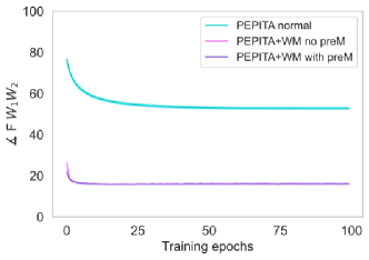
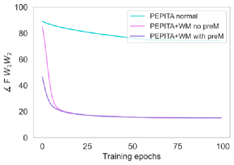
Figure 9: Alignment angle between $F$ and $W_{tot}$ during training with (pink and purple curves) or without (blue curve) WM for the MNIST (left panel) and CIFAR-100 (right panel) datasets. PreM refers to pre-mirroring (Sec. 6.1). The hyperparameters are reported in Sup. Table 4. The curves are averaged over 10 independent runs.

Figure 10: Alignment angle between $F$ and $W_{tot}$ during training with (pink curve) or without (blue curve) WM for the CIFAR-10 dataset for (a) 1-, (b) 2-, (c) 3-hidden-layer networks. The hyperparameters are reported in Sup. Table 4. The curves are averaged over 10 independent runs.

References

- Akrout et al. (2019) Akrout, M., Wilson, C., Humphreys, P., Lillicrap, T., and Tweed, D. Deep learning without weight transport. In NeurIPS, 2019.
- Bartunov et al. (2018) Bartunov, S., Santoro, A., Richards, B. A., Marris, L., Hinton, G. E., and Lillicrap, T. P. Assessing the scalability of biologically-motivated deep learning algorithms and architectures. In Proceedings of the 32nd International Conference on Neural Information Processing Systems, NIPS’18, pp. 9390–9400, 2018.
- Biehl & Schwarze (1995) Biehl, M. and Schwarze, H. Learning by on-line gradient descent. Journal of Physics A: Mathematical and general, 28(3):643, 1995.