Abstract
Our goal in this paper is to investigate the fluid picture associated with an open large scale storage network of non reliable file servers with finite capacity. In this storage system new files can be added and a file with only one copy can be lost or duplicated. The Skorokhod problem with oblique reflection in a bounded convex domain is used to identify the fluid limits. Such analysis involves the study of three different regimes, the under-loaded, the critical and the overloaded regime. The overloaded regime is of particular importance. To identify the fluid limits, new martingales are obtained and an averaging property is established. This paper is the continuation of the recent paper [4 ] .
Keywords :
Markov process, Skorokhod problem, Loss network,Exponential martingales, Ornstein-Uhlenbeck process,Hitting time.
1 Introduction
In this paper, we are concerned with an open large-scale storage system with non-reliable file servers in a communication network. The overall storage capacity is assumed to be limited.
In the network considered, servers can break down randomly and when the disk of a given server breaks down, its files are lost, but can be retrieved on the other servers if copies are available. In order to ensure persistence, a duplication mechanism of files to other servers is then performed. The goal is for each file to have at least one copy available on one of the servers as long as possible. Furthermore in order to use the bandwidth in an optimal way, there should not be too many copies of a given file so that the network can accommodate a large number of distinct files.
In the system considered here, if there is enough storage capacity, a file with one copy can be duplicated on the other servers aiming to guarantee persistence in the system and new files can be admitted to the system for storage, each with two copies, otherwise, if capacity doesn’t allow the new files are rejected and the duplication is blocked.
The natural critical parameters of the network are ( N , μ N , λ N , ξ N , F N ) 𝑁 subscript 𝜇 𝑁 subscript 𝜆 𝑁 subscript 𝜉 𝑁 subscript 𝐹 𝑁 (N,\mu_{N},\lambda_{N},\xi_{N},F_{N}) N 𝑁 N μ N subscript 𝜇 𝑁 \mu_{N} λ N subscript 𝜆 𝑁 \lambda_{N} ξ N subscript 𝜉 𝑁 \xi_{N} F N subscript 𝐹 𝑁 F_{N} F N subscript 𝐹 𝑁 F_{N} N 𝑁 N
lim N → + ∞ F N N = β ¯ subscript → 𝑁 subscript 𝐹 𝑁 𝑁 ¯ 𝛽 \lim_{N\rightarrow+\infty}\frac{F_{N}}{N}=\bar{\beta} (1)
β ¯ ¯ 𝛽 \bar{\beta} ξ N , μ N , λ N subscript 𝜉 𝑁 subscript 𝜇 𝑁 subscript 𝜆 𝑁
\xi_{N},\;\mu_{N},\lambda_{N}
λ N = λ N , μ N = μ , a n d ξ N = ξ N formulae-sequence subscript 𝜆 𝑁 𝜆 𝑁 formulae-sequence subscript 𝜇 𝑁 𝜇 𝑎 𝑛 𝑑
subscript 𝜉 𝑁 𝜉 𝑁 \lambda_{N}=\lambda N,\quad\mu_{N}=\mu,\quad and\quad\xi_{N}=\xi N
for some positive real constants λ , ξ 𝜆 𝜉
\lambda,\xi μ 𝜇 \mu
The evolution in time of the number of files having one copy and files having two copies is modeled by two sequences of stochastic processes which are solutions of some stochastic differential equations with reflecting boundary. In order to study the qualitative behaviour of the system, these stochastic processes are renormalized by a scaling parameter N 𝑁 N ℝ 2 superscript ℝ 2 \mathbb{R}^{2} ℝ + subscript ℝ \mathbb{R}_{+} ℝ 2 superscript ℝ 2 \mathbb{R}^{2} 3.2
In the under-loaded regime, the probability of saturation of the system is small, and one can suppose that the capacity of the system is infinite and in this case the fluid limits are explicitly identified in [4 ] .
In the overloaded regime, the capacity F N subscript 𝐹 𝑁 F_{N}
In the critical regime, a probabilistic study of fluctuations of the processes around the equilibrium point gives the convergence to a reflected diffusion.
Large -scale storage networks of non-reliable file servers with duplication mechanism have been studied in many papers, see for example [12 ] and [10 ] and [11 ] where the impact of different replicating functionalities in a distributed system on its reliability is investigated using a simple Markov chain model. The present paper is one of the research articles on the stochastic analysis of unreliable storage systems with duplication mechanisms. The series of articles on this type of research began with the fundamental paper [6 ] , in which the authors investigated the evolution of a closed loss storage system and used different time-scales to provide an asymptotic description of the network’s decay.
Within the same context, a recent paper [4 ] investigated the storage system of non-reliable file servers with the duplication policy as an open network due to the newly added transition of admitting new files to the system. The asymptotic behaviour of the system is studied under a fluid level, and the explicit expression of the associated fluid limits is obtained by solving a Skorokhod problem in the orthant ℝ 2 + superscript subscript ℝ 2 \mathbb{R}_{2}^{+} [4 ] capacity of the system is assumed to be infinite. And in order to give a complete description of a storage network with loss, duplication and admitting policies which is of real use in practice, in this paper, capacity of the system is assumed to be finite and the asymptotic behaviour of the system is also studied under a fluid level. The associated fluid limits are solutions of a Skorokhod problem in a given bounded convex domain in ℝ + 2 superscript subscript ℝ 2 \mathbb{R}_{+}^{2} ( m N ( t ) ) superscript 𝑚 𝑁 𝑡 (m^{N}(t))
Outline of the paper
. Section 2 introduces the stochastic model considered and establishes the stochastic evolution equations of the Markov processes investigated . In Section 3 the link between the fluid equations and the Skorokhod problem is established. It is shown in Theorem 3.2
2 Stochastic Model
In this paper we consider a large-scale storage system which consists of N 𝑁 N F N subscript 𝐹 𝑁 F_{N} F N subscript 𝐹 𝑁 F_{N}
For i ∈ { 1 , 2 } 𝑖 1 2 i\in\{1,2\} X i N ( t ) superscript subscript 𝑋 𝑖 𝑁 𝑡 X_{i}^{N}(t) i 𝑖 i t 𝑡 t ( X 0 ( t ) ) subscript 𝑋 0 𝑡 (X_{0}(t)) ( m N ( t ) ) superscript 𝑚 𝑁 𝑡 (m^{N}(t)) t ≥ 0 𝑡 0 t\geq 0 ( m N ( t ) ) superscript 𝑚 𝑁 𝑡 (m^{N}(t)) ℕ ¯ = ℕ ∪ { + ∞ } ¯ ℕ ℕ \bar{\mathbb{N}}=\mathbb{N}\cup\{+\infty\}
m N ( t ) = F N − 2 X 2 N ( t ) − X 1 N ( t ) superscript 𝑚 𝑁 𝑡 subscript 𝐹 𝑁 2 superscript subscript 𝑋 2 𝑁 𝑡 superscript subscript 𝑋 1 𝑁 𝑡 m^{N}(t)=F_{N}-2X_{2}^{N}(t)-X_{1}^{N}(t) (2)
The file duplication and admitting policies can be described as follows : conditionally on ( X 1 N ( t ) , X 2 N ( t ) ) = ( x 1 , x 2 ) superscript subscript 𝑋 1 𝑁 𝑡 superscript subscript 𝑋 2 𝑁 𝑡 subscript 𝑥 1 subscript 𝑥 2 (X_{1}^{N}(t),X_{2}^{N}(t))=(x_{1},x_{2}) x 1 > 0 subscript 𝑥 1 0 x_{1}>0 2 x 2 + x 1 < F N 2 subscript 𝑥 2 subscript 𝑥 1 subscript 𝐹 𝑁 2x_{2}+x_{1}<F_{N} λ N x 1 𝜆 𝑁 subscript 𝑥 1 \frac{\lambda N}{x_{1}} m N ( t ) ≥ 2 superscript 𝑚 𝑁 𝑡 2 m^{N}(t)\geq 2 ξ N 𝜉 𝑁 \xi N μ 𝜇 \mu
All events are supposed to occur after an exponentially distributed time. The admitting, failure and the duplication processes are then independent Poisson processes. The process X N ( t ) = ( X 1 N ( t ) , X 2 N ( t ) ) superscript 𝑋 𝑁 𝑡 superscript subscript 𝑋 1 𝑁 𝑡 superscript subscript 𝑋 2 𝑁 𝑡 X^{N}(t)=(X_{1}^{N}(t),X_{2}^{N}(t))
𝒟 N = { ( x 1 , x 2 ) ∈ ℕ 2 | 2 x 2 + x 1 ≤ F N } superscript 𝒟 𝑁 conditional-set subscript 𝑥 1 subscript 𝑥 2 superscript ℕ 2 2 subscript 𝑥 2 subscript 𝑥 1 subscript 𝐹 𝑁 \mathcal{D}^{N}=\{(x_{1},x_{2})\in\mathbb{N}^{2}\;|\;2x_{2}+x_{1}\leq F_{N}\}
For ( x 1 , x 2 ) ∈ ℕ 2 subscript 𝑥 1 subscript 𝑥 2 superscript ℕ 2 (x_{1},x_{2})\in\mathbb{N}^{2} 𝒬 𝒬 \mathcal{Q} Q N = ( q N ( . , . ) ) Q^{N}=(q^{N}(.,.)) ( X N ( t ) ) superscript 𝑋 𝑁 𝑡 (X^{N}(t))
( x 1 , x 2 ) ⟶ ( x 1 , x 2 ) + { ( 0 , 1 ) ξ N 𝟙 { x 1 + 2 x 2 < F N − 1 } ( 1 , − 1 ) 2 μ x 2 ( − 1 , 1 ) λ N 𝟙 { x 1 > 0 , x 1 + 2 x 2 < F N } ( − 1 , 0 ) μ x 1 ⟶ subscript 𝑥 1 subscript 𝑥 2 subscript 𝑥 1 subscript 𝑥 2 cases 0 1 𝜉 𝑁 subscript 1 subscript 𝑥 1 2 subscript 𝑥 2 subscript 𝐹 𝑁 1
missing-subexpression 1 1 2 𝜇 subscript 𝑥 2 missing-subexpression 1 1 𝜆 𝑁 subscript 1 formulae-sequence subscript 𝑥 1 0 subscript 𝑥 1 2 subscript 𝑥 2 subscript 𝐹 𝑁
missing-subexpression 1 0 𝜇 subscript 𝑥 1
missing-subexpression (x_{1},x_{2})\longrightarrow(x_{1},x_{2})+\left\{\begin{array}[]{ll}(0,1)\ \ \xi N\mathds{1}_{\{x_{1}+2x_{2}<F_{N}-1\}}\\
(1,-1)\ \ 2\mu x_{2}\\
(-1,1)\ \ \lambda N\mathds{1}_{\{x_{1}>0,x_{1}+2x_{2}<F_{N}\}}\\
(-1,0)\ \ \mu x_{1}\end{array}\right. (3)
2.1 Stochastic differential equations
The evolution equations associated to the Markov processes ( X 0 N ( t ) ) superscript subscript 𝑋 0 𝑁 𝑡 (X_{0}^{N}(t)) ( X 1 N ( t ) ) superscript subscript 𝑋 1 𝑁 𝑡 (X_{1}^{N}(t)) ( X 2 N ( t ) ) superscript subscript 𝑋 2 𝑁 𝑡 (X_{2}^{N}(t))
X 0 N ( t ) = X 0 N ( 0 ) + ∑ i = 1 + ∞ ∫ 0 t 𝟙 { i ≤ X 1 N ( u − ) } 𝒩 μ , i ( d u ) . superscript subscript 𝑋 0 𝑁 𝑡 superscript subscript 𝑋 0 𝑁 0 𝑖 1 superscript subscript 0 𝑡 subscript 1 𝑖 superscript subscript 𝑋 1 𝑁 superscript 𝑢 subscript 𝒩 𝜇 𝑖
𝑑 𝑢 X_{0}^{N}(t)=X_{0}^{N}(0)+\overset{+\infty}{\underset{i=1}{\sum}}\int_{0}^{t}\mathds{1}_{\{i\leq X_{1}^{N}(u^{-})\}}\mathcal{N}_{\mu,i}(du). (4)
X 1 N ( t ) superscript subscript 𝑋 1 𝑁 𝑡 \displaystyle X_{1}^{N}(t) = \displaystyle= X 1 N ( 0 ) − ∫ 0 t 𝟙 { X 1 N ( u − ) > 0 , 2 X 2 N ( u − ) + X 1 N ( u − ) < F N } 𝒩 λ N ( d u ) superscript subscript 𝑋 1 𝑁 0 superscript subscript 0 𝑡 subscript 1 formulae-sequence superscript subscript 𝑋 1 𝑁 superscript 𝑢 0 2 superscript subscript 𝑋 2 𝑁 superscript 𝑢 superscript subscript 𝑋 1 𝑁 superscript 𝑢 subscript 𝐹 𝑁 subscript 𝒩 𝜆 𝑁 𝑑 𝑢 \displaystyle X_{1}^{N}(0)-\int_{0}^{t}\mathds{1}_{\{X_{1}^{N}(u^{-})>0,2X_{2}^{N}(u^{-})+X_{1}^{N}(u^{-})<F_{N}\}}\mathcal{N}_{\lambda N}(du)
− \displaystyle- ∑ i = 1 + ∞ ∫ 0 t 𝟙 { i ≤ X 1 N ( u − ) } 𝒩 μ , i ( d u ) 𝑖 1 superscript subscript 0 𝑡 subscript 1 𝑖 superscript subscript 𝑋 1 𝑁 superscript 𝑢 subscript 𝒩 𝜇 𝑖
𝑑 𝑢 \displaystyle\overset{+\infty}{\underset{i=1}{\sum}}\int_{0}^{t}\mathds{1}_{\{i\leq X_{1}^{N}(u^{-})\}}\mathcal{N}_{\mu,i}(du)
+ \displaystyle+ ∑ i = 1 + ∞ ∫ 0 t 𝟙 { i ≤ X 2 N ( u − ) } 𝒩 2 μ , i ( d u ) . 𝑖 1 superscript subscript 0 𝑡 subscript 1 𝑖 superscript subscript 𝑋 2 𝑁 superscript 𝑢 subscript 𝒩 2 𝜇 𝑖
𝑑 𝑢 \displaystyle\overset{+\infty}{\underset{i=1}{\sum}}\int_{0}^{t}\mathds{1}_{\{i\leq X_{2}^{N}(u^{-})\}}\mathcal{N}_{2\mu,i}(du).
X 2 N ( t ) superscript subscript 𝑋 2 𝑁 𝑡 \displaystyle X_{2}^{N}(t) = \displaystyle= X 2 N ( 0 ) + ∫ 0 t 𝟙 { 2 X 2 N ( u − ) + X 1 N ( u − ) < F N − 1 } 𝒩 ξ N ( d u ) superscript subscript 𝑋 2 𝑁 0 superscript subscript 0 𝑡 subscript 1 2 superscript subscript 𝑋 2 𝑁 superscript 𝑢 superscript subscript 𝑋 1 𝑁 superscript 𝑢 subscript 𝐹 𝑁 1 subscript 𝒩 𝜉 𝑁 𝑑 𝑢 \displaystyle X_{2}^{N}(0)+\int_{0}^{t}\mathds{1}_{\{2X_{2}^{N}(u^{-})+X_{1}^{N}(u^{-})<F_{N}-1\}}\mathcal{N}_{\xi N}(du)
− \displaystyle- ∑ i = 1 + ∞ ∫ 0 t 𝟙 { i ≤ X 2 N ( u − ) } 𝒩 2 μ , i ( d u ) 𝑖 1 superscript subscript 0 𝑡 subscript 1 𝑖 superscript subscript 𝑋 2 𝑁 superscript 𝑢 subscript 𝒩 2 𝜇 𝑖
𝑑 𝑢 \displaystyle\overset{+\infty}{\underset{i=1}{\sum}}\int_{0}^{t}\mathds{1}_{\{i\leq X_{2}^{N}(u^{-})\}}\mathcal{N}_{2\mu,i}(du)
+ \displaystyle+ ∫ 0 t 𝟙 { X 1 N ( u − ) > 0 , 2 X 2 N ( u − ) + X 1 N ( u − ) < F N } 𝒩 λ N ( d u ) superscript subscript 0 𝑡 subscript 1 formulae-sequence superscript subscript 𝑋 1 𝑁 superscript 𝑢 0 2 superscript subscript 𝑋 2 𝑁 superscript 𝑢 superscript subscript 𝑋 1 𝑁 superscript 𝑢 subscript 𝐹 𝑁 subscript 𝒩 𝜆 𝑁 𝑑 𝑢 \displaystyle\int_{0}^{t}\mathds{1}_{\{X_{1}^{N}(u^{-})>0,2X_{2}^{N}(u^{-})+X_{1}^{N}(u^{-})<F_{N}\}}\mathcal{N}_{\lambda N}(du)
where ( 𝒩 α , i ) subscript 𝒩 𝛼 𝑖
(\mathcal{N}_{\alpha,i}) α 𝛼 \alpha x ( u − ) = lim s → u s < u x ( s ) 𝑥 superscript 𝑢 subscript → 𝑠 𝑢 𝑠 𝑢
𝑥 𝑠 x(u^{-})=\lim\limits_{\begin{subarray}{c}s\to u\\
s<u\end{subarray}}x(s)
The equations (2.1 2.1
X 1 N ( t ) superscript subscript 𝑋 1 𝑁 𝑡 \displaystyle X_{1}^{N}(t) = X 1 N ( 0 ) + M 1 N ( t ) − μ ∫ 0 t X 1 N ( u ) 𝑑 u + 2 μ ∫ 0 t X 2 N ( u ) 𝑑 u absent superscript subscript 𝑋 1 𝑁 0 superscript subscript 𝑀 1 𝑁 𝑡 𝜇 superscript subscript 0 𝑡 superscript subscript 𝑋 1 𝑁 𝑢 differential-d 𝑢 2 𝜇 superscript subscript 0 𝑡 superscript subscript 𝑋 2 𝑁 𝑢 differential-d 𝑢 \displaystyle=X_{1}^{N}(0)+M_{1}^{N}(t)-\mu\int_{0}^{t}X_{1}^{N}(u)du+2\mu\int_{0}^{t}X_{2}^{N}(u)du (7)
− λ N ∫ 0 t 𝟙 { X 1 N ( u − ) > 0 , 2 X 2 N ( u − ) + X 1 N ( u − ) < F N } 𝑑 u 𝜆 𝑁 superscript subscript 0 𝑡 subscript 1 formulae-sequence superscript subscript 𝑋 1 𝑁 superscript 𝑢 0 2 superscript subscript 𝑋 2 𝑁 superscript 𝑢 superscript subscript 𝑋 1 𝑁 superscript 𝑢 subscript 𝐹 𝑁 differential-d 𝑢 \displaystyle-\lambda N\int_{0}^{t}\mathds{1}_{\{X_{1}^{N}(u^{-})>0,2X_{2}^{N}(u^{-})+X_{1}^{N}(u^{-})<F_{N}\}}du
X 2 N ( t ) superscript subscript 𝑋 2 𝑁 𝑡 \displaystyle X_{2}^{N}(t) = X 2 N ( 0 ) + M 2 N ( t ) − 2 μ ∫ 0 t X 2 N ( u ) 𝑑 u absent superscript subscript 𝑋 2 𝑁 0 superscript subscript 𝑀 2 𝑁 𝑡 2 𝜇 superscript subscript 0 𝑡 superscript subscript 𝑋 2 𝑁 𝑢 differential-d 𝑢 \displaystyle=X_{2}^{N}(0)+M_{2}^{N}(t)-2\mu\int_{0}^{t}X_{2}^{N}(u)du (8)
+ ξ N ∫ 0 t 𝟙 { 2 X 2 N ( u − ) + X 1 N ( u − ) < F N − 1 } 𝑑 u 𝜉 𝑁 superscript subscript 0 𝑡 subscript 1 2 superscript subscript 𝑋 2 𝑁 superscript 𝑢 superscript subscript 𝑋 1 𝑁 superscript 𝑢 subscript 𝐹 𝑁 1 differential-d 𝑢 \displaystyle+\xi N\int_{0}^{t}\mathds{1}_{\{2X_{2}^{N}(u^{-})+X_{1}^{N}(u^{-})<F_{N}-1\}}du
+ λ N ∫ 0 t 𝟙 { X 1 N ( u − ) > 0 , 2 X 2 N ( u − ) + X 1 N ( u − ) < F N } 𝑑 u 𝜆 𝑁 superscript subscript 0 𝑡 subscript 1 formulae-sequence superscript subscript 𝑋 1 𝑁 superscript 𝑢 0 2 superscript subscript 𝑋 2 𝑁 superscript 𝑢 superscript subscript 𝑋 1 𝑁 superscript 𝑢 subscript 𝐹 𝑁 differential-d 𝑢 \displaystyle+\lambda N\int_{0}^{t}\mathds{1}_{\{X_{1}^{N}(u^{-})>0,2X_{2}^{N}(u^{-})+X_{1}^{N}(u^{-})<F_{N}\}}du
where ( M 1 N ( t ) ) superscript subscript 𝑀 1 𝑁 𝑡 (M_{1}^{N}(t)) ( M 2 N ( t ) ) superscript subscript 𝑀 2 𝑁 𝑡 (M_{2}^{N}(t)) ( X 1 N ( t ) ) superscript subscript 𝑋 1 𝑁 𝑡 (X_{1}^{N}(t)) ( X 2 N ( t ) ) superscript subscript 𝑋 2 𝑁 𝑡 (X_{2}^{N}(t)) [13 ] pp 348) given by :
M 1 N ( t ) superscript subscript 𝑀 1 𝑁 𝑡 \displaystyle M_{1}^{N}(t) = ∑ i = 1 + ∞ ∫ 0 t 𝟣 { i ≤ X 2 N ( u − ) } [ 𝒩 2 μ , i ( d u ) − 2 μ d u ] absent 𝑖 1 superscript subscript 0 𝑡 subscript 1 𝑖 superscript subscript 𝑋 2 𝑁 superscript 𝑢 delimited-[] subscript 𝒩 2 𝜇 𝑖
𝑑 𝑢 2 𝜇 𝑑 𝑢 \displaystyle=\overset{+\infty}{\underset{i=1}{\sum}}\int_{0}^{t}\mathsf{1}_{\{i\leq X_{2}^{N}(u^{-})\}}[\mathcal{N}_{2\mu,i}(du)-2\mu du] (9)
− ∫ 0 t 𝟙 { X 1 N ( u ) > 0 , 2 X 2 N ( u ) + X 1 N ( u ) < F N } [ 𝒩 λ N ( d u ) − λ N d u ] superscript subscript 0 𝑡 subscript 1 formulae-sequence superscript subscript 𝑋 1 𝑁 𝑢 0 2 superscript subscript 𝑋 2 𝑁 𝑢 superscript subscript 𝑋 1 𝑁 𝑢 subscript 𝐹 𝑁 delimited-[] subscript 𝒩 𝜆 𝑁 𝑑 𝑢 𝜆 𝑁 𝑑 𝑢 \displaystyle-\int_{0}^{t}\mathds{1}_{\{X_{1}^{N}(u)>0,2X_{2}^{N}(u)+X_{1}^{N}(u)<F_{N}\}}[\mathcal{N}_{\lambda N}(du)-\lambda Ndu]
− ∑ i = 1 + ∞ ∫ 0 t 𝟣 { i ≤ X 1 N ( u − ) } [ 𝒩 μ , i ( d u ) − μ d u ] 𝑖 1 superscript subscript 0 𝑡 subscript 1 𝑖 superscript subscript 𝑋 1 𝑁 superscript 𝑢 delimited-[] subscript 𝒩 𝜇 𝑖
𝑑 𝑢 𝜇 𝑑 𝑢 \displaystyle-\overset{+\infty}{\underset{i=1}{\sum}}\int_{0}^{t}\mathsf{1}_{\{i\leq X_{1}^{N}(u^{-})\}}[\mathcal{N}_{\mu,i}(du)-\mu du]
M 2 N ( t ) superscript subscript 𝑀 2 𝑁 𝑡 \displaystyle M_{2}^{N}(t) = ∫ 0 t 𝟙 { 2 X 2 N ( u ) + X 1 N ( u ) < F N − 1 } [ 𝒩 ξ N ( d u ) − ξ N d u ] absent superscript subscript 0 𝑡 subscript 1 2 superscript subscript 𝑋 2 𝑁 𝑢 superscript subscript 𝑋 1 𝑁 𝑢 subscript 𝐹 𝑁 1 delimited-[] subscript 𝒩 𝜉 𝑁 𝑑 𝑢 𝜉 𝑁 𝑑 𝑢 \displaystyle=\int_{0}^{t}\mathds{1}_{\{2X_{2}^{N}(u)+X_{1}^{N}(u)<F_{N}-1\}}[\mathcal{N}_{\xi N}(du)-\xi Ndu] (10)
+ ∫ 0 t 𝟙 { X 1 N ( u ) > 0 , 2 X 2 N ( u ) + X 1 N ( u ) < F N } [ 𝒩 λ N ( d u ) − λ N d u ] − limit-from superscript subscript 0 𝑡 subscript 1 formulae-sequence superscript subscript 𝑋 1 𝑁 𝑢 0 2 superscript subscript 𝑋 2 𝑁 𝑢 superscript subscript 𝑋 1 𝑁 𝑢 subscript 𝐹 𝑁 delimited-[] subscript 𝒩 𝜆 𝑁 𝑑 𝑢 𝜆 𝑁 𝑑 𝑢 \displaystyle+\int_{0}^{t}\mathds{1}_{\{X_{1}^{N}(u)>0,2X_{2}^{N}(u)+X_{1}^{N}(u)<F_{N}\}}[\mathcal{N}_{\lambda N}(du)-\lambda Ndu]-
− ∑ i = 1 + ∞ ∫ 0 t 𝟙 { i ≤ X 2 N ( u − ) } [ 𝒩 2 μ , i ( d u ) − 2 μ d u ] 𝑖 1 superscript subscript 0 𝑡 subscript 1 𝑖 superscript subscript 𝑋 2 𝑁 superscript 𝑢 delimited-[] subscript 𝒩 2 𝜇 𝑖
𝑑 𝑢 2 𝜇 𝑑 𝑢 \displaystyle-\overset{+\infty}{\underset{i=1}{\sum}}\int_{0}^{t}\mathds{1}_{\{i\leq X_{2}^{N}(u^{-})\}}[\mathcal{N}_{2\mu,i}(du)-2\mu du]
The predictable increasing processes associated to the martingales ( M 1 N ( t ) ) superscript subscript 𝑀 1 𝑁 𝑡 (M_{1}^{N}(t)) ( M 2 N ( t ) ) superscript subscript 𝑀 2 𝑁 𝑡 (M_{2}^{N}(t))
⟨ M 1 N ⟩ ( t ) delimited-⟨⟩ superscript subscript 𝑀 1 𝑁 𝑡 \displaystyle\langle M_{1}^{N}\rangle(t) = 2 μ ∫ 0 t X 2 N ( u ) 𝑑 u + μ ∫ 0 t X 1 N ( u ) 𝑑 u absent 2 𝜇 superscript subscript 0 𝑡 superscript subscript 𝑋 2 𝑁 𝑢 differential-d 𝑢 𝜇 superscript subscript 0 𝑡 superscript subscript 𝑋 1 𝑁 𝑢 differential-d 𝑢 \displaystyle=2\mu\int_{0}^{t}X_{2}^{N}(u)du+\mu\int_{0}^{t}X_{1}^{N}(u)du (11)
+ λ N ∫ 0 t 𝟙 { X 1 N ( u ) > 0 , 2 X 2 N ( u ) + X 1 N ( u ) < F N } 𝑑 u 𝜆 𝑁 superscript subscript 0 𝑡 subscript 1 formulae-sequence superscript subscript 𝑋 1 𝑁 𝑢 0 2 superscript subscript 𝑋 2 𝑁 𝑢 superscript subscript 𝑋 1 𝑁 𝑢 subscript 𝐹 𝑁 differential-d 𝑢 \displaystyle+\lambda N\int_{0}^{t}\mathds{1}_{\{X_{1}^{N}(u)>0,\;2X_{2}^{N}(u)+X_{1}^{N}(u)<F_{N}\}}du
⟨ M 2 N ⟩ ( t ) delimited-⟨⟩ superscript subscript 𝑀 2 𝑁 𝑡 \displaystyle\langle M_{2}^{N}\rangle(t) = ξ N ∫ 0 t 𝟙 { 2 X 2 N ( u ) + X 1 N ( u ) < F N − 1 } 𝑑 u + 2 μ ∫ 0 t X 2 N ( u ) 𝑑 u absent 𝜉 𝑁 superscript subscript 0 𝑡 subscript 1 2 superscript subscript 𝑋 2 𝑁 𝑢 superscript subscript 𝑋 1 𝑁 𝑢 subscript 𝐹 𝑁 1 differential-d 𝑢 2 𝜇 superscript subscript 0 𝑡 superscript subscript 𝑋 2 𝑁 𝑢 differential-d 𝑢 \displaystyle=\xi N\int_{0}^{t}\mathds{1}_{\{2X_{2}^{N}(u)+X_{1}^{N}(u)<F_{N}-1\}}du+2\mu\int_{0}^{t}X_{2}^{N}(u)du (12)
+ λ N ∫ 0 t 𝟙 { X 1 N ( u ) > 0 , 2 X 2 N ( u ) + X 1 N ( u ) < F N } 𝑑 u 𝜆 𝑁 superscript subscript 0 𝑡 subscript 1 formulae-sequence superscript subscript 𝑋 1 𝑁 𝑢 0 2 superscript subscript 𝑋 2 𝑁 𝑢 superscript subscript 𝑋 1 𝑁 𝑢 subscript 𝐹 𝑁 differential-d 𝑢 \displaystyle+\lambda N\int_{0}^{t}\mathds{1}_{\{X_{1}^{N}(u)>0,\;2X_{2}^{N}(u)+X_{1}^{N}(u)<F_{N}\}}du
3 Fluid equations and Skorokhod Problem
Let 𝒮 𝒮 \mathcal{S} ℝ 2 superscript ℝ 2 \mathbb{R}^{2}
𝒮 = { ( x 1 , x 2 ) ∈ ℝ 2 | x 1 ≥ 0 , x 2 ≥ 0 , 2 x 2 + x 1 ≤ β ¯ } 𝒮 conditional-set subscript 𝑥 1 subscript 𝑥 2 superscript ℝ 2 formulae-sequence subscript 𝑥 1 0 formulae-sequence subscript 𝑥 2 0 2 subscript 𝑥 2 subscript 𝑥 1 ¯ 𝛽 \mathcal{S}=\{(x_{1},x_{2})\in\mathbb{R}^{2}|x_{1}\geq 0,x_{2}\geq 0,2x_{2}+x_{1}\leq\bar{\beta}\}
and 𝒟 ( ℝ + , ℝ 2 ) 𝒟 subscript ℝ superscript ℝ 2 \mathcal{D}(\mathbb{R}_{+},\mathbb{R}^{2}) ℝ 2 superscript ℝ 2 \mathbb{R}^{2} ℝ + subscript ℝ \mathbb{R}_{+} ℳ m , n ( ℝ ) subscript ℳ 𝑚 𝑛
ℝ \mathcal{M}_{m,n}(\mathbb{R}) m × n 𝑚 𝑛 m\times n ℝ ℝ \mathbb{R}
In this paper we consider the following Skorokhod problem in the convex domain 𝒮 𝒮 \mathcal{S} θ ∈ ℳ 2 , 1 ( ℝ ) 𝜃 subscript ℳ 2 1
ℝ \theta\in\mathcal{M}_{2,1}(\mathbb{R}) A ∈ ℳ 2 , 2 ( ℝ ) 𝐴 subscript ℳ 2 2
ℝ A\in\mathcal{M}_{2,2}(\mathbb{R}) R ∈ ℳ 2 , 2 ( ℝ ) 𝑅 subscript ℳ 2 2
ℝ R\in\mathcal{M}_{2,2}(\mathbb{R}) ν 𝜈 \nu [ 0 , + ∞ [ × ℕ ¯ [0,+\infty[\times\bar{\mathbb{N}} ν ( [ 0 , t ] × ℕ ¯ ) = t 𝜈 0 𝑡 ¯ ℕ 𝑡 \nu([0,t]\times\bar{\mathbb{N}})=t t ≥ 0 𝑡 0 t\geq 0
Definition 3.1 .
The couple of functions z ∈ 𝒟 ( ℝ + , ℝ 2 ) 𝑧 𝒟 subscript ℝ superscript ℝ 2 z\in\mathcal{D}(\mathbb{R}_{+},\mathbb{R}^{2}) y ∈ 𝒟 ( ℝ + , ℝ 2 ) 𝑦 𝒟 subscript ℝ superscript ℝ 2 y\in\mathcal{D}(\mathbb{R}_{+},\mathbb{R}^{2}) z ( 0 ) ∈ 𝒮 𝑧 0 𝒮 z(0)\in\mathcal{S} ( θ , ν , A , R , 𝒮 ) 𝜃 𝜈 𝐴 𝑅 𝒮 (\theta,\nu,A,R,\mathcal{S})
x ( t ) = z ( 0 ) + t θ + 𝒱 ( t , Γ ) + ∫ 0 t A z ( s ) 𝑑 s 𝑥 𝑡 𝑧 0 𝑡 𝜃 𝒱 𝑡 Γ superscript subscript 0 𝑡 𝐴 𝑧 𝑠 differential-d 𝑠 x(t)=z(0)+t\theta+\mathcal{V}(t,\Gamma)+\int_{0}^{t}Az(s)ds (13)
where for Γ Γ \Gamma σ 𝜎 \sigma ℬ ( ℕ ¯ ) ℬ ¯ ℕ \mathcal{B}(\bar{\mathbb{N}})
𝒱 ( t , Γ ) = ( 0 ν ( t , Γ ) ) 𝒱 𝑡 Γ matrix 0 𝜈 𝑡 Γ \mathcal{V}(t,\Gamma)=\begin{pmatrix}0\\
\nu(t,\Gamma)\end{pmatrix}
if the three following conditions hold :
1.
z ( t ) = z ( 0 ) + t θ + 𝒱 ( t , Γ ) + ∫ 0 t A z ( s ) 𝑑 s + R y ( t ) 𝑧 𝑡 𝑧 0 𝑡 𝜃 𝒱 𝑡 Γ superscript subscript 0 𝑡 𝐴 𝑧 𝑠 differential-d 𝑠 𝑅 𝑦 𝑡 z(t)=z(0)+t\theta+\mathcal{V}(t,\Gamma)+\int_{0}^{t}Az(s)ds+Ry(t) (14)
2.
z ( t ) ∈ 𝒮 𝑧 𝑡 𝒮 z(t)\in\mathcal{S} for all t ≥ 0 𝑡 0 t\geq 0
3.
for i = 1 , 2 𝑖 1 2
i=1,2 the component y i subscript 𝑦 𝑖 y_{i} of the function y 𝑦 y are non-decreasing functions with y i ( 0 ) = 0 subscript 𝑦 𝑖 0 0 y_{i}(0)=0 , and for t ≥ 0 𝑡 0 t\geq 0
y 1 ( t ) = ∫ 0 t 𝟙 { z 1 ( s ) = 0 } 𝑑 y 1 ( s ) subscript 𝑦 1 𝑡 superscript subscript 0 𝑡 subscript 1 subscript 𝑧 1 𝑠 0 differential-d subscript 𝑦 1 𝑠 \displaystyle y_{1}(t)=\int_{0}^{t}\mathds{1}_{\{z_{1}(s)=0\}}dy_{1}(s) (15)
y 2 ( t ) = ∫ 0 t 𝟙 { z 1 > 0 , z 1 ( s ) + 2 z 2 ( s ) = β ¯ } 𝑑 y 2 ( s ) subscript 𝑦 2 𝑡 superscript subscript 0 𝑡 subscript 1 formulae-sequence subscript 𝑧 1 0 subscript 𝑧 1 𝑠 2 subscript 𝑧 2 𝑠 ¯ 𝛽 differential-d subscript 𝑦 2 𝑠 \displaystyle y_{2}(t)=\int_{0}^{t}\mathds{1}_{\{z_{1}>0,z_{1}(s)+2z_{2}(s)=\bar{\beta}\}}dy_{2}(s) (16)
If z ∈ 𝒟 ( ℝ + , ℝ d ) 𝑧 𝒟 subscript ℝ superscript ℝ 𝑑 z\in\mathcal{D}(\mathbb{R}_{+},\mathbb{R}^{d}) y ∈ 𝒟 ( ℝ + , ℝ d ) 𝑦 𝒟 subscript ℝ superscript ℝ 𝑑 y\in\mathcal{D}(\mathbb{R}_{+},\mathbb{R}^{d}) z ( 0 ) ∈ 𝒮 𝑧 0 𝒮 z(0)\in\mathcal{S} z = ( z ( t ) ) 𝑧 𝑧 𝑡 z=(z(t)) z 𝑧 z S 𝑆 S
x ( t ) = x ( 0 ) + θ t + 𝒱 ( t , Γ ) + ∫ 0 t A x ( s ) 𝑑 s 𝑥 𝑡 𝑥 0 𝜃 𝑡 𝒱 𝑡 Γ superscript subscript 0 𝑡 𝐴 𝑥 𝑠 differential-d 𝑠 x(t)=x(0)+\theta t+\mathcal{V}(t,\Gamma)+\int_{0}^{t}Ax(s)ds (17)
And second, z 𝑧 z ( ∂ 𝒮 ) 1 = { x 1 = 0 } subscript 𝒮 1 subscript 𝑥 1 0 (\partial\mathcal{S})_{1}=\{x_{1}=0\} ( ∂ 𝒮 ) 2 = { x 1 + 2 x 2 = β ¯ } subscript 𝒮 2 subscript 𝑥 1 2 subscript 𝑥 2 ¯ 𝛽 (\partial\mathcal{S})_{2}=\{x_{1}+2x_{2}=\bar{\beta}\} 𝒮 𝒮 \mathcal{S} ( ∂ 𝒮 ) 1 subscript 𝒮 1 (\partial\mathcal{S})_{1} R 𝑅 R ( ∂ 𝒮 ) 2 subscript 𝒮 2 (\partial\mathcal{S})_{2} R 𝑅 R [14 ] .
3.1 Fluid equations
If ( X N ( t ) ) superscript 𝑋 𝑁 𝑡 (X^{N}(t)) ( X N ( t ) ) superscript 𝑋 𝑁 𝑡 (X^{N}(t))
X ¯ N ( t ) = d e f X N ( t ) N , for t ≥ 0 formulae-sequence superscript 𝑑 𝑒 𝑓 superscript ¯ 𝑋 𝑁 𝑡 superscript 𝑋 𝑁 𝑡 𝑁 for 𝑡 0 \bar{X}^{N}(t)\stackrel{{\scriptstyle def}}{{=}}\frac{X^{N}(t)}{N},\;\text{for}\;t\geq 0
.
From equations (2 7 8 ( X ¯ 1 N ( t ) ) superscript subscript ¯ 𝑋 1 𝑁 𝑡 (\bar{X}_{1}^{N}(t)) ( X ¯ 2 N ( t ) ) superscript subscript ¯ 𝑋 2 𝑁 𝑡 (\bar{X}_{2}^{N}(t))
X ¯ 1 N ( t ) = X ¯ 1 N ( 0 ) + M ¯ 1 N ( t ) − λ t − μ ∫ 0 t X ¯ 1 N ( u ) 𝑑 u + 2 μ ∫ 0 t X ¯ 2 N ( u ) 𝑑 u + λ ∫ 0 t 𝟙 { X ¯ 1 N ( u ) > 0 , m N ( u ) = 0 } 𝑑 u + λ ∫ 0 t 𝟙 { X ¯ 1 N ( u ) = 0 } 𝑑 u superscript subscript ¯ 𝑋 1 𝑁 𝑡 superscript subscript ¯ 𝑋 1 𝑁 0 superscript subscript ¯ 𝑀 1 𝑁 𝑡 𝜆 𝑡 𝜇 superscript subscript 0 𝑡 superscript subscript ¯ 𝑋 1 𝑁 𝑢 differential-d 𝑢 2 𝜇 superscript subscript 0 𝑡 superscript subscript ¯ 𝑋 2 𝑁 𝑢 differential-d 𝑢 𝜆 superscript subscript 0 𝑡 subscript 1 formulae-sequence superscript subscript ¯ 𝑋 1 𝑁 𝑢 0 superscript 𝑚 𝑁 𝑢 0 differential-d 𝑢 𝜆 superscript subscript 0 𝑡 subscript 1 superscript subscript ¯ 𝑋 1 𝑁 𝑢 0 differential-d 𝑢 \begin{split}\bar{X}_{1}^{N}(t)=&\bar{X}_{1}^{N}(0)+\bar{M}_{1}^{N}(t)-\lambda t-\mu\int_{0}^{t}\bar{X}_{1}^{N}(u)du\\
&\quad+2\mu\int_{0}^{t}\bar{X}_{2}^{N}(u)du+\lambda\int_{0}^{t}\mathds{1}_{\{\bar{X}_{1}^{N}(u)>0,m^{N}(u)=0\}}du\\
&\qquad+\lambda\int_{0}^{t}\mathds{1}_{\{\bar{X}_{1}^{N}(u)=0\}}du\end{split} (18)
X ¯ 2 N ( t ) = X ¯ 2 N ( 0 ) + M ¯ 2 N ( t ) + ( λ + ξ ) t − 2 μ ∫ 0 t X ¯ 2 N ( u ) 𝑑 u − ξ ∫ 0 t 𝟙 { m N ( u ) ≤ 1 } 𝑑 u − λ ∫ 0 t 𝟙 { X ¯ 1 N ( u ) > 0 , m N ( u ) = 0 } 𝑑 u − λ ∫ 0 t 𝟙 { X ¯ 1 N ( u ) = 0 } 𝑑 u superscript subscript ¯ 𝑋 2 𝑁 𝑡 superscript subscript ¯ 𝑋 2 𝑁 0 superscript subscript ¯ 𝑀 2 𝑁 𝑡 𝜆 𝜉 𝑡 2 𝜇 superscript subscript 0 𝑡 superscript subscript ¯ 𝑋 2 𝑁 𝑢 differential-d 𝑢 𝜉 superscript subscript 0 𝑡 subscript 1 superscript 𝑚 𝑁 𝑢 1 differential-d 𝑢 𝜆 superscript subscript 0 𝑡 subscript 1 formulae-sequence superscript subscript ¯ 𝑋 1 𝑁 𝑢 0 superscript 𝑚 𝑁 𝑢 0 differential-d 𝑢 𝜆 superscript subscript 0 𝑡 subscript 1 superscript subscript ¯ 𝑋 1 𝑁 𝑢 0 differential-d 𝑢 \begin{split}\bar{X}_{2}^{N}(t)=&\bar{X}_{2}^{N}(0)+\bar{M}_{2}^{N}(t)+(\lambda+\xi)t-2\mu\int_{0}^{t}\bar{X}_{2}^{N}(u)du\\
&\quad-\xi\int_{0}^{t}\mathds{1}_{\{m^{N}(u)\leq 1\}}du-\lambda\int_{0}^{t}\mathds{1}_{\{\bar{X}_{1}^{N}(u)>0,m^{N}(u)=0\}}du\\
&\qquad-\lambda\int_{0}^{t}\mathds{1}_{\{\bar{X}_{1}^{N}(u)=0\}}du\end{split} (19)
The process ( m N ( t ) ) superscript 𝑚 𝑁 𝑡 (m^{N}(t)) X ¯ N ( t ) = d e f ( X ¯ 1 N ( t ) , X ¯ 2 N ( t ) ) superscript 𝑑 𝑒 𝑓 superscript ¯ 𝑋 𝑁 𝑡 superscript subscript ¯ 𝑋 1 𝑁 𝑡 superscript subscript ¯ 𝑋 2 𝑁 𝑡 \bar{X}^{N}(t)\stackrel{{\scriptstyle def}}{{=}}(\bar{X}_{1}^{N}(t),\bar{X}_{2}^{N}(t)) ( X ¯ N ( t ) ) superscript ¯ 𝑋 𝑁 𝑡 (\overline{X}^{N}(t)) ( m N ( t ) ) superscript 𝑚 𝑁 𝑡 (m^{N}(t)) ( X ¯ N ( t ) ) superscript ¯ 𝑋 𝑁 𝑡 (\overline{X}^{N}(t))
We consider as in Hunt and Kurtz [8 ] the random measure ν N superscript 𝜈 𝑁 \nu^{N} [ 0 , + ∞ [ × ℕ ¯ [0,+\infty[\times\bar{\mathbb{N}}
ν N ( ( 0 , t ) × Γ ) = ∫ 0 t 𝟙 { m N ( u ) ∈ Γ } 𝑑 u superscript 𝜈 𝑁 0 𝑡 Γ superscript subscript 0 𝑡 subscript 1 superscript 𝑚 𝑁 𝑢 Γ differential-d 𝑢 \nu^{N}((0,t)\times\Gamma)=\int_{0}^{t}\mathds{1}_{\{m^{N}(u)\in\Gamma\}}du (20)
for all t ∈ [ 0 , + ∞ [ t\in[0,+\infty[ Γ Γ \Gamma σ 𝜎 \sigma ℬ ( ℕ ¯ ) ℬ ¯ ℕ \mathcal{B}(\bar{\mathbb{N}}) ν N superscript 𝜈 𝑁 \nu^{N} ν N ( ( 0 , t ) × ℕ ¯ ) = t superscript 𝜈 𝑁 0 𝑡 ¯ ℕ 𝑡 \nu^{N}((0,t)\times\bar{\mathbb{N}})=t ( ν N ) superscript 𝜈 𝑁 (\nu^{N}) ν 𝜈 \nu ν ( ( 0 , t ) × ℕ ¯ ) = t 𝜈 0 𝑡 ¯ ℕ 𝑡 \nu((0,t)\times~{}\bar{\mathbb{N}})=t [8 ] for more details). In terms of the random measure ν N superscript 𝜈 𝑁 \nu^{N} 18 19
X ¯ 1 N ( t ) = X ¯ 1 N ( 0 ) + M ¯ 1 N ( t ) − λ t − μ ∫ 0 t X ¯ 1 N ( u ) 𝑑 u + 2 μ ∫ 0 t X ¯ 2 N ( u ) 𝑑 u + λ ∫ 0 t 𝟙 { X ¯ 1 N ( u ) > 0 , m N ( u ) = 0 } 𝑑 u + λ ∫ 0 t 𝟙 { X ¯ 1 N ( u ) = 0 } 𝑑 u superscript subscript ¯ 𝑋 1 𝑁 𝑡 superscript subscript ¯ 𝑋 1 𝑁 0 superscript subscript ¯ 𝑀 1 𝑁 𝑡 𝜆 𝑡 𝜇 superscript subscript 0 𝑡 superscript subscript ¯ 𝑋 1 𝑁 𝑢 differential-d 𝑢 2 𝜇 superscript subscript 0 𝑡 superscript subscript ¯ 𝑋 2 𝑁 𝑢 differential-d 𝑢 𝜆 superscript subscript 0 𝑡 subscript 1 formulae-sequence superscript subscript ¯ 𝑋 1 𝑁 𝑢 0 superscript 𝑚 𝑁 𝑢 0 differential-d 𝑢 𝜆 superscript subscript 0 𝑡 subscript 1 superscript subscript ¯ 𝑋 1 𝑁 𝑢 0 differential-d 𝑢 \begin{split}\bar{X}_{1}^{N}(t)=&\bar{X}_{1}^{N}(0)+\bar{M}_{1}^{N}(t)-\lambda t-\mu\int_{0}^{t}\bar{X}_{1}^{N}(u)du\\
&\quad+2\mu\int_{0}^{t}\bar{X}_{2}^{N}(u)du+\lambda\int_{0}^{t}\mathds{1}_{\{\bar{X}_{1}^{N}(u)>0,m^{N}(u)=0\}}du\\
&\qquad+\lambda\int_{0}^{t}\mathds{1}_{\{\bar{X}_{1}^{N}(u)=0\}}du\end{split} (21)
X ¯ 2 N ( t ) = X ¯ 2 N ( 0 ) + M ¯ 2 N ( t ) + ( λ + ξ ) t − 2 μ ∫ 0 t X ¯ 2 N ( u ) 𝑑 u − ξ ν N ( [ 0 , t ] × { 0 , 1 } ) − λ ∫ 0 t 𝟙 { X ¯ 1 N ( u ) > 0 , m N ( u ) = 0 } 𝑑 u − λ ∫ 0 t 𝟙 { X ¯ 1 N ( u ) = 0 } 𝑑 u superscript subscript ¯ 𝑋 2 𝑁 𝑡 superscript subscript ¯ 𝑋 2 𝑁 0 superscript subscript ¯ 𝑀 2 𝑁 𝑡 𝜆 𝜉 𝑡 2 𝜇 superscript subscript 0 𝑡 superscript subscript ¯ 𝑋 2 𝑁 𝑢 differential-d 𝑢 𝜉 superscript 𝜈 𝑁 0 𝑡 0 1 𝜆 superscript subscript 0 𝑡 subscript 1 formulae-sequence superscript subscript ¯ 𝑋 1 𝑁 𝑢 0 superscript 𝑚 𝑁 𝑢 0 differential-d 𝑢 𝜆 superscript subscript 0 𝑡 subscript 1 superscript subscript ¯ 𝑋 1 𝑁 𝑢 0 differential-d 𝑢 \begin{split}\bar{X}_{2}^{N}(t)=&\bar{X}_{2}^{N}(0)+\bar{M}_{2}^{N}(t)+(\lambda+\xi)t-2\mu\int_{0}^{t}\bar{X}_{2}^{N}(u)du\\
&\quad-\xi\nu^{N}([0,t]\times\{0,1\})-\lambda\int_{0}^{t}\mathds{1}_{\{\bar{X}_{1}^{N}(u)>0,m^{N}(u)=0\}}du\\
&\qquad-\lambda\int_{0}^{t}\mathds{1}_{\{\bar{X}_{1}^{N}(u)=0\}}du\end{split} (22)
The above equations can be rewritten in the matrix form as follows
X ¯ N ( t ) = X ¯ N ( 0 ) + M ¯ N ( t ) + t θ ¯ − ξ 𝒱 N ( t , { 0 , 1 } ) + ∫ 0 t A X ¯ N ( s ) 𝑑 s + R Y N ( t ) superscript ¯ 𝑋 𝑁 𝑡 superscript ¯ 𝑋 𝑁 0 superscript ¯ 𝑀 𝑁 𝑡 𝑡 ¯ 𝜃 𝜉 superscript 𝒱 𝑁 𝑡 0 1 superscript subscript 0 𝑡 𝐴 superscript ¯ 𝑋 𝑁 𝑠 differential-d 𝑠 𝑅 superscript 𝑌 𝑁 𝑡 \begin{split}\bar{X}^{N}(t)&=\bar{X}^{N}(0)+\bar{M}^{N}(t)+t\bar{\theta}-\xi\mathcal{V}^{N}(t,\{0,1\})\\
&\qquad+\int_{0}^{t}A\bar{X}^{N}(s)ds+RY^{N}(t)\end{split} (23)
where
X ¯ N ( t ) = ( X ¯ 1 N ( t ) X ¯ 2 N ( t ) ) M ¯ N ( t ) = ( M 1 N ( t ) N M 2 N ( t ) N ) superscript ¯ 𝑋 𝑁 𝑡 matrix superscript subscript ¯ 𝑋 1 𝑁 𝑡 superscript subscript ¯ 𝑋 2 𝑁 𝑡 superscript ¯ 𝑀 𝑁 𝑡 matrix superscript subscript 𝑀 1 𝑁 𝑡 𝑁 superscript subscript 𝑀 2 𝑁 𝑡 𝑁 \bar{X}^{N}(t)=\begin{pmatrix}\bar{X}_{1}^{N}(t)\\
\bar{X}_{2}^{N}(t)\end{pmatrix}\;\bar{M}^{N}(t)=\begin{pmatrix}\frac{M_{1}^{N}(t)}{N}\\
\frac{M_{2}^{N}(t)}{N}\end{pmatrix}
θ ¯ = ( − λ ξ + λ ) , A = ( − μ 2 μ 0 − 2 μ ) , R = ( λ λ − λ − λ ) formulae-sequence ¯ 𝜃 matrix 𝜆 𝜉 𝜆 formulae-sequence 𝐴 matrix 𝜇 2 𝜇 0 2 𝜇 𝑅 matrix 𝜆 𝜆 𝜆 𝜆 \bar{\theta}=\begin{pmatrix}-\lambda\\
\xi+\lambda\end{pmatrix},\;A=\begin{pmatrix}-\mu&2\mu\\
0&-2\mu\end{pmatrix},\;\;R=\begin{pmatrix}\lambda&\lambda\\
-\lambda&-\lambda\end{pmatrix}
𝒱 N ( t , { 0 , 1 } ) = ( 0 ν N ( [ 0 , t ] × { 0 , 1 } ) ) superscript 𝒱 𝑁 𝑡 0 1 matrix 0 superscript 𝜈 𝑁 0 𝑡 0 1 \mathcal{V}^{N}(t,\{0,1\})=\begin{pmatrix}0\\
\nu^{N}([0,t]\times\{0,1\})\end{pmatrix}
Y N ( t ) = ( ∫ 0 t 𝟙 { X ¯ 1 N ( u ) = 0 } 𝑑 u ∫ 0 t 𝟙 { X ¯ 1 N ( u ) > 0 , m N ( u ) = 0 } 𝑑 u ) superscript 𝑌 𝑁 𝑡 matrix superscript subscript 0 𝑡 subscript 1 superscript subscript ¯ 𝑋 1 𝑁 𝑢 0 differential-d 𝑢 superscript subscript 0 𝑡 subscript 1 formulae-sequence superscript subscript ¯ 𝑋 1 𝑁 𝑢 0 superscript 𝑚 𝑁 𝑢 0 differential-d 𝑢 Y^{N}(t)=\begin{pmatrix}\int_{0}^{t}\mathds{1}_{\{\bar{X}_{1}^{N}(u)=0\}}du\\
\int_{0}^{t}\mathds{1}_{\{\bar{X}_{1}^{N}(u)>0,m^{N}(u)=0\}}du\end{pmatrix}
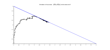
As illustrated in Figure1 ( X ¯ N ( t ) ) superscript ¯ 𝑋 𝑁 𝑡 (\bar{X}^{N}(t)) ( Y N ( t ) ) superscript 𝑌 𝑁 𝑡 (Y^{N}(t)) ( θ ¯ , ν N , A , R , 𝒮 ) ¯ 𝜃 superscript 𝜈 𝑁 𝐴 𝑅 𝒮 (\bar{\theta},\nu^{N},A,R,\mathcal{S})
V ¯ N ( t ) = X ¯ N ( 0 ) + M ¯ N ( t ) + t θ ¯ − ξ 𝒱 N ( t , Γ ) + ∫ 0 t A X ¯ N ( s ) 𝑑 s superscript ¯ 𝑉 𝑁 𝑡 superscript ¯ 𝑋 𝑁 0 superscript ¯ 𝑀 𝑁 𝑡 𝑡 ¯ 𝜃 𝜉 superscript 𝒱 𝑁 𝑡 Γ superscript subscript 0 𝑡 𝐴 superscript ¯ 𝑋 𝑁 𝑠 differential-d 𝑠 \bar{V}^{N}(t)=\bar{X}^{N}(0)+\bar{M}^{N}(t)+t\bar{\theta}-\xi\mathcal{V}^{N}(t,\Gamma)+\int_{0}^{t}A\bar{X}^{N}(s)ds (24)
Figure 1 :
In the next theorem we prove relative compactness of the sequence of processes
( X ¯ N ( . ) , Y N ( . ) , 𝒱 N ( . ) ) \left(\overline{X}^{N}(.),Y^{N}(.),\mathcal{V}^{N}(.)\right) 𝒟 ( ℝ + , ℝ 2 ) × ℳ 1 ( ℝ + × ℕ ¯ ) 𝒟 subscript ℝ superscript ℝ 2 subscript ℳ 1 subscript ℝ ¯ ℕ \mathcal{D}(\mathbb{R}_{+},\mathbb{R}^{2})\times\mathcal{M}_{1}(\mathbb{R}_{+}\times\bar{\mathbb{N}}) ℳ 1 ( ℝ + × ℕ ¯ ) subscript ℳ 1 subscript ℝ ¯ ℕ \mathcal{M}_{1}(\mathbb{R}_{+}\times\bar{\mathbb{N}}) ℝ + × ℕ ¯ subscript ℝ ¯ ℕ \mathbb{R}_{+}\times\bar{\mathbb{N}}
Theorem 3.2 .
Suppose that
l i m N → + ∞ ( X ¯ 1 N ( 0 ) , X ¯ 2 N ( 0 ) ) = ( x 1 , x 2 ) ∈ 𝒮 , → 𝑁 𝑙 𝑖 𝑚 superscript subscript ¯ 𝑋 1 𝑁 0 superscript subscript ¯ 𝑋 2 𝑁 0 subscript 𝑥 1 subscript 𝑥 2 𝒮 \displaystyle\underset{N\rightarrow+\infty}{lim}(\overline{X}_{1}^{N}(0),\overline{X}_{2}^{N}(0))=(x_{1},x_{2})\in\mathcal{S},
the sequence ( X ¯ N ( . ) , Y N ( . ) , ν N ( . ) ) \left(\overline{X}^{N}(.),Y^{N}(.),\nu^{N}(.)\right) 𝒟 ( ℝ + , ℝ 3 ) 𝒟 subscript ℝ superscript ℝ 3 \mathcal{D}(\mathbb{R}_{+},\mathbb{R}^{3}) ( x ( . ) , y ( . ) , ν ( . ) ) \left(x(.),y(.),\nu(.)\right)
x 1 ( t ) subscript 𝑥 1 𝑡 \displaystyle x_{1}(t) = x 1 − λ t − μ ∫ 0 t x 1 ( s ) 𝑑 s + 2 μ ∫ 0 t x 2 ( s ) 𝑑 s absent subscript 𝑥 1 𝜆 𝑡 𝜇 superscript subscript 0 𝑡 subscript 𝑥 1 𝑠 differential-d 𝑠 2 𝜇 superscript subscript 0 𝑡 subscript 𝑥 2 𝑠 differential-d 𝑠 \displaystyle=x_{1}-\lambda t-\mu\int_{0}^{t}x_{1}(s)ds+2\mu\int_{0}^{t}x_{2}(s)ds (25)
+ λ ∫ [ 0 , t ] × ℕ 𝟙 { x 1 ( s ) > 0 } 𝟙 { 0 } ( u ) ν ( d s × d u ) + λ y 1 ( t ) 𝜆 subscript 0 𝑡 ℕ subscript 1 subscript 𝑥 1 𝑠 0 subscript 1 0 𝑢 𝜈 𝑑 𝑠 𝑑 𝑢 𝜆 subscript 𝑦 1 𝑡 \displaystyle+\lambda\int_{[0,t]\times\mathbb{N}}\mathds{1}_{\{x_{1}(s)>0\}}\mathds{1}_{\{0\}}(u)\nu(ds\times du)+\lambda y_{1}(t)
x 2 ( t ) subscript 𝑥 2 𝑡 \displaystyle x_{2}(t) = x 2 + ( λ + ξ ) t − 2 μ ∫ 0 t x 2 ( s ) 𝑑 s − ξ ν ( [ 0 , t ] × { 0 , 1 } ) absent subscript 𝑥 2 𝜆 𝜉 𝑡 2 𝜇 superscript subscript 0 𝑡 subscript 𝑥 2 𝑠 differential-d 𝑠 𝜉 𝜈 0 𝑡 0 1 \displaystyle=x_{2}+(\lambda+\xi)t-2\mu\int_{0}^{t}x_{2}(s)ds-\xi\nu([0,t]\times\{0,1\}) (26)
− λ ∫ [ 0 , t ] × ℕ 𝟙 { x 1 ( s ) > 0 } 𝟙 { 0 } ( u ) ν ( d s × d u ) − λ y 1 ( t ) 𝜆 subscript 0 𝑡 ℕ subscript 1 subscript 𝑥 1 𝑠 0 subscript 1 0 𝑢 𝜈 𝑑 𝑠 𝑑 𝑢 𝜆 subscript 𝑦 1 𝑡 \displaystyle-\lambda\int_{[0,t]\times\mathbb{N}}\mathds{1}_{\{x_{1}(s)>0\}}\mathds{1}_{\{0\}}(u)\nu(ds\times du)-\lambda y_{1}(t)
where the function y 1 subscript 𝑦 1 y_{1} y 1 ( 0 ) = 0 subscript 𝑦 1 0 0 y_{1}(0)=0 t ≥ 0 𝑡 0 t\geq 0
y 1 ( t ) = ∫ 0 t 𝟙 { x 1 ( s ) = 0 } 𝑑 y 1 ( s ) subscript 𝑦 1 𝑡 superscript subscript 0 𝑡 subscript 1 subscript 𝑥 1 𝑠 0 differential-d subscript 𝑦 1 𝑠 \displaystyle y_{1}(t)=\int_{0}^{t}\mathds{1}_{\{x_{1}(s)=0\}}dy_{1}(s) (27)
Lemma 3.3 .
The sequences of processes ( M 1 N ( t ) N ) t ≥ 0 subscript superscript subscript 𝑀 1 𝑁 𝑡 𝑁 𝑡 0 (\frac{M_{1}^{N}(t)}{N})_{t\geq 0} ( M 2 N ( t ) N ) t ≥ 0 subscript superscript subscript 𝑀 2 𝑁 𝑡 𝑁 𝑡 0 (\frac{M_{2}^{N}(t)}{N})_{t\geq 0}
Proof.
Doob’s inequalities show that, for ϵ > 0 italic-ϵ 0 \epsilon>0 t ≥ 0 𝑡 0 t\geq 0
ℙ ( s u p 0 ≤ s ≤ t M i N ( s ) N ≥ ϵ ) ≤ 1 ϵ 2 N 2 𝔼 ( ⟨ M i N ⟩ ( t ) ) ℙ 0 𝑠 𝑡 𝑠 𝑢 𝑝 superscript subscript 𝑀 𝑖 𝑁 𝑠 𝑁 italic-ϵ 1 superscript italic-ϵ 2 superscript 𝑁 2 𝔼 delimited-⟨⟩ superscript subscript 𝑀 𝑖 𝑁 𝑡 \mathbb{P}\left(\underset{0\leq s\leq t}{sup}\frac{M_{i}^{N}(s)}{N}\geq\epsilon\right)\leq\frac{1}{\epsilon^{2}N^{2}}\mathbb{E}(\langle M_{i}^{N}\rangle(t))
From equations (11 12
𝔼 ( ⟨ M 1 N ⟩ ( t ) ) ≤ μ F N + λ N t 𝔼 ( ⟨ M 2 N ⟩ ( t ) ) ≤ μ F N + ( λ + ξ ) N t 𝔼 delimited-⟨⟩ superscript subscript 𝑀 1 𝑁 𝑡 𝜇 subscript 𝐹 𝑁 𝜆 𝑁 𝑡 𝔼 delimited-⟨⟩ superscript subscript 𝑀 2 𝑁 𝑡 𝜇 subscript 𝐹 𝑁 𝜆 𝜉 𝑁 𝑡 \begin{split}\mathbb{E}(\langle M_{1}^{N}\rangle(t))&\leq\mu F_{N}+\lambda Nt\\
\mathbb{E}(\langle M_{2}^{N}\rangle(t))&\leq\mu F_{N}+(\lambda+\xi)Nt\\
\end{split}
Then from (1 ( M 1 N ( t ) N ) t ≥ 0 subscript superscript subscript 𝑀 1 𝑁 𝑡 𝑁 𝑡 0 (\frac{M_{1}^{N}(t)}{N})_{t\geq 0} ( M 2 N ( t ) N ) t ≥ 0 subscript superscript subscript 𝑀 2 𝑁 𝑡 𝑁 𝑡 0 (\frac{M_{2}^{N}(t)}{N})_{t\geq 0}
proof of Theorem 3.2
First we prove the relative compactness of the process
X ¯ N ( t ) = ( X ¯ 1 N ( t ) X ¯ 2 N ( t ) ) superscript ¯ 𝑋 𝑁 𝑡 matrix superscript subscript ¯ 𝑋 1 𝑁 𝑡 superscript subscript ¯ 𝑋 2 𝑁 𝑡 \bar{X}^{N}(t)=\begin{pmatrix}\bar{X}_{1}^{N}(t)\\
\bar{X}_{2}^{N}(t)\end{pmatrix}
For this we prove separately that( X ¯ 1 N ( t ) ) superscript subscript ¯ 𝑋 1 𝑁 𝑡 (\overline{X}_{1}^{N}(t)) ( X ¯ 2 N ( t ) ) superscript subscript ¯ 𝑋 2 𝑁 𝑡 (\overline{X}_{2}^{N}(t))
For T > 0 , δ > 0 formulae-sequence 𝑇 0 𝛿 0 T>0,\delta>0 ω g T ( δ ) superscript subscript 𝜔 𝑔 𝑇 𝛿 \omega_{g}^{T}(\delta) [ 0 , T ] 0 𝑇 [0,T]
ω g T ( δ ) = sup 0 ≤ s ≤ t ≤ T , | t − s | ≤ δ | g ( t ) − g ( s ) | superscript subscript 𝜔 𝑔 𝑇 𝛿 subscript supremum formulae-sequence 0 𝑠 𝑡 𝑇 𝑡 𝑠 𝛿 𝑔 𝑡 𝑔 𝑠 \omega_{g}^{T}(\delta)=\sup_{0\leq s\leq t\leq T,|t-s|\leq\delta}|g(t)-g(s)| (28)
The equation (21 ( X ¯ 1 N ( t ) , Y 1 N ( t ) ) superscript subscript ¯ 𝑋 1 𝑁 𝑡 superscript subscript 𝑌 1 𝑁 𝑡 (\overline{X}_{1}^{N}(t),Y_{1}^{N}(t)) Y 1 N ( t ) = λ ∫ 0 t 𝟙 { X 1 N ( u ) = 0 } d u ) Y_{1}^{N}(t)=\lambda\int_{0}^{t}\mathds{1}_{\{X_{1}^{N}(u)=0\}}du)
V ¯ 1 N ( t ) superscript subscript ¯ 𝑉 1 𝑁 𝑡 \displaystyle\overline{V}_{1}^{N}(t) = X ¯ 1 N ( 0 ) + M ¯ 1 N ( t ) − λ t + μ ∫ 0 t ( 2 X ¯ 2 N ( u ) − X ¯ 1 N ( u ) ) 𝑑 u absent superscript subscript ¯ 𝑋 1 𝑁 0 superscript subscript ¯ 𝑀 1 𝑁 𝑡 𝜆 𝑡 𝜇 superscript subscript 0 𝑡 2 superscript subscript ¯ 𝑋 2 𝑁 𝑢 superscript subscript ¯ 𝑋 1 𝑁 𝑢 differential-d 𝑢 \displaystyle=\overline{X}_{1}^{N}(0)+\overline{M}_{1}^{N}(t)-\lambda t+\mu\int_{0}^{t}(2\overline{X}_{2}^{N}(u)-\overline{X}_{1}^{N}(u))du (29)
+ λ ∫ [ 0 , t ] × ℕ 𝟙 { X 1 N ( u ) > 0 } 𝟙 { 0 } ( y ) ν N ( d s × d y ) 𝜆 subscript 0 𝑡 ℕ subscript 1 superscript subscript 𝑋 1 𝑁 𝑢 0 subscript 1 0 𝑦 superscript 𝜈 𝑁 𝑑 𝑠 𝑑 𝑦 \displaystyle+\lambda\int_{[0,t]\times\mathbb{N}}\mathds{1}_{\{{X_{1}}^{N}(u)>0\}}\mathds{1}_{\{0\}}(y)\nu^{N}(ds\times dy)
By using explicit representation of the solution of the Skorokhod in dimension 1 [3 ] , one has
‖ X ¯ 1 N ‖ ∞ , t = d e f sup 0 ≤ s ≤ t | X ¯ 1 N ( s ) | ≤ 2 ‖ V ¯ 1 N ‖ ∞ , t superscript 𝑑 𝑒 𝑓 subscript norm superscript subscript ¯ 𝑋 1 𝑁 𝑡
subscript supremum 0 𝑠 𝑡 superscript subscript ¯ 𝑋 1 𝑁 𝑠 2 subscript norm superscript subscript ¯ 𝑉 1 𝑁 𝑡
\|\overline{X}_{1}^{N}\|_{\infty,t}\stackrel{{\scriptstyle def}}{{=}}\sup_{0\leq s\leq t}|\overline{X}_{1}^{N}(s)|\leq 2\|\overline{V}_{1}^{N}\|_{\infty,t}
and
| λ Y 1 N ( t ) | ≤ ‖ V ¯ 1 N ‖ ∞ , t 𝜆 superscript subscript 𝑌 1 𝑁 𝑡 subscript norm superscript subscript ¯ 𝑉 1 𝑁 𝑡
|\lambda Y_{1}^{N}(t)|\leq\|\overline{V}_{1}^{N}\|_{\infty,t}
By equation (29
‖ V ¯ 1 N ‖ ∞ , t subscript norm superscript subscript ¯ 𝑉 1 𝑁 𝑡
\displaystyle\|\overline{V}_{1}^{N}\|_{\infty,t} ≤ | X ¯ 1 N ( 0 ) ) | + 2 λ t + μ ∫ 0 t ∥ X ¯ 1 N ∥ ∞ , s d s \displaystyle\leq|\overline{X}_{1}^{N}(0))|+2\lambda t+\mu\int_{0}^{t}\|\overline{X}_{1}^{N}\|_{\infty,s}ds
+ 2 μ ∫ 0 t ‖ X ¯ 2 N ‖ ∞ , s 𝑑 s + ‖ M ¯ 1 N ‖ ∞ , t 2 𝜇 superscript subscript 0 𝑡 subscript norm superscript subscript ¯ 𝑋 2 𝑁 𝑠
differential-d 𝑠 subscript norm superscript subscript ¯ 𝑀 1 𝑁 𝑡
\displaystyle+2\mu\int_{0}^{t}\|\overline{X}_{2}^{N}\|_{\infty,s}ds+\|\overline{M}_{1}^{N}\|_{\infty,t}
and using inequalities given above,
‖ X ¯ 1 N ‖ ∞ , t subscript norm superscript subscript ¯ 𝑋 1 𝑁 𝑡
\displaystyle\|\overline{X}_{1}^{N}\|_{\infty,t} ≤ 2 | X ¯ 1 N ( 0 ) | + 4 λ t + 2 μ ∫ 0 t ‖ X ¯ 1 N ‖ ∞ , s 𝑑 s absent 2 superscript subscript ¯ 𝑋 1 𝑁 0 4 𝜆 𝑡 2 𝜇 superscript subscript 0 𝑡 subscript norm superscript subscript ¯ 𝑋 1 𝑁 𝑠
differential-d 𝑠 \displaystyle\leq 2|\overline{X}_{1}^{N}(0)|+4\lambda t+2\mu\int_{0}^{t}\|\overline{X}_{1}^{N}\|_{\infty,s}ds
+ 4 μ ∫ 0 t ‖ X ¯ 2 N ‖ ∞ , s 𝑑 s + 2 ‖ M ¯ 1 N ‖ ∞ , t 4 𝜇 superscript subscript 0 𝑡 subscript norm superscript subscript ¯ 𝑋 2 𝑁 𝑠
differential-d 𝑠 2 subscript norm superscript subscript ¯ 𝑀 1 𝑁 𝑡
\displaystyle+4\mu\int_{0}^{t}\|\overline{X}_{2}^{N}\|_{\infty,s}ds+2\|\overline{M}_{1}^{N}\|_{\infty,t}
‖ X ¯ 2 N ‖ ∞ , t subscript norm superscript subscript ¯ 𝑋 2 𝑁 𝑡
\displaystyle\|\overline{X}_{2}^{N}\|_{\infty,t} ≤ | X ¯ 1 N ( 0 ) | + | X ¯ 2 N ( 0 ) | + ( 4 λ + 3 ξ ) t + ‖ M ¯ 1 N ‖ ∞ , t + ‖ M ¯ 2 N ‖ ∞ , t absent superscript subscript ¯ 𝑋 1 𝑁 0 superscript subscript ¯ 𝑋 2 𝑁 0 4 𝜆 3 𝜉 𝑡 subscript norm superscript subscript ¯ 𝑀 1 𝑁 𝑡
subscript norm superscript subscript ¯ 𝑀 2 𝑁 𝑡
\displaystyle\leq|\overline{X}_{1}^{N}(0)|+|\overline{X}_{2}^{N}(0)|+(4\lambda+3\xi)t+\|\overline{M}_{1}^{N}\|_{\infty,t}+\|\overline{M}_{2}^{N}\|_{\infty,t}
+ μ ∫ 0 t ‖ X ¯ 1 N ‖ ∞ , s 𝑑 s + 4 μ ∫ 0 t ‖ X ¯ 2 N ‖ ∞ , s 𝑑 s 𝜇 superscript subscript 0 𝑡 subscript norm superscript subscript ¯ 𝑋 1 𝑁 𝑠
differential-d 𝑠 4 𝜇 superscript subscript 0 𝑡 subscript norm superscript subscript ¯ 𝑋 2 𝑁 𝑠
differential-d 𝑠 \displaystyle+\mu\int_{0}^{t}\|\overline{X}_{1}^{N}\|_{\infty,s}ds+4\mu\int_{0}^{t}\|\overline{X}_{2}^{N}\|_{\infty,s}ds
Then
‖ X ¯ 1 N ‖ ∞ , t + ‖ X ¯ 2 N ‖ ∞ , t ≤ H N ( T ) + 8 μ ∫ 0 t ( ‖ X ¯ 1 N ‖ ∞ , s + ‖ X ¯ 2 N ‖ ∞ , s ) 𝑑 s subscript norm superscript subscript ¯ 𝑋 1 𝑁 𝑡
subscript norm superscript subscript ¯ 𝑋 2 𝑁 𝑡
superscript 𝐻 𝑁 𝑇 8 𝜇 superscript subscript 0 𝑡 subscript norm superscript subscript ¯ 𝑋 1 𝑁 𝑠
subscript norm superscript subscript ¯ 𝑋 2 𝑁 𝑠
differential-d 𝑠 \|\overline{X}_{1}^{N}\|_{\infty,t}+\|\overline{X}_{2}^{N}\|_{\infty,t}\leq H^{N}(T)+8\mu\int_{0}^{t}(\|\overline{X}_{1}^{N}\|_{\infty,s}+\|\overline{X}_{2}^{N}\|_{\infty,s})ds
with
H N ( t ) = 3 | X ¯ 1 N ( 0 ) | + | X ¯ 2 N ( 0 ) | + ( 8 λ + 3 ξ ) T + 3 ‖ M ¯ 1 N ‖ ∞ , T + ‖ M ¯ 2 N ‖ ∞ , T superscript 𝐻 𝑁 𝑡 3 superscript subscript ¯ 𝑋 1 𝑁 0 superscript subscript ¯ 𝑋 2 𝑁 0 8 𝜆 3 𝜉 𝑇 3 subscript norm superscript subscript ¯ 𝑀 1 𝑁 𝑇
subscript norm superscript subscript ¯ 𝑀 2 𝑁 𝑇
H^{N}(t)=3|\overline{X}_{1}^{N}(0)|+|\overline{X}_{2}^{N}(0)|+(8\lambda+3\xi)T+3\|\overline{M}_{1}^{N}\|_{\infty,T}+\|\overline{M}_{2}^{N}\|_{\infty,T}
Gronwall’s lemma gives that the relation
‖ X ¯ 1 N ‖ ∞ , t + ‖ X ¯ 2 N ‖ ∞ , t ≤ H N ( T ) e 8 μ t subscript norm superscript subscript ¯ 𝑋 1 𝑁 𝑡
subscript norm superscript subscript ¯ 𝑋 2 𝑁 𝑡
superscript 𝐻 𝑁 𝑇 superscript 𝑒 8 𝜇 𝑡 \|\overline{X}_{1}^{N}\|_{\infty,t}+\|\overline{X}_{2}^{N}\|_{\infty,t}\leq H^{N}(T)e^{8\mu t}
holds for all t ∈ [ 0 , T ] 𝑡 0 𝑇 t\in[0,T] | X ¯ 1 N ( 0 ) | superscript subscript ¯ 𝑋 1 𝑁 0 |\overline{X}_{1}^{N}(0)| | X ¯ 2 N ( 0 ) | superscript subscript ¯ 𝑋 2 𝑁 0 |\overline{X}_{2}^{N}(0)| ( H N ( T ) ) superscript 𝐻 𝑁 𝑇 (H^{N}(T)) ϵ > 0 italic-ϵ 0 \epsilon>0 C > 0 𝐶 0 C>0 i = 1 , 2 𝑖 1 2
i=1,2 N ∈ ℕ 𝑁 ℕ N\in\mathbb{N}
ℙ ( ‖ X ¯ 1 N ‖ ∞ , t + ‖ X ¯ 2 N ‖ ∞ , t > C ) ≤ ϵ . ℙ subscript norm superscript subscript ¯ 𝑋 1 𝑁 𝑡
subscript norm superscript subscript ¯ 𝑋 2 𝑁 𝑡
𝐶 italic-ϵ \mathbb{P}\left(\|\overline{X}_{1}^{N}\|_{\infty,t}+\|\overline{X}_{2}^{N}\|_{\infty,t}>C\right)\leq\epsilon.
If η > 0 𝜂 0 \eta>0 N 1 subscript 𝑁 1 N_{1} δ > 0 𝛿 0 \delta>0 N ≥ N 1 𝑁 subscript 𝑁 1 N\geq N_{1}
δ ( λ + 4 μ C ) ≤ η 2 𝛿 𝜆 4 𝜇 𝐶 𝜂 2 \delta(\lambda+4\mu C)\leq\frac{\eta}{2}
and
ℙ ( ω M ¯ 1 N T ( δ ) ≥ η 2 ) ≤ ϵ ℙ superscript subscript 𝜔 superscript subscript ¯ 𝑀 1 𝑁 𝑇 𝛿 𝜂 2 italic-ϵ \mathbb{P}\left(\omega_{\overline{M}_{1}^{N}}^{T}(\delta)\geq\frac{\eta}{2}\right)\leq\epsilon
One gets finally
ℙ ( ω V ¯ 1 N T ( δ ) ≥ η ) ℙ superscript subscript 𝜔 superscript subscript ¯ 𝑉 1 𝑁 𝑇 𝛿 𝜂 \displaystyle\mathbb{P}\left(\omega_{\overline{V}_{1}^{N}}^{T}(\delta)\geq\eta\right) ≤ ℙ ( 2 λ δ + 2 μ δ ( ‖ X ¯ 1 N ‖ ∞ , T + ‖ X ¯ 2 N ‖ ∞ , T ) ≥ η 2 ) absent ℙ 2 𝜆 𝛿 2 𝜇 𝛿 subscript norm superscript subscript ¯ 𝑋 1 𝑁 𝑇
subscript norm superscript subscript ¯ 𝑋 2 𝑁 𝑇
𝜂 2 \displaystyle\leq\mathbb{P}\left(2\lambda\delta+2\mu\delta(\|\overline{X}_{1}^{N}\|_{\infty,T}+\|\overline{X}_{2}^{N}\|_{\infty,T})\geq\frac{\eta}{2}\right)
+ ℙ ( ω M ¯ 1 N T ( δ ) ≥ η 2 ) ≤ 3 ϵ ℙ superscript subscript 𝜔 superscript subscript ¯ 𝑀 1 𝑁 𝑇 𝛿 𝜂 2 3 italic-ϵ \displaystyle+\mathbb{P}\left(\omega_{\overline{M}_{1}^{N}}^{T}(\delta)\geq\frac{\eta}{2}\right)\leq 3\epsilon
Consequently the sequence ( V ¯ 1 N ( t ) ) superscript subscript ¯ 𝑉 1 𝑁 𝑡 (\overline{V}_{1}^{N}(t)) ( X ¯ 1 N ( t ) ) superscript subscript ¯ 𝑋 1 𝑁 𝑡 (\overline{X}_{1}^{N}(t)) ( Y ¯ 1 N ( t ) ) superscript subscript ¯ 𝑌 1 𝑁 𝑡 (\overline{Y}_{1}^{N}(t)) [1 ] .
From equation ((22 s < t 𝑠 𝑡 s<t
| X ¯ 2 N ( t ) − X ¯ 2 N ( s ) | superscript subscript ¯ 𝑋 2 𝑁 𝑡 superscript subscript ¯ 𝑋 2 𝑁 𝑠 \displaystyle|\overline{X}_{2}^{N}(t)-\overline{X}_{2}^{N}(s)| ≤ ( λ + ξ ) ( t − s ) + 2 μ ∫ s t | X ¯ 2 N ( u ) | 𝑑 u + | M ¯ 2 N ( t ) − M ¯ 2 N ( s ) | absent 𝜆 𝜉 𝑡 𝑠 2 𝜇 superscript subscript 𝑠 𝑡 superscript subscript ¯ 𝑋 2 𝑁 𝑢 differential-d 𝑢 superscript subscript ¯ 𝑀 2 𝑁 𝑡 superscript subscript ¯ 𝑀 2 𝑁 𝑠 \displaystyle\leq(\lambda+\xi)(t-s)+2\mu\int_{s}^{t}|\overline{X}_{2}^{N}(u)|du+|\overline{M}_{2}^{N}(t)-\overline{M}_{2}^{N}(s)|
+ ( 2 λ + ξ ) ( t − s ) + λ ( Y 1 N ( t ) − Y 1 N ( s ) ) 2 𝜆 𝜉 𝑡 𝑠 𝜆 superscript subscript 𝑌 1 𝑁 𝑡 superscript subscript 𝑌 1 𝑁 𝑠 \displaystyle+(2\lambda+\xi)(t-s)+\lambda(Y_{1}^{N}(t)-Y_{1}^{N}(s))
and
ℙ ( ω X ¯ 2 N T ( δ ) ≥ η ) ℙ superscript subscript 𝜔 superscript subscript ¯ 𝑋 2 𝑁 𝑇 𝛿 𝜂 \displaystyle\mathbb{P}\left(\omega_{\overline{X}_{2}^{N}}^{T}(\delta)\geq\eta\right) ≤ ℙ ( ω M ¯ 2 N T ( δ ) ≥ η / 3 ) + ℙ ( ω Y 1 N T ( δ ) ≥ η / 3 ) absent ℙ superscript subscript 𝜔 superscript subscript ¯ 𝑀 2 𝑁 𝑇 𝛿 𝜂 3 ℙ superscript subscript 𝜔 superscript subscript 𝑌 1 𝑁 𝑇 𝛿 𝜂 3 \displaystyle\leq\mathbb{P}\left(\omega_{\overline{M}_{2}^{N}}^{T}(\delta)\geq\eta/3\right)+\mathbb{P}\left(\omega_{Y_{1}^{N}}^{T}(\delta)\geq\eta/3\right) (30)
+ ℙ ( 2 μ δ ‖ X ¯ 2 N ‖ ∞ , T + δ ( 2 λ + 3 ξ ) ≥ η / 3 ) ℙ 2 𝜇 𝛿 subscript norm superscript subscript ¯ 𝑋 2 𝑁 𝑇
𝛿 2 𝜆 3 𝜉 𝜂 3 \displaystyle+\mathbb{P}\left(2\mu\delta\|\overline{X}_{2}^{N}\|_{\infty,T}+\delta(2\lambda+3\xi)\geq\eta/3\right)
There exists N 1 ≥ 0 subscript 𝑁 1 0 N_{1}\geq 0 δ ( 2 μ C − ξ ) ≤ ϵ 𝛿 2 𝜇 𝐶 𝜉 italic-ϵ \delta(2\mu C-\xi)\leq\epsilon
ℙ ( ω M ¯ 2 N T ( δ ) ≥ η 3 ) ≤ ϵ ℙ superscript subscript 𝜔 superscript subscript ¯ 𝑀 2 𝑁 𝑇 𝛿 𝜂 3 italic-ϵ \mathbb{P}\left(\omega_{\overline{M}_{2}^{N}}^{T}(\delta)\geq\frac{\eta}{3}\right)\leq\epsilon
and
ℙ ( λ ω Y 1 N N T ( δ ) ≥ η 3 ) ≤ ϵ ℙ 𝜆 superscript subscript 𝜔 superscript subscript 𝑌 1 𝑁 𝑁 𝑇 𝛿 𝜂 3 italic-ϵ \mathbb{P}\left(\lambda\omega_{\frac{Y_{1}^{N}}{N}}^{T}(\delta)\geq\frac{\eta}{3}\right)\leq\epsilon
and, consequently
ℙ ( ω X ¯ 2 N T ( δ ) ≥ η ) ≤ 3 ϵ ℙ superscript subscript 𝜔 superscript subscript ¯ 𝑋 2 𝑁 𝑇 𝛿 𝜂 3 italic-ϵ \mathbb{P}\left(\omega_{\overline{X}_{2}^{N}}^{T}(\delta)\geq\eta\right)\leq 3\epsilon
The sequence X ¯ 2 N superscript subscript ¯ 𝑋 2 𝑁 \overline{X}_{2}^{N}
It remains to prove relative compactness of the sequence of random measures ν N superscript 𝜈 𝑁 \nu^{N} [ 0 , + ∞ [ × ℕ ¯ [0,+\infty[\times\bar{\mathbb{N}} N 𝑁 N t ≥ 0 𝑡 0 t\geq 0
ν N ( [ 0 , t [ × ℕ ¯ ) = t \nu^{N}([0,t[\times\bar{\mathbb{N}})=t
The result is given in [9 ] Lemma 1.3.
∎
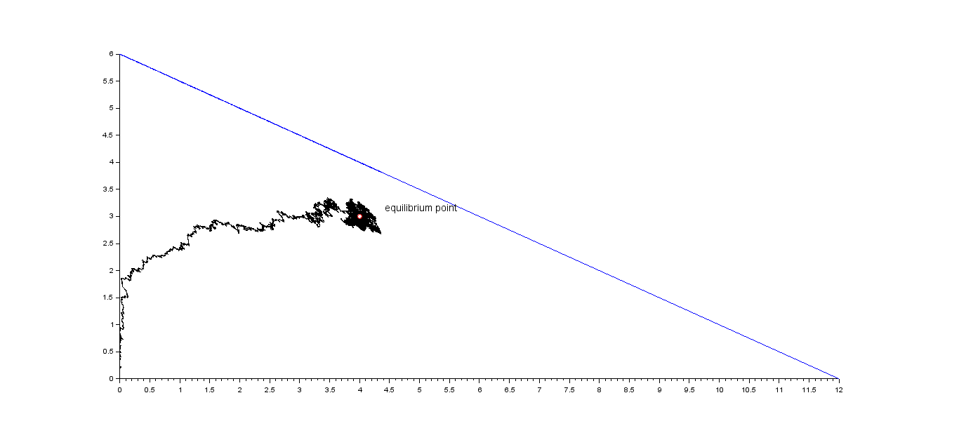
4 The under-loaded regime
Throughout this section, we assume that the condition
ρ < β ¯ 𝜌 ¯ 𝛽 \rho<\bar{\beta} (34)
holds.
Figure 2 : The under-load regime
Let ( X 1 N ( t ) ) superscript subscript 𝑋 1 𝑁 𝑡 (X_{1}^{N}(t)) ( X 2 N ( t ) ) superscript subscript 𝑋 2 𝑁 𝑡 (X_{2}^{N}(t)) 7 8 ( X 1 N ( t ) + X 2 N ( t ) ) superscript subscript 𝑋 1 𝑁 𝑡 superscript subscript 𝑋 2 𝑁 𝑡 (X_{1}^{N}(t)+X_{2}^{N}(t)) t 𝑡 t ( Z N ( t ) ) superscript 𝑍 𝑁 𝑡 (Z^{N}(t))
Z N ( t ) = X 1 N ( t ) + 2 X 2 N ( t ) − N ρ N superscript 𝑍 𝑁 𝑡 superscript subscript 𝑋 1 𝑁 𝑡 2 superscript subscript 𝑋 2 𝑁 𝑡 𝑁 𝜌 𝑁 Z^{N}(t)=\dfrac{X_{1}^{N}(t)+2X_{2}^{N}(t)-N\rho}{\sqrt{N}} (35)
The Q-matrix Q N = ( q N ( . , . ) ) Q^{N}=(q^{N}(.,.)) ( X 1 N ( t ) , X 2 N ( t ) , Z N ( t ) ) superscript subscript 𝑋 1 𝑁 𝑡 superscript subscript 𝑋 2 𝑁 𝑡 superscript 𝑍 𝑁 𝑡 (X_{1}^{N}(t),X_{2}^{N}(t),Z^{N}(t))
For ( x 1 , x 2 ) ∈ 𝒟 N subscript 𝑥 1 subscript 𝑥 2 superscript 𝒟 𝑁 (x_{1},x_{2})\in\mathcal{D}^{N} z = x 1 + 2 x 2 − N ρ N 𝑧 subscript 𝑥 1 2 subscript 𝑥 2 𝑁 𝜌 𝑁 z=\dfrac{x_{1}+2x_{2}-N\rho}{\sqrt{N}}
( x 1 , x 2 , z ) ⟶ ( x 1 , x 2 , z ) + { ( 0 , 1 , 2 N ) ξ N 𝟙 { z < F N − 1 N − N ρ } ( 1 , − 1 , − 1 N ) 2 μ x 2 ( − 1 , 1 , 1 N ) λ N 𝟙 { x 1 > 0 , z < F N N − N ρ } ( − 1 , 0 , − 1 N ) μ x 1 ⟶ subscript 𝑥 1 subscript 𝑥 2 𝑧 subscript 𝑥 1 subscript 𝑥 2 𝑧 cases 0 1 2 𝑁 𝜉 𝑁 subscript 1 𝑧 subscript 𝐹 𝑁 1 𝑁 𝑁 𝜌
missing-subexpression 1 1 1 𝑁 2 𝜇 subscript 𝑥 2 missing-subexpression 1 1 1 𝑁 𝜆 𝑁 subscript 1 formulae-sequence subscript 𝑥 1 0 𝑧 subscript 𝐹 𝑁 𝑁 𝑁 𝜌
missing-subexpression 1 0 1 𝑁 𝜇 subscript 𝑥 1
missing-subexpression (x_{1},x_{2},z)\longrightarrow(x_{1},x_{2},z)+\left\{\begin{array}[]{ll}(0,1,\frac{2}{\sqrt{N}})\ \ \xi N\mathds{1}_{\{z<\frac{F_{N}-1}{\sqrt{N}}-N\rho\}}\\
(1,-1,-\frac{1}{\sqrt{N}})\ \ 2\mu x_{2}\\
(-1,1,\frac{1}{\sqrt{N}})\ \ \lambda N\mathds{1}_{\{x_{1}>0,z<\frac{F_{N}}{\sqrt{N}}-N\rho\}}\\
(-1,0,-\frac{1}{\sqrt{N}})\ \ \mu x_{1}\end{array}\right. (36)
and the generator of ( X 1 N ( t ) , X 2 N ( t ) , Z N ( t ) ) superscript subscript 𝑋 1 𝑁 𝑡 superscript subscript 𝑋 2 𝑁 𝑡 superscript 𝑍 𝑁 𝑡 (X_{1}^{N}(t),X_{2}^{N}(t),Z^{N}(t))
A N f ( x 1 , x 2 , z ) superscript 𝐴 𝑁 𝑓 subscript 𝑥 1 subscript 𝑥 2 𝑧 \displaystyle A^{N}f(x_{1},x_{2},z) = ξ N 𝟙 { z < F N − N ρ − 1 N } [ f ( x 1 , x 2 + 1 , z + 2 N ) − f ( x 1 , x 2 , z ) ] absent 𝜉 𝑁 subscript 1 𝑧 subscript 𝐹 𝑁 𝑁 𝜌 1 𝑁 delimited-[] 𝑓 subscript 𝑥 1 subscript 𝑥 2 1 𝑧 2 𝑁 𝑓 subscript 𝑥 1 subscript 𝑥 2 𝑧 \displaystyle=\xi N\mathds{1}_{\{z<\frac{F_{N}-N\rho-1}{\sqrt{N}}\}}[f(x_{1},x_{2}+1,z+\frac{2}{\sqrt{N}})-f(x_{1},x_{2},z)]
+ λ N 𝟙 { x 1 > 0 , z < F N − N ρ N } [ f ( x 1 − 1 , x 2 + 1 , z + 1 N ) − f ( x 1 , x 2 , z ) ] 𝜆 𝑁 subscript 1 formulae-sequence subscript 𝑥 1 0 𝑧 subscript 𝐹 𝑁 𝑁 𝜌 𝑁 delimited-[] 𝑓 subscript 𝑥 1 1 subscript 𝑥 2 1 𝑧 1 𝑁 𝑓 subscript 𝑥 1 subscript 𝑥 2 𝑧 \displaystyle+\lambda N\mathds{1}_{\{x_{1}>0\ ,\ z<\frac{F_{N}-N\rho}{\sqrt{N}}\}}[f(x_{1}-1,x_{2}+1,z+\frac{1}{\sqrt{N}})-f(x_{1},x_{2},z)]
+ μ x 1 [ f ( x 1 − 1 , x 2 , z − 1 N ) − f ( x 1 , x 2 , z ) ] 𝜇 subscript 𝑥 1 delimited-[] 𝑓 subscript 𝑥 1 1 subscript 𝑥 2 𝑧 1 𝑁 𝑓 subscript 𝑥 1 subscript 𝑥 2 𝑧 \displaystyle+\mu x_{1}[f(x_{1}-1,x_{2},z-\frac{1}{\sqrt{N}})-f(x_{1},x_{2},z)]
+ 2 μ x 2 [ f ( x 1 + 1 , x 2 − 1 , z − 1 N ) − f ( x 1 , x 2 , z ) ] 2 𝜇 subscript 𝑥 2 delimited-[] 𝑓 subscript 𝑥 1 1 subscript 𝑥 2 1 𝑧 1 𝑁 𝑓 subscript 𝑥 1 subscript 𝑥 2 𝑧 \displaystyle+2\mu x_{2}[f(x_{1}+1,x_{2}-1,z-\frac{1}{\sqrt{N}})-f(x_{1},x_{2},z)]
For any function f 𝑓 f z 𝑧 z
f ( x 1 , x 2 , z ) = g ( z ) ∀ ( x 1 , x 2 ) ∈ ℕ 2 with x 1 > 0 formulae-sequence 𝑓 subscript 𝑥 1 subscript 𝑥 2 𝑧 𝑔 𝑧 formulae-sequence for-all subscript 𝑥 1 subscript 𝑥 2 superscript ℕ 2 with
subscript 𝑥 1 0 f(x_{1},x_{2},z)=g(z)\quad\forall\;(x_{1},x_{2})\in\mathbb{N}^{2}\quad\textit{with}\quad x_{1}>0
for some twice differentiable function g 𝑔 g ℝ ℝ \mathbb{R}
A N g ( z ) superscript 𝐴 𝑁 𝑔 𝑧 \displaystyle A^{N}g(z) = ξ N 𝟙 { z < F N − N ρ − 1 N } [ g ( z + 2 N ) − g ( z ) ] absent 𝜉 𝑁 subscript 1 𝑧 subscript 𝐹 𝑁 𝑁 𝜌 1 𝑁 delimited-[] 𝑔 𝑧 2 𝑁 𝑔 𝑧 \displaystyle=\xi N\mathds{1}_{\{z<\frac{F_{N}-N\rho-1}{\sqrt{N}}\}}[g(z+\frac{2}{\sqrt{N}})-g(z)]
+ λ N 𝟙 { z < F N − N ρ N } [ g ( z + 1 N ) − g ( z ) ] 𝜆 𝑁 subscript 1 𝑧 subscript 𝐹 𝑁 𝑁 𝜌 𝑁 delimited-[] 𝑔 𝑧 1 𝑁 𝑔 𝑧 \displaystyle+\lambda N\mathds{1}_{\{z<\frac{F_{N}-N\rho}{\sqrt{N}}\}}[g(z+\frac{1}{\sqrt{N}})-g(z)]
+ μ ( N z + N ρ ) [ g ( z − 1 N ) − g ( z ) ] 𝜇 𝑁 𝑧 𝑁 𝜌 delimited-[] 𝑔 𝑧 1 𝑁 𝑔 𝑧 \displaystyle+\mu(\sqrt{N}z+N\rho)[g(z-\frac{1}{\sqrt{N}})-g(z)]
Remark that condition (34 F N − N ρ − 1 N subscript 𝐹 𝑁 𝑁 𝜌 1 𝑁 \frac{F_{N}-N\rho-1}{\sqrt{N}} F N − N ρ N subscript 𝐹 𝑁 𝑁 𝜌 𝑁 \frac{F_{N}-N\rho}{\sqrt{N}} + ∞ +\infty
− μ z g ′ ( z ) + ( λ + 3 ξ ) g ′′ ( z ) z ∈ ℝ 𝜇 𝑧 superscript 𝑔 ′ 𝑧 𝜆 3 𝜉 superscript 𝑔 ′′ 𝑧 𝑧
ℝ -\mu zg^{\prime}(z)+(\lambda+3\xi)g^{\prime\prime}(z)\qquad z\in\mathbb{R}
when N → + ∞ → 𝑁 N\rightarrow+\infty λ + 3 ξ μ 𝜆 3 𝜉 𝜇 \frac{\lambda+3\xi}{\mu} [5 ] one can see that for some positive constant α 𝛼 \alpha ( X 1 N ( t ) + 2 X 2 N ( t ) ) superscript subscript 𝑋 1 𝑁 𝑡 2 superscript subscript 𝑋 2 𝑁 𝑡 (X_{1}^{N}(t)+2X_{2}^{N}(t)) [ N ρ − α N , N ρ + α N ] ⊂ [ 0 , N β ¯ ] 𝑁 𝜌 𝛼 𝑁 𝑁 𝜌 𝛼 𝑁 0 𝑁 ¯ 𝛽 [N\rho-\alpha N,N\rho+\alpha N]\subset[0,N\bar{\beta}] F N = + ∞ subscript 𝐹 𝑁 F_{N}=+\infty ( X 1 N ( t ) , X 2 N ( t ) ) superscript subscript 𝑋 1 𝑁 𝑡 superscript subscript 𝑋 2 𝑁 𝑡 (X_{1}^{N}(t),X_{2}^{N}(t)) [4 ] .
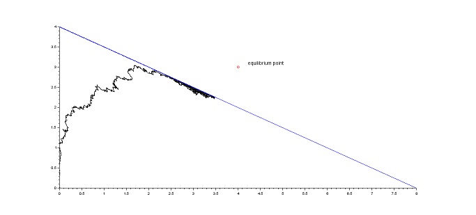
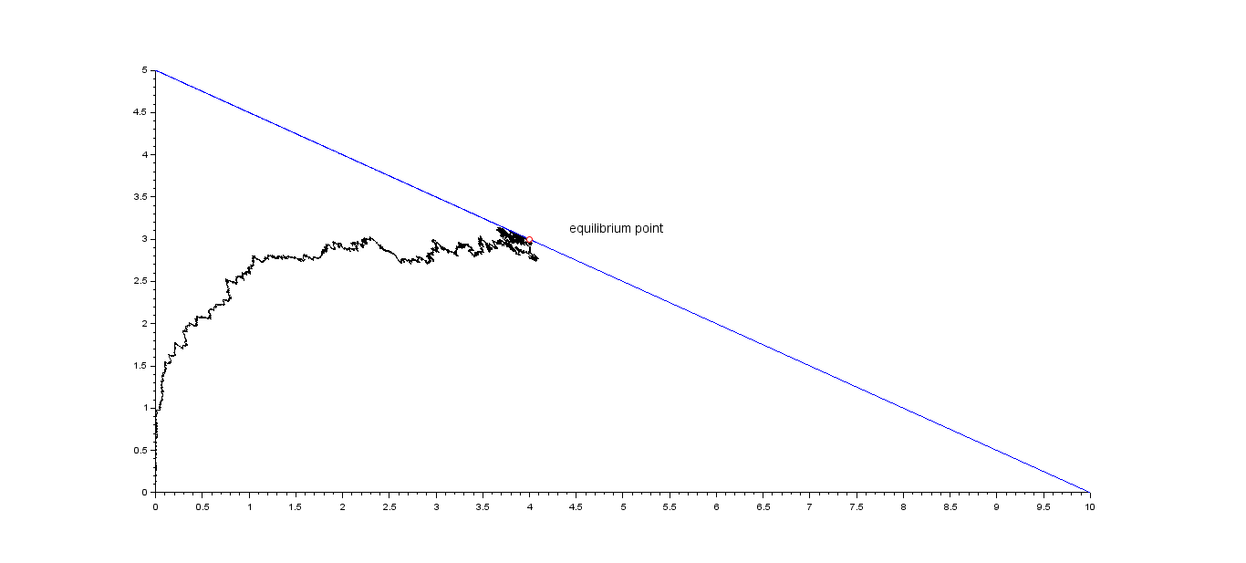
5 The overloaded regime
Throughout this section, we assume that the condition
ρ > β ¯ 𝜌 ¯ 𝛽 \rho>\bar{\beta} (37)
holds.
Figure 3 : The overload regime
the Q-matrix Q N = ( q N ( . , . ) ) Q^{N}=(q^{N}(.,.)) ( X 1 N ( t / N ) , X 2 N ( t / N ) , m N ( t / N ) ) superscript subscript 𝑋 1 𝑁 𝑡 𝑁 superscript subscript 𝑋 2 𝑁 𝑡 𝑁 superscript 𝑚 𝑁 𝑡 𝑁 ({X_{1}}^{N}(t/N),{X_{2}}^{N}(t/N),m^{N}(t/N))
{ q N ( ( x 1 , x 2 , m ) , ( x 1 − 1 , x 2 , m + 1 ) = 1 N μ x 1 q N ( ( x 1 , x 2 , m ) , ( x 1 + 1 , x 2 − 1 , m + 1 ) = 2 N μ x 2 q N ( ( x 1 , x 2 , m ) , ( x 1 − 1 , x 2 + 1 , m − 1 ) = λ 𝟙 { x 1 > 0 , m ≥ 1 } q N ( ( x 1 , x 2 , m ) , ( x 1 , x 2 + 1 , m − 2 ) = ξ 𝟙 { m ≥ 2 } \left\{\begin{array}[]{ll}q^{N}((x_{1},x_{2},m),(x_{1}-1,x_{2},m+1)=\frac{1}{N}\mu x_{1}\\
q^{N}((x_{1},x_{2},m),(x_{1}+1,x_{2}-1,m+1)=\frac{2}{N}\mu x_{2}\\
q^{N}((x_{1},x_{2},m),(x_{1}-1,x_{2}+1,m-1)=\lambda\mathds{1}_{\{x_{1}>0\ ,\ m\geq 1\}}\\
q^{N}((x_{1},x_{2},m),(x_{1},x_{2}+1,m-2)=\xi\mathds{1}_{\{m\geq 2\}}\end{array}\right.
A N f ( x 1 , x 2 , m ) subscript 𝐴 𝑁 𝑓 subscript 𝑥 1 subscript 𝑥 2 𝑚 \displaystyle A_{N}f(x_{1},x_{2},m) = 1 N μ x 1 [ f ( x 1 − 1 , x 2 , m + 1 ) − f ( x 1 , x 2 , m ) ] absent 1 𝑁 𝜇 subscript 𝑥 1 delimited-[] 𝑓 subscript 𝑥 1 1 subscript 𝑥 2 𝑚 1 𝑓 subscript 𝑥 1 subscript 𝑥 2 𝑚 \displaystyle=\frac{1}{N}\mu x_{1}[f(x_{1}-1,x_{2},m+1)-f(x_{1},x_{2},m)]
+ 2 N μ x 2 [ f ( x 1 + 1 , x 2 − 1 , m + 1 ) − f ( x 1 , x 2 , m ) ] 2 𝑁 𝜇 subscript 𝑥 2 delimited-[] 𝑓 subscript 𝑥 1 1 subscript 𝑥 2 1 𝑚 1 𝑓 subscript 𝑥 1 subscript 𝑥 2 𝑚 \displaystyle+\frac{2}{N}\mu x_{2}[f(x_{1}+1,x_{2}-1,m+1)-f(x_{1},x_{2},m)]
+ λ 𝟙 { x 1 > 0 , F N − ( 2 x 2 + x 1 ) ≥ 1 } [ f ( x 1 − 1 , x 2 + 1 , m − 1 ) − f ( x 1 , x 2 , m ) ] 𝜆 subscript 1 formulae-sequence subscript 𝑥 1 0 subscript 𝐹 𝑁 2 subscript 𝑥 2 subscript 𝑥 1 1 delimited-[] 𝑓 subscript 𝑥 1 1 subscript 𝑥 2 1 𝑚 1 𝑓 subscript 𝑥 1 subscript 𝑥 2 𝑚 \displaystyle+\lambda\mathds{1}_{\{x_{1}>0\ ,\ F_{N}-(2x_{2}+x_{1})\geq 1\}}[f(x_{1}-1,x_{2}+1,m-1)-f(x_{1},x_{2},m)]
+ ξ 𝟙 { F N − ( 2 x 2 + x 1 ) ≥ 2 } [ f ( x 1 , x 2 + 1 , m − 2 ) − f ( x 1 , x 2 , m ) ] 𝜉 subscript 1 subscript 𝐹 𝑁 2 subscript 𝑥 2 subscript 𝑥 1 2 delimited-[] 𝑓 subscript 𝑥 1 subscript 𝑥 2 1 𝑚 2 𝑓 subscript 𝑥 1 subscript 𝑥 2 𝑚 \displaystyle+\xi\mathds{1}_{\{F_{N}-(2x_{2}+x_{1})\geq 2\}}[f(x_{1},x_{2}+1,m-2)-f(x_{1},x_{2},m)]
For any function f 𝑓 f m 𝑚 m
f ( x 1 , x 2 , m ) = g ( m ) ∀ ( x 1 , x 2 ) ∈ ℕ 2 formulae-sequence 𝑓 subscript 𝑥 1 subscript 𝑥 2 𝑚 𝑔 𝑚 for-all subscript 𝑥 1 subscript 𝑥 2 superscript ℕ 2 f(x_{1},x_{2},m)=g(m)\quad\forall\;(x_{1},x_{2})\in\mathbb{N}^{2}
for some function g 𝑔 g ℕ ℕ \mathbb{N}
A N g ( m ) subscript 𝐴 𝑁 𝑔 𝑚 \displaystyle A_{N}g(m) = μ F N − m N ( g ( m + 1 ) − g ( m ) ) absent 𝜇 subscript 𝐹 𝑁 𝑚 𝑁 𝑔 𝑚 1 𝑔 𝑚 \displaystyle=\mu\frac{F_{N}-m}{N}\left(g(m+1)-g(m)\right)
+ λ 𝟙 { x 1 > 0 , m ≥ 1 } [ g ( m − 1 ) − g ( m ) ] 𝜆 subscript 1 formulae-sequence subscript 𝑥 1 0 𝑚 1 delimited-[] 𝑔 𝑚 1 𝑔 𝑚 \displaystyle+\lambda\mathds{1}_{\{x_{1}>0\ ,m\geq 1\}}[g(m-1)-g(m)]
+ ξ 𝟙 { m ≥ 2 } [ g ( m − 2 ) − g ( m ) ] 𝜉 subscript 1 𝑚 2 delimited-[] 𝑔 𝑚 2 𝑔 𝑚 \displaystyle+\xi\mathds{1}_{\{m\geq 2\}}[g(m-2)-g(m)]
This generator converges to
A g ( m ) 𝐴 𝑔 𝑚 \displaystyle Ag(m) = μ β ¯ ( g ( m + 1 ) − g ( m ) ) absent 𝜇 ¯ 𝛽 𝑔 𝑚 1 𝑔 𝑚 \displaystyle=\mu\bar{\beta}\left(g(m+1)-g(m)\right)
+ λ 𝟙 { x 1 > 0 , m ≥ 1 } [ g ( m − 1 ) − g ( m ) ] 𝜆 subscript 1 formulae-sequence subscript 𝑥 1 0 𝑚 1 delimited-[] 𝑔 𝑚 1 𝑔 𝑚 \displaystyle+\lambda\mathds{1}_{\{x_{1}>0,m\geq 1\}}[g(m-1)-g(m)]
+ ξ 𝟙 { m ≥ 2 } [ g ( m − 2 ) − g ( m ) ] 𝜉 subscript 1 𝑚 2 delimited-[] 𝑔 𝑚 2 𝑔 𝑚 \displaystyle+\xi\mathds{1}_{\{m\geq 2\}}[g(m-2)-g(m)]
Thus, for any x = ( x 1 , x 2 ) ∈ ℕ ∗ × ℕ 𝑥 subscript 𝑥 1 subscript 𝑥 2 superscript ℕ ℕ x=(x_{1},x_{2})\in\mathbb{N}^{*}\times\mathbb{N} ( m ( t ) ) 𝑚 𝑡 (m(t))
m ⟶ m + { + 1 μ β ¯ − 1 λ 𝟙 { m ≥ 1 } − 2 ξ 𝟙 { m ≥ 2 } ⟶ 𝑚 𝑚 cases 1 𝜇 ¯ 𝛽
missing-subexpression 1 𝜆 subscript 1 𝑚 1
missing-subexpression 2 𝜉 subscript 1 𝑚 2
missing-subexpression m\longrightarrow m+\left\{\begin{array}[]{ll}+1\ \ \mu\bar{\beta}\\
-1\ \ \lambda\mathds{1}_{\{m\geq 1\}}\\
-2\ \ \xi\mathds{1}_{\{m\geq 2\}}\end{array}\right. (38)
Proposition 5.1 .
Under the condition (37 ( m ( t ) ) 𝑚 𝑡 (m(t)) π 𝜋 \pi g ( u ) = ∑ n ≥ 0 π ( n ) u n 𝑔 𝑢 𝑛 0 𝜋 𝑛 superscript 𝑢 𝑛 g(u)={\underset{n\geq 0}{\sum}}\pi(n)u^{n} u ∈ [ − 1 , 1 ] 𝑢 1 1 u\in[-1,1]
g ( u ) = 1 − μ β ¯ + ( λ + ξ ) u + ξ [ ( λ u + ξ ( 1 + u ) ) π ( 0 ) + ξ ( 1 + u ) u π ( 1 ) ] 𝑔 𝑢 1 𝜇 ¯ 𝛽 𝜆 𝜉 𝑢 𝜉 delimited-[] 𝜆 𝑢 𝜉 1 𝑢 𝜋 0 𝜉 1 𝑢 𝑢 𝜋 1 g(u)=\frac{1}{-\mu\bar{\beta}+(\lambda+\xi)u+\xi}\left[(\lambda u+\xi(1+u))\pi(0)+\xi(1+u)u\pi(1)\right] (39)
Where ( π ( 0 ) , π ( 1 ) ) 𝜋 0 𝜋 1 (\pi(0),\pi(1))
π ( 0 ) = ( 1 + y ∗ ) ( λ + 2 ξ − μ β ¯ ) ( λ + 2 ξ ) ( 1 + y ∗ ) − 2 μ β ¯ y ∗ 𝜋 0 1 subscript 𝑦 𝜆 2 𝜉 𝜇 ¯ 𝛽 𝜆 2 𝜉 1 subscript 𝑦 2 𝜇 ¯ 𝛽 subscript 𝑦 \pi(0)=\frac{(1+y_{*})(\lambda+2\xi-\mu\bar{\beta})}{(\lambda+2\xi)(1+y_{*})-2\mu\bar{\beta}y_{*}} (40)
π ( 1 ) = − μ β ¯ + λ + 2 ξ 2 ξ − λ + 2 ξ 2 ξ π ( 0 ) 𝜋 1 𝜇 ¯ 𝛽 𝜆 2 𝜉 2 𝜉 𝜆 2 𝜉 2 𝜉 𝜋 0 \pi(1)=\frac{-\mu\bar{\beta}+\lambda+2\xi}{2\xi}-\frac{\lambda+2\xi}{2\xi}\pi(0) (41)
with
y ∗ = ( λ + ξ ) − ( λ + ξ ) 2 + 4 ξ μ β ¯ 2 μ β ¯ subscript 𝑦 𝜆 𝜉 superscript 𝜆 𝜉 2 4 𝜉 𝜇 ¯ 𝛽 2 𝜇 ¯ 𝛽 y_{*}=\frac{(\lambda+\xi)-\sqrt{(\lambda+\xi)^{2}+4\xi\mu\bar{\beta}}}{2\mu\bar{\beta}}
Proof.
Existence and uniqueness of the stationary distribution is a simple consequence of Foster’s criterion. See Proposition 8.14 of [13 ] . For u ∈ [ − 1 , 1 ] 𝑢 1 1 u\in[-1,1]
g ( u ) = ∑ n ≥ 0 π ( n ) u n 𝑔 𝑢 𝑛 0 𝜋 𝑛 superscript 𝑢 𝑛 g(u)={\underset{n\geq 0}{\sum}}\pi(n)u^{n}
The equilibrium equation
∑ m = 0 + ∞ [ μ β ¯ ( f ( m + 1 ) − f ( m ) ) + λ 𝟙 { x 1 > 0 , m ≥ 1 } ( f ( m − 1 ) − f ( m ) ) \displaystyle\sum_{m=0}^{+\infty}[\mu\bar{\beta}\left(f(m+1)-f(m)\right)+\lambda\mathds{1}_{\{x_{1}>0\ ,m\geq 1\}}\left(f(m-1)-f(m)\right) (42)
+ ξ 𝟙 { m ≥ 2 } ( f ( m − 2 ) − f ( m ) ) ] π ( m ) = 0 \displaystyle\qquad+\xi\mathds{1}_{\{m\geq 2\}}\left(f(m-2)-f(m)\right)]\pi(m)=0
for f ( m ) = u m 𝑓 𝑚 superscript 𝑢 𝑚 f(m)=u^{m}
g ( u ) ( μ β ¯ u 2 ( u − 1 ) + λ ( u − u 2 ) + ξ ( 1 − u 2 ) ) = λ ( u − u 2 ) π ( 0 ) + ξ ( 1 − u 2 ) ( π ( 0 ) + u π ( 1 ) ) 𝑔 𝑢 𝜇 ¯ 𝛽 superscript 𝑢 2 𝑢 1 𝜆 𝑢 superscript 𝑢 2 𝜉 1 superscript 𝑢 2 𝜆 𝑢 superscript 𝑢 2 𝜋 0 𝜉 1 superscript 𝑢 2 𝜋 0 𝑢 𝜋 1 g(u)(\mu\bar{\beta}u^{2}(u-1)+\lambda(u-u^{2})+\xi(1-u^{2}))=\lambda(u-u^{2})\pi(0)+\xi(1-u^{2})(\pi(0)+u\pi(1))
Let
P ( u ) = d e f − μ β ¯ u 2 + ( λ + ξ ) u + ξ superscript 𝑑 𝑒 𝑓 𝑃 𝑢 𝜇 ¯ 𝛽 superscript 𝑢 2 𝜆 𝜉 𝑢 𝜉 P(u)\stackrel{{\scriptstyle def}}{{=}}-\mu\bar{\beta}u^{2}+(\lambda+\xi)u+\xi
then we have
P ( u ) g ( u ) = ( ( λ + ξ ) u + ξ ) π ( 0 ) + ξ ( 1 + u ) u π ( 1 ) ) P(u)g(u)=((\lambda+\xi)u+\xi)\pi(0)+\xi(1+u)u\pi(1)) (43)
Note that P ( − 1 ) = − ( μ β ¯ + λ ) < 0 𝑃 1 𝜇 ¯ 𝛽 𝜆 0 P(-1)=-(\mu\bar{\beta}+\lambda)<0 P ( 0 ) = ξ 𝑃 0 𝜉 P(0)=\xi P ( 1 ) = − μ β ¯ + λ + 2 ξ > 0 𝑃 1 𝜇 ¯ 𝛽 𝜆 2 𝜉 0 P(1)=-\mu\bar{\beta}+\lambda+2\xi>0 37 P ( u ) 𝑃 𝑢 P(u) [ − 1 , 1 ] 1 1 [-1,1] y ∗ subscript 𝑦 y_{*}
We have therefore that y ∗ subscript 𝑦 y_{*} 43
μ β ¯ y ∗ 2 π ( 0 ) + ξ y ∗ ( 1 + y ∗ ) π ( 1 ) = 0 𝜇 ¯ 𝛽 superscript subscript 𝑦 2 𝜋 0 𝜉 subscript 𝑦 1 subscript 𝑦 𝜋 1 0 \mu\bar{\beta}y_{*}^{2}\pi(0)+\xi y_{*}(1+y_{*})\pi(1)=0
and the relation g ( 1 ) = 1 𝑔 1 1 g(1)=1
λ + 2 ξ 2 ξ π ( 0 ) + π ( 1 ) = λ + 2 ξ − μ β ¯ 2 ξ 𝜆 2 𝜉 2 𝜉 𝜋 0 𝜋 1 𝜆 2 𝜉 𝜇 ¯ 𝛽 2 𝜉 \frac{\lambda+2\xi}{2\xi}\pi(0)+\pi(1)=\frac{\lambda+2\xi-\mu\bar{\beta}}{2\xi}
The proposition is proved
5.1 Fluid limits
Our aim in this section is to identify the limit of the renormalized processes ( X ¯ 1 N ( t ) ) superscript subscript ¯ 𝑋 1 𝑁 𝑡 (\bar{X}_{1}^{N}(t)) ( X ¯ 2 N ( t ) ) superscript subscript ¯ 𝑋 2 𝑁 𝑡 (\bar{X}_{2}^{N}(t)) 18 19
l i m N → + ∞ ( X ¯ 1 N ( 0 ) , X ¯ 2 N ( 0 ) ) = ( x 1 , x 2 ) → 𝑁 𝑙 𝑖 𝑚 superscript subscript ¯ 𝑋 1 𝑁 0 superscript subscript ¯ 𝑋 2 𝑁 0 subscript 𝑥 1 subscript 𝑥 2 \underset{N\rightarrow+\infty}{lim}(\overline{X}_{1}^{N}(0),\overline{X}_{2}^{N}(0))=(x_{1},x_{2}) (44)
and we successively study the cases where ( x 1 , x 2 ) subscript 𝑥 1 subscript 𝑥 2 (x_{1},x_{2}) 𝒮 𝒮 \mathcal{S} ( x 1 , x 2 ) subscript 𝑥 1 subscript 𝑥 2 (x_{1},x_{2}) ( ∂ 𝒮 ) 2 subscript 𝒮 2 (\partial\mathcal{S})_{2}
5.1.1 Starting from the interior of 𝒮 𝒮 \mathcal{S}
Let T 1 N superscript subscript 𝑇 1 𝑁 T_{1}^{N}
T 1 N = inf { t > 0 | m N ( t ) ∈ { 0 , 1 } } superscript subscript 𝑇 1 𝑁 infimum conditional-set 𝑡 0 superscript 𝑚 𝑁 𝑡 0 1 T_{1}^{N}=\inf\{t>0\;|\;m^{N}(t)\in\{0,1\}\}
Note that before time T 1 N superscript subscript 𝑇 1 𝑁 T_{1}^{N} ( X 1 N ( t ) , X 2 N ( t ) ) superscript subscript 𝑋 1 𝑁 𝑡 superscript subscript 𝑋 2 𝑁 𝑡 (X_{1}^{N}(t),X_{2}^{N}(t)) F N = + ∞ subscript 𝐹 𝑁 F_{N}=+\infty
The Proposition 5.4 T 1 N superscript subscript 𝑇 1 𝑁 T_{1}^{N} M / M / N / N 𝑀 𝑀 𝑁 𝑁 M/M/N/N [13 ] and [7 ] ).
Let ϕ c N superscript subscript italic-ϕ 𝑐 𝑁 \phi_{c}^{N} ℝ + superscript ℝ \mathbb{R}^{+}
ϕ c ( t ) = c e μ t ( ρ + c ξ 2 μ e μ t ) subscript italic-ϕ 𝑐 𝑡 𝑐 superscript 𝑒 𝜇 𝑡 𝜌 𝑐 𝜉 2 𝜇 superscript 𝑒 𝜇 𝑡 \phi_{c}(t)=ce^{\mu t}(\rho+\frac{c\xi}{2\mu}e^{\mu t})
for c ∈ ℝ ∗ 𝑐 superscript ℝ c\in\mathbb{R}^{*} N ∈ ℕ ∗ 𝑁 superscript ℕ N\in\mathbb{N}^{*}
Lemma 5.2 .
Let v = ( 1 , 2 ) 𝑣 1 2 v=(1,2)
g c : : subscript 𝑔 𝑐 absent \displaystyle g_{c}: ( t , w ) ∈ ℝ + × ℕ ∗ × ℕ → ( 1 + c e μ t ) v ⋅ w e − N ϕ c ( t ) 𝑡 𝑤 superscript ℝ superscript ℕ ℕ → superscript 1 𝑐 superscript 𝑒 𝜇 𝑡 ⋅ 𝑣 𝑤 superscript 𝑒 𝑁 subscript italic-ϕ 𝑐 𝑡 \displaystyle(t,w)\in\mathbb{R}^{+}\times\mathbb{N}^{*}\times\mathbb{N}\rightarrow(1+ce^{\mu t})^{v\cdot w}e^{-N\phi_{c}(t)}
where v ⋅ w = w 1 + 2 w 2 where ⋅ 𝑣 𝑤
subscript 𝑤 1 2 subscript 𝑤 2 \displaystyle\text{where}\qquad v\cdot w=w_{1}+2w_{2}
is space-time harmonic with respect to the Q-matrix Q 𝑄 Q 4 F N = + ∞ subscript 𝐹 𝑁 F_{N}=+\infty
∂ g c ∂ t ( t , w ) + Q ( g c ) ( t , w ) = 0 , for all t ∈ ℝ + and for all w ∈ ℕ ∗ × ℕ formulae-sequence subscript 𝑔 𝑐 𝑡 𝑡 𝑤 𝑄 subscript 𝑔 𝑐 𝑡 𝑤 0 for all 𝑡 superscript ℝ and for all 𝑤 superscript ℕ ℕ \frac{\partial g_{c}}{\partial t}(t,w)+Q(g_{c})(t,w)=0,\;\text{for all}\ t\in\mathbb{R}^{+}\;\text{and for all}\;w\in\mathbb{N}^{*}\times\mathbb{N}
Proof.
For t ∈ ℝ + 𝑡 subscript ℝ t\in\mathbb{R}_{+} w ∈ ℕ ∗ × ℕ 𝑤 superscript ℕ ℕ w\in\mathbb{N}^{*}\times\mathbb{N}
∂ g c ∂ t ( t , x ) = e − ϕ c ( t ) c e μ t [ v ⋅ w μ ( 1 + c e μ t ) v ⋅ w − 1 − ( λ N + ξ N ( 2 + c e μ t ) ) ( 1 + c e μ t ) v ⋅ w ] subscript 𝑔 𝑐 𝑡 𝑡 𝑥 superscript 𝑒 subscript italic-ϕ 𝑐 𝑡 𝑐 superscript 𝑒 𝜇 𝑡 delimited-[] ⋅ 𝑣 𝑤 𝜇 superscript 1 𝑐 superscript 𝑒 𝜇 𝑡 ⋅ 𝑣 𝑤 1 𝜆 𝑁 𝜉 𝑁 2 𝑐 superscript 𝑒 𝜇 𝑡 superscript 1 𝑐 superscript 𝑒 𝜇 𝑡 ⋅ 𝑣 𝑤 \begin{split}\frac{\partial g_{c}}{\partial t}(t,x)&=e^{-\phi_{c}(t)}ce^{\mu t}\biggl{[}v\cdot w\mu(1+ce^{\mu t})^{v\cdot w-1}\\
&\hskip 56.9055pt-\biggl{(}\lambda N+\xi N(2+ce^{\mu t})\biggr{)}(1+ce^{\mu t})^{v\cdot w}\biggr{]}\end{split}
on other hand
Q ( g c ) ( t , w ) = Q ( g c ( t , . ) ) ( w ) Q(g_{c})(t,w)=Q(g_{c}(t,.))(w)
is given by
Q ( g c ) ( t , w ) = λ N [ ( 1 + c e μ t ) v ⋅ w + 1 e − ϕ c ( t ) − ( 1 + c e μ t ) v ⋅ w e − ϕ c ( t ) ] + μ v ⋅ w [ ( 1 + c e μ t ) v ⋅ w − 1 e − ϕ c ( t ) − ( 1 + c e μ t ) v ⋅ w e − ϕ c ( t ) ] + ξ N [ ( 1 + c e μ t ) v ⋅ w + 2 e − ϕ c ( t ) − ( 1 + c e μ t ) v ⋅ w e − ϕ c ( t ) ] = e − ϕ c ( t ) [ ( λ + ξ ) N ( ( 1 + c e μ t ) v ⋅ w + 1 − ( 1 + c e μ t ) v ⋅ w ) + μ v ⋅ w ( ( 1 + c e μ t ) v ⋅ w − 1 − ( 1 + c e μ t ) v ⋅ w ) + ξ N ( ( 1 + c e μ t ) v ⋅ w + 2 − ( 1 + c e μ t ) v ⋅ w + 1 ) ] = e − ϕ c ( t ) [ − v ⋅ w c μ e μ t ( 1 + c e μ t ) v ⋅ w − 1 + c e μ t ( λ N + ξ N ( 2 + c e μ t ) ) ( 1 + c e μ t ) v ⋅ w ] = − ∂ g c ∂ t ( t , w ) \begin{split}Q(g_{c})(t,w)&=\lambda N\biggl{[}(1+ce^{\mu t})^{v\cdot w+1}e^{-\phi_{c}(t)}-(1+ce^{\mu t})^{v\cdot w}e^{-\phi_{c}(t)}\biggr{]}\\
&\qquad+\mu{v\cdot w}\biggl{[}(1+ce^{\mu t})^{v\cdot w-1}e^{-\phi_{c}(t)}-(1+ce^{\mu t})^{v\cdot w}e^{-\phi_{c}(t)}]\\
&\quad\quad\quad+\xi N\biggl{[}(1+ce^{\mu t})^{v\cdot w+2}e^{-\phi_{c}(t)}-(1+ce^{\mu t})^{v\cdot w}e^{-\phi_{c}(t)}\biggr{]}\\
&\\
&=e^{-\phi_{c}(t)}\biggl{[}(\lambda+\xi)N\biggl{(}(1+ce^{\mu t})^{v\cdot w+1}-(1+ce^{\mu t})^{v\cdot w}\biggr{)}\\
&\qquad+\mu{v\cdot w}\biggl{(}(1+ce^{\mu t})^{v\cdot w-1}-(1+ce^{\mu t})^{v\cdot w}\biggr{)}\\
&\qquad\qquad+\xi N\biggl{(}(1+ce^{\mu t})^{v\cdot w+2}-(1+ce^{\mu t})^{v\cdot w+1}\biggr{)}\biggr{]}\\
&\\
&=e^{-\phi_{c}(t)}\biggl{[}-{v\cdot w}c\mu e^{\mu t}(1+ce^{\mu t})^{v\cdot w-1}\\
&\qquad+ce^{\mu t}\biggl{(}\lambda N+\xi N(2+ce^{\mu t})\biggr{)}(1+ce^{\mu t})^{v\cdot w}\biggr{]}\\
&\qquad\qquad=-\frac{\partial g_{c}}{\partial t}(t,w)\end{split}
∎
Proposition 5.3 .
1.
For c ∈ ℝ ∗ 𝑐 superscript ℝ c\in\mathbb{R}^{*} and N ∈ ℕ ∗ 𝑁 superscript ℕ N\in\mathbb{N}^{*} the process
( g c ( t , X N ( t ) ) ) subscript 𝑔 𝑐 𝑡 superscript 𝑋 𝑁 𝑡 \left(g_{c}(t,X^{N}(t))\right) (45)
is a martingale.
2.
For N ∈ ℕ ∗ 𝑁 superscript ℕ N\in\mathbb{N}^{*} the following processes are martingales.
( e μ t ( v ⋅ X N ( t ) − N ρ ) ) superscript 𝑒 𝜇 𝑡 ⋅ 𝑣 superscript 𝑋 𝑁 𝑡 𝑁 𝜌 \left(e^{\mu t}(v\cdot X^{N}(t)-N\rho)\right) (46)
( e 2 μ t ( ( v ⋅ X N ( t ) − N ρ ) 2 − v ⋅ X N ( t ) − N ξ μ ) ) superscript 𝑒 2 𝜇 𝑡 superscript ⋅ 𝑣 superscript 𝑋 𝑁 𝑡 𝑁 𝜌 2 ⋅ 𝑣 superscript 𝑋 𝑁 𝑡 𝑁 𝜉 𝜇 \left(e^{2\mu t}\left((v\cdot X^{N}(t)-N\rho)^{2}-v\cdot X^{N}(t)-N\frac{\xi}{\mu}\right)\right) (47)
Proof.
1.
By Lemma 5.2 ( t , w ) → g c ( t , w ) → 𝑡 𝑤 subscript 𝑔 𝑐 𝑡 𝑤 (t,w)\rightarrow g_{c}(t,w) Q 𝑄 Q 4 F N = + ∞ subscript 𝐹 𝑁 F_{N}=+\infty t → ∂ g c ∂ t → 𝑡 subscript 𝑔 𝑐 𝑡 t\rightarrow\frac{\partial g_{c}}{\partial t} ( g c ( t , X N ( t ) ) (g_{c}(t,X^{N}(t)) [13 ] ). Furthermore, for t ∈ ℝ + 𝑡 superscript ℝ t\in\mathbb{R}^{+}
v ⋅ X N ( t ) ≤ ( 2 X 2 N ( 0 ) + X 1 N ( 0 ) ) + 2 𝒩 ξ N ( ] 0 , t ] ) + 𝒩 λ N ( ] 0 , t ] ) \displaystyle v\cdot X^{N}(t)\leq(2X_{2}^{N}(0)+X_{1}^{N}(0))+2\mathcal{N}_{\xi_{N}}(]0,t])+\mathcal{N}_{\lambda_{N}}(]0,t])
one gets for t ≥ 0 𝑡 0 t\geq 0
𝔼 ( sup 0 ≤ s ≤ t | g c ( t , X N ( t ) | ) < + ∞ \mathbb{E}(\sup_{0\leq s\leq t}|g_{c}(t,X^{N}(t)|)<+\infty
Thus the process ( g c ( t , X N ( t ) ) (g_{c}(t,X^{N}(t)) [13 ] ).
2.
Let Ψ Ψ \Psi ℝ + × ℕ superscript ℝ ℕ \mathbb{R}^{+}\times\mathbb{N}
Ψ ( x , z ) = ( 1 + x ) z e − N ρ x e − N ξ 2 μ x 2 Ψ 𝑥 𝑧 superscript 1 𝑥 𝑧 superscript 𝑒 𝑁 𝜌 𝑥 superscript 𝑒 𝑁 𝜉 2 𝜇 superscript 𝑥 2 \Psi(x,z)=(1+x)^{z}e^{-N\rho x}e^{-\frac{N\xi}{2\mu}x^{2}}
Note that
Ψ ( c e μ t , v ⋅ X N ( t ) ) = g c ( t , X N ( t ) ) Ψ 𝑐 superscript 𝑒 𝜇 𝑡 ⋅ 𝑣 superscript 𝑋 𝑁 𝑡 subscript 𝑔 𝑐 𝑡 superscript 𝑋 𝑁 𝑡 \Psi(ce^{\mu t},v\cdot X^{N}(t))=g_{c}(t,X^{N}(t))
and therefore ( Ψ ( c e μ t , v ⋅ X N ( t ) ) (\Psi(ce^{\mu t},v\cdot X^{N}(t))
e − N ρ x ( 1 + x ) z = ∑ n ≥ 0 C n N ρ ( z ) x n n ! superscript 𝑒 𝑁 𝜌 𝑥 superscript 1 𝑥 𝑧 subscript 𝑛 0 superscript subscript 𝐶 𝑛 𝑁 𝜌 𝑧 superscript 𝑥 𝑛 𝑛 e^{-N\rho x}(1+x)^{z}=\sum_{n\geq 0}C_{n}^{N\rho}(z)\frac{x^{n}}{n!}
where C n N ρ ( z ) superscript subscript 𝐶 𝑛 𝑁 𝜌 𝑧 C_{n}^{N\rho}(z) n 𝑛 n [2 ] ) . Hence the expansion of Ψ ( x , z ) Ψ 𝑥 𝑧 \Psi(x,z)
Ψ ( x , z ) = ∑ n ≥ 0 ( ∑ k = 0 n C n − k N ρ ( z ) b k ) x n n ! Ψ 𝑥 𝑧 subscript 𝑛 0 superscript subscript 𝑘 0 𝑛 superscript subscript 𝐶 𝑛 𝑘 𝑁 𝜌 𝑧 subscript 𝑏 𝑘 superscript 𝑥 𝑛 𝑛 \Psi(x,z)=\sum_{n\geq 0}\left(\sum_{k=0}^{n}C_{n-k}^{N\rho}(z)b_{k}\right)\frac{x^{n}}{n!} (48)
where b 2 k + 1 = 0 subscript 𝑏 2 𝑘 1 0 b_{2k+1}=0 b 2 k = ( − N ξ 2 μ ) k subscript 𝑏 2 𝑘 superscript 𝑁 𝜉 2 𝜇 𝑘 b_{2k}=\left(-\frac{N\xi}{2\mu}\right)^{k}
Replacing in (48 x 𝑥 x z 𝑧 z c e μ t 𝑐 superscript 𝑒 𝜇 𝑡 ce^{\mu t} v ⋅ X N ( t ) ⋅ 𝑣 superscript 𝑋 𝑁 𝑡 v\cdot X^{N}(t) n ∈ ℕ ∗ 𝑛 superscript ℕ n\in\mathbb{N}^{*}
( e n μ t ( ∑ k = 0 n C n − k N ρ ( v ⋅ X N ( t ) ) b k ) ) superscript 𝑒 𝑛 𝜇 𝑡 superscript subscript 𝑘 0 𝑛 superscript subscript 𝐶 𝑛 𝑘 𝑁 𝜌 ⋅ 𝑣 superscript 𝑋 𝑁 𝑡 subscript 𝑏 𝑘 \left(e^{n\mu t}(\sum_{k=0}^{n}C_{n-k}^{N\rho}(v\cdot X^{N}(t))b_{k})\right)
is a martingale. In particular for n = 1 𝑛 1 n=1 n = 2 𝑛 2 n=2
( e μ t ( v ⋅ X N ( t ) − N ρ ) ) superscript 𝑒 𝜇 𝑡 ⋅ 𝑣 superscript 𝑋 𝑁 𝑡 𝑁 𝜌 \left(e^{\mu t}(v\cdot X^{N}(t)-N\rho)\right)
and
( e 2 μ t ( v ⋅ X N ( t ) − N ρ ) 2 − v ⋅ X N ( t ) − N ξ 2 μ ) ) \left(e^{2\mu t}(v\cdot X^{N}(t)-N\rho)^{2}-v\cdot X^{N}(t)-\frac{N\xi}{2\mu})\right)
are martingales.
∎
Proposition 5.4 .
if Conditions (37 44 x 1 + 2 x 2 < β ¯ subscript 𝑥 1 2 subscript 𝑥 2 ¯ 𝛽 x_{1}+2x_{2}<\bar{\beta} T 1 N superscript subscript 𝑇 1 𝑁 T_{1}^{N} T 0 subscript 𝑇 0 T_{0}
T 0 = 1 μ l o g ( λ + 2 ξ − μ ( x 1 + 2 x 2 ) λ + 2 ξ − μ β ¯ ) subscript 𝑇 0 1 𝜇 𝑙 𝑜 𝑔 𝜆 2 𝜉 𝜇 subscript 𝑥 1 2 subscript 𝑥 2 𝜆 2 𝜉 𝜇 ¯ 𝛽 T_{0}=\frac{1}{\mu}log(\frac{\lambda+2\xi-\mu(x_{1}+2x_{2})}{\lambda+2\xi-\mu\bar{\beta}}) (49)
Proof.
We assume that Conditions (37 44 x 1 + 2 x 2 < β ¯ subscript 𝑥 1 2 subscript 𝑥 2 ¯ 𝛽 x_{1}+2x_{2}<\bar{\beta} 46 T 1 N superscript subscript 𝑇 1 𝑁 T_{1}^{N}
( e μ t ∧ T 1 N [ v ⋅ X N ( t ∧ T 1 N ) − N ρ ] ) superscript 𝑒 𝜇 𝑡 superscript subscript 𝑇 1 𝑁 delimited-[] ⋅ 𝑣 superscript 𝑋 𝑁 𝑡 superscript subscript 𝑇 1 𝑁 𝑁 𝜌 \left(e^{\mu t\wedge T_{1}^{N}}\left[v\cdot X^{N}(t\wedge T_{1}^{N})-N\rho\right]\right)
is a martingale. Thus the following equality holds
𝔼 ( e μ t ∧ T 1 N [ N ρ − v ⋅ X N ( t ∧ T 1 N ) ] ) = N ρ − v ⋅ X N ( 0 ) 𝔼 superscript 𝑒 𝜇 𝑡 superscript subscript 𝑇 1 𝑁 delimited-[] 𝑁 𝜌 ⋅ 𝑣 superscript 𝑋 𝑁 𝑡 superscript subscript 𝑇 1 𝑁 𝑁 𝜌 ⋅ 𝑣 superscript 𝑋 𝑁 0 \mathbb{E}\left(e^{\mu t\wedge T_{1}^{N}}\left[N\rho-v\cdot X^{N}(t\wedge T_{1}^{N})\right]\right)=N\rho-v\cdot X^{N}(0)
Since v ⋅ X N ( t ∧ T 1 N ) ≤ F N − 1 ⋅ 𝑣 superscript 𝑋 𝑁 𝑡 superscript subscript 𝑇 1 𝑁 subscript 𝐹 𝑁 1 v\cdot X^{N}(t\wedge T_{1}^{N})\leq F_{N}-1
𝔼 ( e μ t ∧ T 1 N ) ≤ ( λ + 2 ξ ) N − μ v ⋅ X N ( 0 ) ( λ + 2 ξ ) N − μ F N + μ 𝔼 superscript 𝑒 𝜇 𝑡 superscript subscript 𝑇 1 𝑁 𝜆 2 𝜉 𝑁 ⋅ 𝜇 𝑣 superscript 𝑋 𝑁 0 𝜆 2 𝜉 𝑁 𝜇 subscript 𝐹 𝑁 𝜇 \mathbb{E}(e^{\mu t\wedge T_{1}^{N}})\leq\frac{(\lambda+2\xi)N-\mu v\cdot X^{N}(0)}{(\lambda+2\xi)N-\mu F_{N}+\mu}
By letting t 𝑡 t
𝔼 ( e μ T 1 N ) ≤ λ + 2 ξ − μ v ⋅ X ¯ N ( 0 ) λ + 2 ξ − μ F N N + μ N 𝔼 superscript 𝑒 𝜇 superscript subscript 𝑇 1 𝑁 𝜆 2 𝜉 ⋅ 𝜇 𝑣 superscript ¯ 𝑋 𝑁 0 𝜆 2 𝜉 𝜇 subscript 𝐹 𝑁 𝑁 𝜇 𝑁 \mathbb{E}(e^{\mu T_{1}^{N}})\leq\frac{\lambda+2\xi-\mu v\cdot\bar{X}^{N}(0)}{\lambda+2\xi-\mu\frac{F_{N}}{N}+\frac{\mu}{N}}
And that implies uniform integrability of the martingale
𝔼 ( e μ t ∧ T 1 N ( v ⋅ X N ( t ∧ T 1 N ) − ρ N ) ) 𝔼 superscript 𝑒 𝜇 𝑡 superscript subscript 𝑇 1 𝑁 ⋅ 𝑣 superscript 𝑋 𝑁 𝑡 superscript subscript 𝑇 1 𝑁 𝜌 𝑁 \mathbb{E}(e^{\mu t\wedge T_{1}^{N}}(v\cdot X^{N}(t\wedge T_{1}^{N})-\rho N))
One gets therefore the following identity
𝔼 ( e μ T 1 N ) = λ + 2 ξ − μ v ⋅ X ¯ N ( 0 ) λ + 2 ξ − μ F ¯ N N + μ N 𝔼 superscript 𝑒 𝜇 superscript subscript 𝑇 1 𝑁 𝜆 2 𝜉 ⋅ 𝜇 𝑣 superscript ¯ 𝑋 𝑁 0 𝜆 2 𝜉 𝜇 subscript ¯ 𝐹 𝑁 𝑁 𝜇 𝑁 \mathbb{E}(e^{\mu T_{1}^{N}})=\frac{\lambda+2\xi-\mu v\cdot\bar{X}^{N}(0)}{\lambda+2\xi-\mu\frac{\bar{F}_{N}}{N}+\frac{\mu}{N}} (50)
Doob’s optional stopping theorem applied again to the martingale given by (47 T 1 N superscript subscript 𝑇 1 𝑁 T_{1}^{N}
( e 2 μ t ∧ T 1 N ( v ⋅ X N ( t ∧ T 1 N ) − ρ N ) 2 − v ⋅ X N ( t ∧ T 1 N ) − ξ N μ ) ) (e^{{2\mu t\wedge T_{1}^{N}}}(v\cdot X^{N}(t\wedge T_{1}^{N})-\rho N)^{2}-v\cdot X^{N}(t\wedge T_{1}^{N})-\frac{\xi N}{\mu}))
is a martingale. Since v ⋅ X N ( t ∧ T 1 N ) ≤ F N − 1 ⋅ 𝑣 superscript 𝑋 𝑁 𝑡 superscript subscript 𝑇 1 𝑁 subscript 𝐹 𝑁 1 v\cdot X^{N}(t\wedge T_{1}^{N})\leq F_{N}-1 N β ¯ < N ρ 𝑁 ¯ 𝛽 𝑁 𝜌 N\bar{\beta}<N\rho N β ¯ = F N 𝑁 ¯ 𝛽 subscript 𝐹 𝑁 N\bar{\beta}=F_{N}
𝔼 ( e 2 μ T 1 N ) = N ( v ⋅ X ¯ N ( 0 ) − ρ ) 2 − v ⋅ X ¯ N ( 0 ) − ξ μ N ( F N − 1 N − ρ ) 2 − F N − 1 N − ξ μ 𝔼 superscript 𝑒 2 𝜇 superscript subscript 𝑇 1 𝑁 𝑁 superscript ⋅ 𝑣 superscript ¯ 𝑋 𝑁 0 𝜌 2 ⋅ 𝑣 superscript ¯ 𝑋 𝑁 0 𝜉 𝜇 𝑁 superscript subscript 𝐹 𝑁 1 𝑁 𝜌 2 subscript 𝐹 𝑁 1 𝑁 𝜉 𝜇 \mathbb{E}(e^{{2\mu T_{1}^{N}}})=\frac{N(v\cdot\bar{X}^{N}(0)-\rho)^{2}-v\cdot\bar{X}^{N}(0)-\frac{\xi}{\mu}}{N(\frac{F_{N}-1}{N}-\rho)^{2}-\frac{F_{N}-1}{N}-\frac{\xi}{\mu}} (51)
One then deduces that v a r ( e μ T 1 N ) = O ( 1 / N ) 𝑣 𝑎 𝑟 superscript 𝑒 𝜇 superscript subscript 𝑇 1 𝑁 𝑂 1 𝑁 var(e^{\mu T_{1}^{N}})=O(1/N) ϵ > 0 italic-ϵ 0 \epsilon>0
ℙ ( | e μ T 1 N − 𝔼 ( e μ T 1 N ) | > ϵ ) ≤ v a r ( e μ T 1 N ) ϵ 2 , ℙ superscript 𝑒 𝜇 superscript subscript 𝑇 1 𝑁 𝔼 superscript 𝑒 𝜇 superscript subscript 𝑇 1 𝑁 italic-ϵ 𝑣 𝑎 𝑟 superscript 𝑒 𝜇 superscript subscript 𝑇 1 𝑁 superscript italic-ϵ 2 \mathbb{P}(|e^{\mu T_{1}^{N}}-\mathbb{E}(e^{\mu T_{1}^{N}})|>\epsilon)\leq\frac{var(e^{\mu T_{1}^{N}})}{\epsilon^{2}},
Hence, using the identity given by (50 ( T 1 N ) superscript subscript 𝑇 1 𝑁 (T_{1}^{N}) T 0 subscript 𝑇 0 T_{0}
Theorem 5.5 .
If Conditions (37 44 x 1 + 2 x 2 < β ¯ subscript 𝑥 1 2 subscript 𝑥 2 ¯ 𝛽 x_{1}+2x_{2}<\bar{\beta} x 2 > λ + ξ 2 μ subscript 𝑥 2 𝜆 𝜉 2 𝜇 x_{2}>\frac{\lambda+\xi}{2\mu}
l i m N → + ∞ ( X ¯ 1 N ( t ) , X ¯ 2 N ( t ) ) 0 ≤ t ≤ T 0 = ( x ¯ 1 ( t ) , x ¯ 2 ( t ) ) 0 ≤ t ≤ T 0 → 𝑁 𝑙 𝑖 𝑚 subscript superscript subscript ¯ 𝑋 1 𝑁 𝑡 superscript subscript ¯ 𝑋 2 𝑁 𝑡 0 𝑡 subscript 𝑇 0 subscript subscript ¯ 𝑥 1 𝑡 subscript ¯ 𝑥 2 𝑡 0 𝑡 subscript 𝑇 0 \underset{N\rightarrow+\infty}{lim}(\overline{X}_{1}^{N}(t),\overline{X}_{2}^{N}(t))_{0\leq t\leq T_{0}}=(\bar{x}_{1}(t),\bar{x}_{2}(t))_{0\leq t\leq T_{0}}
with ( x ¯ 1 ( t ) , x ¯ 2 ( t ) ) subscript ¯ 𝑥 1 𝑡 subscript ¯ 𝑥 2 𝑡 (\bar{x}_{1}(t),\bar{x}_{2}(t)) 33
Note that at time T 0 subscript 𝑇 0 T_{0} ( x ¯ 1 ( t ) , x ¯ 2 ( t ) ) subscript ¯ 𝑥 1 𝑡 subscript ¯ 𝑥 2 𝑡 (\bar{x}_{1}(t),\bar{x}_{2}(t)) ( ∂ 𝒮 ) 2 subscript 𝒮 2 (\partial\mathcal{S})_{2} x ¯ 1 ( T 0 ) + 2 x ¯ 2 ( T 0 ) = β ¯ subscript ¯ 𝑥 1 subscript 𝑇 0 2 subscript ¯ 𝑥 2 subscript 𝑇 0 ¯ 𝛽 \bar{x}_{1}(T_{0})+2\bar{x}_{2}(T_{0})=\bar{\beta}
Proof.
We assume that Conditions (37 44 x 1 + 2 x 2 < β ¯ subscript 𝑥 1 2 subscript 𝑥 2 ¯ 𝛽 x_{1}+2x_{2}<\bar{\beta} x 2 > λ + ξ 2 μ subscript 𝑥 2 𝜆 𝜉 2 𝜇 x_{2}>\frac{\lambda+\xi}{2\mu} 3.2
( X ¯ N ( t ) , Y N ( t ) , ν N ( t ) ) superscript ¯ 𝑋 𝑁 𝑡 superscript 𝑌 𝑁 𝑡 superscript 𝜈 𝑁 𝑡 \left(\overline{X}^{N}(t),Y^{N}(t),\nu^{N}(t)\right)
is relatively compact in 𝒟 ( ℝ + , ℝ 3 ) 𝒟 subscript ℝ superscript ℝ 3 \mathcal{D}(\mathbb{R}_{+},\mathbb{R}^{3}) ( x ( . ) , y ( . ) , ν ( . ) ) \left(x(.),y(.),\nu(.)\right) t ≥ 0 𝑡 0 t\geq 0
x 1 ( t ) subscript 𝑥 1 𝑡 \displaystyle x_{1}(t) = x 1 − λ t − μ ∫ 0 t x 1 ( s ) 𝑑 s + 2 μ ∫ 0 t x 2 ( s ) 𝑑 s absent subscript 𝑥 1 𝜆 𝑡 𝜇 superscript subscript 0 𝑡 subscript 𝑥 1 𝑠 differential-d 𝑠 2 𝜇 superscript subscript 0 𝑡 subscript 𝑥 2 𝑠 differential-d 𝑠 \displaystyle=x_{1}-\lambda t-\mu\int_{0}^{t}x_{1}(s)ds+2\mu\int_{0}^{t}x_{2}(s)ds (52)
+ λ ∫ [ 0 , t ] × ℕ 𝟙 { x 1 ( s ) > 0 } 𝟙 { 0 } ( u ) ν ( d s × d u ) + λ y 1 ( t ) 𝜆 subscript 0 𝑡 ℕ subscript 1 subscript 𝑥 1 𝑠 0 subscript 1 0 𝑢 𝜈 𝑑 𝑠 𝑑 𝑢 𝜆 subscript 𝑦 1 𝑡 \displaystyle+\lambda\int_{[0,t]\times\mathbb{N}}\mathds{1}_{\{x_{1}(s)>0\}}\mathds{1}_{\{0\}}(u)\nu(ds\times du)+\lambda y_{1}(t)
x 2 ( t ) subscript 𝑥 2 𝑡 \displaystyle x_{2}(t) = x 2 + ( λ + ξ ) t − 2 μ ∫ 0 t x 2 ( s ) 𝑑 s − ξ ν ( [ 0 , t ] × { 0 , 1 } ) absent subscript 𝑥 2 𝜆 𝜉 𝑡 2 𝜇 superscript subscript 0 𝑡 subscript 𝑥 2 𝑠 differential-d 𝑠 𝜉 𝜈 0 𝑡 0 1 \displaystyle=x_{2}+(\lambda+\xi)t-2\mu\int_{0}^{t}x_{2}(s)ds-\xi\nu([0,t]\times\{0,1\}) (53)
− λ ∫ [ 0 , t ] × ℕ 𝟙 { x 1 ( s ) > 0 } 𝟙 { 0 } ( u ) ν ( d s × d u ) − λ y 1 ( t ) 𝜆 subscript 0 𝑡 ℕ subscript 1 subscript 𝑥 1 𝑠 0 subscript 1 0 𝑢 𝜈 𝑑 𝑠 𝑑 𝑢 𝜆 subscript 𝑦 1 𝑡 \displaystyle-\lambda\int_{[0,t]\times\mathbb{N}}\mathds{1}_{\{x_{1}(s)>0\}}\mathds{1}_{\{0\}}(u)\nu(ds\times du)-\lambda y_{1}(t)
The condition x 2 > λ + ξ 2 μ subscript 𝑥 2 𝜆 𝜉 2 𝜇 x_{2}>\frac{\lambda+\xi}{2\mu} y 1 ( t ) = 0 subscript 𝑦 1 𝑡 0 y_{1}(t)=0 t ≥ 0 𝑡 0 t\geq 0 [4 ] ). Thus, it is sufficient to show that for all t ≤ T 0 𝑡 subscript 𝑇 0 t\leq T_{0}
ν ( [ 0 , t ] × { 0 , 1 } ) = 0 𝜈 0 𝑡 0 1 0 \nu([0,t]\times\{0,1\})=0
Let us first recall that,
ν N ( ( 0 , t ) × { 0 , 1 } ) = ∫ 0 t 𝟙 { m N ( u ) ∈ { 0 , 1 } } 𝑑 u superscript 𝜈 𝑁 0 𝑡 0 1 superscript subscript 0 𝑡 subscript 1 superscript 𝑚 𝑁 𝑢 0 1 differential-d 𝑢 \nu^{N}((0,t)\times\{0,1\})=\int_{0}^{t}\mathds{1}_{\{m^{N}(u)\in\{0,1\}\}}du
and that the increasing sequence of hitting times ( T 1 N ) superscript subscript 𝑇 1 𝑁 (T_{1}^{N}) T 0 subscript 𝑇 0 T_{0} t ≤ T 0 𝑡 subscript 𝑇 0 t\leq T_{0} ϵ > 0 italic-ϵ 0 \epsilon>0
ℙ { sup s ≤ t ν N ( ( 0 , s ) × { 0 , 1 } ) ≥ ϵ } ℙ subscript supremum 𝑠 𝑡 superscript 𝜈 𝑁 0 𝑠 0 1 italic-ϵ \displaystyle\mathbb{P}\{\sup_{s\leq t}\nu^{N}((0,s)\times\{0,1\})\geq\epsilon\} ≤ ℙ { sup s ≤ t ∧ T 1 N ν N ( ( 0 , s ) × { 0 , 1 } ) ≥ ϵ } absent ℙ subscript supremum 𝑠 𝑡 superscript subscript 𝑇 1 𝑁 superscript 𝜈 𝑁 0 𝑠 0 1 italic-ϵ \displaystyle\leq\mathbb{P}\{\sup_{s\leq t\wedge T_{1}^{N}}\nu^{N}((0,s)\times\{0,1\})\geq\epsilon\}
+ ℙ { sup T 1 N ≤ s ≤ t ν N ( ( 0 , s ) × { 0 , 1 } ) ≥ ϵ } ℙ subscript supremum superscript subscript 𝑇 1 𝑁 𝑠 𝑡 superscript 𝜈 𝑁 0 𝑠 0 1 italic-ϵ \displaystyle+\mathbb{P}\{\sup_{T_{1}^{N}\leq s\leq t}\nu^{N}((0,s)\times\{0,1\})\geq\epsilon\}
The first term of the right-hand side of the above Inequality is equal to zero. Since for T 1 N ≤ s ≤ t superscript subscript 𝑇 1 𝑁 𝑠 𝑡 T_{1}^{N}\leq s\leq t
ν N ( ( 0 , s ) × { 0 , 1 } ) superscript 𝜈 𝑁 0 𝑠 0 1 \displaystyle\nu^{N}((0,s)\times\{0,1\}) = ∫ 0 T 1 N 𝟙 { m N ( u ) ∈ { 0 , 1 } } 𝑑 u + ∫ T 1 N s 𝟙 { m N ( u ) ∈ { 0 , 1 } } 𝑑 u absent superscript subscript 0 superscript subscript 𝑇 1 𝑁 subscript 1 superscript 𝑚 𝑁 𝑢 0 1 differential-d 𝑢 superscript subscript superscript subscript 𝑇 1 𝑁 𝑠 subscript 1 superscript 𝑚 𝑁 𝑢 0 1 differential-d 𝑢 \displaystyle=\int_{0}^{T_{1}^{N}}\mathds{1}_{\{m^{N}(u)\in\{0,1\}\}}du+\int_{T_{1}^{N}}^{s}\mathds{1}_{\{m^{N}(u)\in\{0,1\}\}}du
≤ T 0 − T 1 N absent subscript 𝑇 0 superscript subscript 𝑇 1 𝑁 \displaystyle\leq T_{0}-T_{1}^{N}
ℙ { sup s ≤ t ν N ( ( 0 , s ) × { 0 , 1 } ) ≥ ϵ } ≤ ℙ { | T N − T 0 | ≥ ϵ } ℙ subscript supremum 𝑠 𝑡 superscript 𝜈 𝑁 0 𝑠 0 1 italic-ϵ ℙ superscript 𝑇 𝑁 subscript 𝑇 0 italic-ϵ \mathbb{P}\{\sup_{s\leq t}\nu^{N}((0,s)\times\{0,1\})\geq\epsilon\}\leq\mathbb{P}\{|T^{N}-T_{0}|\geq\epsilon\}
Thus,
lim N → + ∞ ℙ { sup s ≤ t ν N ( ( 0 , s ) × { 0 , 1 } ) ≥ ϵ } = 0 subscript → 𝑁 ℙ subscript supremum 𝑠 𝑡 superscript 𝜈 𝑁 0 𝑠 0 1 italic-ϵ 0 \lim_{N\rightarrow+\infty}\mathbb{P}\{\sup_{s\leq t}\nu^{N}((0,s)\times\{0,1\})\geq\epsilon\}=0
∎
5.1.2 Starting from the boundary of ( ∂ 𝒮 ) 2 subscript 𝒮 2 (\partial\mathcal{S})_{2} 𝒮 𝒮 \mathcal{S}
Theorem 5.6 .
If Conditions (37 44 x 1 + 2 x 2 = β ¯ subscript 𝑥 1 2 subscript 𝑥 2 ¯ 𝛽 x_{1}+2x_{2}=\bar{\beta}
l i m N → + ∞ ( X ¯ 1 N ( t ) , X ¯ 2 N ( t ) ) t ≥ 0 = ( x 1 ( t ) , x 2 ( t ) ) t ≥ 0 → 𝑁 𝑙 𝑖 𝑚 subscript superscript subscript ¯ 𝑋 1 𝑁 𝑡 superscript subscript ¯ 𝑋 2 𝑁 𝑡 𝑡 0 subscript subscript 𝑥 1 𝑡 subscript 𝑥 2 𝑡 𝑡 0 \underset{N\rightarrow+\infty}{lim}(\bar{X}_{1}^{N}(t),\bar{X}_{2}^{N}(t))_{t\geq 0}=(x_{1}(t),x_{2}(t))_{t\geq 0}
where ( x 1 ( t ) , x 2 ( t ) ) t ≥ 0 subscript subscript 𝑥 1 𝑡 subscript 𝑥 2 𝑡 𝑡 0 (x_{1}(t),x_{2}(t))_{t\geq 0}
x 1 ( t ) subscript 𝑥 1 𝑡 \displaystyle x_{1}(t) = x 1 − λ ( 1 − π ( 0 ) ) t + μ ∫ 0 t ( 2 x 2 ( u ) − x 1 ( u ) ) 𝑑 u absent subscript 𝑥 1 𝜆 1 𝜋 0 𝑡 𝜇 superscript subscript 0 𝑡 2 subscript 𝑥 2 𝑢 subscript 𝑥 1 𝑢 differential-d 𝑢 \displaystyle=x_{1}-\lambda(1-\pi(0))t+\mu\int_{0}^{t}(2x_{2}(u)-x_{1}(u))du (54)
x 2 ( t ) subscript 𝑥 2 𝑡 \displaystyle x_{2}(t) = x 2 + ( μ β ¯ 2 + λ 2 ( 1 − π ( 0 ) ) t − 2 μ ∫ 0 t x 2 ( u ) d u \displaystyle=x_{2}+\left(\frac{\mu\bar{\beta}}{2}+\frac{\lambda}{2}(1-\pi(0)\right)t-2\mu\int_{0}^{t}x_{2}(u)du
where π ( 0 ) 𝜋 0 \pi(0) 40
Proof.
Our goal is to identify the measure ν 𝜈 \nu 52 53 ( X N ( . ) , m N ( . ) ) (X^{N}(.),m^{N}(.))
( x N , m N ) ⟶ ( x N , m N ) + { ( x N + e 2 , m N − 2 ) ξ N 𝟙 { m N ≥ 2 } ( x N + e 1 − e 2 , m N + 1 ) 2 μ x 2 N ( x N + e 2 − e 1 , m N − 1 ) λ N 𝟙 { x 1 N > 0 } 𝟙 { m N ≥ 1 } ( x N − e 1 N , m N + 1 ) μ x 1 N ⟶ superscript 𝑥 𝑁 superscript 𝑚 𝑁 superscript 𝑥 𝑁 superscript 𝑚 𝑁 cases superscript 𝑥 𝑁 subscript 𝑒 2 superscript 𝑚 𝑁 2 𝜉 𝑁 subscript 1 superscript 𝑚 𝑁 2
missing-subexpression superscript 𝑥 𝑁 subscript 𝑒 1 subscript 𝑒 2 superscript 𝑚 𝑁 1 2 𝜇 superscript subscript 𝑥 2 𝑁 missing-subexpression superscript 𝑥 𝑁 subscript 𝑒 2 subscript 𝑒 1 superscript 𝑚 𝑁 1 𝜆 𝑁 subscript 1 superscript subscript 𝑥 1 𝑁 0 subscript 1 superscript 𝑚 𝑁 1
missing-subexpression superscript 𝑥 𝑁 subscript 𝑒 1 𝑁 superscript 𝑚 𝑁 1 𝜇 superscript subscript 𝑥 1 𝑁
missing-subexpression (x^{N},m^{N})\longrightarrow(x^{N},m^{N})+\left\{\begin{array}[]{ll}(x^{N}+e_{2},m^{N}-2)\ \ \xi N\mathds{1}_{\{m^{N}\geq 2\}}\\
(x^{N}+e_{1}-e_{2},m^{N}+1)\ \ 2\mu x_{2}^{N}\\
(x^{N}+e_{2}-e_{1},m^{N}-1)\ \ \lambda N\mathds{1}_{\{x_{1}^{N}>0\}}\mathds{1}_{\{m^{N}\geq 1\}}\\
(x^{N}-\frac{e_{1}}{N},m^{N}+1)\ \ \mu x_{1}^{N}\end{array}\right.
Thus,the process
( f ( X N ( t ) , m N ( t ) ) − f ( X N ( 0 ) , m N ( 0 ) ) − ∫ 0 t ( Q f ) ( X N ( s ) , m N ( s ) ) 𝑑 s ) 𝑓 superscript 𝑋 𝑁 𝑡 superscript 𝑚 𝑁 𝑡 𝑓 superscript 𝑋 𝑁 0 superscript 𝑚 𝑁 0 superscript subscript 0 𝑡 𝑄 𝑓 superscript 𝑋 𝑁 𝑠 superscript 𝑚 𝑁 𝑠 differential-d 𝑠 \left(f(X^{N}(t),m^{N}(t))-f(X^{N}(0),m^{N}(0))-\int_{0}^{t}(Qf)(X^{N}(s),m^{N}(s))ds\right)
is a martingale for all bounded function f 𝑓 f ℝ + × ℕ ¯ superscript ℝ ¯ ℕ \mathbb{R}^{+}\times\bar{\mathbb{N}}
ℳ N ( t ) = d e f g ( m N ( t ) ) − g ( m N ( 0 ) ) − ∫ 0 t [ g ( m N ( s ) − 2 ) − g ( m N ( s ) ) ] ξ N 𝟙 { m N ( s ) ≥ 2 } 𝑑 s − ∫ 0 t [ g ( m N ( s ) + 1 ) − g ( m N ( s ) ) ] μ ( 2 X 2 N + X 1 N ( s ) ) 𝑑 s − ∫ 0 t [ g ( m N ( s ) − 1 ) − g ( m N ( s ) ) ] λ N 𝟙 { X 1 N ( s ) > 0 } 𝟙 { m N ( s ) ≥ 1 } 𝑑 s superscript 𝑑 𝑒 𝑓 superscript ℳ 𝑁 𝑡 𝑔 superscript 𝑚 𝑁 𝑡 𝑔 superscript 𝑚 𝑁 0 superscript subscript 0 𝑡 delimited-[] 𝑔 superscript 𝑚 𝑁 𝑠 2 𝑔 superscript 𝑚 𝑁 𝑠 𝜉 𝑁 subscript 1 superscript 𝑚 𝑁 𝑠 2 differential-d 𝑠 superscript subscript 0 𝑡 delimited-[] 𝑔 superscript 𝑚 𝑁 𝑠 1 𝑔 superscript 𝑚 𝑁 𝑠 𝜇 2 superscript subscript 𝑋 2 𝑁 superscript subscript 𝑋 1 𝑁 𝑠 differential-d 𝑠 superscript subscript 0 𝑡 delimited-[] 𝑔 superscript 𝑚 𝑁 𝑠 1 𝑔 superscript 𝑚 𝑁 𝑠 𝜆 𝑁 subscript 1 superscript subscript 𝑋 1 𝑁 𝑠 0 subscript 1 superscript 𝑚 𝑁 𝑠 1 differential-d 𝑠 \begin{split}\mathcal{M}^{N}(t)\stackrel{{\scriptstyle def}}{{=}}&g(m^{N}(t))-g(m^{N}(0))\\
&-\int_{0}^{t}[g(m^{N}(s)-2)-g(m^{N}(s))]\xi N\mathds{1}_{\{m^{N}(s)\geq 2\}}ds\\
&\quad-\int_{0}^{t}[g(m^{N}(s)+1)-g(m^{N}(s))]\mu(2X_{2}^{N}+X_{1}^{N}(s))ds\\
&\qquad-\int_{0}^{t}[g(m^{N}(s)-1)-g(m^{N}(s))]\lambda N\mathds{1}_{\{X_{1}^{N}(s)>0\}}\mathds{1}_{\{m^{N}(s)\geq 1\}}ds\end{split} (55)
is a martingale for all bounded function g 𝑔 g ℕ ¯ ¯ ℕ \bar{\mathbb{N}} ( ℳ N ( t ) N ) superscript ℳ 𝑁 𝑡 𝑁 (\frac{\mathcal{M}^{N}(t)}{N})
Since 2 X ¯ 2 N ( t ) + X ¯ 1 N ( t ) = F N N − m N ( t ) N 2 superscript subscript ¯ 𝑋 2 𝑁 𝑡 superscript subscript ¯ 𝑋 1 𝑁 𝑡 subscript 𝐹 𝑁 𝑁 superscript 𝑚 𝑁 𝑡 𝑁 2\bar{X}_{2}^{N}(t)+\bar{X}_{1}^{N}(t)=\frac{F_{N}}{N}-\frac{m^{N}(t)}{N} 55
ℳ N ( t ) N = g ( m N ( t ) ) − g ( m N ( 0 ) ) N − ∫ 0 t { [ g ( m N ( s ) − 2 ) − g ( m N ( s ) ) ] ξ 𝟙 { m N ( s ) ≥ 2 } + [ g ( m N ( s ) + 1 ) − g ( m N ( s ) ) ] μ ( F N N − m N ( t ) N ) + [ g ( m N ( s ) − 1 ) − g ( m N ( s ) ) ] λ 𝟙 { X 1 N ( s ) > 0 } 𝟙 { m N ( s ) ≥ 1 } } d s superscript ℳ 𝑁 𝑡 𝑁 𝑔 superscript 𝑚 𝑁 𝑡 𝑔 superscript 𝑚 𝑁 0 𝑁 superscript subscript 0 𝑡 delimited-[] 𝑔 superscript 𝑚 𝑁 𝑠 2 𝑔 superscript 𝑚 𝑁 𝑠 𝜉 subscript 1 superscript 𝑚 𝑁 𝑠 2 delimited-[] 𝑔 superscript 𝑚 𝑁 𝑠 1 𝑔 superscript 𝑚 𝑁 𝑠 𝜇 subscript 𝐹 𝑁 𝑁 superscript 𝑚 𝑁 𝑡 𝑁 delimited-[] 𝑔 superscript 𝑚 𝑁 𝑠 1 𝑔 superscript 𝑚 𝑁 𝑠 𝜆 subscript 1 superscript subscript 𝑋 1 𝑁 𝑠 0 subscript 1 superscript 𝑚 𝑁 𝑠 1 𝑑 𝑠 \begin{split}\frac{\mathcal{M}^{N}(t)}{N}=&\frac{g(m^{N}(t))-g(m^{N}(0))}{N}\\
&-\int_{0}^{t}\biggl{\{}[g(m^{N}(s)-2)-g(m^{N}(s))]\xi\mathds{1}_{\{m^{N}(s)\geq 2\}}\\
&\quad+[g(m^{N}(s)+1)-g(m^{N}(s))]\mu(\frac{F_{N}}{N}-\frac{m^{N}(t)}{N})\\
&\qquad+[g(m^{N}(s)-1)-g(m^{N}(s))]\lambda\mathds{1}_{\{X_{1}^{N}(s)>0\}}\mathds{1}_{\{m^{N}(s)\geq 1\}}\biggr{\}}ds\end{split} (56)
In terms of measure ν N ( . ) \nu^{N}(.) 56
∫ 0 t { ( g ( y − 2 ) − g ( y ) ) ξ 𝟙 { y ≥ 2 } + ( g ( y + 1 ) − g ( y ) ) μ ( F N N − y N ) + [ g ( y − 1 ) − g ( y ) ] λ 𝟙 { X ¯ 1 N ( s ) > 0 } 𝟙 { y ≥ 1 } } ν N ( d s × d y ) superscript subscript 0 𝑡 𝑔 𝑦 2 𝑔 𝑦 𝜉 subscript 1 𝑦 2 𝑔 𝑦 1 𝑔 𝑦 𝜇 subscript 𝐹 𝑁 𝑁 𝑦 𝑁 delimited-[] 𝑔 𝑦 1 𝑔 𝑦 𝜆 subscript 1 superscript subscript ¯ 𝑋 1 𝑁 𝑠 0 subscript 1 𝑦 1 superscript 𝜈 𝑁 𝑑 𝑠 𝑑 𝑦 \begin{split}&\int_{0}^{t}\biggl{\{}(g(y-2)-g(y))\xi\mathds{1}_{\{y\geq 2\}}\\
&\quad+(g(y+1)-g(y))\mu(\frac{F_{N}}{N}-\frac{y}{N})\\
&\qquad+[g(y-1)-g(y)]\lambda\mathds{1}_{\{\bar{X}_{1}^{N}(s)>0\}}\mathds{1}_{\{y\geq 1\}}\biggr{\}}\nu^{N}(ds\times dy)\end{split} (57)
which, converges also to 0 since 1 N ( g ( m N ( t ) ) − g ( m N ( 0 ) ) ) 1 𝑁 𝑔 superscript 𝑚 𝑁 𝑡 𝑔 superscript 𝑚 𝑁 0 \frac{1}{N}\left(g(m^{N}(t))-g(m^{N}(0))\right) N → + ∞ → 𝑁 N\rightarrow+\infty
∫ [ 0 , t ] × ℕ { [ g ( y − 2 ) − g ( y ) ] ξ 𝟙 { y ≥ 2 } + [ g ( y + 1 ) − g ( y ) ] μ β ¯ \displaystyle\int_{[0,t]\times\mathbb{N}}\biggl{\{}[g(y-2)-g(y)]\xi\mathds{1}_{\{y\geq 2\}}+[g(y+1)-g(y)]\mu\bar{\beta}
+ [ g ( y − 1 ) − g ( y ) ] λ 𝟙 { x 1 ( s ) > 0 } 𝟙 { y ≥ 1 } } ν ( d s × d y ) = 0 \displaystyle+[g(y-1)-g(y)]\lambda\mathds{1}_{\{x_{1}(s)>0\}}\mathds{1}_{\{y\geq 1\}}\biggr{\}}\nu(ds\times dy)=0
for all t ≥ 0 𝑡 0 t\geq 0
Thus for almost all t ≥ 0 𝑡 0 t\geq 0
∑ y ∈ ℕ { [ g ( y − 2 ) − g ( y ) ] ξ 𝟙 { y ≥ 2 } + [ g ( y + 1 ) − g ( y ) ] μ β ¯ \displaystyle\sum_{y\in\mathbb{N}}\biggl{\{}[g(y-2)-g(y)]\xi\mathds{1}_{\{y\geq 2\}}+[g(y+1)-g(y)]\mu\bar{\beta}
+ [ g ( y − 1 ) − g ( y ) ] λ 𝟙 { x 1 ( t ) > 0 } 𝟙 { y ≥ 1 } } ν t ( y ) = 0 \displaystyle+[g(y-1)-g(y)]\lambda\mathds{1}_{\{x_{1}(t)>0\}}\mathds{1}_{\{y\geq 1\}}\biggr{\}}\nu_{t}(y)=0
Hence, for all t ≥ 0 𝑡 0 t\geq 0 x 1 ( t ) > 0 subscript 𝑥 1 𝑡 0 x_{1}(t)>0 ν t ( . ) = π \nu_{t}(.)=\pi π 𝜋 \pi ( m ( t ) ) 𝑚 𝑡 (m(t)) 38
6 The critical regime
Figure 4 : The critical regime
Throughout this section, we assume that the condition
ρ = β ¯ 𝜌 ¯ 𝛽 \rho=\bar{\beta} (58)
holds.
Let { Z 1 N ( t ) , Z 2 N ( t ) , Z N ( t ) } superscript subscript 𝑍 1 𝑁 𝑡 superscript subscript 𝑍 2 𝑁 𝑡 superscript 𝑍 𝑁 𝑡 \{Z_{1}^{N}(t),Z_{2}^{N}(t),Z^{N}(t)\}
Z 1 N ( t ) = N ( ρ 1 − X ¯ 1 N ( t ) ) , Z 2 N ( t ) = N ( ρ 2 − X ¯ 2 N ( t ) ) formulae-sequence superscript subscript 𝑍 1 𝑁 𝑡 𝑁 subscript 𝜌 1 superscript subscript ¯ 𝑋 1 𝑁 𝑡 superscript subscript 𝑍 2 𝑁 𝑡 𝑁 subscript 𝜌 2 superscript subscript ¯ 𝑋 2 𝑁 𝑡 Z_{1}^{N}(t)=\sqrt{N}(\rho_{1}-\bar{X}_{1}^{N}(t)),\quad Z_{2}^{N}(t)=\sqrt{N}(\rho_{2}-\bar{X}_{2}^{N}(t))
and
Z N ( t ) = N ( ρ − X ¯ 1 N ( t ) − 2 X ¯ 2 N ( t ) ) = Z 1 N ( t ) + 2 Z 1 N ( t ) superscript 𝑍 𝑁 𝑡 𝑁 𝜌 superscript subscript ¯ 𝑋 1 𝑁 𝑡 2 superscript subscript ¯ 𝑋 2 𝑁 𝑡 superscript subscript 𝑍 1 𝑁 𝑡 2 superscript subscript 𝑍 1 𝑁 𝑡 Z^{N}(t)=\sqrt{N}(\rho-\bar{X}_{1}^{N}(t)-2\bar{X}_{2}^{N}(t))=Z_{1}^{N}(t)+2Z_{1}^{N}(t)
where
ρ 1 = ξ μ , ρ 2 = λ + ξ 2 μ formulae-sequence subscript 𝜌 1 𝜉 𝜇 subscript 𝜌 2 𝜆 𝜉 2 𝜇 \rho_{1}=\frac{\xi}{\mu},\quad\rho_{2}=\frac{\lambda+\xi}{2\mu}
In the following proposition we prove that the sequence of processes
{ Z 1 N ( t ) , Z 2 N ( t ) , Z N ( t ) } superscript subscript 𝑍 1 𝑁 𝑡 superscript subscript 𝑍 2 𝑁 𝑡 superscript 𝑍 𝑁 𝑡 \{Z_{1}^{N}(t),Z_{2}^{N}(t),Z^{N}(t)\}
converges in distribution to a reflected three dimensional Ornstein-Uhlenbeck process.
The Q-matrix Q N = ( q N ( . , . ) ) Q^{N}=(q^{N}(.,.)) { Z 1 N ( t ) , Z 2 N ( t ) , Z N ( t ) } superscript subscript 𝑍 1 𝑁 𝑡 superscript subscript 𝑍 2 𝑁 𝑡 superscript 𝑍 𝑁 𝑡 \{Z_{1}^{N}(t),Z_{2}^{N}(t),Z^{N}(t)\}
{ q N ( ( z 1 , z 2 , z ) , ( z 1 + 1 N , z 2 , z + 1 N ) = μ N ( ρ 1 − z 1 N ) q N ( ( z 1 , z 2 , z ) , ( z 1 − 1 N , z 2 + 1 N , z + 1 N ) = 2 μ N ( ρ 2 − z 2 N ) q N ( ( z 1 , z 2 , z ) , ( z 1 + 1 N , z 2 − 1 N , z − 1 N ) = λ N 𝟙 { z 1 < N ρ 1 , z ≥ 1 N + N ( β ¯ − F N N ) } q N ( ( z 1 , z 2 , z ) , ( z 1 , z 2 − 1 N , z − 2 1 N ) = ξ N 𝟙 { z ≥ 2 N + N ( β ¯ − F N N ) } \left\{\begin{array}[]{ll}q^{N}((z_{1},z_{2},z),(z_{1}+\frac{1}{\sqrt{N}},z_{2},z+\frac{1}{\sqrt{N}})=\mu N(\rho_{1}-\frac{z_{1}}{\sqrt{N}})\\
q^{N}((z_{1},z_{2},z),(z_{1}-\frac{1}{\sqrt{N}},z_{2}+\frac{1}{\sqrt{N}},z+\frac{1}{\sqrt{N}})=2\mu N(\rho_{2}-\frac{z_{2}}{\sqrt{N}})\\
q^{N}((z_{1},z_{2},z),(z_{1}+\frac{1}{\sqrt{N}},z_{2}-\frac{1}{\sqrt{N}},z-\frac{1}{\sqrt{N}})=\lambda N\mathds{1}_{\{z_{1}<\sqrt{N}\rho_{1},\;z\geq\frac{1}{\sqrt{N}}+\sqrt{N}(\bar{\beta}-\frac{F_{N}}{N})\}}\\
q^{N}((z_{1},z_{2},z),(z_{1},z_{2}-\frac{1}{\sqrt{N}},z-2\frac{1}{\sqrt{N}})=\xi N\mathds{1}_{\{z\geq\frac{2}{\sqrt{N}}+\sqrt{N}(\bar{\beta}-\frac{F_{N}}{N})\}}\end{array}\right.
A N f ( z 1 , z 2 , z ) = μ N ( ρ 1 − z 1 N ) [ f ( z 1 + 1 N , z 2 , z + 1 N ) − f ( z 1 , z 2 , z ) ] subscript 𝐴 𝑁 𝑓 subscript 𝑧 1 subscript 𝑧 2 𝑧 𝜇 𝑁 subscript 𝜌 1 subscript 𝑧 1 𝑁 delimited-[] 𝑓 subscript 𝑧 1 1 𝑁 subscript 𝑧 2 𝑧 1 𝑁 𝑓 subscript 𝑧 1 subscript 𝑧 2 𝑧 \displaystyle A_{N}f(z_{1},z_{2},z)=\mu N(\rho_{1}-\frac{z_{1}}{\sqrt{N}})[f(z_{1}+\frac{1}{\sqrt{N}},z_{2},z+\frac{1}{\sqrt{N}})-f(z_{1},z_{2},z)]
+ 2 μ N ( ρ 2 − z 2 N ) [ f ( z 1 − 1 N , z 2 + 1 N , z + 1 N ) − f ( z 1 , z 2 , z ) ] 2 𝜇 𝑁 subscript 𝜌 2 subscript 𝑧 2 𝑁 delimited-[] 𝑓 subscript 𝑧 1 1 𝑁 subscript 𝑧 2 1 𝑁 𝑧 1 𝑁 𝑓 subscript 𝑧 1 subscript 𝑧 2 𝑧 \displaystyle+2\mu N(\rho_{2}-\frac{z_{2}}{\sqrt{N}})[f(z_{1}-\frac{1}{\sqrt{N}},z_{2}+\frac{1}{\sqrt{N}},z+\frac{1}{\sqrt{N}})-f(z_{1},z_{2},z)]
+ λ N 𝟙 { z 1 < N ρ 1 , z ≥ 1 N + N ( β ¯ − F N N ) } [ f ( z 1 + 1 N , z 2 − 1 N , z − 1 N ) − f ( z 1 , z 2 , z ) ] 𝜆 𝑁 subscript 1 formulae-sequence subscript 𝑧 1 𝑁 subscript 𝜌 1 𝑧 1 𝑁 𝑁 ¯ 𝛽 subscript 𝐹 𝑁 𝑁 delimited-[] 𝑓 subscript 𝑧 1 1 𝑁 subscript 𝑧 2 1 𝑁 𝑧 1 𝑁 𝑓 subscript 𝑧 1 subscript 𝑧 2 𝑧 \displaystyle+\lambda N\mathds{1}_{\{z_{1}<\sqrt{N}\rho_{1},\;z\geq\frac{1}{\sqrt{N}}+\sqrt{N}(\bar{\beta}-\frac{F_{N}}{N})\}}[f(z_{1}+\frac{1}{\sqrt{N}},z_{2}-\frac{1}{\sqrt{N}},z-\frac{1}{\sqrt{N}})-f(z_{1},z_{2},z)]
+ ξ N 𝟙 { z ≥ 2 N + N ( β ¯ − F N N ) } [ f ( z 1 , z 2 − 1 N , z − 2 1 N ) − f ( z 1 , z 2 , z ) ] 𝜉 𝑁 subscript 1 𝑧 2 𝑁 𝑁 ¯ 𝛽 subscript 𝐹 𝑁 𝑁 delimited-[] 𝑓 subscript 𝑧 1 subscript 𝑧 2 1 𝑁 𝑧 2 1 𝑁 𝑓 subscript 𝑧 1 subscript 𝑧 2 𝑧 \displaystyle+\xi N\mathds{1}_{\{z\geq\frac{2}{\sqrt{N}}+\sqrt{N}(\bar{\beta}-\frac{F_{N}}{N})\}}[f(z_{1},z_{2}-\frac{1}{\sqrt{N}},z-2\frac{1}{\sqrt{N}})-f(z_{1},z_{2},z)]
Proposition 6.1 .
If f 𝑓 f ℝ 3 superscript ℝ 3 \mathbb{R}^{3} ∇ f ( z 1 , z 2 , 0 ) = 0 ∇ 𝑓 subscript 𝑧 1 subscript 𝑧 2 0 0 \nabla f(z_{1},z_{2},0)=0
A f ( z 1 , z 2 , z ) = μ ( 2 z 2 − z 1 ) ∂ f ∂ x 1 ( z 1 , z 2 , z ) − 2 μ z 1 ∂ f ∂ x 2 ( z 1 , z 2 , z ) − μ z ∂ f ∂ x 3 ( z 1 , z 2 , z ) + ( λ + ξ ) ∂ 2 f ∂ x 1 2 ( z 1 , z 2 , z ) + ( λ + ξ ) ∂ 2 f ∂ x 2 2 ( z 1 , z 2 , z ) ( λ + 5 2 ξ ) ∂ 2 f ∂ x 3 2 ( z 1 , z 2 , z ) − ( 2 λ + ξ ) ∂ 2 f ∂ x 1 ∂ x 2 ( z 1 , z 2 , z ) − 2 λ ∂ 2 f ∂ x 1 ∂ x 3 ( z 1 , z 2 , z ) + ( 2 λ + 3 ξ ) ∂ 2 f ∂ x 2 ∂ x 3 ( z 1 , z 2 , z ) 𝐴 𝑓 subscript 𝑧 1 subscript 𝑧 2 𝑧 𝜇 2 subscript 𝑧 2 subscript 𝑧 1 𝑓 subscript 𝑥 1 subscript 𝑧 1 subscript 𝑧 2 𝑧 2 𝜇 subscript 𝑧 1 𝑓 subscript 𝑥 2 subscript 𝑧 1 subscript 𝑧 2 𝑧 𝜇 𝑧 𝑓 subscript 𝑥 3 subscript 𝑧 1 subscript 𝑧 2 𝑧 𝜆 𝜉 superscript 2 𝑓 superscript subscript 𝑥 1 2 subscript 𝑧 1 subscript 𝑧 2 𝑧 𝜆 𝜉 superscript 2 𝑓 superscript subscript 𝑥 2 2 subscript 𝑧 1 subscript 𝑧 2 𝑧 𝜆 5 2 𝜉 superscript 2 𝑓 superscript subscript 𝑥 3 2 subscript 𝑧 1 subscript 𝑧 2 𝑧 2 𝜆 𝜉 superscript 2 𝑓 subscript 𝑥 1 subscript 𝑥 2 subscript 𝑧 1 subscript 𝑧 2 𝑧 2 𝜆 superscript 2 𝑓 subscript 𝑥 1 subscript 𝑥 3 subscript 𝑧 1 subscript 𝑧 2 𝑧 2 𝜆 3 𝜉 superscript 2 𝑓 subscript 𝑥 2 subscript 𝑥 3 subscript 𝑧 1 subscript 𝑧 2 𝑧 \begin{split}Af(z_{1},z_{2},z)&=\mu(2z_{2}-z_{1})\frac{\partial f}{\partial x_{1}}(z_{1},z_{2},z)-2\mu z_{1}\frac{\partial f}{\partial x_{2}}(z_{1},z_{2},z)\\
&-\mu z\frac{\partial f}{\partial x_{3}}(z_{1},z_{2},z)+(\lambda+\xi)\frac{\partial^{2}f}{\partial x_{1}^{2}}(z_{1},z_{2},z)+(\lambda+\xi)\frac{\partial^{2}f}{\partial x_{2}^{2}}(z_{1},z_{2},z)\\
&(\lambda+\frac{5}{2}\xi)\frac{\partial^{2}f}{\partial x_{3}^{2}}(z_{1},z_{2},z)-(2\lambda+\xi)\frac{\partial^{2}f}{\partial x_{1}\partial x_{2}}(z_{1},z_{2},z)-2\lambda\frac{\partial^{2}f}{\partial x_{1}\partial x_{3}}(z_{1},z_{2},z)\\
&+(2\lambda+3\xi)\frac{\partial^{2}f}{\partial x_{2}\partial x_{3}}(z_{1},z_{2},z)\end{split} (59)
for z > 0 𝑧 0 z>0
( λ + ξ ) ∂ 2 f ∂ x 1 2 ( z 1 , z 2 , 0 ) + ( λ + ξ ) ∂ 2 f ∂ x 2 2 ( z 1 , z 2 , 0 ) ( λ + 5 2 ξ ) ∂ 2 f ∂ x 3 2 ( z 1 , z 2 , 0 ) − ( 2 λ + ξ ) ∂ 2 f ∂ x 1 ∂ x 2 ( z 1 , z 2 , 0 ) − 2 λ ∂ 2 f ∂ x 1 ∂ x 3 ( z 1 , z 2 , 0 ) + ( 2 λ + 3 ξ ) ∂ 2 f ∂ x 2 ∂ x 3 ( z 1 , z 2 , 0 ) 𝜆 𝜉 superscript 2 𝑓 superscript subscript 𝑥 1 2 subscript 𝑧 1 subscript 𝑧 2 0 𝜆 𝜉 superscript 2 𝑓 superscript subscript 𝑥 2 2 subscript 𝑧 1 subscript 𝑧 2 0 𝜆 5 2 𝜉 superscript 2 𝑓 superscript subscript 𝑥 3 2 subscript 𝑧 1 subscript 𝑧 2 0 2 𝜆 𝜉 superscript 2 𝑓 subscript 𝑥 1 subscript 𝑥 2 subscript 𝑧 1 subscript 𝑧 2 0 2 𝜆 superscript 2 𝑓 subscript 𝑥 1 subscript 𝑥 3 subscript 𝑧 1 subscript 𝑧 2 0 2 𝜆 3 𝜉 superscript 2 𝑓 subscript 𝑥 2 subscript 𝑥 3 subscript 𝑧 1 subscript 𝑧 2 0 \begin{split}&(\lambda+\xi)\frac{\partial^{2}f}{\partial x_{1}^{2}}(z_{1},z_{2},0)+(\lambda+\xi)\frac{\partial^{2}f}{\partial x_{2}^{2}}(z_{1},z_{2},0)\\
&(\lambda+\frac{5}{2}\xi)\frac{\partial^{2}f}{\partial x_{3}^{2}}(z_{1},z_{2},0)-(2\lambda+\xi)\frac{\partial^{2}f}{\partial x_{1}\partial x_{2}}(z_{1},z_{2},0)-2\lambda\frac{\partial^{2}f}{\partial x_{1}\partial x_{3}}(z_{1},z_{2},0)\\
&+(2\lambda+3\xi)\frac{\partial^{2}f}{\partial x_{2}\partial x_{3}}(z_{1},z_{2},0)\end{split} (60)
which is the generator of the three dimensional Ornstein Uhlenbeck process reflected on the boundary of the half space z > 0 𝑧 0 z>0