The full Lorentz-violating vacuum polarization tensor: low and high energy limits

Resumo

We compute the full vacuum polarization tensor in the fermion sector of Lorentz-violating QED. It turns out to be that even if we assume momentum routing invariance of the Feynman diagrams, it is not possible to fix all surface terms and find an ambiguity-free vacuum polarization tensor. The high and low energy limits of this tensor are obtained explicitly. In the high energy limit, only $c_{\mu\nu}$ coefficients contribute to the result. In the low energy limit, we find that Lorentz-violating induced terms depend on $b_{\mu}$, $c_{\mu\nu}$ and $g_{\mu\nu\lambda}$ coefficients and vanish at $p=0$. At small $p$, we succeeded to obtain implications for condensed matter systems, explicitly, for the Hall effect in Weyl semi-metals.

I Introduction

Lorentz and CPT symmetries are known to be among the main criteria to formulate field theory models. To test how good these symmetries are, the Standard Model Extension (SME) [1] presents itself as the usual Standard Model extended by adding all possible Lorentz and CPT-violating terms. One possibility of the origin of these terms could be their emergence due to a spontaneous symmetry breaking that occurs at the Planck Scale [2], explicit symmetry breaking or noncommutative field theory [3]. On the other hand, even if Lorentz and CPT symmetries are in fact exact at low energies, the question would be on what precision one can say that they are indeed valid.

The tree level SME brings consequences to low energy physical models like quantum mechanical systems, and it can be used as a framework to test Lorentz and CPT symmetries in that limit. By the way, most of the searches on Lorentz and CPT violation are based on non-relativistic Hamiltonians allowing us to see how SME coefficients affect usual quantum mechanics. Some examples include spectroscopy [4] and condensed matter systems [5] (for other studies of Lorentz symmetry breaking within the condensed matter context see also f.e. [6]).

Beyond tree level, the minimal SME is one-loop renormalizable, both in the electroweak [7, 8] and the strong sectors [9, 10]. There is also a recent investigation concerning Weyl semi-metals and terms induced by quantum corrections [12]. However, results for finite quantum corrections coming from loop diagrams are usually controversial. There was a long standing debate concerning the issue of radiatively induced Carroll-Field-Jackiw (CFJ) terms [13]-[23] suggesting that loop computations are in general regularization dependent. The good old Dimensional Regularization [24, 25] can be used for computing the divergent part of the diagrams, as it was used in the proof of one-loop renormalizability. Unfortunately, it is not appropriate in some cases due to the presence of some Lorentz and CPT violating terms which contain objects which are well-defined only in specific dimensions, like Levi-Civita symbols and $\gamma_{5}$ matrices. In this case, computing the finite part of the amplitudes can be a delicate problem. The $\gamma_{5}$ issue can be avoided in certain situations [26], and there are also some recipes to treat it within traces involving Dirac matrices [27, 28]. Besides this, the question what LV parameters contribute to perturbative corrections is interesting on its own.

In this work, we compute the full Lorentz-violating vacuum polarization tensor. We perform the computation of loop corrections within a four-dimensional implicit regularization [29] framework, which does not assume any explicit regulator. The regularization-depended objects are mapped in surface terms. They manifest themselves as differences between integrals with the same degree of divergence and so their value can yield any number including infinity. They are also the ones which can cause the breaking of symmetries of the model in a spurious way if explicitly computed. Therefore, we keep these terms intact till the end of the calculation and then require the fulfillment of a Ward-Takahashi or a Slavnov-Taylor identity. In this case, we guarantee gauge symmetry beyond tree level and at the same time find conditions on surface terms. As a consequence, not only the induced CFJ term, but also other radiatively induced terms are arbitrary.

Another feature that can set values for surface terms is the momentum routing invariance (MRI) of the loop diagrams. For gauge field theories, there is a one-to-one diagrammatic relation between gauge and MRI which is regularization independent. Some regularization schemes that are by construction momentum routing invariant, like dimensional regularization, automatically fulfill gauge invariance. These conditions could be considered as another trial for finding equations that could fix arbitrary surface terms. However, requiring MRI leads to the same relationships between the surface terms obtained when requiring gauge invariance and therefore at least one surface term remains making the result arbitrary. All these reasoning on MRI do not cause any problem with the momentum routing diagrammatic computation of the chiral anomaly. Choosing the internal routing in order to fulfill the desired gauge Ward identity does not necessarily mean that momentum routing invariance was broken. Requiring MRI fixes the relation between surfaces terms and automatically fulfill gauge Ward-Takahashi identities and also reproduce the breaking of the axial current [30], the Adler-Bell-Jackiw anomaly. Although arbitrary and regularization dependent, the full Lorentz-violating vacuum polarization tensor involves only pieces proportional to $b_{\mu}$, $c_{\mu\nu}$ and $g_{\mu\nu\lambda}$ coefficients from the matter sector that affect the photon sector in the renormalization process.

The structure of the paper looks as follows: in section II, we list the relevant one-loop Feynman diagrams. In section III, we present the framework of the regularization. In section IV, we calculate and present the quantum corrections. In section V, we discuss applications of our results to condensed matter. We present a summary in section VI and a list of the relevant integrals in the Appendix.

II The framework and the one-loop diagrams

We consider the fermion sector of the standard minimal LV QED Lagrangian [31]:

$$\mathcal{L}=\frac{1}{2}i\bar{\psi}\Gamma^{\mu}\overleftrightarrow{D}_{\mu}\psi-\bar{\psi}M\psi-\frac{1}{4}F^{\mu\nu}F_{\mu\nu}-\frac{1}{4}(k_{F})_{\kappa\lambda\mu\nu}F^{\mu\nu}F^{\kappa\lambda}+\frac{1}{2}(k_{AF})^{\kappa}\epsilon_{\kappa\lambda\mu\nu}A^{\lambda}F^{\mu\nu},$$ (1)

where $D_{\mu}\equiv\partial_{\mu}+iqA_{\mu}$ is the usual covariant derivative which couples the gauge field with matter,

$$\Gamma^{\nu}=\gamma^{\nu}+\Gamma^{\nu}_{1},$$

$$\Gamma^{\nu}_{1}=c^{\mu\nu}\gamma_{\mu}+d^{\mu\nu}\gamma_{5}\gamma_{\mu}+e^{\nu}+if^{\nu}\gamma_{5}+\frac{1}{2}g^{\lambda\mu\nu}\sigma_{\lambda\mu}$$ (2)

and

$$M=m+M_{1},$$

$$M_{1}=im_{5}\gamma_{5}+a^{\mu}\gamma_{\mu}+b_{\mu}\gamma_{5}\gamma^{\mu}+\frac{1}{2}H_{\mu\nu}\sigma^{\mu\nu}.$$ (3)

The coefficients $a_{\mu}$, $b_{\mu}$, $c_{\mu\nu}$, $d_{\mu\nu}$, $e_{\mu}$, $f_{\mu}$, $g_{\lambda\mu\nu}$, $H_{\mu\nu}$, $(k_{F})_{\kappa\lambda\mu\nu}$ and $(k_{AF})_{\kappa}$ break Lorentz symmetry and only the coefficients $a_{\mu}$, $b_{\mu}$, $e_{\mu}$, $f_{\mu}$, $g_{\lambda\mu\nu}$ and $(k_{AF})_{\kappa}$ break CPT symmetry since their number of indices are odd. There is a particular subtleness in the $f_{\mu}$ coefficient because, unlike $a_{\mu}$ and $e_{\mu}$ ones, its time component is odd under all spacial reflections [32].

Figura 1: Feynman rules of the Lorentz-violating QED.

The Feynman rules corresponding to the Lagrangian in eq. (1) are listed in Fig. 1. We see that this Lagrangian involves a general vertex with $\Gamma_{\mu}$ instead of just $\gamma_{\mu}$ and a general fermion propagator $\frac{i}{p_{\mu}\Gamma^{\mu}-M}$. However, considering this complete propagator for a generic $\Gamma^{\mu}$ is a difficult task. Therefore, the $\bullet$ and the $\times$ insertions in Fig. 1 denote the leading order in Lorentz and CPT violation in the fermion propagator.

Figura 2: One-loop 2-point functions of the Lorentz-violating QED.

The one-loop diagrams are depicted in Fig. 2, and their amplitudes are:

$$\Pi^{\mu\nu}_{(a)}=-q^{2}\int\frac{d^{4}k}{(2\pi)^{4}}Tr\left[\Gamma_{1}^{\nu}\frac{1}{\not{k}-m}\gamma^{\mu}\frac{1}{\not{k}-\not{p}-m}\right],$$ (4)

$$\Pi^{\mu\nu}_{(b)}=-q^{2}\int\frac{d^{4}k}{(2\pi)^{4}}Tr\left[\gamma^{\nu}\frac{1}{\not{k}-m}\Gamma_{1}^{\mu}\frac{1}{\not{k}-\not{p}-m}\right],$$ (5)

$$\Pi^{\mu\nu}_{(c)}=q^{2}\int\frac{d^{4}k}{(2\pi)^{4}}Tr\left[\gamma^{\nu}\frac{1}{\not{k}-m}\Gamma_{1}^{\lambda}k_{\lambda}\frac{1}{\not{k}-m}\gamma^{\mu}\frac{1}{\not{k}-\not{p}-m}\right],$$ (6)

$$\Pi^{\mu\nu}_{(d)}=q^{2}\int\frac{d^{4}k}{(2\pi)^{4}}Tr\left[\gamma^{\nu}\frac{1}{\not{k}-m}\gamma^{\mu}\frac{1}{\not{k}-\not{p}-m}\Gamma_{1}^{\lambda}(k_{\lambda}-p_{\lambda})\frac{1}{\not{k}-\not{p}-m}\right],$$ (7)

$$\Pi^{\mu\nu}_{(e)}=-q^{2}\int\frac{d^{4}k}{(2\pi)^{4}}Tr\left[\gamma^{\nu}\frac{1}{\not{k}-m}M_{1}\frac{1}{\not{k}-m}\gamma^{\mu}\frac{1}{\not{k}-\not{p}-m}\right],$$ (8)

$$\Pi^{\mu\nu}_{(f)}=-q^{2}\int\frac{d^{4}k}{(2\pi)^{4}}Tr\left[\gamma^{\nu}\frac{1}{\not{k}-m}\gamma^{\mu}\frac{1}{\not{k}-\not{p}-m}M_{1}\frac{1}{\not{k}-\not{p}-m}\right].$$ (9)

Choosing of the regularization scheme to be applied is a subtle task because some LV terms involve objects defined only in the four-dimensional space-time, namely, the Levi-Civita symbol and $\gamma_{5}$ matrices. Thus, the inadequate choice of a regulator may cause spurious terms in these amplitudes and affect the conclusions below. On the other hand, assuming that an implicit regulator exists allows us to manipulate the integrand and also to stay in $4$ dimensions and not to be concerned about spurious breaking terms in the process of renormalization.

III Basic Divergent Integrals and Surface Terms

Here we briefly describe the framework [29] (for a recent review see [33]) allowing us to handle the divergent integrals in four dimensions which appear in the amplitudes of the previous section and establish some notation. In this scheme, we assume that integrals are regularized by an implicit regulator $\Lambda$ just to justify algebraic operations within the integrands. We then use, for instance, the following identity

$$\int_{k}\frac{1}{(k+p)^{2}-m^{2}}=\int_{k}\frac{1}{k^{2}-m^{2}}-\int_{k}\frac{(p^{2}+2p\cdot k)}{(k^{2}-m^{2})[(k+p)^{2}-m^{2}]},$$ (10)

where $\int_{k}\equiv\int^{\Lambda}\frac{d^{4}k}{(2\pi)^{4}}$, in order to separate basic divergent integrals from the finite part. The former ones are defined as follows:

$$I^{\mu_{1}\cdots\mu_{2n}}_{log}(m^{2})\equiv\int_{k}\frac{k^{\mu_{1}}\cdots k^{\mu_{2n}}}{(k^{2}-m^{2})^{2+n}}$$ (11)

and

$$I^{\mu_{1}\cdots\mu_{2n}}_{quad}(m^{2})\equiv\int_{k}\frac{k^{\mu_{1}}\cdots k^{\mu_{2n}}}{(k^{2}-m^{2})^{1+n}}.$$ (12)

The basic divergences with Lorentz indices can be represented as differences between integrals with the same superficial degree of divergence, according to the equations below, which define the surface terms :

$$\Upsilon^{\mu\nu}_{2w}=g^{\mu\nu}I_{2w}(m^{2})-2(2-w)I^{\mu\nu}_{2w}(m^{2})=\upsilon_{2w}g^{\mu\nu},$$ (13)

$$\Xi^{\mu\nu\alpha\beta}_{2w}=g^{\{\mu\nu}g^{\alpha\beta\}}I_{2w}(m^{2})-4(3-w)(2-w)I^{\mu\nu\alpha\beta}_{2w}(m^{2})=\xi_{2w}g^{\{{\mu\nu}}g^{{\alpha\beta}\}},$$ (14)

$$\Sigma^{\mu\nu\alpha\beta\gamma\delta}_{2w}=g^{\{\mu\nu}g^{\alpha\beta}g^{\gamma\delta\}}I_{2w}(m^{2})-8(4-w)(3-w)(2-w)I^{\mu\nu\alpha\beta\gamma\delta}_{2w}(m^{2})=\sigma_{2w}g^{\{\mu\nu}g^{\alpha\beta}g^{\gamma\delta\}}.$$ (15)

In the expressions above, $2w$ is the degree of divergence of the integrals and for the sake of brevity, we substitute the subscripts $log$ and $quad$ by $0$ and $2$, respectively. Surface terms can be conveniently written as integrals of total derivatives, namely

$$\upsilon_{2w}g^{\mu\nu}=\int_{k}\frac{\partial}{\partial k_{\nu}}\frac{k^{\mu}}{(k^{2}-m^{2})^{2-w}},$$

(16)

$$(\xi_{2w}-v_{2w})g^{\{{\mu\nu}}g^{{\alpha\beta}\}}=\int_{k}\frac{\partial}{\partial k_{\nu}}\frac{2(2-w)k^{\mu}k^{\alpha}k^{\beta}}{(k^{2}-m^{2})^{3-w}}.$$ (17)

and

$$(\sigma_{2w}-\xi_{2w})g^{\{\mu\nu}g^{\alpha\beta}g^{\gamma\delta\}}=\int_{k}\frac{\partial}{\partial k_{\nu}}\frac{4(3-w)(2-w)k^{\mu}k^{\alpha}k^{\beta}k^{\gamma}k^{\delta}}{(k^{2}-m^{2})^{4-w}}.$$ (18)

Equations (13)-(15) are in principle arbitrary and regularization dependent. From the mathematical point of view, a surface term can be any number since it is a difference between two infinities. They can be shown to vanish in usual dimensional regularization and they can be finite or infinite if computed with a sharp cutoff. In general, we leave these terms unevaluated until the end of the calculation to be fixed on symmetry grounds or phenomenology, when it is the case [11].

To illustrate this method, it is instructive to consider first the usual vacuum polarization tensor [34]:

$$\Pi^{\mu\nu}(p)=\frac{4}{3}(p^{2}\eta^{\mu\nu}-p^{\mu}p^{\nu})I_{log}(m^{2})-4\upsilon_{2}\eta^{\mu\nu}+\frac{4}{3}(p^{2}\eta^{\mu\nu}-p^{\mu}p^{\nu})\upsilon_{0}-$$

$$-\frac{4}{3}(p^{2}\eta^{\mu\nu}+2p^{\mu}p^{\nu})(\xi_{0}-2\upsilon_{0})-\frac{8i}{(4\pi)^{2}}(p^{2}\eta^{\mu\nu}-p^{\mu}p^{\nu})\int^{1}_{0}x(1-x)\ln\frac{m^{2}-p^{2}x(1-x)}{m^{2}},$$ (19)

where $\upsilon_{0}$ and $\xi_{0}$ are logarithmic surface terms. Note that if we use a Ward identity, the surface term $\upsilon_{2}$ is fixed to be equal to zero, and we get a relation between $\xi_{0}$ and $\upsilon_{0}$. At the same time, it is not possible to fix the $\upsilon_{0}$ term because this term is already gauge invariant. This surface term is the just same that appears in the CFJ induced term. In that case it is not possible to fix it as well because it is proportional to a Levi-Civita symbol.

The use of eq. (10) is not the only one possible since the implicit regulator assumed allows any other operation with the integrands. It is, however, the equation we use the most in order to separate divergent from the finite part, because the second term in the r.h.s. of this equation is less divergent than the first. Disadvantages of doing this include the high number of powers in $k$ that can appear in the numerator of the integrals, which makes them difficult to compute (by the way, one manner to do this is proposed in [34]), and the surface terms that cannot be completely fixed by symmetries if only eq. (10) is used.

IV Evaluation of the diagrams

After taking the traces in eqs. (4)-(9), regularizing the integrals and summing all the diagrams we find the full one-loop vacuum polarization tensor. We list all integrals in the appendix.

$$\Pi^{\mu\nu}_{LV}=\frac{8}{3}q^{2}\left\{\left(c^{\mu\alpha}p^{\nu}+c^{\nu\alpha}p^{\mu}\right)p_{\alpha}-c^{\alpha\beta}p_{\alpha}p_{\beta}\eta^{\mu\nu}-p^{2}c^{\mu\nu}\right\}\left\{I_{log}(m^{2})-\frac{i}{16\pi^{2}}\left[\frac{(p^{2}+2m^{2})}{p^{2}}Z_{0}+\frac{1}{3}\right]+\frac{\upsilon_{0}}{2}\right\}+$$

$$+\frac{i}{16\pi^{2}}q^{2}c^{\alpha\beta}p_{\alpha}p_{\beta}\frac{1}{p^{2}}\left(p^{\mu}p^{\nu}-p^{2}\eta^{\mu\nu}\right)\left\{p^{2}\iota_{0}+\frac{(p^{2}+4m^{2})}{p^{2}}Z_{0}+\frac{2}{3}\right\}+$$

$$-\frac{mq^{2}}{2\pi^{2}}p_{\lambda}\left\{p^{2}g^{\mu\nu\lambda}+p_{\beta}\left(g^{\nu\beta\lambda}p^{\mu}-g^{\mu\beta\lambda}p^{\nu}\right)\right\}\iota_{1}-4imq^{2}p_{\alpha}\left(g^{\nu\mu\alpha}-g^{\alpha\mu\nu}+g^{\alpha\nu\mu}\right)\upsilon_{0}+$$

$$+q^{2}\left(-\frac{m^{2}}{\pi^{2}}\iota_{0}+4i\upsilon_{0}\right)b_{\alpha}p_{\beta}\epsilon^{\alpha\beta\mu\nu},$$ (20)

in which $Z_{n}=\int_{0}^{1}dx\ x^{n}\ln\left[\frac{m^{2}-p^{2}x(1-x)}{m^{2}}\right]$ and $\iota_{n}=\int_{0}^{1}dx\frac{x^{n}(1-x)}{m^{2}-p^{2}x(1-x)}$. Besides, we note that $c^{\mu\nu}$ is symmetric, and $g^{\mu\nu\alpha}$ is antisymmetric in the two first indices, as expected, since only these parts of the above mentioned tensors can contribute to observables. In order to obtain the result given by eq. (20), the following relations involving the integrals in the Feynman parameters were used:

$$Z_{k}=\frac{1}{k+1}\left\{kZ_{k-1}-(k-1)\frac{m^{2}}{p^{2}}Z_{k-2}-\frac{k-1}{k(k+1)}\right\},$$ (21)

$$\iota_{k+1}=\frac{1}{2}\left\{\iota_{k}-\frac{1}{p^{2}}\left[kZ_{k-1}-(k+1)Z_{k}\right]\right\}.$$ (22)

In eq. (20), we have constrained the surface terms such that the result in eq. (20) is transverse. This procedure fixes $\xi_{0}=2\upsilon_{0}$, $\sigma_{0}=3\upsilon_{0}$ and $\upsilon_{2}=\xi_{2}=0$. With these relations between the surface terms, the contributions proportional to the vectors $a^{\mu}$ and $e^{\mu}$ turned out to be zero. We see that gauge invariance of the action is not sufficient to determine all the surface terms, which implies the ambiguity of the induced CFJ term [35]. It is important to notice that the contributions due to the parameter $\upsilon_{0}$ in the terms with the tensors $c^{\mu\nu}$ and $g^{\mu\nu\alpha}$ are irrelevant since they can be eliminated through renormalization or by imposing some normalization condition.

One could try to determine $\upsilon_{0}$ by enforcing momentum routing invariance in the diagrams. One possible procedure would be to calculate the amplitude with arbitrary routing, parameterized by an alpha constant, and then require the result to not depend on such a parameter. It can be shown, for a QED amplitude $T^{\mu_{1}\mu_{2}\cdots\mu_{n}}$, with $n$ external photon legs, that its transversality only can be respected if a relative shift is allowed between the remaining $(n-1)$-point functions which result from the contraction of the external momentum $p_{\mu_{i}}$ with $T^{\mu_{1}\mu_{2}\cdots\mu_{n}}$. This relative shift is only allowed if some relation between surface terms are established. Here, we show this for $n=2$.

Figura 3: Gauge and momentum routing invariance relation for a two leg diagram.

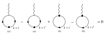
Figura 4: Momentum routing invariance of a tadpole.

We attribute a general loop momentum in the diagrams of Fig. 3, respecting the energy-momentum conservation in the vertices. When the external momentum $p_{\mu}$ is contracted with the diagrams, each one of the graphs, after the contraction is decomposed in a difference of two identical tadpole diagrams with different loop momentum. Considering the six two-point amplitudes, after the contraction with $p_{\mu}$, only four tadpole diagrams survive, which are shown in Fig. 4, in which $l$ is an general routing that is proportional to the external momentum, i.e., $l=\alpha p$. The tadpoles are functions of $l$ ($l^{\prime}$), $\tau^{\nu}(l)$. The result of the calculation represented by Fig. 4 is given by:

$$\tau^{\nu}_{(a)}(l)-\tau^{\nu}_{(a)}(l^{\prime})+\tau^{\nu}_{(b)}(l)-\tau^{\nu}_{(b)}(l^{\prime})=8qc_{\mu\alpha}\left\{(\alpha^{3}-\alpha^{\prime 3})\left[p^{\mu}p^{\alpha}p^{\nu}+p^{2}p^{\alpha}\eta^{\mu\nu}\right](-v_{0}+2\xi_{0}-\sigma_{0})+\right.$$

$$\left.+p^{\alpha}\eta^{\mu\nu}(2\upsilon_{2}-\xi_{2})\right\}+4q(\alpha^{2}-\alpha^{\prime 2})(p^{2}me^{\nu}+2mp^{\nu}e\cdot p)(2\upsilon_{0}-\xi_{0}).$$ (23)

Since $\alpha\neq\alpha^{\prime}$ by definition, the only possible solution for preserving gauge invariance (the tranversality of the photon polarization tensor) is the same that assures momentum routing invariance. In fact, the explicit calculation which results in eq. (23) enforces that $\xi_{0}=2\upsilon_{0}$ and $\sigma_{0}=3\upsilon_{0}$. If we take into account the contributions from the traditional QED, we also obtain that $\upsilon_{2}=\xi_{2}=0$. It is interesting to remark that, although we have considered an arbitrary loop momentum in the vacuum polarization tensor, this result implies momentum routing invariance of the tadpole diagram, which results in transversality of the photon two-point function. In general, the transversality of an amplitude with $n$ external legs will result in routing independence of an amplitude with $n-1$ outer legs. This condition is weaker than the independence of loop-momentum of the original amplitude. Also, MRI looks like a symmetry of the Feynman diagrams, as in Fig. 4. But is not a symmetry in terms of an action, i. e. transformations of the fields that make this action invariant.

The piece $I_{log}(m^{2})$ is a logarithmically divergent integral, namely $\int\frac{d^{4}k}{(2\pi)^{4}}\frac{1}{(k^{2}-m^{2})^{2}}$, introduced in section III. We do not have to evaluate it explicitly. It gives rise to $1/\epsilon+...$ in dimensional regularization, for example. We now take the low energy limit ($m^{2}>>p^{2}$) in each term and integral of eq. (20). For instance, $Z_{1}(m^{2}>>p^{2})\approx-\frac{p^{2}}{12m^{2}}$ in this limit. Thus, we find the low energy limit of the vacuum polarization tensor ($m^{2}>>p^{2}$):

$$\Pi^{\mu\nu}_{LV}(p)=\frac{8}{3}q^{2}\left\{c^{\mu p}p^{\nu}+c^{\nu p}p^{\mu}-c^{pp}\eta^{\mu\nu}-p^{2}c^{\mu\nu}\right\}\left(I_{log}(m^{2})+\frac{i}{16\pi^{2}}\frac{p^{2}}{6m^{2}}+\frac{\upsilon_{0}}{2}\right)+$$

$$+\frac{i}{16\pi^{2}}\frac{q^{2}}{3m^{2}}c^{pp}\left(p^{\mu}p^{\nu}-p^{2}\eta^{\mu\nu}\right)-\frac{mq^{2}}{12\pi^{2}}\frac{p^{2}}{m^{2}}\left\{g^{\mu\nu p}+\frac{1}{p^{2}}(p^{\mu}g^{\nu pp}-p^{\nu}g^{\mu pp})\right\}+$$

$$-4imq^{2}p_{\alpha}\left(g^{\nu\mu\alpha}-g^{\alpha\mu\nu}+g^{\alpha\nu\mu}\right)\upsilon_{0}-\left(\frac{q^{2}}{2\pi^{2}}\right)\epsilon^{bp\mu\nu}\left(1-8i\pi^{2}\upsilon_{0}\right)$$

$$\approx\frac{8}{3}q^{2}\left\{c^{\mu p}p^{\nu}+c^{\nu p}p^{\mu}-c^{pp}\eta^{\mu\nu}-p^{2}c^{\mu\nu}\right\}I_{log}(m^{2})+\frac{i}{16\pi^{2}}\frac{q^{2}}{3m^{2}}c^{pp}\left(p^{\mu}p^{\nu}-p^{2}\eta^{\mu\nu}\right)+$$

$$-\left(\frac{q^{2}}{2\pi^{2}}\right)\epsilon^{bp\mu\nu}\left(1-8i\pi^{2}\upsilon_{0}\right),$$ (24)

where $c^{p\nu}$ stands for $c^{\mu\nu}p_{\mu}$.

The result in eq. (24) shows that only $b_{\mu}$, $c_{\mu\nu}$ and $g_{\mu\nu\lambda}$ affect usual QED at low energies. The one-loop LV contribution to spectroscopy or condensed matter physics would be due only to these terms. In particular, the radiatively induced CFJ term $\epsilon^{\alpha\beta\mu\nu}b_{\alpha}p_{\beta}$ is the one most studied within various contexts and it is dominant compared to terms proportional to $g^{\mu\nu\lambda}$.

On the other hand, in the high-energy limit ($m^{2}<<p^{2}$) we find that vacuum polarization tensor is affected only by $c_{\mu\nu}$ coefficients:

$$\Pi^{\mu\nu}_{LV}(p)=\frac{8}{3}q^{2}\left\{c^{\mu p}p^{\nu}+c^{\nu p}p^{\mu}-c^{pp}\eta^{\mu\nu}-p^{2}c^{\mu\nu}\right\}\left\{I_{log}(m^{2})-\frac{i}{16\pi^{2}}\left[\ln{\left(-\frac{p^{2}}{m^{2}}\right)}-\frac{5}{3}\right]+\frac{\upsilon_{0}}{2}\right\}+$$

$$-\frac{i}{16\pi^{2}}\frac{4}{3}q^{2}c^{pp}\left(\frac{p^{\mu}p^{\nu}}{p^{2}}-\eta^{\mu\nu}\right),$$ (25)

where pieces proportional to $p_{\mu}$ can be disregarded since they couple with currents, and contributions proportional to $\partial_{\mu}J^{\mu}$ vanish due to the gauge symmetry.

V The parameter $b_{\mu}$ and applications to condensed matter

The bridge between high-energy physics and condensed matter has shown promising in recent years and the question of studies on the renormalization group has been the great trump card of this relationship [36]. With the emergence of graphene, low-dimensional systems could be described via the massless Dirac equation in ($2+1$)-dimensional space-time. The application of field theory in low-dimensional systems has become a reality, with regard to theoretical studies, such as the model that describes how electrons propagate over a sheet of graphene, from the point of view of the renormalization group [37]. Another interesting application consists in considering curved space effects in graphene [38], showing how useful is the application of field theory techniques to low-dimensional electronic systems.

The proposal that particles presenting a relativistic scattering relationship can be considered as quasi-particles in condensed matter models has been known for some time [39]. In some models, the dispersion relation can be linearized, by means of an expansion around the Fermi energy, which ends up with relativistic energy-momentum relations. In this sense, Dirac’s fermions gained some prominence with the discovery of graphene which, being an essentially ($2+1$)-dimensional system, is nothing more than a sheet composed of carbon atoms in a hexagonal lattice [40]. Thus, electrons moving over this sheet of carbon interact with the potential of this lattice, giving rise to conical structures close to Fermi energy. Near this region (called a node), the scattering relationships of electrons on the graphene sheet turn out to be linear and the Hamiltonian that describes the system is given by the non-massive Dirac equation, where the propagation velocity is the Fermi velocity ($v_{f}$) and the spin of the particle gives rise to a pseudo-spin, which is related to the sub-lattice of the system.

After the observation of Dirac fermions, it was realized [41] that some materials whose band structure present nodes around the excitation of the material are Weyl fermions, such materials being called Weyl semi-metals [42]. Initially, the Weyl semi-metals proposals were based on studies of pyrochlore iridium molecules, topological insulators and heterostructures [43]. Such descriptions paved the way for the distance between condensed matter and high energy physics to become smaller with regard to the description of certain phenomena, more specifically the emergence of field theory according to Anti-de Sitter-conformal field theory (AdS-CFT) correspondence or Anti-de Sitter-condensed matter theory correspondence (AdS-CMT) [44]. In the case of Weyl semi-metals, this connection occurs through the chiral anomaly, which can be translated into condensed matter models. The chiral anomaly basically tells us that the conservation laws of the vector current ($\partial_{\mu}j^{\mu}=0$) and that of the chiral current ($\partial_{\mu}j^{\mu}_{5}=0$) cannot be satisfied at the same time. Therefore, if we enforce vector current conservation, the chiral current cannot be conserved, which leads to the well-known chiral symmetry breaking. From the point of view of Weyl semi-metals, it can be written in terms of the electromagnetic fields as well as the number of fermions with right-left chirality [45].

Thus, from this perspective, one might wonder whether the inclusion of terms causing the violation of Lorentz symmetry would also lead to interesting results, considering this relationship with condensed matter. In this sense, one can apply QED to a class of materials that can be considered as Weyl semi-metals [46, 47, 48, 49, 50]. With the proper choice of physical parameters, these materials can be represented by the massive Dirac equation in (3 + 1)-dimensions (at low energies, it is considered to describe quasi-particles), which is related to the following action (corresponding to only the $b_{\mu}$ term in equation (1))

$$S=\int d^{4}x\bar{\psi}(i\cancel{\partial}-m-\cancel{b}\gamma_{5}-e\cancel{A})\psi,$$ (26)

with $b_{\mu}$ being a constant four-vector.

This model has been studied with great enthusiasm, since it can generate a CFJ term [13]-[23] that can be finite but undeterminated [11]. However, starting from eq. (26), it is possible to radiatively induce the CFJ term and determine it unambiguously, since condensed matter models can be verified experimentally.

The corresponding action of eq. (26) for the condensed matter model in the momentum space is given by the expression

$$S=\int\frac{d^{4}k}{(2\pi)^{4}}\bar{\psi}(\gamma_{\mu}M^{\mu}_{\nu}k^{\nu}-m-\cancel{b}\gamma_{5})\psi,$$ (27)

with $M^{\mu}_{\nu}=(v_{f},v_{f},\tilde{v}_{f})$ being a diagonal matrix which is necessary due to the anisotropy introduced by the Fermi velocity (in some materials, we consider $v_{f}=c/300$).

The amplitudes and propagators that come from eq. (27) are similar to the usual QED. The complete propagator is given by the expression

$$G(k,b)=\frac{i}{(\cancel{k}-m-\cancel{b}\gamma_{5})},$$ (28)

with the polarization tensor $\Pi^{\mu\nu}$ given by the following expression, already adapted due to the velocity of propagation of the charge carriers on the graphene sheet being the Fermi velocity $v_{f}$,

$$\Pi^{\mu\nu}(b,p)=\frac{e^{2}}{v_{f}\tilde{v}_{f}}\int\frac{d^{4}k}{(2\pi)^{4}}\ Tr[\gamma^{\mu}G(k,b)\gamma^{\nu}G(k+p,b)].$$ (29)

Equation (29) provides all the necessary information regarding the relationship between the Lorentz breaking and the Weyl semi-metals. It is now sufficient to perform a direct calculation to obtain information about the consequences of the parameter $b$. Thus, taking the trace and making the necessary calculations, we found the result for the amplitude given by equation (20), in which only the $b_{\mu}$ parameter contributes to the result for conductivity. From the point of view of implicit regularization, which was discussed in detail in Section III, the parameter $\upsilon_{0}$, even when is required gauge (and/or momentum routing) invariance, is undetermined. In this sense, the process of fixing the parameter should be by phenomenology, like building an experimental apparatus that can measure the 4-current $j_{\mu}$ associated with the fermion current adapted to a condensed matter model (an example of measurement to fix such a parameter is an analysis of the Hall effect from the perspective of Weyl semi-metals, where it is possible to experimentally obtain the value of the so-called Hall conductivity [5]). On the other hand, from a theory point of view, some results agree that the parameter $\upsilon_{0}$ can be determined unambiguously for massless theories [51, 52].

After contracting the $A_{\mu}$ field with the finite piece that remains in eq. (24), we find out the following current

$$j^{\nu}=\frac{q^{2}}{2\pi^{2}v_{f}\tilde{v}_{f}}(1-8\pi^{2}\upsilon_{0})b_{m}\epsilon^{m\nu\alpha\beta}\partial_{\alpha}A_{\beta},$$ (30)

considering the spatial part and

$$j^{\nu}=\frac{q^{2}}{2\pi^{2}v_{f}\tilde{v}_{f}}(1-8\pi^{2}\upsilon_{0})b_{0}\epsilon^{0\nu\alpha\beta}\partial_{\alpha}A_{\beta},$$ (31)

when we consider the temporal part. The spatial part presented by (30) gives rise to the anomalous Hall effect, whose conductivity is proportional to the separation term between the Weyl nodes.

$$\sigma^{xy}=\frac{1}{2\pi^{2}v_{f}\tilde{v}_{f}}\epsilon^{xyl}(1-8\pi^{2}\upsilon_{0})|\vec{b}|\hat{b}_{l}.$$ (32)

The second equation, given by (31), describes the so-called magnetic effect, which sometimes implies the equilibrium of currents in the presence of the chiral magnetic field [53]. However, this is a naive statement, because the chiral anomaly in condensed matter models takes place near the Weyl nodes. Therefore, one must take a great care to predict chiral anomaly effects directly for a Weyl semi-metal (for more details on Weyl semi-metals, see [54]). Nevertheless, we see that Weyl semi-metals are interesting for studies in high energy physics, more specifically, considering that they can be analyzed from the point of view of Lorentz symmetry breaking, when the conductivity can be generated by a $\cancel{b}\gamma_{5}$ type term in the LV action.

A comment here is necessary. The $\Pi^{\mu\nu}$ polarization tensor modifies Maxwell equations. The even part is related to the characteristics of the electrical permeability and magnetic permeability constants of the medium where the electrons propagate. The odd part, on the other hand, can add new terms to Maxwell equations, which can modify the response of the material medium to the propagation of electrons in a Weyl semi-metal. Considering $j=\rho=0$ (absence of sources), the equation of the wave propagating in a Weyl semi-metal is modified, leading to the effect of vacuum birefringence associated with it. This effect is exclusively associated with the CFJ term induced radiatively and such observation is one example of how to fix the parameter $\upsilon_{0}$ by phenomenology. Some other interesting effects on Weyl semi-metals are described in [55] (Repulsive Casimir Effect) and [56] (Axionic Electrodynamics) .

VI Summary

We calculated the polarization tensor of the Abelian gauge field in a minimal LV extension of QED involving all terms listed in [31]. Within our studies, the main attention was paid, first, to divergent contributions, while most of previous studies dealt with finite ones, the most known of them is the CFJ term, second, to the infrared-leading parts of finite contributions. The importance of these terms is justified by the fact that they play a special role within condensed matter studies where the LV effects attract essential attention. In this study, we followed this line and calculated the anomalous Hall conductivity and discussed other possible applications of our results to the condensed matter, especially, to Weyl semi-metals.

A natural continuation of this study, besides of study of other applications of Lorentz symmetry breaking within the condensed matter context, could consist in treating the low-energy impacts of higher-derivative LV terms. We are planning to do this study in a forthcoming paper.

Appendix

All integrals needed after taking the traces in eqs. (4)-(9) can be obtained from integrals below:

$$\int_{k}\frac{1}{[(k-p)^{2}-m^{2}]}=I_{quad}(m^{2})-p^{2}\upsilon_{0};$$ (33)

$$\int_{k}\frac{k^{\alpha}}{[(k-p)^{2}-m^{2}]}=p^{\alpha}(I_{quad}(m^{2})-\upsilon_{2})-p^{2}p^{\alpha}(\xi_{0}-\upsilon_{0});$$ (34)

$$\int_{k}\frac{k^{\alpha}}{[(k-p)^{2}-m^{2}]^{2}}=p^{\alpha}(I_{log}(m^{2})-\upsilon_{0});$$ (35)

$$\int_{k}\frac{k^{2}}{[(k-p)^{2}-m^{2}]^{2}}=I_{quad}(m^{2})+(m^{2}+p^{2})I_{log}(m^{2})-3p^{2}\upsilon_{0};$$ (36)

$$\int_{k}\frac{k^{\alpha}k^{\beta}}{[(k-p)^{2}-m^{2}]^{2}}=\frac{1}{2}g^{\alpha\beta}(I_{quad}(m^{2})-\upsilon_{2})+p^{\alpha}p^{\beta}(I_{log}(m^{2})-\xi_{0})-\frac{1}{2}p^{2}g^{\alpha\beta}(\xi_{0}-\upsilon_{0});$$ (37)

$$\int_{k}\frac{k^{2}k^{\alpha}}{[(k-p)^{2}-m^{2}]^{2}}=2p^{\alpha}(I_{quad}(m^{2})-\upsilon_{2})+p^{\alpha}(m^{2}+p^{2})I_{log}(m^{2})+p^{\alpha}(3p^{2}-m^{2})\upsilon_{0}-4p^{2}p^{\alpha}\xi_{0};$$ (38)

$$\int_{k}\frac{k^{\alpha}k^{\beta}k^{\gamma}}{[(k-p)^{2}-m^{2}]^{2}}=\frac{1}{2}p^{\{\alpha}g^{\gamma\beta\}}\left[I_{quad}(m^{2})-\xi_{2}\right]-\frac{1}{2}p^{2}p^{\{\alpha}g^{\gamma\beta\}}\left[I_{log}(m^{2})-\xi_{0}\right]+$$

$$\;\;\;\;\;\;\;\;\;\;\;\;\;\;\;\;\;\;\;\;\;\;\;\;\;\;\;\;\;\;\;\;+\frac{1}{2}(p^{2}p^{\{\alpha}g^{\gamma\beta\}}+2p^{\alpha}p^{\beta}p^{\gamma})\left[I_{log}(m^{2})-\sigma_{0}\right];$$ (39)

$$I=\int_{k}\frac{1}{(k^{2}-m^{2})^{2}[(k+p)^{2}-m^{2}]}=-b\ \int^{1}_{0}dx\frac{(1-x)}{\Delta^{2}};$$ (40)

$$I_{1}^{\beta}=\int_{k}\frac{k^{\beta}}{(k^{2}-m^{2})^{2}[(k+p)^{2}-m^{2}]}=b\ p^{\beta}\ \int^{1}_{0}dx\frac{x(1-x)}{\Delta^{2}};$$ (41)

$$J_{1}^{\beta}=\int_{k}\frac{k^{\beta}}{(k^{2}-m^{2})[(k-p)^{2}-m^{2}]^{2}}=I_{1}^{\beta}+p^{\beta}I;$$ (42)

$$I_{2}=\int_{k}\frac{k^{2}}{(k^{2}-m^{2})^{2}[(k+p)^{2}-m^{2}]}=I_{log}(m^{2})-b\ Z_{0}(p^{2},m^{2})-b\ m^{2}\ \int^{1}_{0}dx\frac{(1-x)}{\Delta^{2}}$$ (43)

$$J_{2}=\int_{k}\frac{k^{2}}{(k^{2}-m^{2})[(k-p)^{2}-m^{2}]^{2}}=I_{2}+p^{2}I+2p_{\beta}I_{1}^{\beta};$$ (44)

$$I_{2}^{\beta\nu}=\int_{k}\frac{k^{\beta}k^{\nu}}{(k^{2}-m^{2})^{2}[(k+p)^{2}-m^{2}]}=\frac{1}{4}g^{\beta\nu}(I_{log}(m^{2})-\upsilon_{0})-\frac{1}{2}b\ g^{\beta\nu}[Z_{0}(p^{2},m^{2})-Z_{1}(p^{2},m^{2})]-$$

$$-b\ p^{\beta}p^{\nu}\ \int^{1}_{0}dx\frac{x^{2}(1-x)}{\Delta^{2}};$$ (45)

$$J_{2}^{\beta\nu}=\int_{k}\frac{k^{\beta}k^{\nu}}{(k^{2}-m^{2})[(k-p)^{2}-m^{2}]^{2}}=I_{2}^{\beta\nu}+p^{\beta}p^{\nu}I+I_{1}^{\beta}p^{\nu}+I_{1}^{\nu}p^{\beta};$$ (46)

$$I_{3}^{\nu}=\int_{k}\frac{k^{2}k^{\nu}}{(k^{2}-m^{2})^{2}[(k+p)^{2}-m^{2}]}=-\frac{1}{2}p^{\nu}(I_{log}(m^{2})-\upsilon_{0})+b\ p^{\nu}Z_{1}(p^{2},m^{2})+b\ m^{2}\ p^{\nu}\int^{1}_{0}dx\frac{x(1-x)}{\Delta^{2}};$$ (47)

$$J_{3}^{\nu}=\int_{k}\frac{k^{2}k^{\nu}}{(k^{2}-m^{2})[(k-p)^{2}-m^{2}]^{2}}=I_{3}^{\nu}+p^{\nu}I_{2}+p^{2}I_{1}^{\nu}+p^{2}p^{\nu}I+2p_{\gamma}I_{2}^{\gamma\nu}+2p_{\gamma}p^{\nu}I_{1}^{\gamma}-p^{\nu}\upsilon_{0};$$ (48)

$$I_{5}^{\beta\nu\alpha}=\int_{k}\frac{k^{\beta}k^{\nu}k^{\alpha}}{(k^{2}-m^{2})^{2}[(k+p)^{2}-m^{2}]}=\frac{-1}{12}bp^{\{\alpha}g^{\beta\nu\}}(I_{log}(m^{2})-\xi_{0})+b\ p^{\alpha}p^{\beta}p^{\nu}\int^{1}_{0}dx\frac{x^{3}(1-x)}{\Delta^{2}}+$$

$$+\frac{1}{2}b\ p^{\{\alpha}g^{\beta\nu\}}[Z_{1}(p^{2},m^{2})-Z_{2}(p^{2},m^{2})];$$ (49)

$$J_{5}^{\beta\nu\alpha}=\int_{k}\frac{k^{\beta}k^{\nu}k^{\alpha}}{(k^{2}-m^{2})[(k-p)^{2}-m^{2}]^{2}}=I_{5}^{\beta\nu\alpha}+p^{\beta}p^{\nu}p^{\alpha}I+p^{\{\nu}p^{\beta}I^{\alpha\}}_{1}+p^{\{\beta}I^{\nu\alpha\}}_{2}+\frac{1}{4}p^{\{\alpha}g^{\beta\nu\}}(\upsilon_{0}-\xi_{0})$$ (50)

$$I_{4}^{\beta\nu}=\int_{k}\frac{k^{2}k^{\beta}k^{\nu}}{(k^{2}-m^{2})^{2}[(k+p)^{2}-m^{2}]}=\frac{1}{2}g^{\beta\nu}(I_{quad}(m^{2})-\upsilon_{2})+\frac{1}{4}(m^{2}-p^{2})g^{\beta\nu}(I_{log}(m^{2})-\upsilon_{0})+$$

$$+\frac{1}{6}(p^{2}g^{\nu\beta}+2p^{\beta}p^{\nu})(I_{log}(m^{2})-\xi_{0})-b\ (-g^{\beta\nu}p^{2}+p^{\nu}p^{\beta})Z_{2}(p^{2},m^{2})+\frac{1}{2}\ b(m^{2}-3p^{2})\ g^{\beta\nu}Z_{1}(p^{2},m^{2})+$$

$$+\frac{1}{2}b(p^{2}-m^{2})g^{\beta\nu}Z_{0}(p^{2},m^{2})-b\ p^{\beta}p^{\nu}m^{2}\ \int^{1}_{0}dx\frac{x^{2}(1-x)}{\Delta^{2}};$$ (51)

$$J_{4}^{\beta\nu}=\int_{k}\frac{k^{2}k^{\beta}k^{\nu}}{(k^{2}-m^{2})[(k-p)^{2}-m^{2}]^{2}}=\frac{1}{2}g^{\nu\beta}(I_{quad}(m^{2})-\upsilon_{2})+(m^{2}-p^{2})J_{2}^{\beta\nu}+2p_{\lambda}J_{5}^{\beta\nu\lambda}-2p_{\lambda}I_{5}^{\beta\nu\lambda}-p^{2}I_{2}^{\beta\nu},$$ (52)

where $b\equiv\frac{i}{(4\pi)^{2}}$, $Z_{k}(p^{2},m^{2})$ and $\Delta^{2}$ are defined as

$$Z_{k}(p^{2},m^{2})=\int^{1}_{0}dzz^{k}\ln\frac{m^{2}-p^{2}z(1-z)}{m^{2}},$$ (53)

$$\Delta^{2}=m^{2}-p^{2}x(1-x).$$ (54)

The basic divergent integrals $I_{log}(m^{2})$ and $I_{quad}(m^{2})$ and the surface terms $\upsilon_{0}$, $\upsilon_{2}$ and $\xi_{0}$ are defined in section III.

• [1] D. Colladay and V. A. Kostelecký, Phys. Rev. D 58, 116002 (1998).
• [2] V. Alan Kostelecky and S. Samuel, Phys.Rev. D, 39, 683 (1989).
• [3] S. M. Carroll, J. A. Harvey, V. Alan Kostelecký, C. D. Lane and T. Okamoto, Phys.Rev. Lett., 87, 141601 (2001).
• [4] W. F. Chen and G. Kunstatter, Phys. Rev. D, 62, 105019 (2000).
• [5] A. G. Grushin, Phys. Rev. D, 86, 045001 (2012).
• [6] P. D. S. Silva, L. Lisboa-Santos, M. M. Ferreira, Jr. and M. Schreck, Phys. Rev. D 104, 116023 (2021).
• [7] V. A. Kostelecký, C. D. Lane and A. G. Pickering, Phys. Rev. D 65, 056006 (2002).
• [8] D. Colladay and P. McDonald, Phys. Rev. D, 79, 125019 (2009).
• [9] D. Colladay and P. McDonald, Phys. Rev. D 75, 105002 (2007).
• [10] D. Colladay and P. McDonald, Phys. Rev. D 77, 085006 (2008).
• [11] R. Jackiw, Int. J. Mod. Phys. B, 14, 2011 (2000).
• [12] V. A. Kostelecky, R. Lehnert, N. McGinnis, M. Schreck and B. Seradjeh, Phys. Rev. Res. 4, 023106 (2022).
• [13] R. Jackiw and V. A. Kostelecký, Phys. Rev. Lett. 82, 3572 (1999);
• [14] J. M. Chung and Phillial Oh, Phys. Rev. D 60, 067702 (1999).
• [15] M. Perez-Victoria, Phys. Rev. Lett. 83, 2518 (1999).
• [16] B. Altschul, Phys. Rev. D 69, 125009 (2004).
• [17] B. Altschul, Phys. Rev. D 70, 101701 (2004).
• [18] J. R. Nascimento, E. Passos, A. Yu. Petrov and F. A. Brito, J. High Energy Phys. 06 (2007) 016.
• [19] J. Alfaro, A. A. Andrianov, M. Cambiaso, P. Giacconi and R. Soldati, Int. J. Mod. Phys. A 25, 3271 (2010).
• [20] A. P. B. Scarpelli, M. Sampaio, M. C. Nemes and B. Hiller, Eur. Phys. J. C 56, 571 (2008).
• [21] G. Gazzola, H. G. Fargnoli, A. P. B. Scarpelli, M. Sampaio, M. C. Nemes, J. Phys. G 39, 035002 (2012).
• [22] J. C. C. Felipe, A. R. Vieira, A. L. Cherchiglia, A. P. B. Scarpelli and M. Sampaio, Phys. Rev. D 89, 105034 (2014).
• [23] B. Altschul, Phys. Rev. D 99, 125009, (2019).
• [24] G. ’t Hooft and M. Veltman, Nucl. Phys. B, 44, 189-213 (1972).
• [25] C. G. Bollini and J. J. Giambiagi, Nuovo Cim. B, 12, 20 (1972).
• [26] F. Jegerlehner, Eur. Phys. J. C, 18, 673 (2001).
• [27] G. Cynolter and E. Lendvai, Mod. Phys. Lett. A, 26, 1537 (2011).
• [28] Er-Cheng Tsai, Phys. Rev. D, 83, 025020 (2011); Er-Cheng Tsai, Phys. Rev. D, 83, 065011 (2011).
• [29] O. A. Battistel, A. L. Mota and M. C. Nemes, Mod. Phys. Lett. A, 13, 1597 (1998).
• [30] A. C. D. Viglioni, A. L. Cherchiglia, A. R. Vieira, Brigitte Hiller and Marcos Sampaio, Phys. Rev. D, 94, 065023 (2016).
• [31] V. A. Kostelecky, C. D. Lane and A. G. M. Pickering, Phys. Rev. D 65 (2002), 056006.
• [32] B. Altschul, J. Phys. A 39, 13757 (2006).
• [33] D. C. Arias-Perdomo, A. L. Cherchiglia, B. Hiller and M. Sampaio, Symmetry 13, 956 (2021).
• [34] B. Z. Felippe, A. P. B. Scarpelli, A. R. Vieira, J. C. C. Felipe, Eur. Phys. J. C 82, 583 (2022).
• [35] S. M. Carroll, G. B. Field, and R. Jackiw, Phys. Rev. D 41, 1231 (1990).
• [36] D. J. Amit and V. Martin-Mayor, Field Theory, The Renormalization Group and Critical Phenomena (World Scientific, Singapore, (2005).
• [37] J. Gonzalez, F. Guinea, and M. Vozmediano, Nucl. Phys. B 424, 595 (1994).
• [38] F. de Juan, A. Cortijo, and M. A. Vozmediano, Nucl. Phys. B 828, 625 (2010).
• [39] A. O. Gongolin, A. E. Nersesyan and A. M. Tsvelik, Cambridge University Press (1998).
• [40] A. H. C. Neto, Rev. Mod. Phys. 81, 109 (2009).
• [41] G. Xu, Phys. Rev. Lett. 107, 186806 (2011).
• [42] A. M. Turner and A. Vishwanath, arXiv: 1301.0330.
• [43] A. A. Burkov and L. Balents, Phys. Rev. Lett. 107, 127205 (2011).
• [44] A. Sachdev, Sci. Am. Phys. 308, 44 (2013).
• [45] H. B. Nielsen and M. Ninomiya, Phys. Lett. B105, 219 (1981).
• [46] L. Balents, Physics 4, 36 (2011).
• [47] X. Wan, A. M. Turner, A. Vishwanath, and S. Y. Savrasov, Phys. Rev. B 83, 205101 (2011).
• [48] A. A. Burkov and L. Balents, Phys. Rev. Lett. 107, 127205 (2011).
• [49] A. A. Burkov, M. D. Hook, and L. Balents, Phys. Rev. B 84, 235126 (2011).
• [50] S. Rao, Weyl semi-metals: a short review, arXiv: 1603.02821.
• [51] M. Perez-Victoria, Phys. Rev. Lett. 83, 2518 (1999)
• [52] F. A. Brito, L. S. Grigorio, M. S. Guimaraes, E. Passos, and C. Wotzasek, Phys. Rev. D 78, 125023 (2008).
• [53] J. Zhou, Chin. Phys. Lett. 30, 027101 (2013).
• [54] Haldane et al, WPI-MANA, online at http://wwwphy.princeton.edu/aldane/research.html. (2014).
• [55] A. G. Grushin and A. Cortijo, Phys. Rev. Lett. 106, 020403 (2011).
• [56] X.-L. Qi, R. Li, J. Zang, and S.-C. Zhang, Science 323, 1184 (2009).