Neural Capacitated Clustering

Abstract

Recent work on deep clustering has found new promising methods also for constrained clustering problems. Their typically pairwise constraints often can be used to guide the partitioning of the data. Many problems however, feature cluster-level constraints, e.g. the Capacitated Clustering Problem (CCP), where each point has a weight and the total weight sum of all points in each cluster is bounded by a prescribed capacity. In this paper we propose a new method for the CCP, Neural Capacited Clustering, that learns a neural network to predict the assignment probabilities of points to cluster centers from a data set of optimal or near optimal past solutions of other problem instances. During inference, the resulting scores are then used in an iterative k-means like procedure to refine the assignment under capacity constraints. In our experiments on artificial data and two real world datasets our approach outperforms several state-of-the-art mathematical and heuristic solvers from the literature. Moreover, we apply our method in the context of a cluster-first-route-second approach to the Capacitated Vehicle Routing Problem (CVRP) and show competitive results on the well-known Uchoa benchmark.

1 Introduction

In recent years much progress has been achieved in applying deep learning methods to solve classical clustering problems. Due to its ability to leverage prior knowledge and information to guide the partitioning of the data, constrained clustering in particular has recently gained increasing traction. It is often used to incorporate existing domain knowledge in the form of pairwise constraints expressed in terms of must-link and cannot-link relations Wagstaff et al. (2001). However, another type of constraints has been largely ignored so far: cluster level constraints. This type of constraint can for example restrict each assignment group in terms of the total sum of weights which are associated with its members. The simplest case of such a constraint is the maximum size of the cluster, where each point exhibits a weight of one. In the more general case, weights and cluster capacities are real valued and can model a plenitude of practical applications.

Machine learning approaches are particularly well suited for cases in which many similar problems, i.e. problems from the same distribution, have to be solved. In general, most capacitated mobile facility location problems (CMFLP) Raghavan et al. (2019) represent this setting when treating every relocation as a new problem. This is e.g. the case when considering to plan the location of disaster relief services or mobile vaccination centers for several days, where the relocation cost can be considered to be zero since the team has to return to restock at the end of the day. Other applications are for example the planning of the layout of factory floors which change for different projects or logistics problems like staff collection and dispatching Negreiros et al. (2022). Thus, we can utilize supervised learning to learn from existing data how to solve new unseen instances.

The corresponding formulation gives rise to well-known problems from combinatorial optimization, the capacitated $p$-median problem (CPMP) Ross and Soland (1977) where each center has to be an existing point of the data and the capacitated centered clustering problem (CCCP) Negreiros and Palhano (2006) where cluster centers correspond to the geometric center of their members. The general objective is to select a number $K$ of cluster centers and find an assignment of points such that the total distance between the points and their corresponding centers is minimized while respecting the cluster capacity. Both problems are known to be NP-hard and have been extensively studied Negreiros and Palhano (2006).

1.0.1 Contributions

• We propose the first approach to solve general Capacitated Clustering Problems based on deep learning.

• Our problem formulation includes well-known problem variants like the CPMP and CCCP as well as more simple constraints on the cluster size.

• The presented approach achieves competitive performance on several artificial and real world datasets, compared to methods based on mathematical solvers while reducing run time by up to one order of magnitude.

• We present a cluster-first-route-second extension of our method as effective construction heuristic for the CVRP.

2 Background

A typical clustering task is concerned with the grouping of elements in the given data and is normally done in an unsupervised fashion. This grouping can be achieved in different ways where we usually distinguish between partitioning and hierarchical approaches Jain et al. (1999). In this work we are mainly concerned with partitioning methods, i.e. methods that partition the data into different disjoint sub-sets without any hierarchical structure. Although clustering methods can be applied to many varying data modalities like user profiles or documents, in this work we consider the specific case of spatial clustering Grubesic et al. (2014), that normally assumes points to be located in a metric space of dimension $D$, a setting often encountered in practical applications like the facility location problem Ross and Soland (1977).

2.1 Capacitated Clustering Problems (CCPs)

Let there be a set of $n$ points $N=\{1,2,\dots,n\}$ with corresponding feature vectors $x_{i}\in\operatorname{\mathbb{R}}^{D}$ of coordinates and a respective weight $q_{i}\in\mathbb{R}$ associated with each point $i\in N$. Further, we assume that we can compute a distance measure $d(x_{i},x_{j})$ for all pairs of points $i,j\in N$. Then we are concerned with finding a set of $K$ capacitated disjoint clusters $c_{k}\in C,\ c_{k}\subset N,\ c_{k}\cap c_{l}=\emptyset\ \forall k,l\in\{1,\dots,K\}$ with capacities $Q_{k}>0$. The assignment of points to these clusters is given by the set of binary decision variables $y_{ik}$, which are 1 if point $i$ is a member of cluster $k$ and 0 otherwise.

2.1.1 Capacitated $p$-Median Problem

For the CPMP the set of possible cluster medoids is given by the set of all data points $N$ and the objective is to minimize the distance (or dissimilarity) $d(x_{i},x_{m_{k}})$ between all $i$ and their cluster medoid $m_{k}$:

$$\min\sum_{i\in N}\sum_{k\in K}d(x_{i},x_{m_{k}})y_{ik}$$ (1)

s.t.

$$\sum_{k\in K}y_{ik} =1,\quad\forall i\in N,\quad\forall k\in K,$$ (2)

$$\sum_{i\in N}q_{i}y_{ik} \leq Q_{k},\quad\forall k\in K,$$ (3)

$$m_{k} =\operatorname*{argmin}_{m\in c_{k}}\sum_{i\in c_{k}}d(x_{i},x_{m}),$$ (4)

$$y_{ik} \in\{0,1\},\quad\forall i\in N,\quad\forall k\in K,$$ (5)

where each point is assigned to only one cluster (2), all clusters respect the capacity constraint (3), medoids are selected minimizing the dissimilarity of cluster $c_{k}$ (4) and $y$ being a binary decision variable (5).

2.1.2 Capacitated Centered Clustering Problem

In the CCCP formulation, instead of medoids selected among the data points, centroids $\mu_{k}$ are considered, which correspond to the geometric center of the points assigned to each cluster $c_{k}$, replacing (4) with

$$\mu_{k}=\operatorname*{argmin}_{\mu\in\operatorname{\mathbb{R}}^{D}}\sum_{i\in c_{k}}d(x_{i},\mu),$$ (6)

which in the case of the Euclidean space for spatial clustering considered in this paper has a closed form formulation:

$$\mu_{k}=\frac{1}{|c_{k}|}\sum_{i\in N}x_{i}y_{ik},$$ (7)

with $|c_{k}|$ as cardinality of cluster $c_{k}$. This leads to the new minimization objective of

$$\min\sum_{i\in N}\sum_{k\in K}d(x_{i},\mu_{k})y_{ik}.$$ (8)

3 Related Work

Clustering Algorithms

Traditional partitioning methods to solve clustering problems, like the well-known k-means algorithm MacQueen (1967) have been researched for more than half a century. Meanwhile, there exists a plethora of different methods including Gaussian Mixture Models McLachlan and Basford (1988), density based models like DBSCAN Ester et al. (1996) and graph theoretic approaches Ozawa (1985). Many of these algorithms have been extended to solve other problem variants like the CCP. In particular Mulvey and Beck (1984) introduce a k-medoids algorithm utilizing a regret heuristic for the assignment step combined with additional re-locations during an integrated local search procedure while Geetha et al. (2009) propose an adapted version of k-means which instead uses a priority heuristic to assign points to capacitated clusters.

Meta-Heuristics

Apart from direct clustering approaches there are also methods from the operations research community which tackle CCPs or similar formulations like the facility location problem. Different algorithms were proposed modeling and solving the CCP as General Assignment Problem (GAP) Ross and Soland (1977), via simulated annealing and tabu search Osman and Christofides (1994), with genetic algorithms Lorena and Furtado (2001) or using a scatter search heuristic Scheuerer and Wendolsky (2006).

Math-Heuristics

In contrast to meta-heuristics, math-heuristics combine heuristic methods with powerful mathematical programming solvers like Gurobi Gurobi Optimization, LLC (2023), which are able to solve small scale instance to optimality and have shown superior performance to traditional meta-heuristics in recent studies. Stefanello et al. (2015) combine the mathematical solution of the CPMP with a heuristic post-optimization routine in case no optimality was achieved. The math-heuristic proposed in Gnägi and Baumann (2021) comprises two phases: First, a global optimization phase is executed. This phase alternates between an assignment step, which solves a special case of the GAP as a binary linear program (BLP) for fixed medoids, and a median update step, selecting new medoids $m_{k}$ minimizing the total distance to all cluster members under the current assignment. This is followed by a local optimization phase relocating points by solving a second BLP for the sub-set of clusters which comprises the largest unused capacity. Finally, the PACK algorithm introduced in Lähderanta et al. (2021) employs a block coordinate descent similar to the method of Gnägi and Baumann (2021) where the assignment step is solved with Gurobi and the step updating the centers is computed following eq. 7 according to the current assignment.

Deep Clustering

Since the dawn of deep learning, an increasing number of approaches in related fields is employing deep neural networks. Most approaches in the clustering area are mainly concerned with learning better representations for downstream clustering algorithms, e.g. by employing auto-encoders to different data modalities Tian et al. (2014); Xie et al. (2016); Guo et al. (2017); Yang et al. (2017), often trained with enhanced objective functions, which, apart from the representation loss, also include a component approximating the clustering objective and additional regularization to prevent the embedding space from collapsing. A comprehensive survey on the latest methods is given in Ren et al. (2022). More recently, deep approaches for constrained clustering have been proposed: Genevay et al. (2019) reformulate the clustering problem in terms of optimal transport to enforce constraints on the size of the clusters. Zhang et al. (2021) present a framework describing different loss components to include pairwise, triplet, cardinality and instance level constraints into auto-encoder based deep embedded clustering approaches. Finally, Manduchi et al. (2021) propose a new deep conditional Gaussian Mixture Model (GMM), which can include pairwise and instance level constraints. Usually, the described deep approaches are evaluated on very large, high dimensional datasets like MNIST LeCun and Cortes (2010) or Reuters Xie et al. (2016), on which classical algorithms are not competitive. This is in strong contrast to spatial clustering with additional capacity constraints, for which we propose the first deep learning based method.

4 Proposed Method

4.1 Capacitated k-means

The capacitated k-means method proposed by Geetha et al. (2009) changes the assignment step in Lloyd’s algorithm Lloyd (1982), which is usually used to compute k-means clustering. To adapt the procedure to the CCP, the authors first select the $K$ points with the highest weights $q$ as initial centers, instead of selecting them randomly. Moreover, they introduce priorities $\omega_{ik}$ for each point $i$ by dividing its weight $q_{i}$ by its distance to the center of cluster $k$:

$$\omega_{ik}=\frac{q_{i}}{d(x_{i},\mu_{k})}.$$ (9)

Then the list of priorities is sorted and nodes are sequentially assigned to the centers according to their priority. The idea is to first assign points with large weights to close centers and only then points with smaller weight, which can be more easily assigned to other clusters. Next, the centroids are recomputed via the arithmetic mean of the group members (eq. 7). The corresponding pseudo code is given in Alg. 1.

input :  $K$, $n$, coordinates $x$, weights $q$, cluster capacity $Q$, convergence condition $\delta$

output : binary assignment matrix Y

1 $M\leftarrow$ $\text{init}_{\text{topk\_weights}}$ ($x,q,K$)

2 while not  $\delta(x,M,Y)$ do

       $\text{Y}\leftarrow$ allzero ($n,K$)

        // reset assignment

       $\text{Q}\leftarrow$ repeat ($Q,K$)

        // reset capacities

3       foreach $i\in N$ do

4             compute priorities for all clusters (eq. 9)

5      sort priorities, insert into queue $S$

6       while $S$ not empty do

7             get next $i,k$ from $S$

8             if $i$ unassigned and $\text{Q}_{k}\geq q_{i}$ then

                   $\text{Y}_{ik}\leftarrow 1$

                    // cluster assignment

                   $\text{Q}_{k}\leftarrow\text{Q}_{k}-q_{i}$

                    // update capacity

9                  

10      foreach $k\in\{1,\dots,K\}$ do

11             update centroids via eq. 7

return Y

Algorithm 1 Capacitated k-means

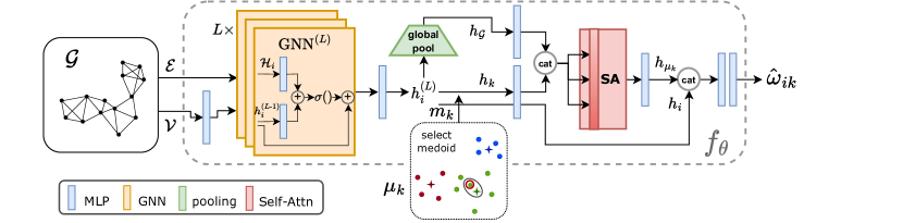
Figure 1: Visualization of the neural scoring function architecture.

While this heuristic works, it can easily lead to sub-optimal allocations and situations in which no feasible solution can be found, e.g. in cases where many nodes with high weight are located very far from the cluster centers. To solve these problems we propose several modifications to the algorithm.

4.2 Neural Scoring Functions

The first proposed adaption is to learn a neural scoring function $f_{\theta}$ with parameters $\theta$, which predicts the probability of each node $i$ to belong to cluster $k$:

$$\hat{\omega}_{ik}=f_{\theta}(\operatorname{\mathcal{G}},\mu_{k})$$ (10)

For that purpose we first create a graph representation $\operatorname{\mathcal{G}}=(\mathcal{V},\mathcal{E})$ of the points by connecting each point with its $\mathcal{K}$ nearest neighbors, producing edges $e_{ij}\in\mathcal{E}$ with edge weights $d(x_{i},x_{j})$. Nodes $v_{i}\in\mathcal{V}$ are created by concatenating the respective coordinates and weights $[x_{i};q_{i}]$. This graph allows us to define a structure on which the relative spatial information of the different points can be efficiently propagated. We encode $\operatorname{\mathcal{G}}$ with the Graph Neural Network (GNN) introduced in Morris et al. (2019), which is able to directly work with edge weights by employing the graph operator defined as

where $h^{(l-1)}_{i}\in\operatorname{\mathbb{R}}^{1\times d_{\text{emb}}}$ represents the embedding of node $i$ at the previous layer $l-1$, $\mathcal{H}(i)$ is the 1-hop graph neighborhood of node $i$, $e_{ji}$ is the directed edge connecting nodes $j$ and $i$, $\operatorname{MLP}_{1}$ and $\operatorname{MLP}_{2}$ are Multi-Layer Perceptrons $\operatorname{MLP}:\operatorname{\mathbb{R}}^{d_{\text{emb}}}\to\operatorname{\mathbb{R}}^{d_{\text{emb}}}$ and $\sigma()$ is a suitable activation function. Furthermore, we add residual connections and regularization to each layer. In our case we choose GELU Hendrycks and Gimpel (2016) and layer normalization Ba et al. (2016) which outperformed ReLU and BatchNorm in preliminary experiments. The input layer projects the node features $v_{i}=[x_{i};q_{i}]\in\operatorname{\mathbb{R}}^{D+1}$ to the embedding dimension $d_{\text{emb}}$ using a feed forward layer, which then is followed by $L$ GNN layers of the form given in eq. 11. In order to create embeddings $h_{\mu_{k}}$ for the centers $\mu_{k}\in M$ we find the node $j$ closest to $\mu_{k}$ (corresponding to the cluster medoid $m_{k}$) and select its embedding $h^{(L)}_{j}$ as $h_{k}$. This embedding is concatenated with a globally pooled graph embedding $h_{\operatorname{\mathcal{G}}}\in\operatorname{\mathbb{R}}^{d_{\text{emb}}}$:

$$h_{\operatorname{\mathcal{G}}}=\operatorname{MLP}_{\operatorname{\mathcal{G}}}\left(\big{[}\operatorname{MAX}(h^{(L)});\operatorname{MEAN}(h^{(L)})\big{]}\right)$$ (12)

with $\operatorname{MLP}_{\operatorname{\mathcal{G}}}:\operatorname{\mathbb{R}}^{2d_{\text{emb}}}\to\operatorname{\mathbb{R}}^{d_{\text{emb}}}$. Next, in order to model the interdependence of different centers, their resulting vectors are fed into a self attention layer (SA) Vaswani et al. (2017) followed by another $\operatorname{MLP}_{\mu}:\operatorname{\mathbb{R}}^{2d_{\text{emb}}}\to\operatorname{\mathbb{R}}^{d_{\text{emb}}}$:

$$h_{\mu_{k}}=\operatorname{MLP}_{\mu}\big{(}\operatorname{SA}\left(\left[h_{\operatorname{\mathcal{G}}};h_{k}\right]\right)\big{)}.$$ (13)

Since we feed a batch of all points $N$ and all currently available centers $\mu$ to our model, they are encoded as a batch of context vectors $h_{\mu_{k}}$, one for each cluster $k\in\{1,\dots,K\}$. The SA module then models the importance of all cluster center configurations $h_{\mu}$ for each cluster $k$ which allows the model to effectively decide about the cluster assignment probability of every node $i$ to each cluster $c_{k}$ conditionally on the full information encoded in the latent context embeddings $h_{\mu}$. Finally, we do conditional decoding by concatenating every center embedding with each node and applying a final stack of (element-wise) MLPs. The architecture of our neural scoring function is shown in Figure 1.

Training the model

We create the required training data and labels by running the math-heuristic solver of Gnägi and Baumann (2021) on some generated datasets to create a good (although not necessarily optimal) partitioning. Then we do supervised training using binary cross entropy (BCE) with pairwise prediction of the assignment of nodes $i$ to clusters $k$.

4.3 Neural Capacitated Clustering

To fully leverage our score estimator we propose several adaptions and improvements to the original capacitated k-means algorithm (Alg. 1). The new method, which we dub Neural Capacitated Clustering (NCC) is described in Alg. 2.

4.3.1 Order of assignment

Instead of sorting all center-node pairs by their priority and then sequentially assigning them according to that list, we fix an order given by permutation $\pi$ for the centers and cycle through each of them, assigning one node at a time. Since the output of $f_{\theta}$ is the log probability of point $i$ belonging to cluster $k$ and its magnitude does not directly inform the order of assignments of different nodes $i$ and $j$ in the iterative cluster procedure, we found it helpful to scale the output of $f_{\theta}$ by the heuristic weights introduced in eq. 9. Thus, we assign that node $i$ to cluster $k$, which has the highest scaled conditional priority and still can be accommodated considering the remaining capacity $Q_{k}$. In case there remain any unassigned points $j$ at the end of an iteration, which cannot be assigned to any cluster since $q_{j}>Q_{k}\ \forall k\in K$, we assign them to a dummy cluster $K+1$ located at the origin of the coordinate system. We observe in our experiments that already after a small number of iterations usually no nodes are assigned to the dummy cluster anymore, meaning a feasible allocation has been established. Moreover, since the neighborhood graph $\operatorname{\mathcal{G}}$ does not change between iterations, we can speed up the calculation of priorities by pre-computing and buffering the node embeddings $h_{i}$ and graph embedding $h_{\operatorname{\mathcal{G}}}$ in the first iteration.

4.3.2 Re-prioritization of last assignments

This is motivated by the observation that the last few assignments are the most difficult, since they have to cope with highly constrained center capacities. Thus, relying on the predefined cyclic order of the centers (which until this point has ensured that approx. the same number of nodes was assigned to each cluster) can lead to sub-optimal assignments in case some clusters have many nodes with very large or very small weights. To circumvent this problem we propose two different assignment strategies:

1. Greedy:  We treat the maximum (unscaled) priority over all clusters as an absolute priority $\bar{\omega}_{i}$ for all remaining unassigned points $i$:

   $$\bar{\omega}_{i}=\max_{k}\ \hat{\omega}_{ik}$$ (14)

   Then the points are ordered by that priority and sequentially assigned to the closest cluster which can still accommodate them.

2. Sampling:  We normalize the absolute priorities $\bar{\omega}_{i}$ of all remaining unassigned points $i$ via the softmax function and treat them as probabilities according to which they are sequentially sampled and assigned to the closest cluster which can still accommodate them. This procedure can be further improved by sampling several assignment rollouts and selecting the configuration, which leads to the smallest resulting inertia.

The fraction $\alpha$ of final nodes for which the re-prioritization is applied we treat as a hyperparameter.

4.3.3 Weight-adapted kmeans++ initialization

As found in the study of Celebi et al. (2013) standard methods for the selection of seed points for centers during the initialization of k-means algorithms perform quite poorly. This is why the k-means++ Arthur and Vassilvitskii (2006) initialization routine was developed, which aims to maximally spread out the cluster centers over the data domain, by sampling a first center uniformly from the data and then sequentially sampling the next center from the remaining data points with a probability equal to the normalized squared distance to the closest already existing center. We propose a small modification to the k-means++ procedure (called ckm++), that includes the weight information into the sampling procedure by simply multiplying the squared distance to the closest existing cluster center by the weight of the data point to sample.

input :  $K$, $n$, coordinates $x$, weights $q$, cluster capacity $Q$, convergence condition $\delta$, scoring function $f_{\theta}$, fraction $\alpha$

output : binary assignment matrix Y

$M\leftarrow$ $\text{init}_{\text{ckm++}}$ ($x,q,K$)

  // get seed centers

$\operatorname{\mathcal{G}}\leftarrow$ KNN_graph (x)

  // create graph

1 while not  $\delta(x,M,Y)$ do

2       $\text{Y}\leftarrow$ allzero ($n,K\text{+}1$)

3       $\text{Q}\leftarrow$ repeat ($Q,K$)

4       $\pi\leftarrow$ random_perm ($\{1,\dots,K\}$)

       $\hat{\omega}\leftarrow f_{\theta}(\operatorname{\mathcal{G}},M)$

        // compute priorities

5       sort columns of $\hat{\omega}$

6       while any $i$ can be assigned do

7             $k\leftarrow\pi$.get_next ()

8             foreach $i\in N$ sorted by $\hat{\omega}_{k}$ do

9                   if $i$ unassigned and $\text{Q}_{k}\geq q_{i}$ then

10                         $\text{Y}_{ik}\leftarrow 1$

11                         $\text{Q}_{k}\leftarrow\text{Q}_{k}-q_{i}$

12                         break foreach

13            if fraction of unassigned points $\leq\alpha$ then

14                   compute absolute priorities $\bar{\omega}$ (eq. 14)

15                   assign greedily or with sampling (see 4.3.2)

16                   break while

17      assign any remaining nodes to dummy cluster

18       foreach $k\in\{1,\dots,K\text{+}1\}$ do

19             update centroids via eq. 7

return Y

Algorithm 2 Neural Capacitated Clustering (NCC)

5 Experiments

We implement our model and the simple baselines in PyTorch Paszke et al. (2019) version 1.11 and use Gurobi version 9.1.2 for all methods that require it. All experiments are run on a i7-7700K CPU (4.20GHz). We use $L=4$ GNN layers, an embedding dimension of $d_{\text{emb}}=256$ and a dimension of $d_{\text{h}}=256$ for all hidden layers. More details on training our neural scoring function we report in the supplementary.

5.1 Capacitated Clustering

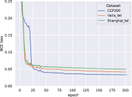
(a)

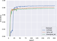
(b)

Figure 2: Learning curves and validation accuracy for $f_{\theta}$.

For the experiments we use the CCCP formulation of the CCP (eq. 8) which considers centroids instead of medians. While there are several possible ways to select a useful number $K$ of clusters, like the Elbow method Yuan and Yang (2019), here we adopt a practical approach consisting of solving the problem with the random assignment baseline method for a number of seeds and choosing the minimal resulting number of clusters as $K$. For the $n=200$ datasets we run all methods for 3 different seeds and report the mean cost with standard deviation and average run times. Since Gurobi requires a run time to be specified because it otherwise can take arbitrarily long for the computation to complete, we set reasonable total run times of 3min for $n=200$ and 15min for the original sizes. If Gurobi times out, we return the last feasible assignment if available. Otherwise, we report the result for that instance as infeasible and set its cost to the average cost of the rnd-NN baseline. Training loss and validation accuracy of our neural scoring function on the different training sets are shown in Figure 2. We evaluate our method in a greedy and a sampling configuration, which we tune on a separate validation set: (g-20-1) stands for 1 greedy rollout for a fraction of $\alpha=0.2$ and (s-25-32) for 32 samples for $\alpha=0.25$.

Datasets

We perform experiments on artificial data and two real world datasets. The artificial data with instances of size $n=200$ we generate based on a GMM. As real world datasets for capacitated spatial clustering we select the well-known Shanghai Telecom (ST) dataset Wang et al. (2019) which contains the locations and user sessions for base stations in the Shanghai region. In order to use it for our CCP task we aggregate the user session lengths per base station as its corresponding weight and remove base stations with only one user or less than 5min of usage in an interval of 15 days as well as outliers far from the city center, leading to a remaining number of $n=2372$ stations. We set the required number of centers to $K=40$. The second dataset we assemble by matching the internet access sessions in the call record data of the Telecom Italia Milan (TIM) dataset Barlacchi et al. (2015) with the Milan cell-tower grid retrieved from OpenCelliD OCID (2021). After pre-processing it contains $n=2020$ points to be assigned to $K=25$ centers. We normalize all weights according to $K$ with a maximum capacity normalization factor of 1.1. The experiments on the real world data are performed in two different settings: The first setting simply executes all methods on the full dataset, while the second setting sub-samples the data in a random local grid to produce 100 test instances of size $n=200$, with weights multiplied by a factor drawn uniformly from the interval [1.5, 4.0) for ST and [2.0, 5.0) for TIM to produce more variation in the required $K$. The exact pre-processing steps and sub-sampling procedure are described in the supplementary.

Baseline Methods

• random: sequentially assigns random labels to points while respecting cluster capacities.

• rnd-NN: selects $K$ random points as cluster centers and sequentially assigns nearest neighbors to these clusters, i.e. points ordered by increasing distance from the center, until no capacity is left.

• topk-NN: similar to random-NN, but instead selects the $K$ points with the largest weight as cluster centers.

• CapKMeans: the capacitated k-means algorithm of Geetha et al. (2009) with ckm++ initialization which outperformed the original topk_weights initialization.

• PACK: the block coordinate descent math-heuristic introduced in Lähderanta et al. (2021) (using Gurobi).

• GB21: the two phase math-heuristic proposed by Gnägi and Baumann (2021) also using the Gurobi solver.

Results

Method	Inertia ($\pm$)	Time (s)	inf. %
random	14.35 (3.77)	0.01	0.0
rnd-NN	7.67 (2.35)	0.01	0.0
topk-NN	7.38 (0.00)	0.01	0.0
GB21	0.98 (0.18)	4.54	1.0
PACK	0.94 (0.14)	14.77	1.0
CapKMeans	1.30 (0.86)	2.19	5.0
NCC (g-20-1)	0.93 (0.01)	1.59	0.0
NCC (s-20-64)	0.92 (0.01)	1.83	0.0

Table 1: Results on generated CCP dataset (100 instances, $n$=200). Best result in bold, second best underlined.

Method	Inertia ($\pm$)	Time (s)	inf. %
Shanghai Telecom (ST)
random	2.61 (0.88)	0.02	0.0
rnd-NN	1.53 (0.30)	0.01	2.3
topk-NN	1.71 (0.00)	0.01	4.0
GB21	0.46 (0.11)	17.49	3.3
PACK	0.57 (0.16)	44.47	8.7
CapKMeans	0.70 (0.22)	4.44	7.0
NCC (g-25-1)	0.52 (0.02)	2.87	0.0
NCC (s-25-32)	0.51 (0.02)	3.53	0.0
Telecom Italia Milan (TIM)
random	3.85 (0.54)	0.02	0.0
rnd-NN	2.00 (0.44)	0.01	1.3
topk-NN	2.12 (0.00)	0.01	0.0
GB21	0.58 (0.10)	14.25	2.3
PACK	0.61 (0.16)	70.09	4.0
CapKMeans	0.68 (0.14)	4.05	2.3
NCC (g-20-1)	0.60 (0.02)	2.44	0.0
NCC (s-25-128)	0.58 (0.01)	4.09	0.0

Table 2: Results on sub-sampled ST and TIM datasets (100 instances, $n$=200). Best result in bold, second best underlined.

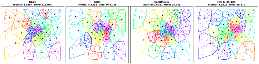
Figure 3: Clusters drawn with their convex hulls for the TIM dataset. Black ”x” markers represent the cluster centers.

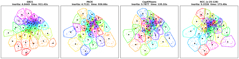
Figure 4: Clusters drawn with their convex hulls for the ST dataset. Black ”x” markers represent the cluster centers.

We evaluate all baselines in terms of inertia, which is defined as the total squared distance of all points to their assigned center. On the generated data (Table 1) our method outperforms all other baselines in terms of inertia while being much faster than all other methods with comparable performance. Furthermore, for three runs with different random seeds our method achieves results with significantly smaller standard deviations and is able to solve all instances within the given time. Results for the sub-sampled datasets are reported in Table 2. On ST our method beats close to all methods in terms of inertia and is only slightly outperformed by GB21 while being 5$\times$ faster. On TIM we achieve similar performance compared to GB21 while being much faster and outperform all other approaches. In particular, we are more than one order of magnitude faster than the next best performing baseline PACK. Furthermore, our method again achieves very small standard deviation for greedy as well as sampling based assignments, showing that it reliably converges to good (local) optima. As expected the random baseline leads to very bad results. The naive baselines rnd-NN and topk-NN are better but still significantly worse than the more advanced methods, achieving inertia which are 3-7 times higher than that of the best method. Compared to CapKMeans NCC leads to improvements of 41%, 37% and 17% respectively for the generated, ST and TIM data while achieving even faster run times, showing the impact of our proposed model adaptations. The inertia and run times for the full datasets are directly reported in the headings of Figures 3 and 4, which display the cluster assignments for Milan and Shanghai, explicitly drawing the convex hull of each cluster for better visualization. While both math-heuristics are able to outperform NCC on these large-scale instances in terms of inertia, our method is close to one order of magnitude faster. Furthermore, the results show that our method is able to find useful cluster structures which especially for TIM are more homogeneous than those of GB21 and show vast improvements compared to CapKMeans.

5.2 Capacitated Vehicle Routing

To show the efficacy of our approach we extend it to a cluster-first-route-second (C1R2) construction method for Capacitated Vehicle Routing Problems (CVRP). The CVRP is an extension of the traveling salesman problem (TSP) in which $K$ capacitated vehicles have to serve the demand of $n$ customers from a fixed depot node Toth and Vigo (2014).

Algorithm Modifications

To adapt our method for the different problem we include an additional MLP in our scoring function, which encodes the depot node, and concatenate the depot embedding with $h_{\operatorname{\mathcal{G}}}$ and $h_{k}$ in eq. 13. In our algorithm we add the depot node to each cluster $k$ during the center update (Algorithm 2, line 22) and add the distance from each node to the depot to the priority weights. After the clustering we use the fast TSP solver provided by VeRyPy Rasku et al. (2019) to route the nodes in each assigned group.

Dataset

To evaluate our algorithm we choose the benchmark dataset of Uchoa et al. (2017) which consists of 100 instances of sizes between 100 and 1000 points sampled according to varying distributions (uniform, clustered, etc.) and with different depot positions and weight distributions. We split the benchmark into three sets of problems with size N1 ($100\leq n<250$), N2 ($250\leq n<500$) and N3 ($500\leq n$).

Baselines

In our experiments we compare against several classical C1R2 approaches: First, the sweep algorithm of Gillett and Miller (1974), which starts a beam at a random point and adds nodes in turn by moving the beam around the depot. We restart the beam at each possible point and run it clock and counter-clock wise. Next, sweep+, which instead of routing nodes in the order in which they were passed by the beam, routes them by solving a TSP with Gurobi. The petal algorithm introduced in Foster and Ryan (1976) creates ”petal” sets by running the sweep algorithm from different starting nodes and then solves a set covering problem with Gurobi to join them. Finally, for comparison (although not C1R2) the powerful auto-regressive neural construction method POMO of Kwon et al. (2020) which is trained with deep reinforcement learning and uses additional instance augmentation techniques. It is evaluated either greedily (g) or with sampling (s) and a beam width of $n$ (size of the instance).

Results

	N1		N2		N3
Method	dist	t (s)	dist	t (s)	dist	t (s)
sweep	57.2	0.65	109.7	2.21	220.7	9.80
	(28.1)		(47.9)		(96.5)
sweep+	40.8	23.9	73.1	105.4	136.4	656.5
	(28.1)		(47.9)		(96.5)
petal	40.4	6.9	72.5	18.2	133.8	86.4
	(28.1)		(47.9)		(96.5)
POMO (g)	33.7	0.1	64.8	0.2	143.7	0.5
	(24.7)		(44.8)		(87.2)
POMO (s)	33.3	1.4	63.8	10.2	136.0	92.3
	(24.7)		(44.7)		(87.1)
NCC (g)	35.9	5.1	67.2	10.2	122.5	29.2
	(24.0)		(43.6)		(84.9)
NCC (s)	35.7	7.1	66.2	18.5	121.5	39.2
	(24.0)		(43.6)		(84.9)
$K_{\text{optimal}}$	(23.8)		(43.5)		(84.5)

Table 3: Results on the Uchoa benchmark. We report the average total distance, time (sec.) and number of vehicles $K$ (in brackets). $K_{\text{optimal}}$ is the target number of vehicles in the benchmark.

As shown in Table 3, our extended approach performs very competitive on the benchmark, beating all C1R2 approaches from the classical literature and being close to POMO on the small and medium sized instances (N1 and N2) while significantly outperforming it on the large instances (N3). Moreover, our method achieves the smallest fleet size of all methods, very close to the optimal fleet size $K_{\text{optimal}}$.

6 Conclusion

This paper presents the first deep learning based approach for the CCP. In experiments on artificial and real world data our method NCC shows competitive performance and fast and robust inference. Moreover, we demonstrate its usefulness as constructive method for the CVRP, achieving promising results on the well-known Uchoa benchmark.

Appendix A Ablation

A.1 Algorithm Design

In this section we present the results of an ablation study to evaluate the usefulness of our adaption to the original capacitated k-means procedure of Geetha et al. Geetha et al. (2009). First, we compare the performance of the original algorithm CapKMeans for different initialization routines. The topk-w initialization is the one originally proposed by Geetha et al., which simply selects the points with the k largest weights as initial cluster centers. We compare it to the k-means++ Arthur and Vassilvitskii (2006) initialization routine, which aims to maximally spread out the cluster centers over the data domain, by sampling a first center uniformly from the data and then sequentially sampling the next center from the remaining data points with a probability equal to the normalized squared distance to the closest already existing center. Moreover, we compare it to our own initialization method ckm++ that includes the weight information into the sampling procedure of k-means++ by simply multiplying the squared distance to the closest existing cluster center by the weight of the data point to sample. Since topk-w is deterministic, the seed points for several random restarts are the same and therefore the procedure is only run once. For a fair comparison we also evaluate k-means++ and ckm++ for one run and report the results in Table 4. We sub-sample some $n=200$ instances from the ST dataset and try to solve them in the different setups. The inertia is measured on the subset of 50 instances for which all five different initializations for CapKMeans produced a feasible result. Those results show, that for a single run without restart, the topk-w method leads to better performance. However, it is directly clear that several restarts can vastly improve the performance and lead to a significantly reduced number of infeasible instances.

The remainder of the ablation study is concerned with evaluating the impact of the other proposed adaptions which led to our full NCC algorithm. The method CapKMeans-alt uses the alternative assignment procedure described in the main paper, which cycles through the centers assigning only one point per turn. Finally, we report the results for the full greedy and sampling procedures as proposed in the main paper. We evaluate all methods with one run for topk-w and eight random restarts for k-means++ and ckm++.

It can be seen that as soon as priorities are computed with the neural scoring function $f_{\theta}$ (for NCC greedy and NCC sampling), the ckm++ initialization outperforms the other two methods, while k-means++ works slightly better in the other two cases. Moreover, we can see that using the neural scoring function significantly improves the algorithm, while simply changing the order of assignment leads to a bit worse results than the original method.

Init	Restarts	Inertia	Avg Run Time (s)	Inf. %
topk-w	1	0.825	1.88	54.0
k-means++	1	0.841	1.91	40.8
ckm++	1	0.860	1.88	44.0
k-means++	8	0.624	2.99	2.0
ckm++	8	0.640	3.02	3.6

Table 4: Ablation on different initialization methods for CapKMeans.

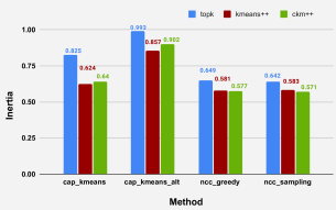
Figure 5: Comparison of different initialization methods and algorithm setups in terms of inertia.

We performed a further ablation study regarding the choice of K for the KNN graph. The results are presented in Figure 6. While run time seems to increase very close to linearly with K, larger K does not necessarily increase performance.

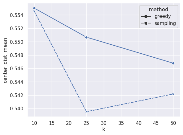
(a)

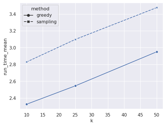
(b)

Figure 6: Inertia and run times for different values of k.

A.2 Generalization to larger and out-of-distribution data

Furthermore, we performed an additional experiment on a diverse selection of the benchmark instances of Stefanello et al. (2015) and present the results in table 5 below. Our model trained on the sub-sampled ST data with $n=200$ is able to work well on problem instances from very different distributions and of significantly larger size.

	NCC (g)		NCC (s)		GB21
Instance	inert.	t (s)	inert.	t (s)	inert.	t (s)
ali535_005	2.257	4.7	2.101	7.6	2.061	5.3
ali535_025	0.291	8.2	0.284	6.9	0.290	61.2
ali535_050	0.166	9.3	0.158	7.4	0.146	364.6
fnl4461_0020	9.961	62.8	9.907	58.8	10.274	241.5
lin318_015	1.446	4.4	1.424	4.3	1.436	4.7
pr2392_020	7.307	30.5	7.641	30.4	7.935	171.2
rl1304_010	7.762	16.4	7.843	16.1	8.447	101.6
sjc3a_300_25	0.011	2.4	0.010	3.9	0.007	16.8
sjc4a_402_30	0.014	5.3	0.014	5.4	0.010	25.3
spain737_74	0.006	2.3	0.005	10.5	0.005	238.4
u724_010	3.891	9.1	3.793	9.0	4.148	9.5
u724_030	1.274	9.5	1.187	9.8	1.174	31.8

Table 5: Results on benchmark instances (format: name_n_k). Our model trained on the sub-sampled ST data with n=200 is able to work well on problem instances from very different distributions and of significantly larger sizes.

Appendix B Data

Apart from the following description of our data related sample and processing steps, we will open source all our data and pre-processing pipelines as jupyter notebooks together with our model code at https://github.com/jokofa/NCC.

B.1 Data Generation

The generated (artificial) data is sampled from a Gaussian Mixture Model where the number $K$ of mixture components is randomly selected between 3 and 12 for each instance. The mean $\mu$ and (diagonal) covariance matrix $\Sigma$ for each component are sampled uniformly from [0, 1]. Weights are also sampled from a standard uniform distribution and re-scaled by a factor of 1.1, i.e. for a problem with $K=3$ components the sum off all weights will be $3/1.1=2.727$. This allows for some flexibility in assigning points to different clusters and is useful to check the ability of the different algorithms to find good assignments in order to minimize the inertia.

B.2 Real World Data

B.2.1 ST

The Shanghai Telecom (ST) dataset Wang et al. (2019) contains the locations and user sessions for base stations in the Shanghai region. In order to use it for our CCP task we aggregate the user session lengths per base station as its corresponding weight and remove base stations with only one user or less than 5min of usage in an interval of 15 days. Furthermore, we remove outliers far from the city center, i.e. outside of the area between latitude (30.5, 31.75) and longitude (120.75, 122), leading to a remaining number of $n=2372$ stations. We set the required number of centers to $K=40$ and normalize the weights with a capacity factor of 1.1.

B.2.2 TIM

The second dataset we assemble by matching the internet access sessions in the call record data of the Telecom Italia Milan (TIM) dataset Barlacchi et al. (2015) with the Milan cell-tower grid retrieved from OpenCelliD OCID (2021). To reduce the number of possible cell towers we only select the ones with LTE support. After pre-processing it contains $n=2020$ points to be assigned to $K=25$ centers. We normalize all weights according to $K$ with a maximum capacity normalization factor of 1.1.

B.3 Data Sub-Sampling

In order to replicate the original data distribution of the full real world datasets on a smaller scale, we employ a sub-sampling procedure. Our main concern is that if one would simply sample randomly from the whole grid, then the relative distance between points in the same cluster for small $n$, e.g. in our case $n_{\text{sub}}=200<<n_{\text{full}}=2020$, would be distorted. Thus, we first select a smaller part of the full point cloud and randomly sub-sample points within that region. To be exact, we first select a random rectangular region of size (0.5*L, 0.5*W), where L and W are the length and width of the full coordinate system in which the original point cloud is contained. Then, we uniformly sample $n_{\text{sub}}$ points from the data points contained in that rectangle. To guarantee sufficient randomness of the sampling process, we require that at least some $n>n_{\text{sub}}$ points are contained in the rectangular region, from which then $n_{\text{sub}}$ points are selected. Moreover, for $n_{\text{sub}}=200$ and $n_{\text{full}}=2020$ with $K=25$ clusters as in the TIM dataset, on average there would only be around 2.5 clusters required per sub sample, which does not present a very intersting clustering task. Thus, we rescale the weights of each sub-sample by a factor drawn uniformly from the interval [1.5, 4.0) for ST and [2.0, 5.0) for TIM to produce more variation in the required number of clusters $K$. An exemplary plot of the procedure is given in Figure 7.

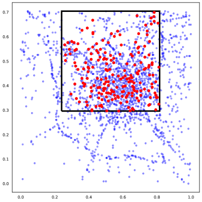
Figure 7: Example plot of the used sub-sampling procedure on the TIM dataset. A rectangle (black) of size (0.5*L, 0.5*W) at a random position within the coordinate system is selected. Then $n$ data points (red) are sampled uniformly from within the rectangle. Finally, the weights of the chosen points are re-scaled.

Appendix C Training and Hyperparameters

Here we report the training regime and hyperparameters used to learn our neural scoring function:
Our model is implemented in PyTorch Paszke et al. (2019) version 1.11. We use $L=4$ GNN layers, an embedding dimension of $d_{\text{emb}}=256$ and a dimension of $d_{\text{h}}=256$ for all hidden layers of the neural networks. Furthermore, GELU activations Hendrycks and Gimpel (2016) and layer norm (LN) Ba et al. (2016) is employed. The model is trained for 200 epochs with a mini-batch size of 128 using the Adam optimizer Kingma and Ba (2014) and a learning rate of $\lambda=0.001$ which is nearly halved every 40 epochs by multiplying it with a factor of $0.55$. Moreover, we clip the gradient norm above $0.5$. The global seed used for training is 1234. As $\mathcal{K}$ for the KNN graph generation we use $\mathcal{K}=25$ for the artificial data and the TIM dataset while $\mathcal{K}=16$ worked better for the ST data. The corresponding models are trained with training and validation sets with instances of size $n=200$, either generated artificial data or independently sub-sampled datasets for TIM and ST. The size of the training sets is 4000 for the artificial data and 4900 for both real world datasets. The targets are created by solving the respective instances with the two phase math-heuristic proposed by Gnägi and Baumann (2021) which uses the Gurobi solver Gurobi Optimization, LLC (2023). To solve these datasets in a reasonable time, we set the maximum time for the solver to 32 seconds for the artificial data and 200 seconds for TIM and ST.

For the NCC algorithm we do a small non-exhaustive grid search on the validation data to select the fraction of re-prioritized points $\alpha$ in {0.05, 0.10, 0.15, 0.20, 0.25} and the number of samples for the sampling method in {32, 64, 128}. The chosen values are directly reported in the result tables in the main paper.

Ethical Statement

There are no ethical issues.

References

- Arthur and Vassilvitskii [2006] David Arthur and Sergei Vassilvitskii. k-means++: The advantages of careful seeding. Technical report, Stanford, 2006.
- Ba et al. [2016] Jimmy Lei Ba, Jamie Ryan Kiros, and Geoffrey E Hinton. Layer normalization. arXiv preprint arXiv:1607.06450, 2016.
- Barlacchi et al. [2015] Gianni Barlacchi, Marco De Nadai, Roberto Larcher, Antonio Casella, Cristiana Chitic, Giovanni Torrisi, Fabrizio Antonelli, Alessandro Vespignani, Alex Pentland, and Bruno Lepri. A multi-source dataset of urban life in the city of milan and the province of trentino. Scientific data, 2(1):1–15, 2015.
- Celebi et al. [2013] M Emre Celebi, Hassan A Kingravi, and Patricio A Vela. A comparative study of efficient initialization methods for the k-means clustering algorithm. Expert systems with applications, 40(1):200–210, 2013.
- Ester et al. [1996] Martin Ester, Hans-Peter Kriegel, Jörg Sander, Xiaowei Xu, et al. A density-based algorithm for discovering clusters in large spatial databases with noise. In kdd, volume 96, pages 226–231, 1996.
- Foster and Ryan [1976] Brian A Foster and David M Ryan. An integer programming approach to the vehicle scheduling problem. Journal of the Operational Research Society, 27(2):367–384, 1976.
- Geetha et al. [2009] S Geetha, G Poonthalir, and PT Vanathi. Improved k-means algorithm for capacitated clustering problem. INFOCOMP Journal of Computer Science, 8(4):52–59, 2009.
- Genevay et al. [2019] Aude Genevay, Gabriel Dulac-Arnold, and Jean-Philippe Vert. Differentiable deep clustering with cluster size constraints. arXiv preprint arXiv:1910.09036, 2019.
- Gillett and Miller [1974] Billy E Gillett and Leland R Miller. A heuristic algorithm for the vehicle-dispatch problem. Operations research, 22(2):340–349, 1974.
- Gnägi and Baumann [2021] Mario Gnägi and Philipp Baumann. A matheuristic for large-scale capacitated clustering. Computers & operations research, 132:105304, 2021.
- Grubesic et al. [2014] Tony H Grubesic, Ran Wei, and Alan T Murray. Spatial clustering overview and comparison: Accuracy, sensitivity, and computational expense. Annals of the Association of American Geographers, 104(6):1134–1156, 2014.
- Guo et al. [2017] Xifeng Guo, Xinwang Liu, En Zhu, and Jianping Yin. Deep clustering with convolutional autoencoders. In International conference on neural information processing, pages 373–382. Springer, 2017.
- Gurobi Optimization, LLC [2023] Gurobi Optimization, LLC. Gurobi Optimizer Reference Manual. https://www.gurobi.com, 2023.
- Hendrycks and Gimpel [2016] Dan Hendrycks and Kevin Gimpel. Gaussian error linear units (gelus). arXiv preprint arXiv:1606.08415, 2016.
- Jain et al. [1999] Anil K Jain, M Narasimha Murty, and Patrick J Flynn. Data clustering: a review. ACM computing surveys (CSUR), 31(3):264–323, 1999.
- Kingma and Ba [2014] Diederik P Kingma and Jimmy Ba. Adam: A method for stochastic optimization. arXiv preprint arXiv:1412.6980, 2014.
- Kwon et al. [2020] Yeong-Dae Kwon, Jinho Choo, Byoungjip Kim, Iljoo Yoon, Youngjune Gwon, and Seungjai Min. Pomo: Policy optimization with multiple optima for reinforcement learning. Advances in Neural Information Processing Systems, 33:21188–21198, 2020.
- Lähderanta et al. [2021] Tero Lähderanta, Teemu Leppänen, Leena Ruha, Lauri Lovén, Erkki Harjula, Mika Ylianttila, Jukka Riekki, and Mikko J Sillanpää. Edge computing server placement with capacitated location allocation. Journal of Parallel and Distributed Computing, 153:130–149, 2021.
- LeCun and Cortes [2010] Yann LeCun and Corinna Cortes. MNIST handwritten digit database. 2010.
- Lloyd [1982] Stuart Lloyd. Least squares quantization in pcm. IEEE transactions on information theory, 28(2):129–137, 1982.
- Lorena and Furtado [2001] Luiz Antonio Nogueira Lorena and João Carlos Furtado. Constructive genetic algorithm for clustering problems. Evolutionary Computation, 9(3):309–327, 2001.
- MacQueen [1967] J MacQueen. Classification and analysis of multivariate observations. In 5th Berkeley Symp. Math. Statist. Probability, pages 281–297, 1967.
- Manduchi et al. [2021] Laura Manduchi, Kieran Chin-Cheong, Holger Michel, Sven Wellmann, and Julia Vogt. Deep conditional gaussian mixture model for constrained clustering. Advances in Neural Information Processing Systems, 34:11303–11314, 2021.
- McLachlan and Basford [1988] Geoffrey J McLachlan and Kaye E Basford. Mixture models: Inference and applications to clustering, volume 38. M. Dekker New York, 1988.
- Morris et al. [2019] Christopher Morris, Martin Ritzert, Matthias Fey, William L Hamilton, Jan Eric Lenssen, Gaurav Rattan, and Martin Grohe. Weisfeiler and leman go neural: Higher-order graph neural networks. In Proceedings of the AAAI conference on artificial intelligence, volume 33, pages 4602–4609, 2019.
- Mulvey and Beck [1984] John M Mulvey and Michael P Beck. Solving capacitated clustering problems. European Journal of Operational Research, 18(3):339–348, 1984.
- Negreiros and Palhano [2006] Marcos Negreiros and Augusto Palhano. The capacitated centred clustering problem. Computers & operations research, 33(6):1639–1663, 2006.
- Negreiros et al. [2022] Marcos J Negreiros, Nelson Maculan, Augusto WC Palhano, Albert EF Muritiba, and Pablo LF Batista. Capacitated clustering models to real life applications. artificial intelligence (AI), 3:8, 2022.
- OCID [2021] OCID. Opencellid. https://opencellid.org, 2021. Accessed: 2021/08/04.
- Osman and Christofides [1994] Ibrahim H Osman and Nicos Christofides. Capacitated clustering problems by hybrid simulated annealing and tabu search. International Transactions in Operational Research, 1(3):317–336, 1994.
- Ozawa [1985] Kazumasa Ozawa. A stratificational overlapping cluster scheme. Pattern recognition, 18(3-4):279–286, 1985.
- Paszke et al. [2019] Adam Paszke, Sam Gross, Francisco Massa, Adam Lerer, James Bradbury, Gregory Chanan, Trevor Killeen, Zeming Lin, Natalia Gimelshein, Luca Antiga, et al. Pytorch: An imperative style, high-performance deep learning library. Advances in neural information processing systems, 32, 2019.
- Raghavan et al. [2019] S Raghavan, Mustafa Sahin, and F Sibel Salman. The capacitated mobile facility location problem. European Journal of Operational Research, 277(2):507–520, 2019.
- Rasku et al. [2019] Jussi Rasku, Tommi Kärkkäinen, and Nysret Musliu. Meta-survey and implementations of classical capacitated vehicle routing heuristics with reproduced results. Toward Automatic Customization of Vehicle Routing Systems, 2019.
- Ren et al. [2022] Yazhou Ren, Jingyu Pu, Zhimeng Yang, Jie Xu, Guofeng Li, Xiaorong Pu, Philip S Yu, and Lifang He. Deep clustering: A comprehensive survey. arXiv preprint arXiv:2210.04142, 2022.
- Ross and Soland [1977] G Terry Ross and Richard M Soland. Modeling facility location problems as generalized assignment problems. Management Science, 24(3):345–357, 1977.
- Scheuerer and Wendolsky [2006] Stephan Scheuerer and Rolf Wendolsky. A scatter search heuristic for the capacitated clustering problem. European Journal of Operational Research, 169(2):533–547, 2006.
- Stefanello et al. [2015] Fernando Stefanello, Olinto CB de Araújo, and Felipe M Müller. Matheuristics for the capacitated p-median problem. International Transactions in Operational Research, 22(1):149–167, 2015.
- Tian et al. [2014] Fei Tian, Bin Gao, Qing Cui, Enhong Chen, and Tie-Yan Liu. Learning deep representations for graph clustering. In Proceedings of the AAAI Conference on Artificial Intelligence, volume 28, 2014.
- Toth and Vigo [2014] Paolo Toth and Daniele Vigo. Vehicle routing: problems, methods, and applications. SIAM, 2014.
- Uchoa et al. [2017] Eduardo Uchoa, Diego Pecin, Artur Pessoa, Marcus Poggi, Thibaut Vidal, and Anand Subramanian. New benchmark instances for the capacitated vehicle routing problem. European Journal of Operational Research, 257(3):845–858, 2017.
- Vaswani et al. [2017] Ashish Vaswani, Noam Shazeer, Niki Parmar, Jakob Uszkoreit, Llion Jones, Aidan N Gomez, Łukasz Kaiser, and Illia Polosukhin. Attention is all you need. Advances in neural information processing systems, 30, 2017.
- Wagstaff et al. [2001] Kiri Wagstaff, Claire Cardie, Seth Rogers, Stefan Schrödl, et al. Constrained k-means clustering with background knowledge. In Icml, volume 1, pages 577–584, 2001.
- Wang et al. [2019] Shangguang Wang, Yali Zhao, Jinlinag Xu, Jie Yuan, and Ching-Hsien Hsu. Edge server placement in mobile edge computing. Journal of Parallel and Distributed Computing, 127:160–168, 2019.
- Xie et al. [2016] Junyuan Xie, Ross Girshick, and Ali Farhadi. Unsupervised deep embedding for clustering analysis. In International conference on machine learning, pages 478–487. PMLR, 2016.
- Yang et al. [2017] Bo Yang, Xiao Fu, Nicholas D Sidiropoulos, and Mingyi Hong. Towards k-means-friendly spaces: Simultaneous deep learning and clustering. In international conference on machine learning, pages 3861–3870. PMLR, 2017.
- Yuan and Yang [2019] Chunhui Yuan and Haitao Yang. Research on k-value selection method of k-means clustering algorithm. J, 2(2):226–235, 2019.
- Zhang et al. [2021] Hongjing Zhang, Tianyang Zhan, Sugato Basu, and Ian Davidson. A framework for deep constrained clustering. Data Mining and Knowledge Discovery, 35(2):593–620, 2021.