Wellposedness, exponential ergodicity and numerical approximation of fully super-linear McKean–Vlasov SDEs and associated particle systems

Abstract

We study a class of McKean–Vlasov Stochastic Differential Equations (MV-SDEs) with drifts and diffusions having super-linear growth in measure and space – the maps have general polynomial form but also satisfy a certain monotonicity condition. The combination of the drift’s super-linear growth in measure (by way of a convolution) and the super-linear growth in space and measure of the diffusion coefficient requires novel technical elements in order to obtain the main results. We establish wellposedness, propagation of chaos (PoC), and under further assumptions on the model parameters, we show an exponential ergodicity property alongside the existence of an invariant distribution. No differentiability or non-degeneracy conditions are required.

Further, we present a particle system based Euler-type split-step scheme (SSM) for the simulation of this type of MV-SDEs. The scheme attains, in stepsize, the strong error rate $1/2$ in the non-path-space root-mean-square error metric and we demonstrate the property of mean-square contraction. Our results are illustrated by numerical examples including: estimation of PoC rates across dimensions, preservation of periodic phase-space, and the observation that taming appears to be not a suitable method unless strong dissipativity is present.

Keywords: McKean–Vlasov equations, split-step methods, ergodicity, interacting particle systems, super-linear growth in measure

1 Introduction

In this work, we analyze a class of McKean–Vlasov Stochastic Differential Equations (MV-SDEs) having drift and diffusion components of convolution type, akin to the porous media equation or interaction kernel modelling, which allows for super-linear growth in measure and space in both coefficients – one may think of the super-linearity as higher-order polynomials under some additional conditions regulating spatial and measure radial growth. We work with MV-SDE dynamics of the form

$$\mathrm{d}X_{t} =\big{(}v(X_{t},\mu_{t}^{X})+b(t,X_{t},\mu_{t}^{X})\big{)}\mathrm{d}t+\overline{\sigma}(t,X_{t},\mu_{t}^{X})\mathrm{d}W_{t},\quad X_{0}\in L^{m}(\mathbb{R}^{d}),\leavevmode\nobreak\ m>2$$ (1.1)

$$\textrm{where }\leavevmode\nobreak\ v(x,\mu)=\int_{\mathbb{R}^{d}}f(x-y)\mu(\mathrm{d}y)+u(x,\mu),\quad\overline{\sigma}(t,x,\mu)=\sigma(t,x,\mu)+\int_{\mathbb{R}^{d}}f_{\sigma}(x-y)\mu(\mathrm{d}y).$$ (1.2)

Above, $\mu_{t}^{X}$ denotes the law of the solution process $X$ at time $t$, $L^{m}(\mathbb{R}^{d})$ is the space of $\mathcal{F}_{0}$-measurable random variables with finite $m$-th moments, $W$ is a multidimensional Brownian motion, $u,b,\sigma$ and $f,f_{\sigma}$ are measurable maps. Critically, $f,f_{\sigma},u,\sigma$ are maps of super-linear growth but not assumed to be differentiable and $\bar{\sigma}$ may degenerate. The function $u$ in $v$ allows to incorporate measure dependencies other than convolution type.

In terms of a modelling perspective in the context of particle dynamics, (1.1)-(1.2) model the dynamics of particle motion where the particle is affected by different sources of forcing. The map $u$ represents a multi-well gradient potential confining the particle (and the source of super-linear growth in the spatial component) and the convolution map $f$ contains information on the forces affecting the particles (attractive, repulsive), see [40, 66, 3]. As argued in [40], under certain assumptions, $v$ (and $f$) adds inertia to the particle’s dynamic in turn affecting its exit time from a domain of attraction (by accelerating or delaying it) and alters exit locations [40, 30, 3] (also [26]). To motivate the study of equations with a (nonlinear) convolution term $(f_{\sigma}\ast\mu)(\cdot):=\int_{\mathbb{R}^{d}}f_{\sigma}(\cdot-y)\mu(\mathrm{d}y)$ in the diffusion component, which is the main feature of our work, we first mention [38]. There, a Cucker–Smale model incorporating random communication is rewritten as a Cucker–Smale model with multiplicative noise (the diffusion coefficient has the form $\left(\mathbb{E}[X_{t}]-X_{t}\right)=\int_{\mathbb{R}^{d}}(X_{t}-y)\mu_{t}(\mathrm{d}y)$), which helps to stabilize flocking states as the effect of the noise diminishes the closer the particles concentrate around their mean; see also [4]. These works give a clear motivation to analyze convolution type diffusion maps (diffusions whose strength depends on the density) – also [31] studies a kinetic flocking model with a more general distance potential (communication rate) function than [38]. In addition, [13] considers general stochastic systems of interacting particles with Brownian noise to study models for the collective behavior (swarming) – more particularly, [13, Section 1.2.2] highlights several open-question model extensions to nonlinear diffusion coefficients (though beyond the scope of this work). The recent works [20, 14] investigate consensus-based optimization (CBO) methods for solving high-dimensional nonlinear unconstrained minimization problems. A CBO scheme updates the particle’s position in an iterative manner to explore the optimization landscape. There, particles far away from the equilibrium state are expected to exhibit more exploration (i.e., the noise level should be larger) compared to particles close to it. Inspired by the above discussed works, we offer a new class of MV-SDEs adding a new element in the diffusion coefficient by means of a reversion to the population mean expressed through a fully non-Lipschitz $f_{\sigma}\ast\mu$ significantly beyond the linear interaction diffusion coefficients studied in the mentioned works.

More generally, the motivation to study this class of MV-SDEs and associated interacting particle systems is to present a unified framework to address wellposedness and establish properties useful for downstream applications. For instance, from emerging models of mean-field type in neuroscience [32], understating particle motion and exit times [40, 41, 66, 3, 71], parametric inference [35] (also [7, 25]) is an important consideration. We also point to Section 4 and 5 of [46] for a variety of general interacting systems that are subsumed by our class. Our results can also be viewed as an addition to the literature on granular media type equations as studied in [21, 37, 61].

The existence and uniqueness of solutions to MV-SDEs, in a strong and weak sense, has been extensively studied, see e.g., [22, 64, 58, 50, 44, 53, 62, 19, 47, 55] and references therein, but none cover the setting presented here. To the best of our knowledge, the existence and uniqueness of strong solutions to equations with super-linear growth in the measure component of the drift and the diffusion has not been addressed in general. There exist various works considering super-linearly growing coefficients (in state) but do not incorporate $f$ or $f_{\sigma}$, see e.g., [55, 69, 49] and its references. In [3] the authors deal with a super-linear $f$, $f_{\sigma}\equiv 0$, and a (unbounded) uniformly Lipschitz continuous $\sigma$, and derive wellposedness (i.e., existence and uniqueness of a strong solution) and large deviation results. Further, [73] allows for a setting similar to ours but requires upfront strong dissipativity and non-degeneracy. Their aim was to study ergodicity, nonetheless, it is unclear how to adapt their methodology if working with the goal of proving wellposedness over $[0,T]$ under milder conditions. From the initial work [3], our goal is to develop a general framework to study (1.1)-(1.2) in terms of wellposedness (over $[0,T]$), with a super-linearly growing $\sigma$ and $f_{\sigma}$, ergodicity and approximation schemes.

Our first main contribution concerns wellposedness and propagation of chaos (PoC) results for the finite time horizon $[0,T]$ case. The critical nontrivial hurdle of this setting is in establishing $L^{p}$-moment bounds for $p>2$ under the presence of the super-linear growths of $f$, $f_{\sigma}$ and $\sigma$ – this issue appears solely due to the simultaneous presence of nonlinearities (in space and measure) in the drift and diffusion, otherwise techniques like those of [3] or [49] would suffice. To overcome this hurdle, we introduce a new condition dubbed ‘additional symmetry’, which is new in the literature (to the best of our knowledge). For a quick perspective, we suggest the reader glance at Lemma A.1 and A.2 (in Appendix) and the proof of Theorem 2.5 to see how one deals with the convolution terms and to note the importance of the ‘additional symmetry’ condition – a discussion on this latter condition is presented in Remark 2.6. We also address a propagation of chaos result [64, 56, 33, 27, 30] for this class. We show the interacting particle system, obtained by replacing $\mu^{X}$ by the system’s $N$-particle empirical distribution, recovers the original MV-SDE in the particle limit $N\to\infty$. Under a very mild higher-integrability assumption, a convergence rate is obtained.

Our second main contribution addresses another key element of MV-SDE theory which is the existence and uniqueness of an invariant probability measure and exponential convergence to it (i.e., ergodicity). This is a particularly important property in applications involving statistical inference [7] (usually in neuroscience [1, 17, 16, 34, 36]) or associated long-term behaviour connected to metastability [66, 67, 3].

We extend the wellposedness result to the infinite time horizon and then analyze the long-time behaviour of our class of MV-SDEs. We prove an exponential ergodicity property and the existence of an invariant measure. The proof arguments loosely follow those of [69, 43, 52] and, critically, do not make use of Lyapunov functions or the Krylov–Bogoliubov machinery. In fact, to reach this type of results for McKean–Vlasov equations, the Krylov–Bogoliubov machinery is not a suitable one due to the nonlinearities of the involved semi-group and hence the classical tightness argument does not apply, see discussions in [69, 43, 52]. On the other hand, Lyapunov function arguments are also difficult to use for the particular MV-SDE class in this manuscript – this is due to the presence of a convolution operator with a function $f$ (and $f_{\sigma}$) that is not of linear growth. If the polynomial power was on the convolution term, instead of inside it, then the Lyapunov machinery would successfully carry through [52]. For our case, and as mentioned before, an additional difficulty arises solely due to the simultaneous presence of the super-linear growth in $f$, $f_{\sigma}$ and $\sigma$. The ergodicity/invariance proof arguments of [69, 43, 52] leverage the completeness of the space of probability measures with finite second order moments to identify the invariant measure, but our wellposedness result requires a sufficiently integrable initial condition (with strictly more than second order moments). This issue leads to a more involved proof – see discussion prior to Theorem 2.7.

The third main contribution of this work is a numerical method to approximate (1.1)-(1.2) over $[0,T]$ via its interacting particle system. Most of our theoretical results are only proven for the finite time case, but we successfully apply the scheme for the long-term simulation of a particle system as well. There are presently many studies for numerical methods allowing super-linear spatial growth of drifts (and diffusions): Euler type methods, e.g., taming [29], time-adaptive [60], semi-implicit methods [23], projection methods [8]; Milstein type methods e.g., [48, 59, 6, 5] with some allowing super-linear $\sigma$ in space. There are variations on the assumptions, but all these contributions require drifts and diffusions to be globally Lipschitz continuous in measure (with respect to the Wasserstein distance with quadratic cost). Two recent contributions [51, 57] allow for weaker continuity conditions than Lipschitz for the coefficients but require a linear growth in space and measure. Only [24] allows for general super-linear growth in $f,u$ but still limits $\overline{\sigma}$ to satisfy Lipschitz assumptions – we detail below the differences between [24] and this manuscript in more detail.

The scheme we propose here belongs to the split-step method (SSM) class. Such schemes were analyzed for MV-SDEs with drifts which are Lipschitz in measure and diffusion coefficients satisfying a uniform Lipschitz condition [23]; the scheme appeared originally in [42] for standard SDEs. We follow the strategy of approximating (in time) the interacting particle system associated with the MV-SDE and using a quantitative propagation of chaos (PoC) convergence result, see [15] and [60, 59, 29] for earlier uses of this strategy. From a methodological point of view, the convergence proof of our numerical scheme is different from any used to study MV-SDE numerical schemes in the literature; our highly-non-linear setting forces us to draw on the stochastic $C$-stability and $B$-consistency mechanics proposed in [10]. Its use in the context of numerical schemes for MV-SDEs and interacting particle systems is novel in the literature – except for the very recent [12] that studies higher order strong scheme for MV-SDE under non-differentiability conditions using a randomisation method. In [12], the authors work with generic Lipschitz assumptions and need to change the underpinning error norms to cope with the complexity arising from the randomization step due to an explicit non-differentiability assumption on the drift coefficient. Our approach and requirements differ, and so does the analysis (albeit similar at points). We show that it is possible to work directly with the concepts of [10] to deal with the interacting particle system, see Section 2.5 – we emphasize that the main goal of the analysis is to guarantee that core moment estimates are uniformly independent of the number of particles $N$ of the interacting system (but may depend on the initial system’s underlying dimension $d$). As is common in the MV-SDE literature, results from the SDE numerics literature on super-linear growth do not carry over to the MV-SDE one.

Closest to our work with regards to the SSM is [24], where the authors propose an SSM scheme similar to the one here for interacting particle systems that have (1.1) (with $f_{\sigma}\equiv 0$ and $\sigma$ globally Lipschitz continuous in space and measure) as limit. There they overcome the barrier of super-linear growth in space and measure for the drift (that [29, 60, 23] do not), but work with a diffusion component of Lipschitz type; the focus of [24] is solely the analysis of the numerical scheme and not wellposedness or ergodicity. Our setting is more involved those of [24, 23] and requires novel proof techniques – here, drawing from [10], specifically due to the simultaneous super-linearity in drift and diffusion. In [24], bounds for higher order moments of the discrete process obtained by the time-stepping scheme can be developed by commonly used assumptions like $(\mathbf{A}^{u},\leavevmode\nobreak\ \mathbf{A}^{\sigma})$ below. For our situation, the super-linearity in the diffusion coefficient (in space and measure) is controlled by a drift satisfying a suitable one-sided Lipschitz condition. However, the simultaneous appearance of nonlinearities in the diffusion and the nonlinear convolution $f\ast\mu$ in the drift causes difficulties. This is the reason why, for the scheme in this manuscript, only $L^{2}$-moment bounds were established, and the proof methodology takes recourse in the stochastic $C$-stability and $B$-consistency mechanics of [10] (which does not require to establish bounds for higher order moments of the SSM). It remains unclear how to obtain higher moments (even with the help of the new additional symmetry assumption).

In terms of findings, we show the scheme achieves a strong convergence rate of order $1/2$ and establish sufficient conditions for mean-square stability in the sense of [23, Definition 2.8]. We present several numerical examples of interest and for comparison we implement, without proof, two intuitive versions of taming methods [29, 59]. Our examples show the SSM to perform very well for the approximation of a solution to (1.1) on $[0,T]$ in an $L^{2}$-sense or the approximation for the ergodic distribution. The numerical results using taming are mixed but suffice to highlight which version can be expected to converge (theoretically). We show a surprising numerical divergence finding for taming given the choice of initial condition and which does not appear when using the SSM (see our Section 3.1) – this confirms the SSM as a stable/robust choice of scheme for this class. The SSM is shown to preserve periodicity of phase-space. Lastly, we provide a numerical example with the aim of estimating the PoC rate across dimensions and which highlights a gap in the literature: we observe the rate of [56, 27] (not applicable to our setting) instead of those in [33, 18] (which are used to prove our PoC result). Future research focuses on the study of uniform in-time PoC results and strong convergence rates for the SSM on $[0,\infty)$.

Organization of the paper. Section 2 contains: notations, framework, wellposedness and ergodicity results, the particle approximation and the propagation of chaos statement, and the numerical scheme alongside associated convergence results. Several numerical examples are provided in Section 3. They cover the non-dissipative case in short and long time horizons; approximation of the invariant distribution; preservation of periodicity in phase-space and numerical estimation of PoC rates across dimension. All proofs are postponed to Section 4. Generic auxiliary results are given in the Appendix.

2 Main results

2.1 Notation and Spaces

We follow the notation and framework set in [3, 23]. Let $\mathbb{N}$ be the set of natural numbers starting at $0$ and for $a,b\in\mathbb{N}$ with $a\leq b$, define $\llbracket a,b\rrbracket:=[a,b]\cap\mathbb{N}=\{a,\ldots,b\}$. For $x,y\in\mathbb{R}^{d}$ denote the inner product of vectors by $\langle x,y\rangle$, and $|x|=(\sum_{j=1}^{d}x_{j}^{2})^{1/2}$ the Euclidean distance. Let $\mathbbm{1}_{B}$ be the indicator function of the set $B\subset\mathbb{R}^{d}$. For a matrix $A\in\mathbb{R}^{d\times l}$ we denote by $A^{\intercal}$ its transpose and its Frobenius norm by $|A|=\textrm{Trace}\{AA^{\intercal}\}^{1/2}$.

We introduce on the measurable space $(\mathbb{R}^{d},\mathcal{B}(\mathbb{R}^{d}))$, where $\mathcal{B}(\mathbb{R}^{d})$ denotes the Borel $\sigma$-field over $\mathbb{R}^{d}$, the set of all probability measures $\mathcal{P}(\mathbb{R}^{d})$ and its subset $\mathcal{P}_{r}(\mathbb{R}^{d})$ of those with finite $r\in[1,\infty)$ moment. The space $\mathcal{P}_{r}(\mathbb{R}^{d})$ is a Polish space when endowed with the Wasserstein distance

$$W^{(r)}(\mu,\nu):=\inf_{\pi\in\Pi(\mu,\nu)}\Big{(}\int_{\mathbb{R}^{d}\times\mathbb{R}^{d}}|x-y|^{r}\pi(\mathrm{d}x,\mathrm{d}y)\Big{)}^{\frac{1}{r}},\quad\mu,\nu\in\mathcal{P}_{r}(\mathbb{R}^{d}),$$

where $\Pi(\mu,\nu)$ is the set of couplings for $\mu$ and $\nu$ such that $\pi\in\Pi(\mu,\nu)$ is a probability measure on $\mathbb{R}^{d}\times\mathbb{R}^{d}$ with $\pi(\cdot\times\mathbb{R}^{d})=\mu$ and $\pi(\mathbb{R}^{d}\times\cdot)=\nu$. For a given function $f$ with domain on $\mathbb{R}^{d}$, $x\in\mathbb{R}^{d}$ with $\mu\in\mathcal{P}(\mathbb{R}^{d})$, the convolution operator $\ast$ is defined as $(f\ast\mu)(x):=\int_{\mathbb{R}^{d}}f(x-y)\mu(\mathrm{d}y)$. Let our probability space be a completion of $(\Omega,\mathbb{F},\mathcal{F},\mathbb{P})$ with $\mathbb{F}=\{\mathcal{F}_{t}\}_{t\geq 0}$ being the natural filtration of the Brownian motion $W=(W^{1},\ldots,W^{l})$ with $l$-dimensions, augmented with a sufficiently rich sub $\sigma$-algebra $\mathcal{F}_{0}$ independent of $W$. We denote by $\mathbb{E}[\cdot]=\mathbb{E}^{\mathbb{P}}[\cdot]$ the usual expectation operator with respect to $\mathbb{P}$.

We consider some finite terminal time $T<\infty$ and use the following notation for spaces, which are standard in the literature [29, 23]. For $p\geq 1$, we denote by $L^{p}\left(\Omega,\mathcal{F}_{t},\mathbb{P};\mathbb{R}^{d}\right)$ the space of $\mathbb{R}^{d}$-valued, $\mathcal{F}_{t}$-measurable random variables $X$ with finite $|X|_{L^{p}(\Omega,\mathcal{F}_{t},\mathbb{P};\mathbb{R}^{d})}$-norm given by $|X|_{L^{p}(\Omega,\mathcal{F}_{t},\mathbb{P};\mathbb{R}^{d})}=\mathbb{E}\left[|X|^{p}\right]^{1/p}$. Define $\mathbb{S}^{p}([0,T])$, as the space of $\mathbb{R}^{d}$-valued, $\mathbb{F}$-adapted, continuous processes $Z$ with finite $\|Z\|_{\mathbb{S}^{p}}$-norm defined as $\|Z\|_{\mathbb{S}^{p}}=\mathbb{E}\left[\sup_{0\leqslant t\leqslant T}|Z_{t}|^{p}\right]^{1/p}$.

Throughout the text, $C$ denotes a generic positive real-valued constant that may depend on the problem’s data, and change from line to line, but is always independent of the constants $h,M,N$ (associated with the numerical scheme and specified below).

2.2 Framework

Let $v:\mathbb{R}^{d}\times\mathcal{P}_{2}(\mathbb{R}^{d})\to\mathbb{R}^{d}$, $b:[0,\infty)\times\mathbb{R}^{d}\times\mathcal{P}_{2}(\mathbb{R}^{d})\to\mathbb{R}^{d}$ and $\overline{\sigma}:[0,\infty)\times\mathbb{R}^{d}\times\mathcal{P}_{2}(\mathbb{R}^{d})\to\mathbb{R}^{d\times l}$ be measurable maps. The MV-SDE of interest of this work is Equation (1.1) (for some $m>2$), where $\mu_{t}^{X}$ denotes the law of the process $X$ at time $t$, i.e., $\mu_{t}^{X}=\mathbb{P}\circ X_{t}^{-1}$. We make the following assumptions on the coefficients.

Assumption 2.1.

The functions $b$ and $\sigma$ are $1/2$-Hölder continuous in time, uniformly in $x\in\mathbb{R}^{d}$ and $\mu\in\mathcal{P}_{2}(\mathbb{R}^{d})$ and $\sup_{t\in[0,\infty)}\big{(}|b(t,0,\delta_{0})|+|\sigma(t,0,\delta_{0})|\big{)}\leq L$, for some constant $L\geq 0$.
$(\mathbf{A}^{b})$ Let $b$ be uniformly Lipschitz continuous in the sense that there exists $L_{(b)}^{(1)},\leavevmode\nobreak\ L_{(b)}^{(3)}\geq 0$ and $L_{(b)}^{(2)}\in\mathbb{R}$ such that for all $t\in[0,\infty)$, $x,x^{\prime}\in\mathbb{R}^{d}$ and $\mu,\mu^{\prime}\in\mathcal{P}_{2}(\mathbb{R}^{d})$ we have that

$$|b(t,x,\mu)-b(t,x^{\prime},\mu^{\prime})|^{2} \leq L_{(b)}^{(1)}\big{(}|x-x^{\prime}|^{2}+\big{(}W^{(2)}(\mu,\mu^{\prime})\big{)}^{2}\big{)},$$

$$\langle x-x^{\prime},b(t,x,\mu)-b(t,x^{\prime},\mu^{\prime})\rangle \leq L_{(b)}^{(2)}|x-x^{\prime}|^{2}+L_{(b)}^{(3)}\big{(}W^{(2)}(\mu,\mu^{\prime})\big{)}^{2}.$$

$(\mathbf{A}^{u},\leavevmode\nobreak\ \mathbf{A}^{\sigma})\leavevmode\nobreak\$ Let $u,\sigma$ satisfy: there exist $L^{(1)}_{(u\sigma)}\in\mathbb{R}$, and $L^{(2)}_{(u\sigma)},L^{(3)}_{(u\sigma)},L^{(4)}_{(u\sigma)},q_{1}\geq 0$ such that for all $t\in[0,\infty)$, $x,x^{\prime}\in\mathbb{R}^{d}$ and $\mu,\mu^{\prime}\in\mathcal{P}_{2}(\mathbb{R}^{d})$, with $m>2$ in (1.1), we have that

$$\color[rgb]{0,0,0}\langle x-x^{\prime},u(x,\mu)-u(x^{\prime},\mu^{\prime})\rangle+2(m-1)|\sigma(t,x,\mu)-\sigma(t,x^{\prime},\mu^{\prime})|^{2} \color[rgb]{0,0,0}\leq L^{(1)}_{(u\sigma)}|x-x^{\prime}|^{2}+L^{(2)}_{(u\sigma)}\big{(}W^{(2)}(\mu,\mu^{\prime})\big{)}^{2},$$ (2.1)

$$|u(x,\mu)-u(x^{\prime},\mu)|+|\sigma(t,x,\mu)-\sigma(t,x^{\prime},\mu)| \leq L^{(3)}_{(u\sigma)}(1+|x|^{q_{1}}+|x^{\prime}|^{q_{1}})|x-x^{\prime}|,$$ (2.2)

$$|u(x,\mu)-u(x,\mu^{\prime})|^{2}+|\sigma(t,x,\mu)-\sigma(t,x,\mu^{\prime})|^{2} \leq L^{(4)}_{(u\sigma)}\big{(}W^{(2)}(\mu,\mu^{\prime})\big{)}^{2}.$$

$(\mathbf{A}^{f},\leavevmode\nobreak\ \mathbf{A}^{f_{\sigma}})\leavevmode\nobreak\$ Let $f,f_{\sigma}$ satisfy: there exist $L^{(1)}_{(f)},L^{(3)}_{(f)}\in\mathbb{R}$, and $L^{(2)}_{(f)},q_{2}\geq 0$, such that for all $x,x^{\prime}\in\mathbb{R}^{d}$, $2<p\leq m$, we have that

$$\langle x-x^{\prime},f(x)-f(x^{\prime})\rangle+2(m-1)|f_{\sigma}(x)-f_{\sigma}(x^{\prime})|^{2} \leq L^{(1)}_{(f)}|x-x^{\prime}|^{2}, \textrm{(One-sided Lipschitz, monotonicity condition)},$$

$$|f(x)-f(x^{\prime})|+|f_{\sigma}(x)-f_{\sigma}(x^{\prime})| \leq L^{(2)}_{(f)}(1+|x|^{q_{2}}+|x^{\prime}|^{q_{2}})|x-x^{\prime}|, \textrm{(Locally Lipschitz)},$$

$$f(x) =-f(-x),$$ (Odd function),

$$\color[rgb]{0,0,0}(|x|^{p-2}-|x^{\prime}|^{p-2})\langle x+x^{\prime},f(x-x^{\prime})\rangle \color[rgb]{0,0,0}\leq L^{(3)}_{(f)}(|x|^{p}+|x^{\prime}|^{p}), \color[rgb]{0,0,0}\textrm{(Additional symmetry)}.$$

Assume the normalization $f(0)=f_{\sigma}(0)=0$. Lastly, and for convenience, we set $q=\max\{q_{1},q_{2}\}\geq 0.$

Remark 2.2 (Time dependency for $u$).

To avoid added complexity to an already complex work, we do not address time-dependence on $u$. A close inspection of the proof for wellposedness and convergence of the numerical scheme shows that as long as the time dependence does not interfere with constraints imposed by Assumption 2.1 the results will hold. Additionally one would require a $1/2$-Hölder continuity property for the function.

All elements in the above assumption are standard, except the ‘additional symmetry’ restriction. The ‘additional symmetry’ is a new type of restriction which we have not found previously in the literature and we discuss it in more detail at several points in the text, in particular, in Remark 2.6.

This condition is trivially satisfied when $d=1$ (see (2.3)) or when the function is Lipschitz. We next provide a non-trivial example in $d>1$ for $f$ satisfying the ‘extra symmetry’ condition.

Example 2.3.

For $x\in\mathbb{R}^{d}$ define $f(x)=-x|x|^{2}$. Then, for any $p>2$, $x,y\in\mathbb{R}^{d}$ it holds that

$$(|x|^{p-2}-|y|^{p-2})\langle x+y,-(x-y)|x-y|^{2}\rangle =-(|x|^{p-2}-|y|^{p-2})(|x|^{2}-|y|^{2})|x-y|^{2}\leq 0,$$

and the conclusion follows from the monotonicity of the polynomial function.

Remark 2.4 (Implied properties).

Let Assumption 2.1 hold with $m>2$. We provide the following estimates for some positive constant $C$ which may change line by line, which are derived using the one-sided Lipschitz condition and Young’s inequality (see [24, Remark 2.2] for details). For all $t\in[0,T]$, $x,x^{\prime},z\in\mathbb{R}^{d}$ and $\mu,\mu^{\prime}\in\mathcal{P}_{2}(\mathbb{R}^{d})$, we have

$$\langle x,f(x)\rangle+2(m-1)|f_{\sigma}(x)|^{2} \leq L^{(1)}_{(f)}|x|^{2},\quad\color[rgb]{0,0,0}\langle x,u(x,\mu)\rangle+(m-1)|\sigma(t,x,\mu)|^{2}\leq C\big{(}1+|x|^{2}+(W^{(2)}(\mu,\delta_{0}))^{2}\big{)},$$

$$\langle x-x^{\prime},u(x,\mu)-u(x^{\prime},\mu^{\prime})\rangle \leq C\big{(}|x-x^{\prime}|^{2}+(W^{(2)}(\mu,\mu^{\prime}))^{2}\big{)},\quad\langle x,b(t,x,\mu)\rangle\leq C(1+|x|^{2}+(W^{(2)}(\mu,\delta_{0}))^{2}),$$

$$\langle x-x^{\prime},v(x,\mu)-v(x^{\prime},\mu)\rangle \leq(L^{(1)}_{(u\sigma)}+L^{(1)}_{(f)})|x-x^{\prime}|^{2},\quad|b(t,x,\mu)|^{2}\leq C\big{(}1+|x|^{2}+(W^{(2)}(\mu,\delta_{0}))^{2}\big{)}$$

$$|\overline{\sigma}(t,x,\mu)|^{2} \leq 2|\sigma(t,x,\mu)|^{2}+2\big{|}\int_{\mathbb{R}^{d}}f_{\sigma}(x-y)\mu(\mathrm{d}y)\big{|}^{2}\leq 2|\sigma(t,x,\mu)|^{2}+2\int_{\mathbb{R}^{d}}|f_{\sigma}(x-y)|^{2}\mu(\mathrm{d}y).$$

Let $f:\mathbb{R}\rightarrow\mathbb{R}$ be an odd-function satisfying the one-sided Lipschitz condition, then $f$ satisfies the additional symmetry condition, i.e., for $x,y\in\mathbb{R},x\neq y,p\geq 2$, we have

$$(|x|^{p-2}-|y|^{p-2})\langle x+y,f(x-y)\rangle =\frac{(|x|^{p-2}-|y|^{p-2})(x+y)}{x-y}\langle x-y,f(x-y)\rangle\leq C(|x|^{p}+|y|^{p}).$$ (2.3)

The following decomposition is crucial for the remaining parts of this work for $x\in\mathbb{R}^{d}$, $m\geq p>2$, $\mu\in\mathcal{P}_{m}(\mathbb{R}^{d})$ it holds that

$$\int_{\mathbb{R}^{d}}\int_{\mathbb{R}^{d}} |x|^{p-2}\langle x,f(x-y)\rangle\mu(\mathrm{d}y)\mu(\mathrm{d}x)=\frac{1}{2}\int_{\mathbb{R}^{d}}\int_{\mathbb{R}^{d}}\langle|x|^{p-2}x-|y|^{p-2}y,f(x-y)\rangle\mu(\mathrm{d}y)\mu(\mathrm{d}x)$$

$$=\frac{1}{2}\int_{\mathbb{R}^{d}}\int_{\mathbb{R}^{d}}\langle(|x|^{p-2}x-|x|^{p-2}y)+(|x|^{p-2}y-|y|^{p-2}y),f(x-y)\rangle\mu(\mathrm{d}y)\mu(\mathrm{d}x)$$

$$=\int_{\mathbb{R}^{d}}\int_{\mathbb{R}^{d}}\big{(}\tfrac{1}{2}|x|^{p-2}\langle x-y,f(x-y)\rangle+\tfrac{1}{4}(|x|^{p-2}-|y|^{p-2})\langle x+y,f(x-y)\rangle\big{)}\mu(\mathrm{d}y)\mu(\mathrm{d}x).$$ (2.4)

The decomposition in (2.4) along with $(\mathbf{A}^{f},\leavevmode\nobreak\ \mathbf{A}^{f_{\sigma}})\leavevmode\nobreak\$ will be used to incorporate the nonlinearity of $f_{\sigma}$.

2.3 Existence, uniqueness and ergodicity of the MV-SDE

Let us start by stating the wellposedness result of MV-SDE (1.1).

Theorem 2.5 (Wellposedness).

Let Assumption 2.1 hold with $m>2q+2$, then there exists a unique strong solution $X$ to MV-SDE (1.1) satisfying the following estimates: For some constant $C>0$, we have a pointwise estimate

$$\sup_{t\in[0,T]}\mathbb{E}\big{[}|X_{t}|^{\widetilde{m}}\big{]}\leq C\left(1+\mathbb{E}[|X_{0}|^{\widetilde{m}}]\right)e^{CT},\qquad\textrm{for any }\leavevmode\nobreak\ \widetilde{m}\in[2,m].$$

The proof of the wellposedness theorem is postponed to Section 4.1.

Remark 2.6 (On the ‘additional symmetry’ restriction).

The critical element of the proof for this result, is the difficulty in establishing (finite) bounds for higher order moments of the solution process. The ‘additional symmetry’ assumption is a technical condition without which we were not able to establish $L^{p}$-moment bounds for $p>2$ (and $d>1$) – proving $L^{2}$-moment bounds or uniqueness of the solution is straightforward and the condition is not needed. The requirement of ‘additional symmetry’ stems solely from having a super-linearly growing $\sigma$, $f_{\sigma}$ and a super-linear growth of the convolution term appearing in the drift. If either of them is of linear growth (or $d=1$), then the ‘additional symmetry’ condition can be removed and the results hold.

The strategy used in [3] to establish $L^{p}$-moment bounds, working with Assumption 2.1 but with a linearly growing $\sigma$, is to bound $\mathbb{E}\big{[}|X_{t}|^{2p}\big{]}$ via

$$\mathbb{E}\big{[}|X_{t}|^{2p}\big{]} \leq C\big{(}\mathbb{E}\big{[}\big{|}X_{t}-\mathbb{E}[X_{t}]\big{|}^{2p}\big{]}+\mathbb{E}\big{[}|X_{t}|^{2}\big{]}^{p}\big{)},$$

and then noticing that

$$\mathbb{E}\big{[}\big{|}X_{t}-\mathbb{E}[X_{t}]\big{|}^{2p}\big{]}=\int_{\mathbb{R}^{d}}\big{|}x-\int_{\mathbb{R}^{d}}y\mu_{t}(\mathrm{d}y)\big{|}^{2p}\mu_{t}(\mathrm{d}x) \leq\int_{\mathbb{R}^{d}}\int_{\mathbb{R}^{d}}|x-y|^{2p}\mu_{t}(\mathrm{d}y)\mu_{t}(\mathrm{d}x)=\mathbb{E}\big{[}|X_{t}-\tilde{X}_{t}|^{2p}\big{]},$$

with $\tilde{X}$ an independent copy of $X$ driven by its independent Brownian motion, see Lemma A.1 and Lemma A.2 for extra details. This trick allows to deal with the convolution term, employing its symmetry, (see Lemma A.2), but does not give control of the super-linear diffusion. To be precise, Itô’s formula applied to $|X-\tilde{X}|^{2p}$ forces one to use the polynomial growth condition on $\sigma$ (2.2), which involves higher moments, instead of (2.1).

Without the trick described above, and following more classical approaches [59, Theorem 2.1], it is possible to control the super-linear growth of $\sigma$ in space (via (2.1)) but it is unclear how to simultaneously control the super-linear growth of the convolution terms in a tractable way (the tricks of Lemma A.1 and Lemma A.2 do not carry over).

All in all, there is competition between the growths of $f$ and $\sigma$, $f_{\sigma}$, and neither just described technique is adequate to establish $L^{p}$-moment estimates. The ‘additional symmetry’ condition offsets this difficulty. See details in the proof in Section 4.1. Lifting this restriction is left as an open question.

Next, recall the constants $q,m$ from Assumption 2.1, we consider the long-time behaviour, an exponential ergodic property and the existence of an invariant measure for the MV-SDEs of interest. We point the reader to [69, 70] for a review on recent results. To this end, we need to estimate differences of (1.1) with different initial conditions and introduce the associated nonlinear semigroup.

Define the nonlinear semigroup $(P^{*}_{s,t})$ for $0\leq s\leq t<\infty$ on $\mathcal{P}_{\ell}(\mathbb{R}^{d}),\leavevmode\nobreak\ \ell>2q+2$ by setting $P^{*}_{s,t}\mu:=\textrm{Law}(X_{s,t})$ and $X_{s,\cdot}$ is the solution to (1.1) starting from time $s$ such that $\textrm{Law}(X_{s,s})=\mu$. Note that standard literature sets the semigroup in $\mathcal{P}_{2}(\mathbb{R}^{d})$ but in this manuscript Theorem 2.5 requires higher integrability of the initial condition and working with $\mathcal{P}_{\ell}(\mathbb{R}^{d}),\ell>2q+2$ reflects that. In the notation introduced earlier, we have $P^{*}_{0,t}\mu_{0}^{X}:=\mu_{t}^{X}$, and more generally $P^{*}_{s,t}=P^{*}_{s,r}P^{*}_{r,t}$ for $s\leq r\leq t$. Crucially, if $b$ and $\sigma$ in (1.1) are independent of time, then $P^{*}_{s,t}=P^{*}_{0,t-s}$ (see [69]).

We say that $\bar{\mu}$ is an invariant distribution of the semigroup $P^{*}$ if $P^{*}_{0,t}\bar{\mu}=\bar{\mu}$ holds for all $t\geq 0$. The semigroup satisfies an ergodic property if there exists $\widehat{\mu}\in\mathcal{P}_{\ell}(\mathbb{R}^{d})$ such that $\lim_{t\to\infty}P^{*}_{0,t}\nu=\widehat{\mu}$ (weakly) for all $\nu$ (at this point, we leave unclear the space where $\nu$ belongs to). In the proof of the theorem below, we show that the property holds true for any $\nu\in\mathcal{P}_{2\ell-2}(\mathbb{R}^{d})\subset\mathcal{P}_{\ell}(\mathbb{R}^{d}),\leavevmode\nobreak\ \ell>2q+2$ with convergence taking place through the $W^{(\ell)}$-metric in $\mathcal{P}_{2\ell-2}(\mathbb{R}^{d})$. These results differ from those in [69] and the proof requires further care.

Theorem 2.7 (Contraction, exponential ergodicity property and invariance).

Let the Assumptions of Theorem 2.5 hold with $m>4q+2$. Assume that there exist constants $L^{(1)}_{(bu\sigma)},L^{(3)}_{(bu\sigma)}\geq 0$, and $L^{(2)}_{(bu\sigma)}\in\mathbb{R}$ such that for all $t\in[0,\infty)$, $x\in\mathbb{R}^{d}$ and $\mu\in\mathcal{P}_{2}(\mathbb{R}^{d})$ we have that

$$\big{\langle}x,u(x,\mu)+b(t,x,\mu)\big{\rangle}+(m-1)|\sigma(t,x,\mu)|^{2} \leq L^{(1)}_{(bu\sigma)}+L^{(2)}_{(bu\sigma)}|x|^{2}+L^{(3)}_{(bu\sigma)}\big{(}W^{(2)}(\mu,\delta_{0})\big{)}^{2}.$$

Then the following three assertions hold:

1. For $\mu,\nu\in\mathcal{P}_{\ell}(\mathbb{R}^{d})$, with $2q+2<\ell$, $L^{(1),+}_{(f)}=\max\{L^{(1)}_{(f)},0\}$ and $\rho_{1}=2L_{(b)}^{(2)}+2L_{(b)}^{(3)}+2L^{(1)}_{(u\sigma)}+2L^{(2)}_{(u\sigma)}+4L^{(1),+}_{(f)}$, $t\in[0,T],\leavevmode\nobreak\ T<\infty$, we have

   $$\big{(}W^{(2)}(P^{*}_{0,t}\mu,P^{*}_{0,t}\nu)\big{)}^{2}\leq e^{\rho_{1}t}\big{(}W^{(2)}(\mu,\nu)\big{)}^{2}.$$ (2.5)

2. Let $\mu\in\mathcal{P}_{\ell}(\mathbb{R}^{d})$ with $2q+2<\ell\leq m$, $\rho_{2,\ell}=\ell(L^{(2)}_{(bu\sigma)}+L^{(3)}_{(bu\sigma)}+2L^{(1),+}_{(f)}+L^{(3)}_{(f)}/2)+(\ell-2)/\ell$, $t\in[0,T],\leavevmode\nobreak\ T<\infty$. Then for some constant $C$ depending on $\ell,\leavevmode\nobreak\ L^{(1)}_{(bu\sigma)}$ and $\sup_{t}|b(t,0,\delta_{0})|$, but independent of time $t$, we have

   $$\big{(}W^{(\ell)}(P^{*}_{0,t}\mu,\delta_{0})\big{)}^{\ell}\leq e^{\rho_{2,\ell}t}\big{(}W^{(\ell)}(\mu,\delta_{0})\big{)}^{\ell}+\frac{C}{\rho_{2,\ell}}(e^{\rho_{2,\ell}t}-1)\mathbbm{1}_{\rho_{2,\ell}\neq 0}+Ct\mathbbm{1}_{\rho_{2,\ell}=0}.$$ (2.6)

3. Assume further that the functions $b,\sigma$ are independent of time and that $\rho_{1},\rho_{2,2\ell-2}<0$ with $1+m/2\geq\ell>2q+2$. Then (2.5) yields exponential contraction, (2.6) yields bounded orbits, and there exists a unique invariant measure $\bar{\mu}\in\mathcal{P}_{\ell}(\mathbb{R}^{d})$, such that, for any $t>0$ and $\nu_{0}\in\mathcal{P}_{2\ell-2}(\mathbb{R}^{d})$ we have

   $$W^{(2)}(P^{*}_{0,t}\bar{\mu},\bar{\mu})=0\qquad\textrm{and}\qquad W^{(2)}(P^{*}_{0,t}\nu_{0},\bar{\mu})\leq e^{\rho_{1}t/2}W^{(2)}\big{(}\nu_{0},\bar{\mu}\big{)}.$$

   In fact, for any $\nu_{0}\in\mathcal{P}_{2\ell-2}(\mathbb{R}^{d})$ we have $\lim_{t\to\infty}W^{(\ell)}(P_{0,t}^{*}\nu_{0},\bar{\mu})=0$.

The proof is postponed to Section 4.2 and a quick inspection shows that for statement 1 and 2, one only needs $\ell>2q+2$. Strictly speaking, the requirement for the initial distribution $\nu_{0}\in\mathcal{P}_{2\ell-2}(\mathbb{R}^{d})$ is only needed for the final statement. The mechanism of choice for the proof is inspired by [69, Theorem 3.1]. In essence, (2.6) can be interpreted as the existence of a ‘non-expanding orbit’, i.e., there is a ‘bounded orbit’ and the exponential contractivity of the Wasserstein metric (under $\rho_{1},\rho_{2,2\ell-2}<0$) in (2.7) yields that all orbits are bounded – for further considerations see [52].

It is unclear how the Lyapunov functional techniques used in [43], [52] (or [39]) can be applied to the class of MV-SDEs of this work (it is the super-linear growth of $f$ in the convolution term that causes problems; if the polynomial growth is on the convolution integral instead of $f$ then the theory carries over) – we leave this issue for future research.

2.4 Particle approximation of the MV-SDE

We now turn to the particle approximation of the MV-SDE with the ultimate goal of establishing a working numerical scheme for the equation. All results here are only concerned with the finite-time case.

As in [15, 60, 23], we approximate the MV-SDE (1.1) (driven by the Brownian motion $W$) by an interacting particle system, i.e., an $N$-dimensional system of $\mathbb{R}^{d}$-valued interacting particles. Let $i\in\llbracket 1,N\rrbracket$ and consider $N$ particles $(X_{t}^{i,N})_{t\in[0,T]}$ with independent and identically distributed (i.i.d.) initial data ${X}_{0}^{i,N}=X_{0}^{i}$ (an independent copy of $X_{0}$) satisfying the $(\mathbb{R}^{d})^{N}$-valued SDE

$$\mathrm{d}{X}_{t}^{i,N}=\big{(}v(X_{t}^{i,N},\mu^{X,N}_{t})+b(t,{X}_{t}^{i,N},\mu^{X,N}_{t})\big{)}\mathrm{d}t+\overline{\sigma}(t,{X}_{t}^{i,N},\mu^{X,N}_{t})\mathrm{d}W_{t}^{i},\quad X^{i,N}_{0}=X_{0}^{i},$$ (2.7)

where $\mu^{X,N}_{t}(\mathrm{d}x):=\frac{1}{N}\sum_{j=1}^{N}\delta_{X_{t}^{j,N}}(\mathrm{d}x)$ with $\delta_{x}$ being the Dirac measure at $x\in\mathbb{R}^{d}$, and $W^{i}$ being independent Brownian motions (also independent of the Brownian motion appearing in (1.1)). We introduce similarly to [24, Remark 2.4] the auxiliary maps $V$, and $\hat{\Sigma}$ to view (2.7) as a system in $\mathbb{R}^{Nd}$.

Lemma 2.8 (Properties of the particle system as a system in $\mathbb{R}^{Nd}$).

Define $V:\mathbb{R}^{Nd}\to\mathbb{R}^{Nd}$, $\hat{\Sigma}:[0,T]\times\mathbb{R}^{Nd}\to\mathbb{R}^{Nd\times Nl}$ by $V(x^{N})=\big{(}\ldots,v(x^{i,N},\mu^{x,N}),\ldots\big{)},$ and $\hat{\Sigma}(t,x^{N})=\big{(}\ldots,\overline{\sigma}(t,x^{i,N},\mu^{x,N}),\ldots\big{)}$ with $x^{N}=(x^{1,N},\ldots,x^{N,N})\in\mathbb{R}^{Nd}$, $\leavevmode\nobreak\ t\in[0,T]$.

Then, under Assumption 2.1 with $m>2$, for any $x^{N},y^{N}\in\mathbb{R}^{Nd}$ with corresponding empirical measures $\mu^{x,N}=\tfrac{1}{N}\sum_{j=1}^{N}\delta_{x^{j,N}}$, and $\mu^{y,N}=\tfrac{1}{N}\sum_{j=1}^{N}\delta_{y^{j,N}}$, the functions $V,\leavevmode\nobreak\ \hat{\Sigma}$ also satisfy a monotonicity condition (see first item of $(\mathbf{A}^{f},\leavevmode\nobreak\ \mathbf{A}^{f_{\sigma}})\leavevmode\nobreak\$ in Assumption 2.1) in $\mathbb{R}^{Nd}$ (with constants independent of $N$).

Proof.

From Assumption 2.1, Remark 2.4 and Jensen’s inequality, we deduce, for all $x^{N},y^{N}\in\mathbb{R}^{Nd},\leavevmode\nobreak\ t\in[0,T]$,

$$\langle x^{N}-y^{N},V(x^{N})-V(y^{N})\rangle+\frac{(m-1)}{2}|\hat{\Sigma}(t,x^{N})-\hat{\Sigma}(t,y^{N})|^{2}$$

$$\leq\frac{1}{2N}\sum_{i=1}^{N}\sum_{j=1}^{N}\big{\langle}(x^{i,N}-x^{j,N})-(y^{i,N}-y^{j,N}),f(x^{i,N}-x^{j,N})-f(y^{i,N}-y^{j,N})\big{\rangle}$$

$$\quad+\sum_{i=1}^{N}\Big{(}\big{\langle}x^{i,N}-y^{i,N},u(x^{i,N},\mu^{x,N})-u(y^{i,N},\mu^{y,N})\big{\rangle}+(m-1)|\sigma(t,x^{i,N},\mu^{x,N})-\sigma(t,y^{i,N},\mu^{y,N})|^{2}\Big{)}$$

$$\quad+\frac{m-1}{N}\sum_{i=1}^{N}\sum_{j=1}^{N}|f_{\sigma}(x^{i,N}-x^{j,N})-f_{\sigma}(y^{i,N}-y^{j,N})|^{2}\leq C|x^{N}-x^{N}|^{2},$$

where $C>0$ is independent of $N$.

∎

Propagation of chaos (PoC). In order to show that the particle approximation (2.7) is effective to approximate the underlying MV-SDE, we present a pathwise propagation of chaos result (convergence as the number of particles increases). To do so, we introduce the system of non interacting particles

$$\mathrm{d}X_{t}^{i}=\big{(}v(X_{t}^{i},\mu^{X^{i}}_{t})+b(t,X_{t}^{i},\mu^{X^{i}}_{t})\big{)}\mathrm{d}t+\overline{\sigma}(t,X_{t}^{i},\mu^{X^{i}}_{t})\mathrm{d}W_{t}^{i},\quad t\in[0,T],$$ (2.8)

which are (decoupled) MV-SDEs with i.i.d. initial conditions $X_{0}^{i}$ (an independent copy of $X_{0}$). Since the $X^{i}$’s are independent, $\mu^{X^{i}}_{t}=\mu^{X}_{t}$ for all $i$ (and $\mu^{X}_{t}$ the marginal law of the solution to (1.1)). We are interested in the strong error-type metrics for the numerical approximation and the relevant PoC result for our case is given in the next theorem, the proof is postponed to Section 4.

Theorem 2.9 (Propagation of Chaos).

Let the Assumptions of Theorem 2.5 hold for some $m>2(q+1)$. Let $X^{i}$ be the solution to (2.8) in the sense of Theorem 2.5. Then, there exists a unique solution $X^{i,N}$ to (2.7) and for any $1\leq p\leq m$ there exists $C>0$ independent of $N$ such that

$$\sup_{i\in\llbracket 1,N\rrbracket}\sup_{t\in[0,T]}\mathbb{E}\big{[}|X^{i,N}_{t}|^{p}\big{]}\leq C(1+\mathbb{E}\big{[}\,|X_{0}|^{p}\big{]}).$$

Moreover, suppose that $m>2(q+1)$ and $m>4$, then we have the following convergence result

$$\sup_{i\in\llbracket 1,N\rrbracket}\sup_{t\in[0,T]}\mathbb{E}\big{[}|X_{t}^{i,N}-X_{t}^{i}|^{2}\big{]}\leq C\begin{cases}N^{-1/2},&d<4,\\ N^{-1/2}\log N,&d=4,\\ N^{-\frac{2}{d+4}},&d>4.\end{cases}$$ (2.9)

This result shows that the particle approximation will converge to the MV-SDE with a given rate. Therefore, to establish convergence of our numerical scheme to the MV-SDE (in a strong sense), we only need to show that the discrete-time version of the particle system converges to the “true” particle system.

2.5 $C$-stability and $B$-consistency for the particle system

Before introducing our numerical scheme and the corresponding strong convergence result, we first present a definition of $C$-stability and $B$-consistency for the particle system. The following definitions and methodologies are modifications of the original work in [10] tailored to the present particle system setting. The probability space in this section supports (at least) the $N$ driving Brownian motions of the particle system and the filtration corresponds to the enlarged filtration generated by all Brownian motions augmented by a rich enough $\sigma$-algebra $\mathcal{F}_{0}$.

Definition 2.10.

Let $h\in(0,T]$ be the stepsize and $\Psi_{i}:\mathbb{R}^{d}\times\mathcal{P}_{2}(\mathbb{R}^{d})\times[0,T]\times\Omega\rightarrow\mathbb{R}^{d}$ for all $i\in\llbracket 1,N\rrbracket$ be a mapping satisfying the following measurability and integrability condition: For every $t,t+h\in[0,T],\leavevmode\nobreak\ h\in(0,1)$ and $X=(X^{1},\ldots,X^{N})\in L^{2}\left(\Omega,\mathcal{F}_{t},\mathbb{P};\mathbb{R}^{Nd}\right)$ , $\mu\in\mathcal{P}_{2}(\mathbb{R}^{d})$ it holds

$$\Psi_{i}(X^{i},\mu,t,h)\in L^{2}\big{(}\Omega,\mathcal{F}_{t+h},\mathbb{P};\mathbb{R}^{d}\big{)},\quad\Psi=(\Psi_{1},\ldots,\Psi_{N}).$$ (2.10)

Then, for $M\in\mathbb{N},Mh=T,\leavevmode\nobreak\ k\in\llbracket 0,M-1\rrbracket$, $t_{k}=kh$, we say that a particle system $\hat{X}_{k}^{N}=(\hat{X}_{k}^{1,N},\ldots,\hat{X}_{k}^{N,N})\in\mathbb{R}^{Nd}$ is generated by the stochastic one-step method $(\Psi,h,\xi)$ with initial condition $\xi=(\xi^{1},\ldots,\xi^{N})\in L^{2}\left(\Omega,\mathcal{F}_{0},\mathbb{P};\mathbb{R}^{Nd}\right)$, $\Psi=(\Psi_{1},\ldots,\Psi_{N})$ , if

$$\hat{X}_{k+1}^{i,N}=\Psi_{i}(\hat{X}_{k}^{i,N},\hat{\mu}_{k}^{X,N},t_{k},h),\quad\hat{\mu}_{k}^{X,N}(\mathrm{d}x)=\frac{1}{N}\sum_{j=1}^{N}\delta_{\hat{X}_{k}^{j,N}}(\mathrm{d}x),$$

$$\hat{X}_{0}^{i,N}=\xi^{i},\quad i\in\llbracket 1,N\rrbracket.$$

We call $\Psi$ the one-step map of the method.

Definition 2.11.

A stochastic one-step method $(\Psi,h,\xi)$ is called stochastically $C$-stable if there exists a constant $C>0$ and a parameter $\eta\in(1,\infty)$ such that for all $t,t+h\in[0,T],\leavevmode\nobreak\ h>0$ and all random variables $X_{t}^{i,N},Z_{t}^{i,N}\in L^{2}\left(\Omega,\mathcal{F}_{t},\mathbb{P};\mathbb{R}^{d}\right),\leavevmode\nobreak\ i\in\llbracket 1,N\rrbracket$, from identically distributed particle systems with their empirical measures $\mu_{t}^{X,N},\leavevmode\nobreak\ \mu_{t}^{Z,N}\in\mathcal{P}_{2}(\mathbb{R}^{d})$, it holds

$$\mathbb{E}\Big{[}\left|\mathbb{E}\big{[}\Psi_{i}(X_{t}^{i,N},\mu_{t}^{X,N},t,h)-\Psi_{i}(Z_{t}^{i,N},\mu_{t}^{Z,N},t,h)\mid\mathcal{F}_{t}\big{]}\right|^{2}\Big{]}$$

$$\qquad+\eta\mathbb{E}\Big{[}\left|\left(\mathrm{id}-\mathbb{E}\big{[}\cdot\mid\mathcal{F}_{t}\big{]}\right)\big{(}\Psi_{i}(X_{t}^{i,N},\mu_{t}^{X,N},t,h)-\Psi_{i}(Z_{t}^{i,N},\mu_{t}^{Z,N},t,h)\big{)}\right|^{2}\Big{]}$$

$$\qquad\qquad\qquad\qquad\leq\left(1+Ch\right)\mathbb{E}\big{[}|X_{t}^{i,N}-Z_{t}^{i,N}|^{2}\big{]}+Ch\big{(}W^{(2)}(\mu_{t}^{X,N},\mu_{t}^{Z,N})\big{)}^{2}.$$

Here, and in what follows we denote by $\left(\mathrm{id}-\mathbb{E}\left[\cdot\mid\mathcal{F}_{t}\right]\right)Y=Y-\mathbb{E}\left[Y\mid\mathcal{F}_{t}\right]$ the projection of an $\mathcal{F}_{t+h}$-measurable random variables $Y$ orthogonal to the conditional expectation $\mathbb{E}\left[\cdot\mid\mathcal{F}_{t}\right]$.

Definition 2.12.

Let $X^{i,N},\leavevmode\nobreak\ i\in\llbracket 1,N\rrbracket$, be the unique strong solution to (2.7), with $\mu^{X,N}$ being the corresponding empirical measure. A stochastic one-step method $(\Psi,h,\xi)$ is called stochastically $B$-consistent of order $\gamma>0$ if there exists a constant $C>0$ such that for all $t,t+h\in[0,T],\leavevmode\nobreak\ h\in(0,1)$, it holds

$${\mathbb{E}\Big{[}\left|\mathbb{E}\big{[}X_{t+h}^{i,N}-\Psi_{i}(X_{t}^{i,N},\mu^{X,N}_{t},t,h)\mid\mathcal{F}_{t}\big{]}\right|^{2}\Big{]}} \leq Ch^{2\gamma+2},$$

$${\mathbb{E}\Big{[}\left|\left(\mathrm{id}-\mathbb{E}\big{[}\cdot\mid\mathcal{F}_{t}\big{]}\right)\big{(}X_{t+h}^{i,N}-\Psi_{i}(X_{t}^{i,N},\mu^{X,N}_{t},t,h)\big{)}\right|^{2}\Big{]}} \leq Ch^{2\gamma+1}.$$

Next, we show the convergence results based on the definitions above.

Lemma 2.13.

Let $(\Psi,h,\xi)$ be a stochastically $C$-stable one-step method with some $\eta\in(1,\infty)$. For the particle system $X^{i,N}$, given by (2.7) with its empirical distribution $\mu^{X,N}$, we have

$$\sup_{n\in\llbracket 0,M\rrbracket}\sup_{i\in\llbracket 1,N\rrbracket}\mathbb{E}\big{[}|X^{i,N}_{n}-\hat{X}^{i,N}_{n}|^{2}\big{]}\leq e^{CT}\bigg{[}\mathbb{E}\big{[}|X^{i,N}_{0}-\xi^{i}|^{2}\big{]}$$

$$\quad+\sum_{k=1}^{M}\sup_{i\in\llbracket 1,N\rrbracket}\bigg{(}(1+h^{-1})\mathbb{E}\Big{[}\big{|}\mathbb{E}\big{[}X^{i,N}_{k}-\Psi_{i}(X^{i,N}_{k-1},\mu^{X,N}_{k-1},t_{k-1},h)\mid\mathcal{F}_{t_{k-1}}\big{]}\big{|}^{2}\Big{]}$$

$$\quad\qquad\qquad+C_{\eta}\leavevmode\nobreak\ \mathbb{E}\Big{[}\Big{|}\left(\mathrm{id}-\mathbb{E}\big{[}\cdot\mid\mathcal{F}_{t_{k-1}}\big{]}\right)\big{(}X^{i,N}_{k}-\Psi_{i}(X^{i,N}_{k-1},\mu^{X,N}_{k-1},t_{k-1},h)\big{)}\Big{|}^{2}\Big{]}\bigg{)}\bigg{]}$$

where $C_{\eta}=1+(\eta-1)^{-1}$ and $\hat{X}^{i,N}_{n}$ denotes the particles generated by $(\Psi,h,\xi)$, with $X^{i,N}_{k}=X^{i,N}_{t_{k}}$, $\mu^{X,N}_{k}=\mu^{X,N}_{t_{k}}$, $t_{k}=kh$ for all $k\in\llbracket 0,M\rrbracket$.

Theorem 2.14.

Let the stochastic one-step method $(\Psi,h,\xi)$ be stochastically $C$-stable and stochastically $B$-consistent of order $\gamma>0$. If $\xi^{i}=X_{0}^{i,N}=\hat{X}_{0}^{i,N}$, then there exists a constant $C$ independent of $N,h$ such that

$$\sup_{n\in\llbracket 0,M\rrbracket}\sup_{i\in\llbracket 1,N\rrbracket}\mathbb{E}\big{[}|X_{n}^{i,N}-\hat{X}_{n}^{i,N}|^{2}\big{]}\leq Ch^{2\gamma},$$

where $X^{i,N}$ denotes the exact solution to (2.7) and $\hat{X}^{i,N}$ is the particle generated by $(\Psi,h,\xi)$. In particular, $(\Psi,h,\xi)$ is strongly convergent of order $\gamma$.

2.6 The numerical scheme

The split-step method (SSM) proposed here follows the steps of [24] and will be re-casted accordingly. The critical difficulty arises from the simultaneous appearance of the convolution component in $v$ (1.1) and the super-linear diffusion coefficient. The presence of both nonlinearities is the main hindrance to proving moment bounds of order $p>2$ for the numerical scheme. Therefore, we rely on the $C$-stability and $B$-consistency methodology, as this approach does not require proving moment stability of higher order for the numerical scheme. This is in stark contrast to the techniques used in [24], where the time-stepping scheme has stable moments of higher order (depending on the regularity of the initial data) and strong convergence rates are proven without employing the $C$-stability and $B$-consistency procedure. Here, we wish to emphasize that even with the symmetry condition it is unclear how to prove $L^{p}$-moment bounds of the numerical scheme for $p>2$.

Definition 2.15 (Definition of the SSM).

Let Assumption 2.1 hold, let $h$ satisfy (2.14) and let $M\in\mathbb{N}$ such that $Mh=T$. Define recursively the SSM approximating of (2.7) as: set $\hat{X}_{0}^{i,N}=X^{i}_{0}$, for $i\in\llbracket 1,N\rrbracket$; for $n\in\llbracket 0,M-1\rrbracket$ and $i\in\llbracket 1,N\rrbracket$ (recall Lemma 2.8), $t_{n}=nh$, we have with $\Delta W_{n}^{i}=W_{t_{n+1}}^{i}-W_{t_{n}}^{i}$

$$Y_{n}^{\star,N} =\hat{X}_{n}^{N}+hV(Y_{n}^{\star,N}),\quad\hat{X}_{n}^{N}=(\ldots,\hat{X}_{n}^{i,N},\ldots),\quad Y_{n}^{\star,N}=(\ldots,Y_{n}^{i,\star,N},\ldots),$$ (2.11)

$$\textrm{where }\leavevmode\nobreak\ Y_{n}^{i,\star,N}=\hat{X}_{n}^{i,N}+hv(Y_{n}^{i,\star,N},\hat{\mu}^{Y,N}_{n}),\quad\quad\hat{\mu}^{Y,N}_{n}(\mathrm{d}x):=\frac{1}{N}\sum_{j=1}^{N}\delta_{Y_{n}^{j,\star,N}}(\mathrm{d}x),$$ (2.12)

$$\hat{X}_{n+1}^{i,N} =Y_{n}^{i,\star,N}+b(t_{n},Y_{n}^{i,\star,N},\hat{\mu}^{Y,N}_{n})h+\overline{\sigma}(t_{n},Y_{n}^{i,\star,N},\hat{\mu}^{Y,N}_{n})\Delta W_{n}^{i}.$$ (2.13)

The stepsize $h$ satisfies (this constraint is soft, see [24, Remark 2.7] for details)

$$h\in\Big{(}0,\min\big{\{}1,\tfrac{1}{\zeta}\big{\}}\Big{)}\leavevmode\nobreak\ \textrm{where}\leavevmode\nobreak\ \zeta=\max\Big{\{}2(L^{(1)}_{(f)}+L^{(1)}_{(u\sigma)}),\leavevmode\nobreak\ 2(2L^{(1),+}_{(f)}+L^{(1)}_{(u\sigma)}+L^{(2)}_{(u\sigma)}),\leavevmode\nobreak\ 0\Big{\}}.$$ (2.14)

It is immediate to see that (2.11) or (2.12) are implicit equations (given $\hat{X}_{n}^{N}$). The solvability of $Y_{n}^{\star,N}$ as a unique implicit map of the input $\hat{X}_{n}^{N}$ is addressed in Remark 2.17 below. The choice of $h$ is discussed next.

Remark 2.16 (Choice of $h$).

Let Assumption 2.1 hold (the constraint on $h$ in (2.14) comes from (4.18), (4.21), (4.22) and (4.14) below) and following the notation of these inequalities, under (2.14) with $\zeta>0$, there exists $\lambda\in(0,1)$ such that $h<{\lambda}/{\zeta}$ and

$$\max\bigg{\{}\frac{1}{1-2(L^{(1)}_{(f)}+L^{(1)}_{(u\sigma)})h},\leavevmode\nobreak\ \frac{1}{1-2(2L^{(1),+}_{(f)}+L^{(1)}_{(u\sigma)}+L^{(2)}_{(u\sigma)})h}\bigg{\}}<\frac{1}{1-\lambda}.$$

For $\zeta=0$, the result is trivial and we conclude that there exists a constant $C$ independent of $h$ such that

$$\max\bigg{\{}\frac{1}{1-2(L^{(1)}_{(f)}+L^{(1)}_{(u\sigma)})h},\leavevmode\nobreak\ \frac{1}{1-2(2L^{(1),+}_{(f)}+L^{(1)}_{(u\sigma)}+L^{(2)}_{(u\sigma)})h}\bigg{\}}\leq 1+Ch.$$

As argued in [24, Remark 2.7], the constraint on $h$ can be lifted.

Remark 2.17 (Solvability of the implicit equation (2.12)).

Recall that the function $V$ (defined in Lemma 2.8) satisfies a one-sided Lipschitz condition in $\mathbb{R}^{Nd}$, and hence (under (2.14)) a unique solution $Y_{n}^{\star,N}$ to (2.11) as a function of $\hat{X}_{n}^{N}$ exists.

This result follows a well-known argument using results on strongly monotone operators [72, Theorem 26.A (p.557)] and is fully detailed in [23, Lemma 4.1]. The result is a straightforward adaptation to the $\mathbb{R}^{Nd}$ case (see proof section).

After introducing the discrete scheme, we introduce its continuous extension and the main convergence results.

Definition 2.18 (Continuous extension of the SSM).

Under the same choice of $h$ and assumptions in Definition 2.15, for all $t\in[t_{n},{t_{n+1}}]$, $n\in\llbracket 0,M-1\rrbracket$, $t_{n}=nh$, $i\in\llbracket 1,N\rrbracket$, $\hat{X}_{0}^{i,N}=X^{i}_{0}$, for $X^{i}_{0}$ in (2.7), the continuous extension of the SSM is

$$\mathrm{d}\hat{X}_{t}^{i,N} =\big{(}v(Y_{\kappa(t)}^{i,\star,N},\hat{\mu}^{Y,N}_{\kappa(t)})+b(\kappa(t),Y_{\kappa(t)}^{i,\star,N},\hat{\mu}^{Y,N}_{\kappa(t)})\big{)}\mathrm{d}t+\overline{\sigma}(\kappa(t),Y_{\kappa(t)}^{i,\star,N},\hat{\mu}^{Y,N}_{\kappa(t)})\mathrm{d}W_{t}^{i},$$

$$\quad\hat{\mu}^{Y,N}_{n}(\mathrm{d}x): =\frac{1}{N}\sum_{j=1}^{N}\delta_{Y_{n}^{j,\star,N}}(\mathrm{d}x),\leavevmode\nobreak\ \quad\kappa(t)=\sup\big{\{}t_{n}:t_{n}\leq t,\ n\in\llbracket 0,M-1\rrbracket\big{\}},\leavevmode\nobreak\ \quad\hat{\mu}^{Y,N}_{t_{n}}=\hat{\mu}^{Y,N}_{n}.$$

Theorem 2.19 (Convergence of the SSM).

Let the assumptions of Theorem 2.9 hold. Assume additionally that $\eta>1$ and $m>4q+4>\max\{2(q+1),4\}$, with $X_{0}^{i}\in L^{m}(\mathbb{R}^{d})$ and $q$ as defined in Assumption 2.1. Choose $h$ as in (2.14). Then for the SSM scheme defined in (2.11)-(2.13), we have the following properties.

1. The SSM is $C$-stable;

2. The SSM is $B$-consistent with $\gamma=1/2$ in Definition 2.12;

3. For $i\in\llbracket 1,N\rrbracket$, let $X^{i,N}$ be the solution to (2.7), then there exists a constant $C>0$ (independent of $N$ and $h$) such that

   $$\sup_{i\in\llbracket 1,N\rrbracket}\sup_{t\in[0,T]}\mathbb{E}\big{[}\,|X_{t}^{i,N}-\hat{X}_{t}^{i,N}|^{2}\big{]} \leq Ch.$$

Lastly, we present a result about long time stability of the numerical scheme proposed as means to access the invariant distribution of the original MV-SDE by way of simulation. In other words, we provide sufficient conditions for our scheme to be mean-square contractive as $T\to\infty$ in the sense of [23, Definition 2.8].

Theorem 2.20.

Let the Assumptions of Theorem 2.19 and Theorem 2.7 hold. Suppose that $X_{0}\in L^{m}(\mathbb{R}^{d})$ and $Z_{0}\in L^{m}(\mathbb{R}^{d})$ for $m>4q+4$ as in Theorem 2.19, and let $\hat{X}_{0}^{i,N}$ and $\hat{Z}_{0}^{i,N}$ be i.i.d. copies of $X_{0}$ and $Z_{0}$ respectively, for all $i\in\llbracket 1,N\rrbracket$.

Set $h>0$. For $i\in\llbracket 1,N\rrbracket$ and $n\in\llbracket 1,M\rrbracket$, define $(\hat{X}_{n}^{i,N},Y^{i,X,N}_{n})$ and $(\hat{Z}_{n}^{i,N},Y^{i,Z,N}_{n})$ as the output of the SSM (2.12)-(2.13) (i.e., $\star=X,Z$) corresponding to the empirical measure pairs $(\hat{\mu}^{X,N}_{n},\hat{\mu}^{Y,X,N}_{n})$ and $(\hat{\mu}^{Z,N}_{n},\hat{\mu}^{Y,Z,N}_{n})$ with initial conditions $X_{0}^{i,N}$ and $Z_{0}^{i,N}$ respectively. Then, for any $n\in\llbracket 1,M\rrbracket$,

$$\sup_{i\in\llbracket 1,N\rrbracket}\mathbb{E}\big{[}\,|\hat{X}_{n}^{i,N}-\hat{Z}_{n}^{i,N}|^{2}\big{]}\leq(1+\beta h)^{n}\sup_{i\in\llbracket 1,N\rrbracket}\mathbb{E}\big{[}|\hat{X}^{i,N}_{0}-\hat{Z}^{i,N}_{0}|^{2}\big{]},$$

where we recall the parameters of Theorem 2.7,

$$\beta=\frac{\rho_{1}+2L_{(b)}^{(1)}h}{1-h(4L^{(1),+}_{(f)}+2L^{(1)}_{(u\sigma)}+2L^{(2)}_{(u\sigma)})},\quad\rho_{1}=4L^{(1),+}_{(f)}+2L^{(1)}_{(u\sigma)}+2L^{(2)}_{(u\sigma)}+2L_{(b)}^{(2)}+2L_{(b)}^{(3)}.$$

Under the choice of $h$ stated in Theorem 2.19, the quantity $1+\beta h$ is always positive. If $\rho_{1}<0$ and $h$ sufficiently small then $\beta<0$ and thus the SSM is mean-square contractive in the sense of [23, Definition 2.8].

3 Examples of interest

We illustrate the performance of the SSM on several numerical examples. As the “true” solution of the considered models is unknown, the convergence rates for these examples are calculated in reference to a proxy solution given by an approximation at a smaller timestep $h$. The strong error between the proxy-true solution $X_{T}$ and approximation $\hat{X}_{T}$ is as follows

$$\textrm{root Mean-square error (rMSE)}=\Big{(}\mathbb{E}\big{[}\,|X_{T}-\hat{X}_{T}|^{2}\big{]}\Big{)}^{\frac{1}{2}}\approx\Big{(}\frac{1}{N}\sum_{j=1}^{N}|X_{T}^{j}-\hat{X}_{T}^{j}|^{2}\Big{)}^{\frac{1}{2}}.$$

We also consider the path type strong error as follows

$$\textrm{Strong error (path)}=\Big{(}\mathbb{E}\big{[}\,\sup_{t\in[0,T]}|X_{t}-\hat{X}_{t}|^{2}\big{]}\Big{)}^{\frac{1}{2}}\approx\Big{(}\frac{1}{N}\sum_{j=1}^{N}\sup_{n\in\llbracket 0,M\rrbracket}|X_{n}^{j}-\hat{X}_{n}^{j}|^{2}\Big{)}^{\frac{1}{2}}.$$

The propagation of chaos (PoC) rate between different particle systems $(\hat{X}_{T}^{i,N_{l}})_{i,l}$ where $i$ denotes the $i$-th particle and $N_{l}$ denotes the size of the system, is measured by

$$\textrm{Propagation of chaos Error (PoC-Error)}\approx\Big{(}\frac{1}{N_{l}}\sum_{j=1}^{N_{l}}|\hat{X}_{T}^{j,N_{l}}-\hat{X}_{T}^{j,N_{l+1}}|^{2}\Big{)}^{\frac{1}{2}}.$$ (3.1)

Above $N_{l+1}=2N_{l}$ and the first half of the $N_{l+1}$ particles use the same Brownian motions as the whole $N_{l}$ particle system. In this section, the rMSE takes $h\in\{10^{-1},5\times 10^{-2},2\times 10^{-2},10^{-2},5\times 10^{-3},2\times 10^{-3},10^{-3}\}$ with $N=1000$, the proxy solution takes $h=10^{-4}$. The PoC takes $N\in\{40,80,160,320,640,1280\}$ with $h=10^{-3}$, the proxy solution takes $N=2560$.

Remark 3.1 (‘Taming’ algorithm).

For comparative purposes, we implement the ‘Taming’ algorithm [23, 29] – any convergence analysis of the taming algorithm in the framework of this manuscript is an open question. Of the many possible taming variants, we implement the following two cases: taming $f$ (and similarly $f_{\sigma}$) inside the convolution term (‘Taming-in’) and taming the convolution itself (‘Taming-out’). Concretely, set $Mh=T$, then $f$ is replaced by (for $\alpha\in(0,1]$)

• ‘Taming-out’: $\int_{\mathbb{R}^{d}}f(\cdot-y)\mu(\mathrm{d}y)$ is replaced by $\int_{\mathbb{R}^{d}}f(\cdot-y)\mu(\mathrm{d}y)/\big{(}\leavevmode\nobreak\ 1+M^{\alpha}|\int_{\mathbb{R}^{d}}f(\cdot-y)\mu(\mathrm{d}y)|\leavevmode\nobreak\ \big{)}$.

• ‘Taming-in’: $f$ is replaced by $f/\big{(}1+M^{\alpha}|f|\big{)}$.

Note that the proxy solution for the SSM is computed using the SSM and analogously for the taming schemes. For each example, the error rates of Taming and SSM are computed using the same Brownian motion paths and same initial data. To avoid confusion later in the numerical results, we clarify that due to the super-linear convolution kernel, we do not expect the Taming method to converge. However, under mild initial conditions, it is rare to observe the divergence, so we test high variance cases to show the Taming method does not work in general while the SSM works as expected. We remark that the first step (2.11) of the SSM requires to solve an implicit equation in $\mathbb{R}^{Nd}$, which is done employing Newton’s method (see [24, Appendix B] for details).

Below, the symbols $\mathcal{N}(\alpha,\beta)$ denote the normal distribution with mean $\alpha\in\mathbb{R}$ and variance $\beta\in(0,\infty)$, the symbol $U(a,b)$ denotes the uniform distribution over $[a,b]$ for $-\infty<a<b<\infty$, the symbol $B(c,p)$ denotes the binomial distribution for random variables $X$ such that $X=0$ with probability $p$ and $X=c$ with probability $1-p$.

3.1 Example: Symmetric double-well type model

We consider an extension to the symmetric double-well model [66] of confinement type with extra super-linearity [63, Section 5] in the diffusion coefficient,

$$\mathrm{d}X_{t} =\big{(}v(X_{t},\mu_{t}^{X})+X_{t}\big{)}\mathrm{d}t+(X_{t}+\tfrac{1}{4}X_{t}^{2})\mathrm{d}W_{t},\leavevmode\nobreak\ v(x,\mu)=-\tfrac{1}{4}x^{3}+\int_{\mathbb{R}}-\big{(}x-y\big{)}^{3}\mu(\mathrm{d}y).$$ (3.2)

The corresponding Fokker-Planck equation is $\partial_{t}\rho=\nabla[\leavevmode\nobreak\ \nabla\frac{\rho}{2}|x+\tfrac{1}{4}x^{2}|^{2}+\rho\nabla V+\rho\nabla W*\rho]$ with $W=\tfrac{1}{4}|x|^{4}$, $V=\tfrac{1}{16}|x|^{4}-\tfrac{1}{2}|x|^{2}$, and $\rho$ is the corresponding density map. Due to the structure of the drift term, we expect three cluster states around $x\in\{-2,0,2\}$.

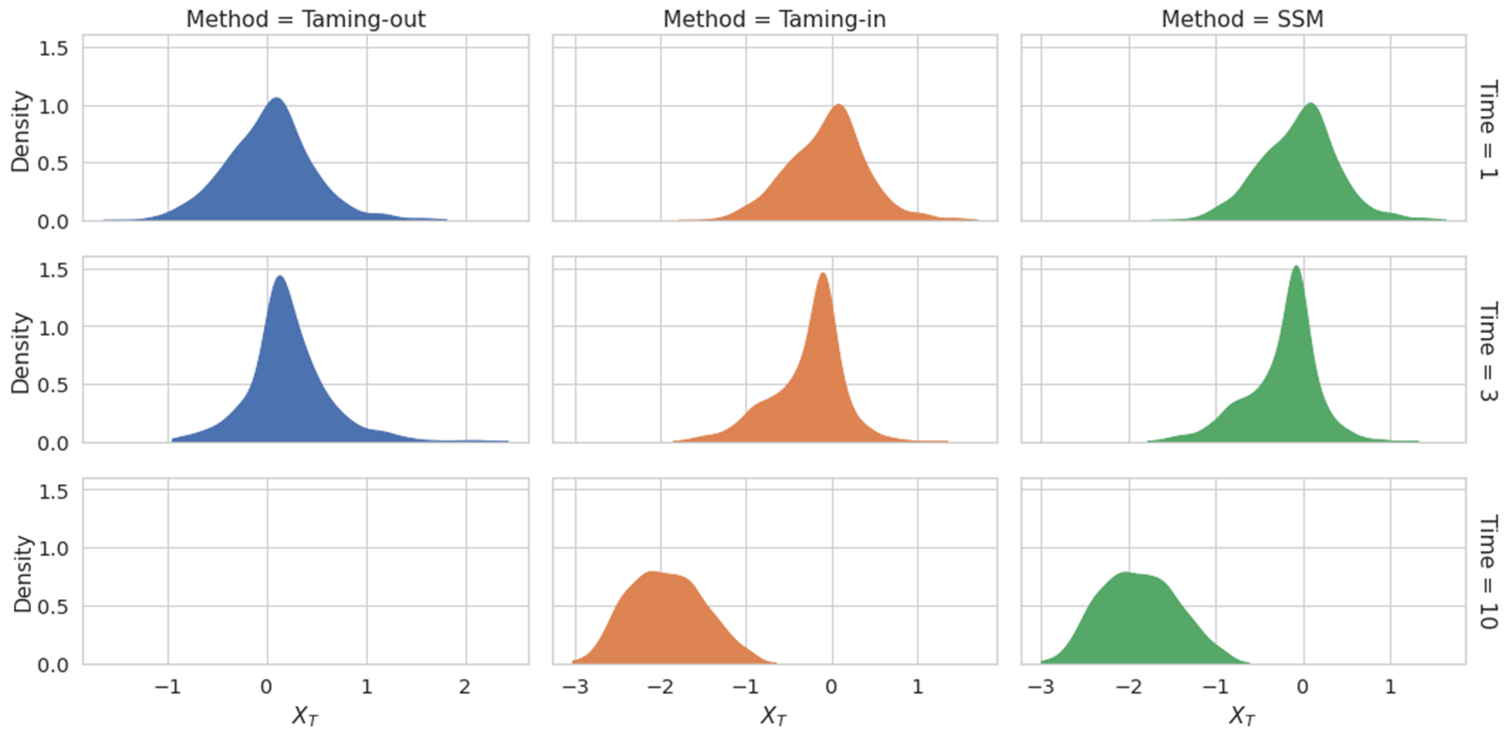
(a) Density with $X_{0}\sim\mathcal{N}(0,1)$

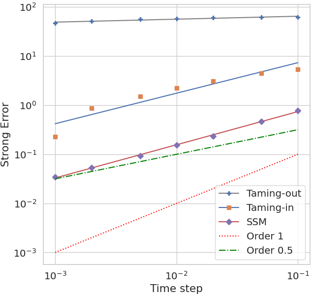
(b) Strong error (rMSE)

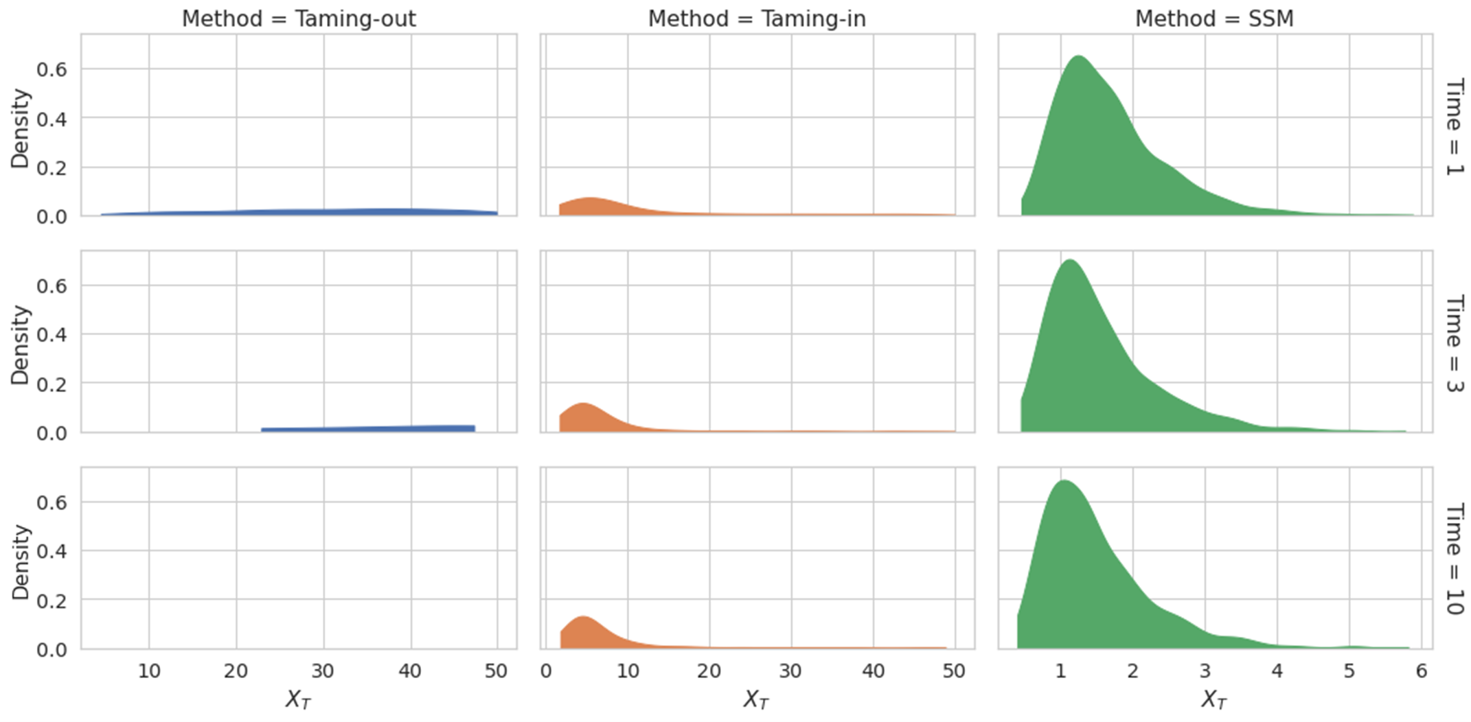
(c) Density with $X_{0}\sim B(50,0.5)$

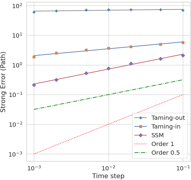
(d) Strong error (Path)

Figure 3.1: Simulation of the double-well model (3.2) with $N=1000$ particles. All schemes are initialized on the exact same samples. (a) and (c) show the density map for Taming-out (left), Taming-in (middle) and SSM (right) with $h=0.01$ at times $T\in\{1,3,10\}$ seen top-to-bottom and with different initial distribution. (b) Strong error (rMSE) of SSM and Taming with $X_{0}\sim\mathcal{N}(3,9)$ in log-scale. (d) Strong error (Path) of SSM and Taming with $X_{0}\sim\mathcal{N}(3,9)$ in log-scale.

The goal of this example is to simulate the interacting particle system associated to (3.2) up to $T=10$ using the three numerical methods available. Note that Theorem 2.7 does not apply here for the parameter choice in (3.2). Figure 3.1 (a) and (c) show the evolution of the density map at $T\in\{1,3,10\}$. In (a) with $X_{0}\sim\mathcal{N}(0,1)$, all three methods yield similar results, but (c) shows that with $X_{0}\sim B(50,0.5)$, Taming-out (blue, left) and Taming-in fail to produce acceptable results, while the SSM produces the expected results.

Figure 3.1 (b) shows the strong convergence of the methods, Taming-out failed to converge. Taming-in and the SSM converge under all time step choices (all satisfying (2.14)) and nearly attain the $1/2$ strong error rate, the error of SSM is one order of magnitude smaller than the error of Taming-in. Figure 3.1 (d) shows the path type strong convergence of both methods, and we observe that Taming-out and Taming-in failed to converge or at least converge with a very low rate. The SSM converges under all time step choices but the errors are one order of magnitude greater than the standard strong error.

As mentioned earlier, we do not have any theoretical support for the convergence of the taming methods. This example shows that a convergence proof for Taming-in might be feasible, possibly, under the caveat of an additional condition on the distribution/support of the initial condition – this was fully unforeseen. These results for Taming-out are discouraging, nonetheless, under strong dissipativity Taming-out seems stable (see next example).

3.2 Example: Approximating the invariant distribution

This example aims to illustrate the long-time simulation for the purpose of approximating the invariant distribution of the system

$$\mathrm{d}X_{t} =\big{(}v(X_{t},\mu_{t}^{X})-X_{t}\big{)}\mathrm{d}t+\tfrac{1}{4}(1-X_{t}^{2})\mathrm{d}W_{t},\leavevmode\nobreak\ v(x,\mu)=-x^{3}+\int_{\mathbb{R}}-\big{(}x-y\big{)}^{3}\mu(\mathrm{d}y).$$ (3.3)

The corresponding Fokker-Planck equation is $\partial_{t}\rho=\nabla[\leavevmode\nobreak\ \nabla\frac{\rho}{32}|1-x^{2}|^{2}+\rho\nabla V+\rho\nabla W*\rho]$ with $W=\frac{1}{4}|x|^{4}$, $V=\frac{1}{4}|x|^{4}+\frac{1}{2}|x|^{2}$, and $\rho$ is the corresponding density map. We know that there is a unique invariant distribution, see Theorem 2.7. Here, the cluster state is $x=0$.

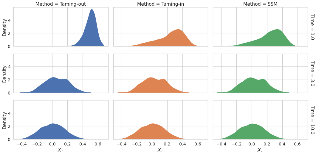
(a) Density with $X_{0}\sim\mathcal{N}(2,16)$

(b) Strong error

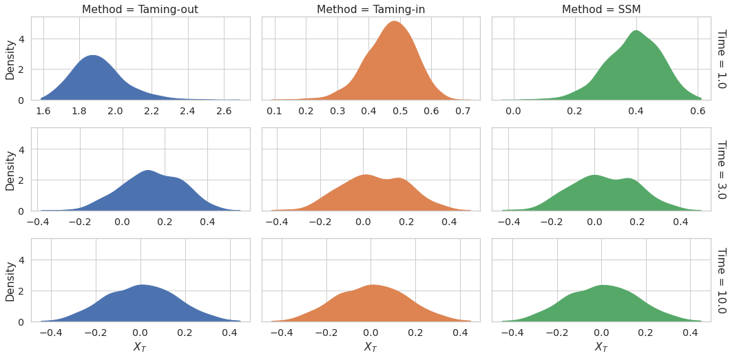
(c) Density with $X_{0}\sim U(4,12)$

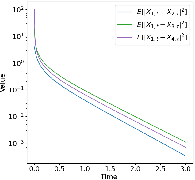
(d) Expected particle distance (SSM)

Figure 3.2: Approximation of the invariant distribution of (3.3) with $N=1000$ particles. The simulated Brownian motion paths and initial distribution are the same for all schemes. (a) and (c) show the distribution for Taming-out (left), Taming-in (middle) and SSM (right) with $h=0.01$ at times $T\in\{1,3,10\}$ seen top-to-bottom and with different initial distribution; $x$- and $y$-scales are fixed. (b) Strong error (rMSE) of SSM and Taming with $X_{0}\sim\mathcal{N}(2,16)$. (d) Expected distance (in log-scale) between particles under different initial distribution with $h=10^{-3}$ for the SSM.

Figure 3.2 (a) and (c) show the evolution of the particle distribution under different initial conditions. All three methods produce similar outputs at $T\in\{3,\leavevmode\nobreak\ 10\}$, with Taming-out taking longer to contract and to converge than the other methods under $X_{0}\sim\mathcal{N}(2,16)$ in (a) and $X_{0}\sim U(4,12)$ in (c). The similar results obtained at $T\in\{3,10\}$ are due to the fact that the model (3.3) has an invariant distribution and the initial distribution is compactly supported around the cluster state $x=0$.

Figure 3.2 (b) illustrates the strong convergence of the three methods: they all converge and the rates are of order close to $1/2$, the SSM outperforms the other two methods by $1$ to $2$ orders of magnitude. Figure 3.2 (d) depicts the expected exponential decay rate for the SSM under different initial conditions of Theorem 2.7: $X_{1,0}\sim\mathcal{N}(0,1)$, $X_{2,0}\sim U(-3,3)$, $X_{3,0}\sim\mathcal{N}(2,16)$, $X_{4,0}\sim\mathcal{N}(2,100)$ (same Brownian motion samples).

3.3 Example: Kinetic 2d Van der Pol oscillator and periodic phase-space

We consider a two-dimensional Van der Pol (VdP) oscillator model with added super-linearity terms. The VdP model was proposed to describe stable oscillation [45, Section 4.2 and 4.3] and for a system of many coupled oscillators in the presence of noise the limit model is a MV-SDE [2]. Here, we build a two-dimensional VdP-type model with mean-field components and super-diffusivity that features a periodicity of phase-space to show that the SSM preserves the theoretical periodic behaviour in simulation scenarios – see [16, Section 7.3].

Set $x=(x_{1},x_{2})\in\mathbb{R}^{2}$ and define the functions $f,u,b,\sigma$ as

$$f(x)=-x|x|^{2},\leavevmode\nobreak\ u(x)=\left[\begin{array}[]{c}-\frac{1}{3}x_{1}^{3}\\ 0\end{array}\right],\leavevmode\nobreak\ b(x)=\left[\begin{array}[]{c}x_{1}-x_{2}\\ x_{1}\end{array}\right],\leavevmode\nobreak\ \sigma(x)=\left[\begin{array}[]{ccc}1+1/4\leavevmode\nobreak\ x_{1}^{2}&0\\ 0&0\end{array}\right],$$ (3.10)

where $f$ satisfies $(\mathbf{A}^{f})$.

(a) $N=50$

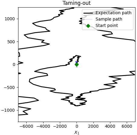
(b) $N=200$

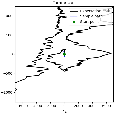
(c) $N=500$

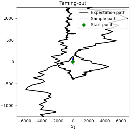
(d) $N=1000$

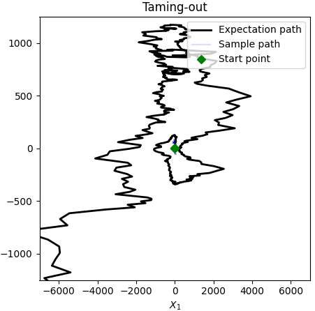
(e) $N=2000$

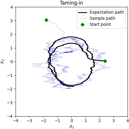
(f) $N=50$

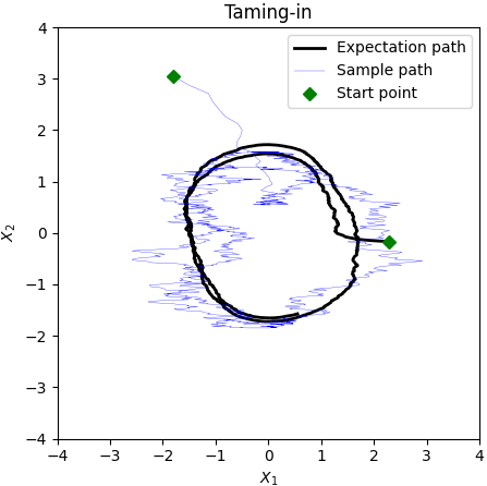
(g) $N=200$

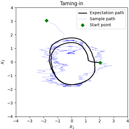
(h) $N=500$

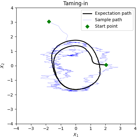
(i) $N=1000$

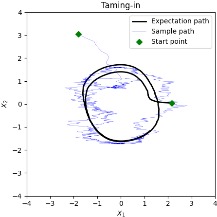
(j) $N=2000$

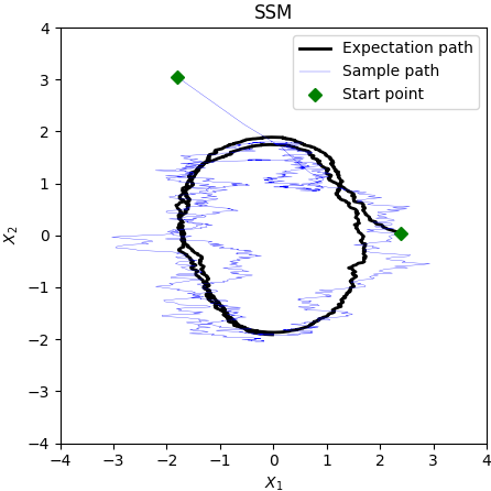
(k) $N=50$

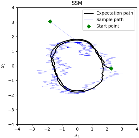
(l) $N=200$

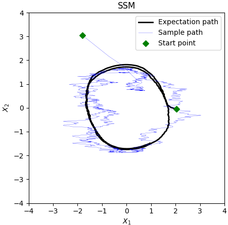
(m) $N=500$

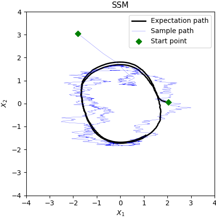
(n) $N=1000$

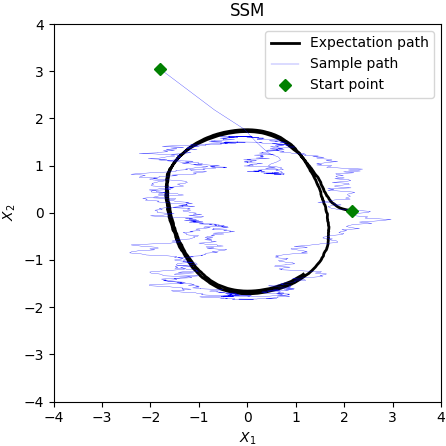
(o) $N=2000$

Figure 3.3: Simulation of the Vdp model (3.10) with a different number of particles and $h=10^{-2}$, $T=12$, $X_{1,0}\sim\mathcal{N}(2,16),X_{2,0}\sim\mathcal{N}(0,16)$. (a)(b)(c)(d)(e) are phase portraits of the Taming-out method with different choices of $N$. (f)(g)(h)(i)(j) are phase portraits of the Taming-in method with different choices of $N$. (k)(l)(m)(n)(o) are phase portraits of the SSM with different choices of $N$.

Figure 3.3 (a)-(o) show the system’s phase-space portraits (i.e., the parametric plot of $t\mapsto(X_{1,t},X_{2,t})$ and $t\mapsto(\mathbb{E}[X_{1,t}],\mathbb{E}[X_{2,t}])$) for the three methods with different choices of $N$.

In the first row of Figure 3.3, (a)-(e) shows the result of the Taming-out method, the system fails to converge for $N>50$. The second row and third row of Figure 3.3 show the result of Taming-in and the SSM, both methods converge and the trajectory becomes smoother as more particles are taken. However, there is a big difference on the expectation trajectories of the SSM and Taming in, the expectation trajectories of the SSM do not cross themselves while the expectation trajectories of Taming-in always cross themselves, which is not expected since the slope fields of the VdP model are smooth and do not admit the cross. Moreover, comparing the first few steps in the sample paths, the particles generated by the SSM concentrate to the expectation path within two steps while the one generated by Taming-in takes about 10 steps. This is because the SSM preserves the super-linear power from the convolution kernel while the Taming-in turns this power to an asymptotic linear one. Thus, the SSM preserves more geometric properties than the taming method even though the approximation obtained via taming may not blow up.

3.4 Example: Super-linear growth of measure components in diffusion

This example aims to illustrate the effect of two additional types of measure-nonlinearities included in the diffusion term; Case 1 corresponds to a convolution term in the diffusion and Case 2 is a variance-type term (which is beyond the scope of the paper). Note that the assumptions of the wellposedness result are not satisfied as the estimate (2.1) does not hold (but could readily be achieved by slightly modifying the constants of the coefficients), which indicates that this bound is not sharp. We consider

$$\mathrm{d}X_{t} =\big{(}v(X_{t},\mu_{t}^{X})+X_{t}\big{)}\mathrm{d}t+\big{(}X_{t}+\tfrac{1}{4}X_{t}^{2}+f_{\sigma}(X_{t},\mu_{t}^{X})\big{)}\mathrm{d}W_{t},\leavevmode\nobreak\$$ (3.11)

$$\textit{with}\leavevmode\nobreak\ v(x,\mu) =-\tfrac{1}{4}x^{3}+\int_{\mathbb{R}}-\big{(}x-y\big{)}^{3}\mu(\mathrm{d}y),\leavevmode\nobreak\ f_{\sigma}(x,\mu)=\begin{cases}\int_{\mathbb{R}}\big{(}x-y\big{)}^{2}\mu(\mathrm{d}y),\leavevmode\nobreak\ \textit{Case 1,}\\ \int_{\mathbb{R}}\int_{\mathbb{R}}\big{(}y-z\big{)}^{2}\mu(\mathrm{d}y)\mu(\mathrm{d}z),\leavevmode\nobreak\ \textit{Case 2.}\end{cases}$$

For Case 1, we have a nonlinear convolution kernel $f_{\sigma}(x)=x^{2}$ for all $x\in\mathbb{R}$. Figure 3.4, in particular, subplots (a)-(c), illustrates that the SSM converges, in a pointwise sense, with strong order $1/2$ and recovers reasonable density estimates for different choices of the initial distribution. Similar behaviour is not observed for different taming approaches which fail to recover the anticipated strong convergence order of $1/2$ and we observe that taming schemes do not capture the density of the solution well for high-variance initial data. We conducted an analogous test with $v(x,\mu)=-x^{3}/4$ in (d), i.e., we removed the convolution term in the drift, and our experiments failed, in the sense that the approximate solutions computed by the SSM did not converge. This supports our theoretical results that a suitable drift compensation for the nonlinear measure component appearing in the diffusion is indeed needed.

Case 2 corresponds to an example, where the convolution term is again integrated, i.e., resembles a variance-type term. We are not aware of an existing result that yields wellposedness of the underlying MV-SDE including such a term (even without the nonlinear convolution terms). Further, it is not clear which assumptions would be required for a numerical scheme to converge in a strong sense. The expected strong convergence order is observed for the SSM in (e), but no taming approach appears to be a reasonable alternative. We additionally conducted a numerical experiment for Case 2 with $v(x,\mu)=-x^{3}/4$, in order to investigate if the variance-type term requires a compensation term (similar to changed Case 1). We also observed that no time-stepping scheme (i.e., taming and SSM) seemed to converge (the result is similar to (d) and we do not present here), which again indicates that the drift’s convolution term can also help to control variance-type terms in the diffusion.

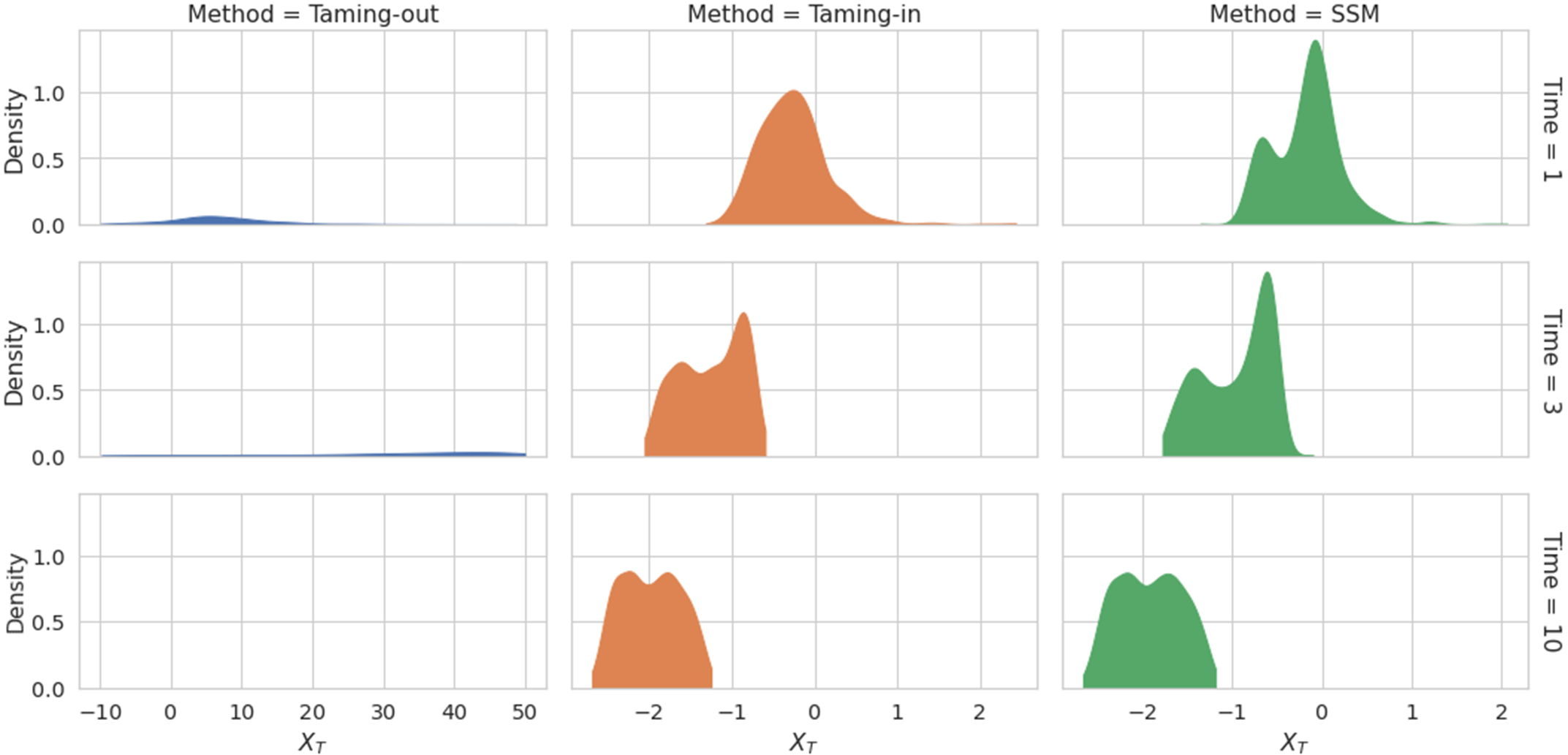
(a) Case 1-Density with $X_{0}\sim\mathcal{N}(0,1)$

(b) Case 1-Strong error

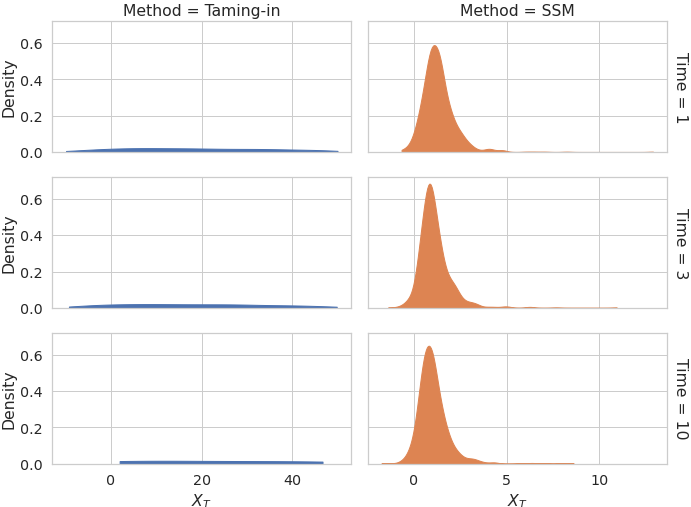
(c) Case 1-Density with $X_{0}\sim B(50,0.5)$

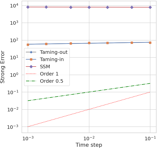
(d) Changed Case 1-Strong error

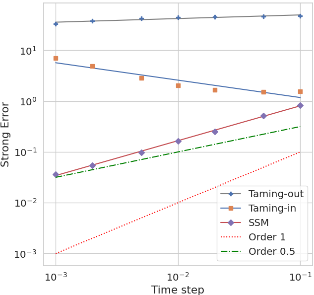
(e) Case 2-Strong error

Figure 3.4: Approximation of (3.11) with $N=1000$ particles. The simulated Brownian motion sample paths and initial distribution are the same for all schemes. (a) and (c) show the distribution for Taming-out (left), Taming-in (middle) and SSM (right) with $h=0.01$ at times $T\in\{1,3,10\}$ seen top-to-bottom and with different initial distribution; $x$- and $y$-scales are fixed. (b), (d) and (e) show the strong error (rMSE) of SSM and Taming with $X_{0}\sim\mathcal{N}(1,1)$ for different cases. The changed Case 1 in (d) is Case 1 with $v(x,\mu)=-x^{3}/4.$

3.5 Example: Propagation of Chaos rate across dimensions

In this example, we estimate the PoC rate depending on the dimension and compare the findings to the theoretical upper bounds established in Theorem 2.9. For equation (1.1)-(1.2) we make the following choices: Let $d\geq 2$, $x=(x_{1},\ldots,x_{d})\in\mathbb{R}^{d}$, the initial condition $X_{0}$ is a vector distributed according to $d$-independent $\mathcal{N}(1,1)$-random variables, and

$$f(x) =-x|x|^{2},\quad u(x)=-\frac{1}{3}\left[\begin{array}[]{cccc}x_{1}^{3},x_{2}^{3},\cdots,x_{d}^{3}\end{array}\right]^{\intercal},\quad b(t,x,\mu)=x,\quad$$ (3.13)

$$\overline{\sigma}(x) =\left[\begin{array}[]{cccc}x_{1}+1/4\leavevmode\nobreak\ x_{1}^{2}&x_{2}&\cdots&x_{d}\\ x_{1}&x_{2}+1/4\leavevmode\nobreak\ x_{2}^{2}&\cdots&x_{d}\\ \cdots&\cdots&\cdots&\cdots\\ x_{1}&x_{2}&\cdots&x_{d}+1/4\leavevmode\nobreak\ x_{d}^{2}\\ \end{array}\right].$$ (3.18)

This is a toy model with a high-dimensional fully coupled convolution kernel and super-linear diffusion term. We observe in Figure 3.5 a strong PoC rate, estimated via (3.1), of order of roughly $1/2$ across dimension $d$. By the ordinary least squares linear regression, for dimension $d\in\{2,3,4,6,10\}$, the corresponding slopes are $\{\textrm{slopes}_{d}\}_{d}=\{-0.55,-0.57,-0.5,-0.50,-0.49\}$ and the corresponding $R$-square measure is $\{R^{2}_{d}\}_{d}=\{0.81,0.75,0.92,0.91,0.98\}$.

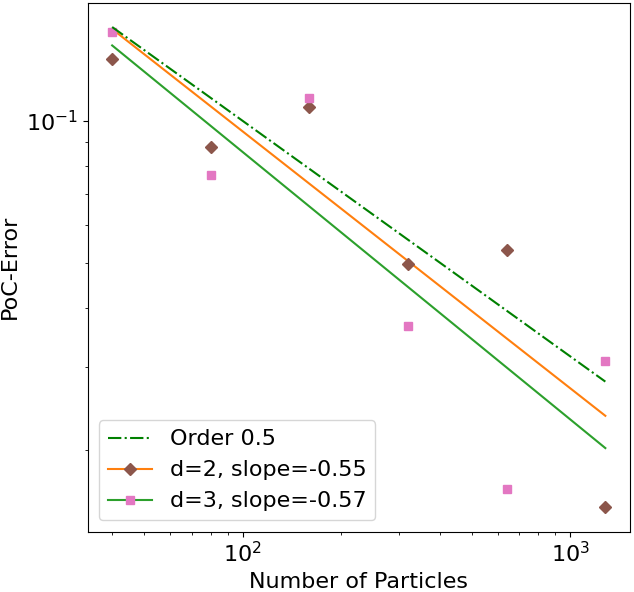
(a) PoC rates for $d\in\{2,3\}$

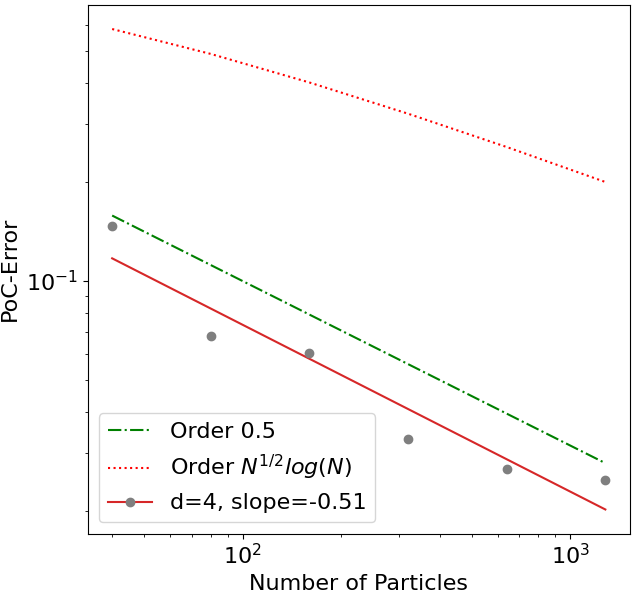
(b) PoC rates for $d=4$

(c) PoC rates for $d\in\{6,10\}$

Figure 3.5: Estimation of PoC rate for equation (1.1)-(1.2) under (3.18) using SSM (2.11)-(2.13) with fixed stepsize $h=10^{-3}$, $T=1$ and number of particles $N\in\{40,80,160,320,640,1280,2560\}$. In all figures the reference rate $0.5$ and the upper bound rate from Theorem 2.9 are displayed.

These findings are inline with those obtained in the one-dimensional example of [60, Example 4.1]. Theorem 2.9 establishes a strong convergence rate (in terms of number of particles in a pathwise sense) of order $1/4$ for dimensions $d<4$ only and these results are smaller than the upper bounds of PoC in Theorem 2.9 – this highlights a gap in the literature to be explored in future research. For perspective, at a theoretical level the rate $1/2$ in $N$ is not new under stronger assumptions. This was obtained in [27, Lemma 5.1] or [65] when the drift and diffusion coefficients are assumed to satisfy strong regularity assumptions. Also in [56] for linear type MV-SDEs featuring diffusions $\mathbb{R}^{d}\ni x\mapsto\overline{\sigma}(x)$ and drifts with structure of the type $\mathbb{R}^{d}\ni x\mapsto\int_{\mathbb{R}^{d}}b(x,y)\mu(\mathrm{d}y)$, and requiring that $b,\overline{\sigma}$ are uniformly Lipschitz, the convergence rate $1/2$ in the number of particles is obtained; also in [28].

3.6 Discussion

We discuss the advantages of the SSM compared with the taming methods. The SSM converges under all cases, while the two types of taming failed to converge in some cases. The SSM requires an implicit solver for the convolution kernel but the running time of the SSM compared to the taming methods is only 2 to 3 times longer. From the numerical examples, we see that:

1. The two types of strong errors of the SSM are of order 0.5 and consistently outperform that of the proposed taming schemes. In fact, the taming methods are not even expected to converge, however, under a mild initial condition, it is hard to observe the divergence. In the tests with high variance initial distributions, the taming methods diverge while SSM converges consistently. The SSM preserves convergence for larger time steps $h$ (via comparative lower errors) and is also suitable for long-time simulation.

2. The SSM preserves important geometric properties (the concentration speed of the particles is fast, the expected trajectory coincides with the vector field result), while the taming methods appear to fail to capture these crucial properties.

3. We applied the SSM to examples, where the diffusion also involves certain nonlinear measure terms. As long as a suitable monotonicity condition is satisfied the SSM yields promising results.

4. We perform a PoC rate test across dimensions with non-trivial convolution kernel. The rate which we observe numerically is better than the one suggested by the PoC results.

4 Proof of the main results

4.1 Proof of Theorem 2.5 : Wellposedness and moment stability

Proof of Theorem 2.5.

The existence and uniqueness follow from modifications of the methodologies used in [3, Theorem 3.5].

Wellposedness. The proof for existence and uniqueness follows along the same lines as the arguments presented in [3, Theorem 3.5]. We repeat here the main steps for convenience. As opposed to more classical approaches, the fixed point argument is carried out over a suitable function space, see [9], instead of a measure space.

To be precise, one considers the function space $\Lambda_{[0,T],q}$, for $q$ as in Assumption 2.1, defined as the space of continuous functions $\boldsymbol{g}:[0,T]\times\mathbb{R}^{d}\to\mathbb{R}^{d}\times\mathbb{R}^{d\times l}$, $\boldsymbol{g}(t,x)=(g_{1}(t,x),g_{2}(t,x))$ with $g_{1}:[0,T]\times\mathbb{R}^{d}\to\mathbb{R}^{d}$ and $g_{2}:[0,T]\times\mathbb{R}^{d}\to\mathbb{R}^{d\times l}$, satisfying

$$\|\boldsymbol{g}\|_{[0,T],q}:=\sup_{t\in[0,T]}\bigg{(}\sup_{x\in\mathbb{R}^{d}}\frac{|\boldsymbol{g}(t,x)|}{1+|x|^{q+1}}\bigg{)}<\infty,$$ (4.1)

and there exists a constant $L_{1}\geq 0$ such that (with $m$ as in Assumption 2.1)

$$\left\langle x-y,g_{1}(t,x)-g_{1}(t,y)\right\rangle+2(m-1)|g_{2}(t,x)-g_{2}(t,y)|^{2} \leq L_{1}|x-y|^{2},$$ (4.2)

for all $t\in[0,T]$, $x,y\in\mathbb{R}^{d}$. In particular, this implies that there exists a constant $L_{2}\geq 0$ such that

$$\left\langle x,g_{1}(t,x)\right\rangle+2(m-1)|g_{2}(t,x)|^{2}\leq L_{2}(1+|\boldsymbol{g}(t,0)|^{2}+|x|^{2}).$$

For some $K>0$ (chosen below), and a small enough terminal time $T_{0}$, we define now

$$E:=\{\boldsymbol{g}\in\Lambda_{[0,T_{0}],q}:\|\boldsymbol{g}\|_{[0,T_{0}],q}\leq K\}.$$

We claim that there exist choices for $T_{0}$ and $K$ such that $\Gamma:E\to E$ defined by

$$\Gamma[\boldsymbol{g}](t,x)=(\Gamma[\boldsymbol{g}]_{1}(t,x),\Gamma[\boldsymbol{g}]_{2}(t,x)):=(f\ast\mu_{t}^{\boldsymbol{g}}(x),f_{\sigma}\ast\mu_{t}^{\boldsymbol{g}}(x)),$$

forms a contraction. Here, $\mu^{\boldsymbol{g}}$ is the law of the solution to the MV-SDE

$$\mathrm{d}X^{\boldsymbol{g}}_{t} =\big{(}v^{\boldsymbol{g}}(t,X^{\boldsymbol{g}}_{t},\mu^{\boldsymbol{g}}_{t})+b(t,X^{\boldsymbol{g}}_{t},\mu^{\boldsymbol{g}}_{t})\big{)}\mathrm{d}t+\sigma^{\boldsymbol{g}}(t,X^{\boldsymbol{g}}_{t},\mu_{t}^{\boldsymbol{g}})\mathrm{d}W_{t},\quad X^{\boldsymbol{g}}_{0}=X_{0}\in L^{m}(\mathbb{R}^{d})$$ (4.3)

$$v^{\boldsymbol{g}}(t,x,\mu) =g_{1}(t,x)+u(x,\mu),\quad\sigma^{\boldsymbol{g}}(t,x,\mu)=\sigma(t,x,\mu)+g_{2}(t,x).$$ (4.4)

The existence of a unique strong solution to $(X^{\boldsymbol{g}}_{t})_{t\in[0,T]}$ satisfying $\sup_{t\in[0,T]}\mathbb{E}[|X_{t}^{g}|^{m}]\leq C$ for some constant $C>0$, is shown in [11, 49].

We first show that there exist $0<T_{0}<T$ and $K$ such that $\Gamma$ indeed maps $E$ onto itself. Let $\boldsymbol{g}\in E$. First, we observe that for all $x,y\in\mathbb{R}^{d}$, $t\in[0,T_{0}]$

$$\left\langle x-y,\Gamma[\boldsymbol{g}]_{1}(t,x)-\Gamma[\boldsymbol{g}]_{1}(t,y)\right\rangle+2(m-1)|\Gamma[\boldsymbol{g}]_{2}(t,x)-\Gamma[\boldsymbol{g}]_{2}(t,y)|^{2}$$

$$\leq\int_{\mathbb{R}^{d}}\left(\left\langle x-y,f(x-u)-f(y-u)\right\rangle+2(m-1)|f_{\sigma}(x-u)-f_{\sigma}(y-u)|^{2}\right)\mu_{t}^{\boldsymbol{g}}(\mathrm{d}u)\leq L_{1}|x-y|^{2}.$$

Further, we derive, using that $(X^{\boldsymbol{g}}_{t})_{t\in[0,T]}$ has finite moments of order $m>2(q+1)$ that there exist constants $C>0$ and $C(q,\mathbb{E}[|X_{0}|^{q+1}])>0$ (depending on the moment bounds of the initial data, $q$, and the model parameters) such that

$$\|\Gamma[\boldsymbol{g}] \|_{[0,T_{0}],q}\leq\sup_{t\in[0,T_{0}]}\bigg{(}\sup_{x\in\mathbb{R}^{d}}\frac{|(f\ast\mu_{t}^{g})(x)|+|(f_{\sigma}\ast\mu_{t}^{g})(x)|}{1+|x|^{q+1}}\bigg{)}\leq C\Big{(}1+\sup_{t\in[0,T_{0}]}\mathbb{E}\big{[}|X^{\boldsymbol{g}}_{t}|^{q+1}\big{]}\Big{)}$$ (4.5)

$${\color[rgb]{0,0,0}\leq C+Ce^{CT_{0}}\bigg{(}\mathbb{E}[|X_{0}|^{q+1}]+\int_{0}^{T_{0}}\leavevmode\nobreak\ \Big{(}|b(s,0,\delta_{0})|^{q+1}+|\boldsymbol{g}_{1}(s,0)|^{q+1}+|\boldsymbol{g}_{2}(s,0)|^{q+1}+|u(0,\delta_{0})|^{q+1}+|\sigma(s,0,\delta_{0})|^{q+1}\Big{)}\mathrm{d}s\bigg{)}}$$

$${\color[rgb]{0,0,0}\leq C+Ce^{CT_{0}}\bigg{(}\mathbb{E}[|X_{0}|^{q+1}]+T_{0}\|{\boldsymbol{g}}\|_{[0,T_{0}],q}^{q+1}+\int_{0}^{T_{0}}\leavevmode\nobreak\ \Big{(}|b(s,0,\delta_{0})|^{q+1}+|u(0,\delta_{0})|^{q+1}+|\sigma(s,0,\delta_{0})|^{q+1}\Big{)}\mathrm{d}s\bigg{)}}$$

$${\color[rgb]{0,0,0}\leq C+Ce^{CT_{0}}\bigg{(}\mathbb{E}[|X_{0}|^{q+1}]+T_{0}K^{q+1}+\int_{0}^{T_{0}}\leavevmode\nobreak\ \Big{(}|b(s,0,\delta_{0})|^{q+1}+|u(0,\delta_{0})|^{q+1}+|\sigma(s,0,\delta_{0})|^{q+1}\Big{)}\mathrm{d}s\bigg{)}\leq K,}$$

for a sufficiently small $T_{0}>0$ and the choice $K=2C(1+e^{CT}\mathbb{E}[|X_{0}|^{q+1}])$. It remains to show that the map $\Gamma:E\to E$ forms a contraction, i.e., for any $\boldsymbol{g}_{1}=(g_{1,1},g_{1,2}),\boldsymbol{g}_{2}=(g_{2,1},g_{2,2})\in E$, we have

$$\|\Gamma[\boldsymbol{g}_{1}]-\Gamma[\boldsymbol{g}_{2}]\|_{{[0,T_{0}],q}}\leq c\|\boldsymbol{g}_{1}-\boldsymbol{g}_{2}\|_{[0,T_{0}],q},$$

for $c\in(0,1)$ and a $T_{0}$ possibly even smaller than chosen above. An application of Itô’s formula shows for $t\in[0,T_{0}]$

$$\mathbb{E}[ |X^{\boldsymbol{g}_{1}}_{t}-X^{\boldsymbol{g}_{2}}_{t}|^{2}]\leq\mathbb{E}[|X^{\boldsymbol{g}_{1}}_{0}-X^{\boldsymbol{g}_{2}}_{0}|^{2}]+2\int_{0}^{t}\mathbb{E}\Big{[}\langle X^{{\boldsymbol{g}}_{1}}_{s}-X^{{\boldsymbol{g}}_{2}}_{s},v^{\boldsymbol{g}}(s,X^{{\boldsymbol{g}}_{1}}_{s},\mu_{s}^{{\boldsymbol{g}}_{1}})-v^{\boldsymbol{g}}(s,X^{{\boldsymbol{g}}_{2}}_{s},\mu_{s}^{{\boldsymbol{g}}_{2}})\rangle\Big{]}\mathrm{d}s$$

$$+2\int_{0}^{t}\mathbb{E}\Big{[}\langle X^{{\boldsymbol{g}}_{1}}_{s}-X^{{\boldsymbol{g}}_{2}}_{s},b(s,X^{{\boldsymbol{g}}_{1}}_{s},\mu_{s}^{{\boldsymbol{g}}_{1}})-b(s,X^{{\boldsymbol{g}}_{2}}_{s},\mu_{s}^{{\boldsymbol{g}}_{2}})\rangle\Big{]}\mathrm{d}s+\int_{0}^{t}\mathbb{E}\Big{[}\big{|}\sigma^{\boldsymbol{g}}(s,X^{{\boldsymbol{g}}_{1}}_{s},\mu_{s}^{{\boldsymbol{g}}_{1}})-\sigma^{\boldsymbol{g}}(s,X^{{\boldsymbol{g}}_{2}}_{s},\mu_{s}^{{\boldsymbol{g}}_{2}})\big{|}^{2}\Big{]}\mathrm{d}s$$

$$\leq\mathbb{E}[|X^{\boldsymbol{g}_{1}}_{0}-X^{\boldsymbol{g}_{2}}_{0}|^{2}]+C\int_{0}^{t}\mathbb{E}\Big{[}\big{|}X^{{\boldsymbol{g}}_{1}}_{s}-X^{{\boldsymbol{g}}_{2}}_{s}\big{|}^{2}\Big{]}\mathrm{d}s$$

$$\quad+2\int_{0}^{t}\mathbb{E}\Big{[}\langle X^{{\boldsymbol{g}}_{1}}_{s}-X^{{\boldsymbol{g}}_{2}}_{s},g_{1,1}(s,X^{{\boldsymbol{g}}_{1}}_{s})-g_{1,1}(s,X^{{\boldsymbol{g}}_{2}}_{s})\rangle\Big{]}+2\mathbb{E}\Big{[}\big{|}g_{1,2}(s,X^{{\boldsymbol{g}}_{1}}_{s})-g_{1,2}(s,X^{{\boldsymbol{g}}_{2}}_{s})\big{|}^{2}\Big{]}\mathrm{d}s$$

$$\quad+2\int_{0}^{t}\mathbb{E}\Big{[}\langle X^{{\boldsymbol{g}}_{1}}_{s}-X^{{\boldsymbol{g}}_{2}}_{s},g_{1,1}(s,X^{{\boldsymbol{g}}_{2}}_{s})-g_{2,1}(s,X^{{\boldsymbol{g}}_{2}}_{s})\rangle\Big{]}+2\mathbb{E}\Big{[}\big{|}g_{1,2}(s,X^{{\boldsymbol{g}}_{2}}_{s})-g_{2,2}(s,X^{{\boldsymbol{g}}_{2}}_{s})\big{|}^{2}\Big{]}\mathrm{d}s$$

$$\leq{\color[rgb]{0,0,0}\mathbb{E}[|X^{\boldsymbol{g}_{1}}_{0}-X^{\boldsymbol{g}_{2}}_{0}|^{2}]+C\int_{0}^{t}\mathbb{E}\Big{[}\big{|}X^{{\boldsymbol{g}}_{1}}_{s}-X^{{\boldsymbol{g}}_{2}}_{s}\big{|}^{2}\Big{]}\mathrm{d}s+4\int_{0}^{t}\mathbb{E}\Big{[}\big{|}g_{1,1}(s,X^{{\boldsymbol{g}}_{2}}_{s})-g_{2,1}(s,X^{{\boldsymbol{g}}_{2}}_{s})\big{|}^{2}+\big{|}g_{1,2}(s,X^{{\boldsymbol{g}}_{2}}_{s})-g_{2,2}(s,X^{{\boldsymbol{g}}_{2}}_{s})\big{|}^{2}\Big{]}\mathrm{d}s}$$

$$\leq{\color[rgb]{0,0,0}\mathbb{E}[|X^{\boldsymbol{g}_{1}}_{0}-X^{\boldsymbol{g}_{2}}_{0}|^{2}]+C\int_{0}^{t}\mathbb{E}\Big{[}\big{|}X^{{\boldsymbol{g}}_{1}}_{s}-X^{{\boldsymbol{g}}_{2}}_{s}\big{|}^{2}\Big{]}\mathrm{d}s+C\int_{0}^{t}\|\boldsymbol{g}_{1}-\boldsymbol{g}_{2}\|_{[0,T_{0}],q}^{2}\mathbb{E}[1+|X^{\boldsymbol{g}_{2}}_{s}|^{2q+2}]\mathrm{d}s},$$

where we used Young’s inequality in the last display. By Gronwall’s Lemma, we have

$$\sup_{t\in[0,T_{0}]}\mathbb{E}[ |X^{\boldsymbol{g}_{1}}_{t}-X^{\boldsymbol{g}_{2}}_{t}|^{2}]\leq CT_{0}e^{CT_{0}}\sup_{t\in[0,T_{0}]}\mathbb{E}[1+|X^{\boldsymbol{g}_{2}}_{t}|^{2q+2}]\|\boldsymbol{g}_{1}-\boldsymbol{g}_{2}\|_{[0,T_{0}],q}^{2}$$

From the result above, we have

$$\|\Gamma[\boldsymbol{g}_{1}]-\Gamma[\boldsymbol{g}_{2}] \|_{{[0,T_{0}],q}}\leq\sup_{t\in[0,T_{0}]}\bigg{(}\sup_{x\in\mathbb{R}^{d}}\frac{|(f\ast\mu_{t}^{\boldsymbol{g}_{1}})(x)-(f\ast\mu_{t}^{\boldsymbol{g}_{2}})(x)|+|(f_{\sigma}\ast\mu_{t}^{\boldsymbol{g}_{1}})(x)-(f_{\sigma}\ast\mu_{t}^{\boldsymbol{g}_{2}})(x)|}{1+|x|^{q+1}}\bigg{)}$$

$$\leq C\sup_{t\in[0,T_{0}]}\bigg{(}\sup_{x\in\mathbb{R}^{d}}\frac{\mathbb{E}\left[|X^{\boldsymbol{g}_{1}}_{t}-X^{\boldsymbol{g}_{2}}_{t}|(1+|x|^{q+1})\big{(}1+|X^{\boldsymbol{g}_{1}}_{t}|^{q}+|X^{\boldsymbol{g}_{2}}_{t}|^{q}\big{)}\right]}{1+|x|^{q+1}}\bigg{)}$$

$$\leq C\sup_{t\in[0,T_{0}]}\mathbb{E}\left[|X^{\boldsymbol{g}_{1}}_{t}-X^{\boldsymbol{g}_{2}}_{t}|\big{(}1+|X^{\boldsymbol{g}_{1}}_{t}|^{q}+|X^{\boldsymbol{g}_{2}}_{t}|^{q}\big{)}\right]$$

$$\leq C\Big{(}\sup_{t\in[0,T_{0}]}\mathbb{E}[|X^{\boldsymbol{g}_{1}}_{t}-X^{\boldsymbol{g}_{2}}_{t}|^{2}]\Big{)}^{1/2}\Big{(}\sup_{t\in[0,T_{0}]}\mathbb{E}\left[\left(1+|X^{\boldsymbol{g}_{1}}_{t}|^{q}+|X^{\boldsymbol{g}_{2}}_{t}|^{q}\right)^{2}\right]\Big{)}^{1/2}$$

$$\leq C\Big{(}e^{CT_{0}}\sqrt{T_{0}}\Big{)}\Big{(}\sup_{t\in[0,T_{0}]}\mathbb{E}[1+|X^{\boldsymbol{g}_{2}}_{t}|^{2q+2}]\Big{)}^{1/2}\Big{(}\sup_{t\in[0,T_{0}]}\mathbb{E}\left[\left(1+|X^{\boldsymbol{g}_{1}}_{t}|^{q}+|X^{\boldsymbol{g}_{2}}_{t}|^{q}\right)^{2}\right]\Big{)}^{1/2}\|\boldsymbol{g}_{1}-\boldsymbol{g}_{2}\|_{[0,T_{0}],q}$$

$$\leq C\Big{(}e^{CT_{0}}\sqrt{T_{0}}\Big{)}\leavevmode\nobreak\ {\color[rgb]{0,0,0}\Big{(}1+\sup_{t\in[0,T_{0}]}\mathbb{E}[|X^{\boldsymbol{g}_{1}}_{t}|^{2q+2}]+\sup_{t\in[0,T_{0}]}\mathbb{E}[|X^{\boldsymbol{g}_{2}}_{t}|^{2q+2}]\Big{)}}\|\boldsymbol{g}_{1}-\boldsymbol{g}_{2}\|_{{[0,T_{0}],q}},$$

where we used Young’s inequality in the last estimate. Performing similar calculations as above for the moments of $X^{\boldsymbol{g}_{1}}_{t}$ and $X^{\boldsymbol{g}_{2}}_{t}$, which by assumption exist up to order $m>2q+2$, allows to deduce that $T_{0}$ can indeed be chosen small enough such that $\Gamma$ maps $E$ onto $E$ and is a contraction operator. We conclude that the sequence $(\boldsymbol{g}^{n})_{n\geq 0}$ defined by $\boldsymbol{g}^{n+1}=\Gamma[\boldsymbol{g}^{n}]$, for $\boldsymbol{g}^{0}\in E$, is a Cauchy sequence belonging to $E$ and converges with respect to the $\|\cdot\|_{[0,T_{0}],q}$-norm to $\boldsymbol{g}=\Gamma[\boldsymbol{g}]$ satisfying (4.2). Thus, for all $t\in[0,T_{0}]$, we have

$$\boldsymbol{g}(t,X_{t}^{\boldsymbol{g}})=(f\ast\mu_{t}^{\boldsymbol{g}}(X_{t}^{\boldsymbol{g}}),f_{\sigma}\ast\mu_{t}^{\boldsymbol{g}}(X_{t}^{\boldsymbol{g}})).$$

Substituting this into (4.3), we obtain (1.1) and conclude $(X_{t})_{t\in[0,T_{0}]}$ with $\sup_{t\in[0,T_{0}]}\mathbb{E}\left[|X_{t}|^{m}\right]<\infty$.

Our challenge now is to find a solution over the whole interval $[0,T]$. From the above analysis, we observe that the implied constants (and therefore the choice of $T_{0}$) depend on the moments of $X_{0}$. Therefore, we are not immediately able to deduce the existence of a solution on $[0,T]$. We need to ensure that these constants do not explode.

Below, we show pointwise $p$-th moment estimates for $m\geq p>2$ (the case $p=2$ follows in a straightforward manner from the below arguments where one would use Lemma A.1 and Lemma A.2 instead of the additional symmetry property – we discuss this in more detail in Section 4.2 as we prove Theorem 2.7). From Itô’s formula, Assumption 2.1 and Remark 2.4, for all $t\in[0,T_{0}]$, we deduce

$$|X_{t}|^{p}\leq |X_{0}|^{p}+p\int_{0}^{t}|X_{s}|^{p-2}\langle X_{s},v(X_{s},\mu^{X}_{s})\rangle\mathrm{d}s+p\int_{0}^{t}|X_{s}|^{p-2}\langle X_{s},\overline{\sigma}(s,X_{s},\mu^{X}_{s})\mathrm{d}W_{s}\rangle$$ (4.6)

$$+p\int_{0}^{t}|X_{s}|^{p-2}\langle X_{s},b(s,X_{s},\mu^{X}_{s})\rangle\mathrm{d}s+p(p-1)\int_{0}^{t}|X_{s}|^{p-2}\Big{(}|\sigma(s,X_{s},\mu^{X}_{s})|^{2}+\int_{\mathbb{R}^{d}}|f_{\sigma}(X_{s}-y)|^{2}\mu^{X}_{s}(\mathrm{d}y)\Big{)}\mathrm{d}s$$

$$\leq |X_{0}|^{p}+C\int_{0}^{t}\Big{(}1+|X_{s}|^{p}+\big{(}W^{(2)}(\mu^{X}_{s},\delta_{0})\big{)}^{p}\Big{)}\mathrm{d}s+p\int_{0}^{t}|X_{s}|^{p-2}\langle X_{s},\overline{\sigma}(s,X_{s},\mu^{X}_{s})\mathrm{d}W_{s}\rangle$$

$$+p\int_{0}^{t}|X_{s}|^{p-2}\Big{(}\langle X_{s},\int_{\mathbb{R}^{d}}f(X_{s}-y)\mu^{X}_{s}(\mathrm{d}y)\rangle+(p-1)\int_{\mathbb{R}^{d}}|f_{\sigma}(X_{s}-y)|^{2}\mu^{X}_{s}(\mathrm{d}y)\Big{)}\mathrm{d}s.$$

Taking expectation on both sides, using Assumption 2.1, in particular $(\mathbf{A}^{f},\leavevmode\nobreak\ \mathbf{A}^{f_{\sigma}})$, and Remark 2.4, we derive

$$\mathbb{E} \big{[}|X_{t}|^{p}\big{]}\leq\mathbb{E}\big{[}|X_{0}|^{p}\big{]}+C\int_{0}^{t}(1+\mathbb{E}\big{[}|X_{s}|^{p}\big{]})\mathrm{d}s+\frac{p}{4}\int_{0}^{t}\int_{\mathbb{R}^{d}}\int_{\mathbb{R}^{d}}(|x|^{p-2}-|y|^{p-2})\langle x+y,f(x-y)\rangle\mu^{X}_{s}(\mathrm{d}x)\mu^{X}_{s}(\mathrm{d}y)\mathrm{d}s$$

$$\qquad+\frac{p}{2}\int_{0}^{t}\int_{\mathbb{R}^{d}}\int_{\mathbb{R}^{d}}|x|^{p-2}\big{(}\langle x-y,f(x-y)\rangle+2(p-1)|f_{\sigma}(x-y)|^{2}\big{)}\mu^{X}_{s}(\mathrm{d}x)\mu^{X}_{s}(\mathrm{d}y)\mathrm{d}s$$

$$\leq \mathbb{E}\big{[}|X_{0}|^{p}\big{]}+C\int_{0}^{t}\mathbb{E}\big{[}|X_{s}|^{p}\big{]}\mathrm{d}s+Ct.$$

Gronwall’s lemma yields the pointwise moment estimate,

$$\sup_{t\in[0,T_{0}]}\mathbb{E}\big{[}|X_{t}|^{\widetilde{m}}\big{]} \leq C\left(1+\mathbb{E}[|X_{0}|^{\widetilde{m}}]\right)e^{CT_{0}},\qquad\textrm{for any }\leavevmode\nobreak\ \widetilde{m}\in[2,m].$$ (4.7)

Since, we have established a-priori $L^{p}$-moment bounds, for $p\in[2,m]$, (which substitutes for [3, Proposition 3.13]), we can repeat the arguments from above to establish the existence of a solution to an arbitrary time interval $[0,T]$. To be more precise, we first show that we can choose constants $K_{1},T_{1}>0$ (independent of $T_{0}$) such that for $T_{0}+T_{1}\in[0,T]$ we have $\|\Gamma[\boldsymbol{g}]\|_{[T_{0},T_{0}+T_{1}],q}\leq K_{1}$, for $\|{\boldsymbol{g}}\|_{[T_{0},T_{0}+T_{1}],q}\leq K_{1}$. From Equation 4.5, we get

$$\|\Gamma[\boldsymbol{g}]\|_{[T_{0},T_{0}+T_{1}],q}$$

$$\leq C+Ce^{CT_{1}}\bigg{(}\sup_{t\in[0,T_{0}]}\mathbb{E}[|X_{t}|^{q+1}]+T_{1}\|{\boldsymbol{g}}\|_{[T_{0},T_{0}+T_{1}],q}^{q+1}+\int_{T_{0}}^{T_{0}+T_{1}}\leavevmode\nobreak\ \Big{(}|b(s,0,\delta_{0})|^{q+1}+|u(0,\delta_{0})|^{q+1}+|\sigma(s,0,\delta_{0})|^{q+1}\Big{)}\mathrm{d}s\bigg{)}$$

$$\leq C+Ce^{CT_{1}}\bigg{(}\sup_{t\in[0,T_{0}]}\mathbb{E}[|X_{t}|^{q+1}]+T_{1}K_{1}^{q+1}+\int_{T_{0}}^{T_{0}+T_{1}}\leavevmode\nobreak\ \Big{(}|b(s,0,\delta_{0})|^{q+1}+|u(0,\delta_{0})|^{q+1}+|\sigma(s,0,\delta_{0})|^{q+1}\Big{)}\mathrm{d}s\bigg{)}$$

$$\leq C+Ce^{CT_{1}}\bigg{(}e^{CT_{0}}\Big{(}1+\mathbb{E}[|X_{0}|^{q+1}]\Big{)}+T_{1}K_{1}^{q+1}+\int_{T_{0}}^{T_{0}+T_{1}}\leavevmode\nobreak\ \Big{(}|b(s,0,\delta_{0})|^{q+1}+|u(0,\delta_{0})|^{q+1}+|\sigma(s,0,\delta_{0})|^{q+1}\Big{)}\mathrm{d}s\bigg{)},$$

where we used (4.7) in the last inequality. Let now $K_{1}=2C(1+e^{CT}+e^{CT}\mathbb{E}[|X_{0}|^{q+1}])$. Then, we choose $T_{1}>0$ (independent of $T_{0}$) small enough such that for any $\|\boldsymbol{g}\|_{[T_{0},T_{0}+T_{1}],q}\leq K_{1}$, we have $\|\Gamma[\boldsymbol{g}]\|_{[T_{0},T_{0}+T_{1}],q}\leq K_{1}$. Similary as above, we can show that the map $\Gamma:E_{1}\to E_{1}$, where

$$E_{1}:=\{\boldsymbol{g}\in\Lambda_{[T_{0},T_{0}+T_{1}],q}:\|\boldsymbol{g}\|_{[T_{0},T_{0}+T_{1}],q}\leq K_{1}\},$$

forms a contraction (eventually choosing $T_{1}$ even smaller as above). The argument from above (choosing $K_{2}$ etc. as $K_{1}$) can be repeated to establish the existence of a solution on the time interval $[0,T]$.

∎

4.2 Proof of Theorem 2.7 : Exponential contraction and the ergodic property

Proof of Theorem 2.7.

We prove the statements by the order they were stated.

Proof of statement 1. Consider two solutions $X,Y$ of (1.1), driven by the same Brownian motion but with different initial conditions $X_{0}\sim\mu,Y_{0}\sim\nu$, $\mu,\nu\in\mathcal{P}_{\ell}(\mathbb{R}^{d}),\leavevmode\nobreak\ \ell>2q+2$. Let $\bar{X},\bar{Y}$ be independent copies of $X,Y$ respectively. By the wellposedness result these processes have finite moments up to order $\ell$. We now establish an exponential contraction statement: For all $t\in[0,\infty)$, using Itô’s formula and taking expectations, by Remark 2.4, we derive the following estimate

$$e^{-\rho_{1}t} \mathbb{E}\big{[}|X_{t}-Y_{t}|^{2}\big{]}=\mathbb{E}\big{[}|X_{0}-Y_{0}|^{2}\big{]}+2\int_{0}^{t}e^{-\rho_{1}s}\mathbb{E}\big{[}\langle X_{s}-Y_{s},v(X_{s},\mu^{X}_{s})-v(Y_{s},\mu^{Y}_{s})\rangle\big{]}\mathrm{d}s$$

$$\quad+\int_{0}^{t}e^{-\rho_{1}s}\mathbb{E}\big{[}2\langle X_{s}-Y_{s},b(s,X_{s},\mu^{X}_{s})-b(s,Y_{s},\mu^{Y}_{s})\rangle+|\overline{\sigma}(s,X_{s},\mu^{X}_{s})-\overline{\sigma}(s,Y_{s},\mu^{Y}_{s})|^{2}\big{]}\mathrm{d}s$$

$$\quad+\int_{0}^{t}(-\rho_{1})e^{-\rho_{1}s}\mathbb{E}\big{[}|X_{s}-Y_{s}|^{2}\big{]}\mathrm{d}s$$

$$\leq\mathbb{E}\big{[}|X_{0}-Y_{0}|^{2}\big{]}+\int_{0}^{t}e^{-\rho_{1}s}\mathbb{E}\big{[}2\langle X_{s}-Y_{s},b(s,X_{s},\mu^{X}_{s})-b(s,Y_{s},\mu^{Y}_{s})\rangle-\rho_{1}|X_{s}-Y_{s}|^{2}\big{]}\mathrm{d}s$$

$$\quad+2\int_{0}^{t}e^{-\rho_{1}s}\mathbb{E}\big{[}\langle X_{s}-Y_{s},f(X_{s}-\bar{X}_{s})-f(Y_{s}-\bar{Y}_{s})\rangle+|f_{\sigma}(X_{s}-\bar{X}_{s})-f_{\sigma}(Y_{s}-\bar{Y}_{s})|^{2}\big{]}\mathrm{d}s$$

$$\quad+2\int_{0}^{t}e^{-\rho_{1}s}\mathbb{E}\Big{[}\langle X_{s}-Y_{s},u(X_{s},\mu^{X}_{s})-u(Y_{s},\mu^{Y}_{s})\rangle+|\sigma(s,X_{s},\mu^{X}_{s})-\sigma(s,Y_{s},\mu^{Y}_{s})|^{2}\Big{]}\mathrm{d}s$$

$$\leq\mathbb{E}\big{[}|X_{0}-Y_{0}|^{2}\big{]}+\big{(}2L_{(b)}^{(2)}+2L_{(b)}^{(3)}+2L^{(1)}_{(u\sigma)}+2L^{(2)}_{(u\sigma)}-\rho_{1}\big{)}\int_{0}^{t}e^{-\rho_{1}s}\mathbb{E}\big{[}|X_{s}-Y_{s}|^{2}\big{]}\mathrm{d}s$$

$$\quad+2\int_{0}^{t}e^{-\rho_{1}s}\mathbb{E}\big{[}\langle X_{s}-Y_{s},f(X_{s}-\bar{X}_{s})-f(Y_{s}-\bar{Y}_{s})\rangle+|f_{\sigma}(X_{s}-\bar{X}_{s})-f_{\sigma}(Y_{s}-\bar{Y}_{s})|^{2}\big{]}\mathrm{d}s$$

$$\leq\mathbb{E}\big{[}|X_{0}-Y_{0}|^{2}\big{]}+\big{(}2L_{(b)}^{(2)}+2L_{(b)}^{(3)}+2L^{(1)}_{(u\sigma)}+2L^{(2)}_{(u\sigma)}+4L^{(1),+}_{(f)}-\rho_{1}\big{)}\int_{0}^{t}e^{-\rho_{1}s}\mathbb{E}\big{[}|X_{s}-Y_{s}|^{2}\big{]}\mathrm{d}s$$

$$=\mathbb{E}\big{[}|X_{0}-Y_{0}|^{2}\big{]},$$

where we used Remark 2.4 and the estimate

$$\mathbb{E}\big{[}\langle X_{s}-Y_{s},f(X_{s}-\bar{X}_{s})-f(Y_{s}-\bar{Y}_{s})\rangle+|f_{\sigma}(X_{s}-\bar{X}_{s})-f_{\sigma}(Y_{s}-\bar{Y}_{s})|^{2}\big{]}\leq 2L^{(1),+}_{(f)}\mathbb{E}\big{[}|X_{s}-Y_{s}|^{2}\big{]},$$

(see, Lemma A.2), and the definition of $\rho_{1}$ in Theorem 2.7. Using the properties of the Wasserstein metric, we obtain

$$\big{(}W^{(2)}(P^{*}_{0,t}\mu,P^{*}_{0,t}\nu)\big{)}^{2}=\big{(}W^{(2)}(\mu^{X}_{t},\mu^{Y}_{t})\big{)}^{2}\leq\mathbb{E}\big{[}|X_{t}-Y_{t}|^{2}\big{]} \leq\mathbb{E}\big{[}|X_{0}-Y_{0}|^{2}\big{]}e^{\rho_{1}t}$$

$$\leq e^{\rho_{1}t}\big{(}W^{(2)}(\mu,\nu)\big{)}^{2},$$ (4.8)

where in the last inequality we took the infimum on both sides over all couplings between $\mu$ and $\nu$. This concludes the proof of the first statement.

Proof of statement 2. Let the corresponding assumptions hold and let $X_{0}\sim\mu$, $\mu\in\mathcal{P}_{\ell}(\mathbb{R}^{d})$ with $2q+2<\ell\leq m$ be given. Applying similar calculations as in (4.6) for $e^{-\rho_{2,\ell}t}|X_{t}|^{\ell}$ (with $\rho_{2,\ell}\neq 0$), we deduce that there exists a constant $C>0$ depending on $\ell,\leavevmode\nobreak\ L^{(1)}_{(bu\sigma)}$ and $\sup_{t}|b(t,0,\delta_{0})|$ such that

$$e^{-\rho_{2,\ell}t}\mathbb{E}\big{[}|X_{t}|^{\ell}\big{]}\leq\mathbb{E}\big{[}|X_{0}|^{\ell}\big{]}+\int_{0}^{t}\ell e^{-\rho_{2,\ell}s}\mathbb{E}\big{[}|X_{s}|^{\ell-2}\big{(}\langle X_{s},f(X_{s}-\bar{X}_{s})\rangle+(\ell-1)|f_{\sigma}(X_{s}-\bar{X}_{s})|\big{)}\big{]}\mathrm{d}s$$

$$\qquad+\big{(}L^{(2)}_{(bu\sigma)}\ell+L^{(3)}_{(bu\sigma)}\ell-\rho_{2,\ell}\big{)}\int_{0}^{t}e^{-\rho_{2,\ell}s}\mathbb{E}\big{[}|X_{s}|^{\ell}\big{]}\mathrm{d}s+\ell\int_{0}^{t}e^{-\rho_{2,\ell}s}L^{(1)}_{(bu\sigma)}\mathbb{E}\big{[}|X_{s}|^{\ell-2}\big{]}\mathrm{d}s$$

$$\leq\mathbb{E}\big{[}|X_{0}|^{l}\big{]}+\frac{2(\ell L^{(1)}_{(bu\sigma)})^{\ell}}{\ell}\int_{0}^{t}e^{-\rho_{2,\ell}s}\mathrm{d}s+\Big{(}\ell(L^{(2)}_{(bu\sigma)}+L^{(3)}_{(bu\sigma)}+2L^{(1),+}_{(f)}+L^{(3)}_{(f)}/2)+\frac{\ell-2}{\ell}{}-\rho_{2,\ell}\Big{)}\int_{0}^{t}e^{-\rho_{2,\ell}s}\mathbb{E}\big{[}|X_{s}|^{\ell}\big{]}\mathrm{d}s$$

$$\leq\mathbb{E}\big{[}|X_{0}|^{l}\big{]}+\frac{C}{\rho_{2,\ell}}(1-e^{-\rho_{2,\ell}t}),$$

where we used Assumption 2.1 $(\mathbf{A}^{f},\leavevmode\nobreak\ \mathbf{A}^{f_{\sigma}})\leavevmode\nobreak\$, (2.4) and Young’s inequality for the last term in the first inequality. Similarly, for $\rho_{2,\ell}=0$, we have

$$\mathbb{E}\big{[}|X_{t}|^{\ell}\big{]}\leq\mathbb{E}\big{[}|X_{0}|^{\ell}\big{]}+Ct.$$

Using the properties of the Wasserstein metric we have

$$\big{(}W^{(\ell)}(P^{*}_{0,t}\mu,\delta_{0})\big{)}^{\ell} =\big{(}W^{(\ell)}(\mu^{X}_{t},\delta_{0})\big{)}^{\ell}\leq\mathbb{E}\big{[}|X_{t}|^{\ell}\big{]}$$

$$\leq\mathbb{E}\big{[}|X_{0}|^{\ell}\big{]}e^{\rho_{2,\ell}t}+\frac{C}{\rho_{2,\ell}}(e^{\rho_{2,\ell}t}-1)\mathbbm{1}_{\rho_{2,\ell}\neq 0}+Ct\mathbbm{1}_{\rho_{2,\ell}=0}$$

$$\leq e^{\rho_{2,\ell}t}\big{(}W^{(\ell)}(\mu,\delta_{0})\big{)}^{\ell}+\frac{C}{\rho_{2,\ell}}(e^{\rho_{2,\ell}t}-1)\mathbbm{1}_{\rho_{2,\ell}\neq 0}+Ct\mathbbm{1}_{\rho_{2,\ell}=0}.$$ (4.9)

Proof of statement 3. In the previous two statements we worked on the finite time interval $[0,T]$ and this statement extends the work to $[0,\infty)$. We also emphasize that the reason why we work with $\mathcal{P}_{2\ell-2}$ instead of $\mathcal{P}_{\ell}$ with $1+m/2\geq\ell>2q+2$ will become apparent later in the proof. Let $X_{0}\sim\mu_{0},Y_{0}\sim\nu_{0}$ with $\mu_{0},\nu_{0}\in\mathcal{P}_{2\ell-2}(\mathbb{R}^{d})$ be given.

From Theorem 2.5 and the flow property on $\mathcal{P}_{\ell}(\mathbb{R}^{d})$ of (1.1) described by the semigroup operator $(P^{*}_{s,t})$ (defined above Theorem 2.7), we extend $(\mu^{X}_{t})_{t\geq 0}$, $(\mu^{Y}_{t})_{t\geq 0}$ (e.g., via patching up solutions inductively over intervals $[nT,(n+1)T]$ for $n\in\mathbb{N}$). Further, since $\rho_{1}<0$, we have a contraction in (4.8) and hence $\lim_{t\rightarrow\infty}W^{(2)}(\mu^{X}_{t},\mu^{Y}_{t})=0$. By using $\rho_{2,2\ell-2}<0$, we have $\sup_{t\geq 0}W^{(2\ell-2)}(\mu^{X}_{t},\delta_{0})<\infty$, which guarantees that $\mu^{X}_{t}\in\mathcal{P}_{2\ell-2}(\mathbb{R}^{d})$ for all $t\geq 0$. The main proof follows via a shift-coupling argument and the properties shown so far under $\rho_{1},\rho_{2,2\ell-2}<0$, but with a critical additional element regarding establishing contraction and higher order moments for the candidate invariant measure so that the wellposedness result applies.

We start by showing that $(P^{*}_{0,t}\nu_{0})_{t\geq 0}$ is a Cauchy-sequence in $(\mathcal{P}_{2}(\mathbb{R}^{d}),W^{(2)})$, and use this result to show that $(P^{*}_{0,t}\nu_{0})_{t\geq 0}$ is also Cauchy-sequence in $(\mathcal{P}_{\ell}(\mathbb{R}^{d}),W^{({\ell})})$ for a given $\nu_{0}\in\mathcal{P}_{2\ell-2}(\mathbb{R}^{d})$. These arguments suffice to first find a candidate invariant distribution and then to characterize it as an ergodic limit (see below).

Using the $W^{(2)}$-contraction. Given $\nu_{0}\in\mathcal{P}_{2\ell-2}(\mathbb{R}^{d})$, from (2.5) with $\rho_{1}<0$, we have exponential contraction and hence for any $0\leq s<t<\infty$

$$W^{(2)}\big{(}P^{*}_{0,t}\nu_{0},P^{*}_{0,t+s}\nu_{0}\big{)}=W^{(2)}\big{(}P^{*}_{0,t}\nu_{0},P^{*}_{0,t}\big{(}P^{*}_{0,s}\nu_{0})\big{)}\leq e^{\rho_{1}t/2}W^{(2)}\big{(}\nu_{0},P^{*}_{0,s}\nu_{0}\big{)},$$

where we used the semigroup property that $P^{*}_{s,t}=P^{*}_{0,t-s}$ (since $b,\sigma$ are independent of $t$; see [69, 43, 52]).

The bounded orbit argument. From (2.6) with $\rho_{2,2\ell-2}<0$ and $m\geq 2\ell-2>4q+2$, we have via the triangle inequality

$$\sup_{t\geq 0} \big{(}W^{(2\ell-2)}\big{(}P^{*}_{0,t}\nu_{0},\nu_{0}\big{)}\big{)}^{2\ell-2}\leq C\Big{(}\big{(}W^{(2\ell-2)}\big{(}\nu_{0},\delta_{0}\big{)}\big{)}^{2\ell-2}+\sup_{t\geq 0}\big{(}W^{(2\ell-2)}\big{(}P^{*}_{0,t}\nu_{0},\delta_{0}\big{)}\big{)}^{2\ell-2}\Big{)}$$

$$\leq C\Big{(}\big{(}W^{(2\ell-2)}\big{(}\nu_{0},\delta_{0}\big{)}\big{)}^{2\ell-2}+\sup_{t\geq 0}\Big{(}e^{\rho_{2,2\ell-2}t}\big{(}W^{(2\ell-2)}\big{(}\nu_{0},\delta_{0}\big{)}\big{)}^{2\ell-2}\Big{)}+\sup_{t\geq 0}\frac{1}{\rho_{2,2\ell-2}}(e^{\rho_{2,2\ell-2}t}-1)\Big{)}$$

$$\leq C\Big{(}\big{(}W^{(2\ell-2)}\big{(}\nu_{0},\delta_{0}\big{)}\big{)}^{2\ell-2}-\tfrac{1}{\rho_{2,2\ell-2}}\Big{)}<\infty.$$ (4.10)

In other words, the orbit of $t\mapsto P^{*}_{0,t}\nu_{0}$ remains within a sufficiently large $W^{(2\ell-2)}$-ball, which also shows the finiteness of $\sup_{t\geq 0}W^{(2)}\big{(}P^{*}_{0,t}\nu_{0},\nu_{0}\big{)}$.

A $W^{(2)}$-Cauchy-sequence and the completeness argument. Combining the two previous elements we have

$$\lim_{s\to\infty}W^{(2)}\big{(}P^{*}_{0,t}\nu_{0},P^{*}_{0,t+s}\nu_{0}\big{)} =\lim_{s\to\infty}W^{(2)}\big{(}P^{*}_{0,t}\nu_{0},P^{*}_{0,t}(P^{*}_{0,s}\nu_{0})\big{)}$$

$$\leq e^{\rho_{1}t/2}\lim_{s\to\infty}W^{(2)}\big{(}\nu_{0},P^{*}_{0,s}\nu_{0}\big{)}\leq Ce^{\rho_{1}t/2}.$$

This shows the sequence to be Cauchy and since $(\mathcal{P}_{2}(\mathbb{R}^{d}),W^{(2)})$ is complete, there exists a limiting measure $\bar{\mu}\in\mathcal{P}_{2}(\mathbb{R}^{d})$ to the sequence, i.e., we have

$$\lim_{t\to\infty}W^{(2)}(P^{*}_{0,t}\nu_{0},\bar{\mu})=0.$$

The candidate invariant measure $\bar{\mu}$ has sufficiently high moments. The current issue with $\bar{\mu}\in\mathcal{P}_{2}({\mathbb{R}^{d}})$ is that we cannot guarantee, via Theorem 2.5, that $P^{*}_{0,t}\bar{\mu}$ has meaning (although we have convergence in $\mathcal{P}_{2}(\mathbb{R}^{d})$). Thus, we need to show that $(P^{*}_{0,t}\nu_{0})_{t\geq 0}$ also has the Cauchy-sequence property in $(\mathcal{P}_{\ell}(\mathbb{R}^{d}),W^{({\ell})})$ so that $\bar{\mu}\in\mathcal{P}_{\ell}({\mathbb{R}^{d}})$. Set $X_{0}\sim\nu_{0}\in\mathcal{P}_{2\ell-2}(\mathbb{R}^{d})$, $Y_{0}\sim P^{*}_{0,s}\nu_{0}\in\mathcal{P}_{2\ell-2}(\mathbb{R}^{d})$ for $s\geq 0$, then for any $t\geq 0$ we have via Cauchy–Schwarz inequality

$$\mathbb{E}\big{[}|X_{t}-Y_{t}|^{\ell}\big{]}=\mathbb{E}\big{[}|X_{t}-Y_{t}|\leavevmode\nobreak\ |X_{t}-Y_{t}|^{\ell-1}\big{]}\leq\sqrt{\mathbb{E}\big{[}|X_{t}-Y_{t}|^{2}\big{]}\mathbb{E}\big{[}|X_{t}-Y_{t}|^{2\ell-2}\big{]}}\leq Ce^{\rho_{1}t/2},$$

where $C$ is uniformly bounded in $t$ and depends on $\nu_{0},\leavevmode\nobreak\ P^{*}_{0,s}\nu_{0}$ due to (4.9) and (4.10). Therefore,

$$\big{(}W^{(\ell)}(P^{*}_{0,t}\nu_{0},P^{*}_{0,t+s}\nu_{0})\big{)}^{\ell} \leq\mathbb{E}\big{[}|X_{t}-Y_{t}|^{\ell}\big{]}\leq Ce^{\rho_{1}t/2}.$$

We are then able to recognize $(P^{*}_{0,t}\nu_{0})_{t\geq 0}$ as a $W^{(\ell)}$ Cauchy-sequence in $\mathcal{P}_{\ell}(\mathbb{R}^{d})$, and by completeness of the space $(\mathcal{P}_{\ell}(\mathbb{R}^{d}),W^{(\ell)})$ we conclude that the sequence converges to $\bar{\mu}\in\mathcal{P}_{\ell}(\mathbb{R}^{d})$.

Invariance argument. To show the invariance property, it suffices to argue in $W^{(2)}$. From here, using [68, Lemma 4.2], we obtain for any $t\geq 0$ that

$$W^{(2)}(P_{0,t}\bar{\mu},\bar{\mu})\leq\liminf_{s\to\infty}W^{(2)}\big{(}P^{*}_{0,t}(P^{*}_{0,s}\nu_{0}),\bar{\mu}\big{)}=0.$$

We then conclude that $\bar{\mu}$ is an invariant measure.

The ergodicity property of the system. The contraction inequality (2.5) with $\rho_{1}<0$ yields the exponential ergodicity of the invariant measure $\bar{\mu}$ in the following sense,

$$W^{(2)}\big{(}P^{*}_{0,t}\nu_{0},\bar{\mu}\big{)} =\lim_{s\to\infty}W^{(2)}\big{(}P^{*}_{0,t}\nu_{0},P^{*}_{0,t}(P^{*}_{0,s}\nu_{0})\big{)}$$

$$\leq e^{\rho_{1}t/2}\lim_{s\to\infty}W^{(2)}\big{(}\nu_{0},P^{*}_{0,s}\nu_{0}\big{)}=e^{\rho_{1}t/2}W^{(2)}\big{(}\nu_{0},\bar{\mu}\big{)}.$$

Via a straightforward application of the same arguments as above, we have

$$\textrm{for any }\nu_{0}\in\mathcal{P}_{2\ell-2}(\mathbb{R}^{d})\qquad\lim_{t\to\infty}W^{(\ell)}(P_{0,t}^{*}\nu_{0},\bar{\mu})=0.$$

∎

4.3 Proof of Theorem 2.9: Propagation of chaos

Proof.

Due to Lemma 2.8 and conditions $(\mathbf{A}^{u},\leavevmode\nobreak\ \mathbf{A}^{\sigma},\mathbf{A}^{f},\leavevmode\nobreak\ \mathbf{A}^{f_{\sigma}})$, we observe that the drift and diffusion of the interacting particle system (viewed as an SDE in $\mathbb{R}^{Nd}$ ) satisfy a monotonicity condition as in [54, Section 2] which allow as to deduce that the interacting particle system has a unique strong solution. Critically, the wellposedness result therein does not yield moment estimates that are independent of $N$, as we interpreted the particle system as one single SDE in $\mathbb{R}^{Nd}$. In the next step, we prove moment bounds independent of $N$. By Itô’s formula, Assumption 2.1, Remark 2.4 and Jensen’s inequality, we have, for all $t\in[0,T],\leavevmode\nobreak\ i\in\llbracket 1,N\rrbracket$, $2\leq p\leq m$,

$$\mathbb{E} \big{[}|X_{t}^{i,N}|^{p}\big{]}\leq\mathbb{E}\big{[}|X_{0}^{i,N}|^{p}\big{]}+p\mathbb{E}\Big{[}\int_{0}^{t}|X_{s}^{i,N}|^{p-2}\langle X_{s}^{i,N},v(X_{s}^{i,N},\mu^{X,N}_{s})+b(s,X_{s}^{i,N},\mu^{X,N}_{s})\rangle\Big{]}\mathrm{d}s$$

$$\quad+p\mathbb{E}\Big{[}\int_{0}^{t}|X_{s}^{i,N}|^{p-2}\langle X_{s}^{i,N},\overline{\sigma}(s,X_{s}^{i,N},\mu^{X,N}_{s})\mathrm{d}W_{s}^{i}\rangle\Big{]}+\tfrac{p(p-1)}{2}\mathbb{E}\Big{[}\int_{0}^{t}|X_{s}^{i,N}|^{p-2}|\overline{\sigma}(s,X_{s}^{i,N},\mu^{X,N}_{s})|^{2}\Big{]}\mathrm{d}s$$

$$\leq\mathbb{E}\big{[}|X_{0}^{i,N}|^{p}\big{]}+C\int_{0}^{t}\mathbb{E}\big{[}|X_{s}^{i,N}|^{p}\big{]}\mathrm{d}s+p\mathbb{E}\Big{[}\int_{0}^{t}|X_{s}^{i,N}|^{p-2}\big{(}\langle X_{s}^{i,N},v(X_{s}^{i,N},\mu^{X,N}_{s})\rangle+(p-1)|\sigma(s,X_{s}^{i,N},\mu^{X,N}_{s})|^{2}\big{)}\Big{]}\mathrm{d}s$$

$$\quad+p\int_{0}^{t}\mathbb{E}\Big{[}|X_{s}^{i,N}|^{p-2}\big{(}\langle X_{s}^{i,N},\frac{1}{N}\sum_{j=1}^{N}f(X_{s}^{i,N}-X_{s}^{j,N})\rangle+(p-1)\frac{1}{N}\sum_{j=1}^{N}\big{|}f_{\sigma}(X_{s}^{i,N}-X_{s}^{j,N})\big{|}^{2}\big{)}\Big{]}\mathrm{d}s+CT$$

$$\leq\mathbb{E}\big{[}|X_{0}^{i,N}|^{p}\big{]}+\int_{0}^{t}\frac{p}{N}\sum_{j=1}^{N}\mathbb{E}\Big{[}|X_{s}^{i,N}|^{p-2}\big{(}\tfrac{1}{2}\langle X_{s}^{i,N}-X_{s}^{j,N},f(X_{s}^{i,N}-X_{s}^{j,N})\rangle+(p-1)\big{|}f_{\sigma}(X_{s}^{i,N}-X_{s}^{j,N})\big{|}^{2}\big{)}\Big{]}\mathrm{d}s$$

$$\quad+CT+C\int_{0}^{t}\mathbb{E}\big{[}|X_{s}^{i,N}|^{p}\big{]}\mathrm{d}s+\int_{0}^{t}\frac{p}{4N}\sum_{j=1}^{N}\mathbb{E}\Big{[}(|X_{s}^{i,N}|^{p-2}-|X_{s}^{j,N}|^{p-2})\langle X_{s}^{i,N}+X_{s}^{j,N},f(X_{s}^{i,N}-X_{s}^{j,N})\rangle\Big{]}\mathrm{d}s$$

$$\leq\mathbb{E}\big{[}|X_{0}^{i,N}|^{p}\big{]}+C\int_{0}^{T}\mathbb{E}\big{[}|X_{s}^{i,N}|^{p}\big{]}\mathrm{d}s+CT.$$

Taking supremum over $i$ and $t$, shows the claim using Gronwall’s lemma; Jensen’s inequality yields the estimate for $1\leq p<2$. The estimate (2.9) is then a consequence of [59, Proposition 3.1].

∎

4.4 Proof of Lemma 2.13: Stochastic $C$-Stability

The proof shown in this section is an extension of the results for classical SDEs in [10] to the particle system considered in this paper.

Proof.

For every $n\in\llbracket 0,M\rrbracket$, we denote the difference of the two particles by

$$e^{i,N}_{n}:=X^{i,N}_{n}-\hat{X}^{i,N}_{n}.$$

By the orthogonality of the conditional expectation it holds

$$\mathbb{E}\big{[}|e^{i,N}_{n}|^{2}\big{]}=\mathbb{E}\Big{[}\left|\mathbb{E}\big{[}e^{i,N}_{n}\mid\mathcal{F}_{t_{n-1}}\big{]}\right|^{2}\Big{]}+\mathbb{E}\Big{[}\left|e^{i,N}_{n}-\mathbb{E}\big{[}e^{i,N}_{n}\mid\mathcal{F}_{t_{n-1}}\big{]}\right|^{2}\Big{]}.$$ (4.11)

The term $e^{i,N}_{n}$ can be expressed as follows

$$e^{i,N}_{n}=X^{i,N}_{n}+\Psi_{i}(X^{i,N}_{n-1},\mu^{X,N}_{n-1},t_{n-1},h)-\Psi_{i}(X^{i,N}_{n-1},\mu^{X,N}_{n-1},t_{n-1},h)-\hat{X}^{i,N}_{n}.$$

Thus, for the first term in (4.11), it follows from the inequality $(a+b)^{2}=a^{2}+2ab+b^{2}\leq$ $\left(1+h^{-1}\right)a^{2}+\left(1+h\right)b^{2}$ that, we have

$$\mathbb{E}\Big{[}\left|\mathbb{E}\big{[}e^{i,N}_{n}\mid\mathcal{F}_{t_{n-1}}\big{]}\right|^{2}\Big{]} \leq(1+\tfrac{1}{h})\mathbb{E}\Big{[}\left|\mathbb{E}\big{[}X^{i,N}_{n}-\Psi_{i}(X^{i,N}_{n-1},\mu^{X,N}_{n-1},t_{n-1},h)\mid\mathcal{F}_{t_{n-1}}\big{]}\right|^{2}\Big{]}$$

$$\quad+(1+h)\mathbb{E}\Big{[}\left|\mathbb{E}\big{[}\Psi_{i}(X^{i,N}_{n-1},\mu^{X,N}_{n-1},t_{n-1},h)-\hat{X}^{i,N}_{n}\mid\mathcal{F}_{t_{n-1}}\big{]}\right|^{2}\Big{]}.$$ (4.12)

Similarly, for the second term in (4.11), choose $\eta$ such that $1<\eta\leq(m-1)$ in order to use (2.1) in Assumption 2.1 $(\mathbf{A}^{u},\leavevmode\nobreak\ \mathbf{A}^{\sigma})$, we have

$$\mathbb{E}\Big{[}\Big{|}e^{i,N}_{n} -\mathbb{E}\big{[}e^{i,N}_{n}|\mathcal{F}_{t_{n-1}}\big{]}\Big{|}^{2}\Big{]}$$

$$\leq (1+\tfrac{1}{\eta-1})\mathbb{E}\Big{[}\Big{|}\big{(}\mathrm{id}-\mathbb{E}[\cdot\mid\mathcal{F}_{t_{n-1}}]\big{)}\Big{(}X^{i,N}_{n}-\Psi_{i}(X^{i,N}_{n-1},\mu^{X,N}_{n-1},t_{n-1},h)\Big{)}\Big{|}^{2}\Big{]}$$

$$+\eta\leavevmode\nobreak\ \mathbb{E}\Big{[}\Big{|}\big{(}\mathrm{id}-\mathbb{E}[\cdot\mid\mathcal{F}_{t_{n-1}}]\big{)}\Big{(}\Psi_{i}(X^{i,N}_{n-1},\mu^{X,N}_{n-1},t_{n-1},h)-\hat{X}^{i,N}_{n}\Big{)}\Big{|}^{2}\Big{]}.$$ (4.13)

Using the fact $\hat{X}^{i,N}_{n}=\Psi_{i}(\hat{X}^{i,N}_{n-1},\hat{\mu}^{X,N}_{n-1},t_{n-1},h)$, and the definition of $C$-stability for the terms (4.12), (4.13) (note that $h\in(0,1)$)

$$(1+h) \mathbb{E}\Big{[}\left|\mathbb{E}\big{[}\Psi_{i}(X^{i,N}_{n-1},\mu^{X,N}_{n-1},t_{n-1},h)-\hat{X}^{i,N}_{n}\mid\mathcal{F}_{t_{n-1}}\big{]}\right|^{2}\Big{]}$$

$$+\eta\leavevmode\nobreak\ \mathbb{E}\Big{[}\Big{|}\big{(}\mathrm{id}-\mathbb{E}[\cdot\mid\mathcal{F}_{t_{n-1}}]\big{)}\Big{(}\Psi_{i}(X^{i,N}_{n-1},\mu^{X,N}_{n-1},t_{n-1},h)-\hat{X}^{i,N}_{n}\Big{)}\Big{|}^{2}\Big{]}$$

$$\leq(1+h)\Big{(}(1+Ch)\mathbb{E}\big{[}|e_{n-1}^{i,N}|^{2}\big{]}+Ch\mathbb{E}\big{[}|W^{(2)}(\hat{\mu}^{X,N}_{n-1},\mu^{X,N}_{n-1})|^{2}\big{]}\Big{)}.$$

We then further estimate (4.11) by

$$\mathbb{E}\big{[}|e^{i,N}_{n}|^{2}\big{]} \ \leq(1+\tfrac{1}{h})\mathbb{E}\Big{[}\left|\mathbb{E}\big{[}X^{i,N}_{n}-\Psi_{i}(X^{i,N}_{n-1},\mu^{X,N}_{n-1},t_{n-1},h)\mid\mathcal{F}_{t_{n-1}}\big{]}\right|^{2}\Big{]}$$

$$\quad+(1+\tfrac{1}{\eta-1})\mathbb{E}\Big{[}\left|\left(\mathrm{id}-\mathbb{E}\left[\cdot\mid\mathcal{F}_{t_{n-1}}\right]\right)\big{(}X^{i,N}_{n}-\Psi_{i}(X^{i,N}_{n-1},\mu^{X,N}_{n-1},t_{n-1},h)\big{)}\right|^{2}\Big{]}$$

$$\quad+(1+Ch)\mathbb{E}\big{[}|e_{n-1}^{i,N}|^{2}\big{]}+Ch\mathbb{E}\big{[}|W^{(2)}(\hat{\mu}^{X,N}_{n-1},\mu^{X,N}_{n-1})|^{2}\big{]}.$$

Using the fact that the particles are identically distributed

$$\mathbb{E}\big{[}|W^{(2)}(\hat{\mu}^{X,N}_{n-1},\mu^{X,N}_{n-1})|^{2}\big{]}\leq\frac{1}{N}\sum_{j=1}^{N}\mathbb{E}[|e_{n-1}^{j,N}|^{2}]=\mathbb{E}\big{[}|e_{n-1}^{i,N}|^{2}\big{]}.$$

By induction, with $C_{\eta}=1+(\eta-1)^{-1}$, we have

$$\sup_{n\in\llbracket 0,M\rrbracket}\mathbb{E}\big{[}|X^{i,N}_{n}-\hat{X}^{i,N}_{n}|^{2}\big{]} \leq\mathbb{E}\big{[}|\hat{X}^{i,N}_{0}-\xi^{i}|^{2}\big{]}$$

$$\quad+\sum_{k=1}^{M}\left(1+h^{-1}\right)\mathbb{E}\Big{[}\left|\mathbb{E}\big{[}X^{i,N}_{k}-\Psi_{i}(X^{i,N}_{k-1},\mu^{X,N}_{k-1},t_{k-1},h)\mid\mathcal{F}_{t_{k-1}}\big{]}\right|^{2}\Big{]}$$

$$\quad+C_{\eta}\sum_{k=1}^{M}\mathbb{E}\Big{[}\left|\left(\mathrm{id}-\mathbb{E}\left[\cdot\mid\mathcal{F}_{t_{k-1}}\right]\right)\big{(}X^{i,N}_{k}-\Psi_{i}(X^{i,N}_{k-1},\mu^{X,N}_{k-1},t_{k-1},h)\big{)}\right|^{2}\Big{]}$$

$$\quad+Ch\sum_{k=1}^{M}\mathbb{E}\big{[}|X^{i,N}_{k}-\hat{X}_{k}^{i,N}|^{2}\big{]}+\frac{Ch}{N}\sum_{k=1}^{M}\sum_{j=1}^{N}\mathbb{E}\big{[}|X^{j,N}_{k}-\hat{X}_{k}^{j,N}|^{2}\big{]}.$$

Taking supremum over $i\in\llbracket 1,N\rrbracket$ and applying the discrete Gronwall’s Lemma yields the result.

∎

4.5 Proof of Theorem 2.14

Proof.

Using Definition 2.11, Definition 2.12 and the result in Lemma 2.13, we obtain

$$\sup_{n\in\llbracket 0,M\rrbracket}\sup_{i\in\llbracket 1,N\rrbracket}\mathbb{E}\big{[}|X_{n}^{i,N}-\hat{X}^{i,N}_{n}|^{2}\big{]}\leq\mathrm{e}^{CT}\Bigg{[}\mathbb{E}\big{[}|X_{0}^{i,N}-\hat{X}^{i,N}_{0}|^{2}\big{]}$$

$$\quad+\sum_{k=1}^{M}\sup_{i\in\llbracket 1,N\rrbracket}\bigg{(}\left(1+h^{-1}\right)\mathbb{E}\Big{[}\left|\mathbb{E}\big{[}X_{k}^{i,N}-\Psi_{i}\left(X_{k-1}^{i,N},\mu^{X,N}_{k-1},t_{k-1},h\right)\mid\mathcal{F}_{t_{k-1}}\big{]}\right|^{2}\Big{]}$$

$$\quad\qquad\qquad+C_{\eta}\leavevmode\nobreak\ \mathbb{E}\Big{[}\left|\left(\mathrm{id}-\mathbb{E}\left[\cdot\mid\mathcal{F}_{t_{k-1}}\right]\right)\big{(}X_{k}^{i,N}-\Psi_{i}(X_{k-1}^{i,N},\mu^{X,N}_{k-1},t_{k-1},h)\big{)}\right|^{2}\Big{]}\bigg{)}\Bigg{]}$$

$$\qquad\qquad\leq C\mathrm{e}^{CT}\leavevmode\nobreak\ \sum_{k=1}^{M}\Big{(}(1+h^{-1})h^{2+2\gamma}+C_{\eta}h^{1+2\gamma}\Big{)}\leq Ch^{2\gamma},$$

where in the second last estimate we used $Mh=T$. ∎

4.6 Proof of Theorem 2.19: Convergence of the SSM scheme

4.6.1 The SSM is $C$-stable

We first need to prove (2.10), i.e., $\hat{X}_{n+1}^{i,N}\in L^{2}\big{(}\Omega,\mathcal{F}_{t_{n}+h},\mathbb{P};\mathbb{R}^{d}\big{)}$ for all $n\in\llbracket 0,M-1\rrbracket$ and $i\in\llbracket 1,N\rrbracket$ given $\hat{X}_{n}^{i,N}\in L^{2}\big{(}\Omega,\mathcal{F}_{t_{n}},\mathbb{P};\mathbb{R}^{d}\big{)}$, where $\hat{X}^{i,N}$ is constructed by the SSM scheme defined in (2.12) and (2.13). We first provide the following useful result for the later proof.

Proposition 4.1 (Summation relationship).

Let Assumption 2.1 hold and choose $h$ as in (2.14). Then there exists a constant $C>0$ such that, for all $n\in\llbracket 0,M-1\rrbracket$,

$$\frac{1}{N}\sum_{j=1}^{N}|Y_{n}^{j,\star,N}|^{2} \leq Ch+(1+Ch)\leavevmode\nobreak\ \frac{1}{N}\sum_{j=1}^{N}|\hat{X}_{n}^{j,N}|^{2}.$$ (4.14)

Proof.

See [24, Proposition 4.4]. ∎

Proposition 4.2 (Second order moment bounds of SSM).

Let the setting of Theorem 2.19 hold. Then there exists a constant $C>0$ independent of $h,N,M$ such that

$$\sup_{i\in\llbracket 1,N\rrbracket}\sup_{n\in\llbracket 0,M\rrbracket}\mathbb{E}\big{[}|\hat{X}_{n}^{i,N}|^{2}\big{]}+\sup_{i\in\llbracket 1,N\rrbracket}\sup_{n\in\llbracket 0,M-1\rrbracket}\mathbb{E}\big{[}|Y_{n}^{i,\star,N}|^{2}\big{]} \leq C\big{(}1+\mathbb{E}\big{[}\,|\hat{X}_{0}^{N}|^{2}\big{]}\big{)}.$$

Proof.

The proof is similar to [24, Section 4.1]. By Assumption 2.1, Proposition 4.1 , and the fact that the particles are identically distributed, we deduce that there exists a constant $C>0$ such that for any $i\in\llbracket 1,N\rrbracket$, $n\in\llbracket 0,M-1\rrbracket$

$$\mathbb{E}\big{[}1+|Y_{n}^{i,\star,N}|^{2}\big{]}=\frac{1}{N}\sum_{j=1}^{N}\mathbb{E}\big{[}1+|Y_{n}^{j,\star,N}|^{2}\big{]}\leq 1+Ch+(1+Ch)\frac{1}{N}\sum_{j=1}^{N}\mathbb{E}\big{[}|\hat{X}_{n}^{j,N}|^{2}\big{]}\leq(1+Ch)\mathbb{E}\big{[}1+|\hat{X}_{n}^{i,N}|^{2}\big{]}.$$

From (2.12) and Jensen’s inequality, we have

$$|Y_{n}^{i,\star,N}|^{2} =\big{\langle}Y_{n}^{i,\star,N},\hat{X}_{n}^{i,N}+hv(Y_{n}^{i,\star,N},\hat{\mu}^{Y,N}_{n})\big{\rangle}\leq\frac{1}{2}|Y_{n}^{i,\star,N}|^{2}+\frac{1}{2}|\hat{X}_{n}^{i,N}|^{2}+h\big{\langle}Y_{n}^{i,\star,N},v(Y_{n}^{i,\star,N},\hat{\mu}^{Y,N}_{n})\big{\rangle},$$

and hence,

$$|Y_{n}^{i,\star,N}|^{2} \leq|\hat{X}_{n}^{i,N}|^{2}+2h\big{\langle}Y_{n}^{i,\star,N},v(Y_{n}^{i,\star,N},\hat{\mu}^{Y,N}_{n})\big{\rangle}.$$ (4.15)

Also, from (2.13) and using the result above, we have

$$|\hat{X}_{n+1}^{i,N}|^{2}=\big{|}Y_{n}^{i,\star,N}+b(t_{n},Y_{n}^{i,\star,N},\hat{\mu}^{Y,N}_{n})h+\overline{\sigma}(t_{n},Y_{n}^{i,\star,N},\hat{\mu}^{Y,N}_{n})\Delta W_{n}^{i}\big{|}^{2}.$$

Taking expectation on both sides, by Jensen’s inequality, (4.15), Assumption 2.1 and Remark 2.4, we have

$$\mathbb{E}\big{[}1+|\hat{X}_{n+1}^{i,N}|^{2}\big{]} \leq(1+Ch)\mathbb{E}\big{[}1+|\hat{X}_{n}^{i,N}|^{2}\big{]}+h\mathbb{E}\Big{[}2\big{\langle}Y_{n}^{i,\star,N},v(Y_{n}^{i,\star,N},\hat{\mu}^{Y,N}_{n})\big{\rangle}+|\overline{\sigma}(t_{n},Y_{n}^{i,\star,N},\hat{\mu}^{Y,N}_{n})|^{2}\Big{]}$$

$$\leq(1+Ch)\mathbb{E}\big{[}1+|\hat{X}_{n}^{i,N}|^{2}\big{]}+2h\mathbb{E}\Big{[}\big{\langle}Y_{n}^{i,\star,N},u(Y_{n}^{i,\star,N},\hat{\mu}^{Y,N}_{n})\big{\rangle}+|\sigma(t_{n},Y_{n}^{i,\star,N},\hat{\mu}^{Y,N}_{n})|^{2}\Big{]}$$

$$\quad+\frac{h}{N}\sum_{j=1}^{N}\mathbb{E}\Big{[}\big{\langle}Y_{n}^{i,\star,N}-Y_{n}^{j,\star,N},f(Y_{n}^{i,\star,N}-Y_{n}^{j,\star,N})\big{\rangle}+2|f_{\sigma}(Y_{n}^{i,\star,N}-Y_{n}^{j,\star,N})|^{2}\Big{]}$$

$$\leq(1+Ch)\mathbb{E}\big{[}1+|\hat{X}_{n}^{i,N}|^{2}\big{]}+Ch\mathbb{E}\Big{[}1+|Y_{n}^{i,\star,N}|^{2}+\frac{1}{N}\sum_{j=1}^{N}|Y_{n}^{j,\star,N}|^{2}\Big{]}+\frac{Ch}{N}\sum_{j=1}^{N}\mathbb{E}\Big{[}|Y_{n}^{i,\star,N}-Y_{n}^{j,\star,N}|^{2}\Big{]}$$

$$\leq(1+Ch)\mathbb{E}\big{[}1+|\hat{X}_{n}^{i,N}|^{2}\big{]}+Ch\mathbb{E}\Big{[}1+|Y_{n}^{i,\star,N}|^{2}+\frac{1}{N}\sum_{j=1}^{N}|Y_{n}^{j,\star,N}|^{2}\Big{]}$$

$$\leq(1+Ch)\mathbb{E}\big{[}1+|\hat{X}_{n}^{i,N}|^{2}\big{]}.$$

∎

Proposition 4.2 shows that the one-step map of the SSM, $\Psi=(\Psi_{1},\ldots,\Psi_{N})$ in Definition 2.10, $\Psi_{i}(\hat{X}_{n}^{i,N},\hat{\mu}^{X,N}_{n},t_{n},h)=\hat{X}_{n+1}^{i,N}$ is indeed an $L^{2}$-operator. We now prove the SSM is $C$-stable.

Proof of statement 1 in Theorem 2.19.

We use (2.12) and (2.13) to define the mapping $\Psi=(\Psi_{1},\ldots,\Psi_{N})$ and consequently to generate the following two processes $\hat{X}_{n}^{i,N}$ and $\hat{Z}_{n}^{i,N}$ for all $i\in\llbracket 1,N\rrbracket$, $n\in\llbracket 0,M-1\rrbracket$, with the corresponding empirical measures $\hat{\mu}^{X,N}_{n},\leavevmode\nobreak\ \hat{\mu}^{Z,N}_{n}\in\mathcal{P}_{2}(\mathbb{R}^{d})$

$$Y_{n}^{i,X,N} =\hat{X}_{n}^{i,N}+hv(Y_{n}^{i,X,N},\hat{\mu}^{Y,X,N}_{n}),\quad\quad\hat{\mu}^{Y,X,N}_{n}(\mathrm{d}x):=\frac{1}{N}\sum_{j=1}^{N}\delta_{Y_{n}^{j,X,N}}(\mathrm{d}x),$$

$$\hat{X}_{n+1}^{i,N} =Y_{n}^{i,X,N}+b(t_{n},Y_{n}^{i,X,N},\hat{\mu}^{Y,X,N}_{n})h+\overline{\sigma}(t_{n},Y_{n}^{i,X,N},\hat{\mu}^{Y,X,N}_{n})\Delta W_{n}^{i},\leavevmode\nobreak\ \Delta W_{n}^{i}=W_{t_{n+1}}^{i}-W_{t_{n}}^{i},$$

$$Y_{n}^{i,Z,N} =\hat{Z}_{n}^{i,N}+hv(Y_{n}^{i,Z,N},\hat{\mu}^{Y,Z,N}_{n}),\quad\quad\hat{\mu}^{Y,Z,N}_{n}(\mathrm{d}x):=\frac{1}{N}\sum_{j=1}^{N}\delta_{Y_{n}^{j,Z,N}}(\mathrm{d}x),$$

$$\hat{Z}_{n+1}^{i,N} =Y_{n}^{i,Z,N}+b(t_{n},Y_{n}^{i,Z,N},\hat{\mu}^{Y,Z,N}_{n})h+\overline{\sigma}(t_{n},Y_{n}^{i,Z,N},\hat{\mu}^{Y,Z,N}_{n})\Delta W_{n}^{i}.$$

Thus, $\hat{X}_{n+1}^{i,N}=\Psi_{i}(\hat{X}_{n}^{i,N},\hat{\mu}^{X,N}_{n},t_{n},h)$ and $\hat{Z}_{n+1}^{i,N}=\Psi_{i}(\hat{Z}_{n}^{i,N},\hat{\mu}^{Z,N}_{n},t_{n},h)$. We now need to prove

$$\mathbb{E}\Big{[}\Big{|}\mathbb{E}\big{[} \Psi_{i}(\hat{X}_{n}^{i,N},\hat{\mu}^{X,N}_{n},t_{n},h)-\Psi_{i}(\hat{Z}_{n}^{i,N},\hat{\mu}^{Z,N}_{n},t_{n},h)\mid\mathcal{F}_{t_{n}}\big{]}\Big{|}^{2}\Big{]}$$ (4.16)

$$+ \eta\leavevmode\nobreak\ \mathbb{E}\Big{[}\left|\left(\mathrm{id}-\mathbb{E}\left[\cdot\mid\mathcal{F}_{t}\right]\right)(\Psi_{i}(\hat{X}_{n}^{i,N},\hat{\mu}^{X,N}_{n},t_{n},h)-\Psi_{i}(\hat{Z}_{n}^{i,N},\hat{\mu}^{Z,N}_{n},t_{n},h))\right|^{2}\Big{]}$$ (4.17)

$$\leq \left(1+Ch\right)\mathbb{E}\big{[}|\hat{X}_{n}^{i,N}-\hat{Z}_{n}^{i,N}|^{2}\big{]}+Ch\mathbb{E}\big{[}|W^{(2)}(\hat{\mu}^{X,N}_{n},\hat{\mu}^{Z,N}_{n})|^{2}\big{]}.$$

For the first component (4.16), using the Lipschitz continuity of $b$, we get

$$\mathbb{E}\Big{[} \left|\mathbb{E}\big{[}\Psi_{i}(\hat{X}_{n}^{i,N},\hat{\mu}^{X,N}_{n},t_{n},h)-\Psi_{i}(\hat{Z}_{n}^{i,N},\hat{\mu}^{Z,N}_{n},t_{n},h)\mid\mathcal{F}_{t_{n}}\big{]}\right|^{2}\Big{]}$$

$$=\mathbb{E}\big{[}\big{|}Y_{n}^{i,X,N}+b(t_{n},Y_{n}^{i,X,N},\hat{\mu}^{Y,X,N}_{n})h-Y_{n}^{i,Z,N}-b(t_{n},Y_{n}^{i,Z,N},\hat{\mu}^{Y,Z,N}_{n})h\big{|}^{2}\big{]}$$

$$\leq(1+Ch)\mathbb{E}\big{[}|Y_{n}^{i,X,N}-Y_{n}^{i,Z,N}|^{2}\big{]}+Ch\mathbb{E}\big{[}|W^{(2)}(\hat{\mu}^{Y,X,N}_{n},\hat{\mu}^{Y,Z,N}_{n})|^{2}\big{]}.$$

Due to Remark 2.4 and Lemma 2.8, we observe

$$|Y_{n}^{i,X,N}-Y_{n}^{i,Z,N}|^{2} =\langle Y_{n}^{i,X,N}-Y_{n}^{i,Z,N},\hat{X}_{n}^{i,N}-\hat{Z}_{n}^{i,N}+v(Y_{n}^{i,X,N},\hat{\mu}^{Y,X,N}_{n})h-v(Y_{n}^{i,Z,N},\hat{\mu}^{Y,Z,N}_{n})h\rangle$$

$$\leq\frac{1}{2}\big{(}|Y_{n}^{i,X,N}-Y_{n}^{i,Z,N}|^{2}+|\hat{X}_{n}^{i,N}-\hat{Z}_{n}^{i,N}|^{2}\big{)}$$

$$\qquad+h\langle Y_{n}^{i,X,N}-Y_{n}^{i,Z,N},v(Y_{n}^{i,X,N},\hat{\mu}^{Y,X,N}_{n})-v(Y_{n}^{i,Z,N},\hat{\mu}^{Y,Z,N}_{n})\rangle,$$

and therefore

$$|Y_{n}^{i,X,N}-Y_{n}^{i,Z,N}|^{2} \leq|\hat{X}_{n}^{i,N}-\hat{Z}_{n}^{i,N}|^{2}+2h\langle Y_{n}^{i,X,N}-Y_{n}^{i,Z,N},v(Y_{n}^{i,X,N},\hat{\mu}^{Y,X,N}_{n})-v(Y_{n}^{i,Z,N},\hat{\mu}^{Y,Z,N}_{n})\rangle$$

$$\leq|\hat{X}_{n}^{i,N}-\hat{Z}_{n}^{i,N}|^{2}+2h\big{\langle}Y_{n}^{i,X,N}-Y_{n}^{i,Z,N},\frac{1}{N}\sum_{j=1}^{N}\big{(}f(Y_{n}^{i,X,N}-Y_{n}^{j,X,N})-f(Y_{n}^{i,Z,N}-Y_{n}^{j,Z,N})\big{)}\big{\rangle}$$

$$\quad+2h\langle Y_{n}^{i,X,N}-Y_{n}^{i,Z,N},u(Y_{n}^{i,X,N},\hat{\mu}^{Y,X,N}_{n})-u(Y_{n}^{i,Z,N},\hat{\mu}^{Y,Z,N}_{n})\rangle.$$ (4.18)

For the second component (4.17), by Jensen’s inequality, we have

$$\mathbb{E}\Big{[}\left|\left(\mathrm{id}-\mathbb{E}\left[\cdot\mid\mathcal{F}_{t_{n}}\right]\right)(\Psi_{i}(\hat{X}_{n}^{i,N},\hat{\mu}^{X,N}_{n},t_{n},h)-\Psi_{i}(\hat{Z}_{n}^{i,N},\hat{\mu}^{Z,N}_{n},t_{n},h))\right|^{2}\Big{]}$$

$$=\mathbb{E}\big{[}|\overline{\sigma}(t_{n},Y_{n}^{i,X,N},\hat{\mu}^{Y,X,N}_{n})\Delta W_{n}^{i}-\overline{\sigma}(t_{n},Y_{n}^{i,Z,N},\hat{\mu}^{Y,Z,N}_{n})\Delta W_{n}^{i}|^{2}\big{]}$$

$$\leq 2h\mathbb{E}\Big{[}|\sigma(t_{n},Y_{n}^{i,X,N},\hat{\mu}^{Y,X,N}_{n})-\sigma(t_{n},Y_{n}^{i,Z,N},\hat{\mu}^{Y,Z,N}_{n})|^{2}+\frac{1}{N}\sum_{j=1}^{N}|f_{\sigma}(Y_{n}^{i,X,N}-Y_{n}^{j,X,N})-f_{\sigma}(Y_{n}^{i,Z,N}-Y_{n}^{j,Z,N})|^{2}\Big{]}.$$

From Assumption 2.1 and Remark 2.4, we derive, for some $\eta>1$,

$$\mathbb{E}\Big{[}\big{\langle}Y_{n}^{i,X,N}-Y_{n}^{i,Z,N},\frac{1}{N}\sum_{j=1}^{N}\big{(}f(Y_{n}^{i,X,N}-Y_{n}^{j,X,N})-f(Y_{n}^{i,Z,N}-Y_{n}^{j,Z,N})\big{)}\big{\rangle}\Big{]}$$

$$\quad+\eta\mathbb{E}\Big{[}\frac{1}{N}\sum_{j=1}^{N}|f_{\sigma}(Y_{n}^{i,X,N}-Y_{n}^{j,X,N})-f_{\sigma}(Y_{n}^{i,Z,N}-Y_{n}^{j,Z,N})|^{2}\Big{]}$$

$$=\frac{1}{2N^{2}}\sum_{i=1}^{N}\sum_{j=1}^{N}\mathbb{E}\Big{[}\big{\langle}(Y_{n}^{i,X,N}-Y_{n}^{j,X,N})-(Y_{n}^{i,Z,N}-Y_{n}^{j,Z,N}),f(Y_{n}^{i,X,N}-Y_{n}^{j,X,N})-f(Y_{n}^{i,Z,N}-Y_{n}^{j,Z,N})\big{\rangle}\Big{]}$$

$$\quad+\frac{\eta}{N^{2}}\sum_{i=1}^{N}\sum_{j=1}^{N}\mathbb{E}\Big{[}|f_{\sigma}(Y_{n}^{i,X,N}-Y_{n}^{j,X,N})-f_{\sigma}(Y_{n}^{i,Z,N}-Y_{n}^{j,Z,N})|^{2}\Big{]}$$

$$\leq\frac{1}{2N^{2}}\sum_{i=1}^{N}\sum_{j=1}^{N}\mathbb{E}\Big{[}L^{(1)}_{(f)}\big{|}(Y_{n}^{i,X,N}-Y_{n}^{j,X,N})-(Y_{n}^{i,Z,N}-Y_{n}^{j,Z,N})\big{|}^{2}\Big{]}\leq 2L^{(1),+}_{(f)}\mathbb{E}\big{[}|Y_{n}^{i,X,N}-Y_{n}^{i,Z,N}|^{2}\big{]}.$$ (4.19)

Collecting the above estimates and using Remark 2.4, we have

$$\mathbb{E}\Big{[}\left|\mathbb{E}\big{[}\Psi_{i}(\hat{X}_{n}^{i,N},\hat{\mu}^{X,N}_{n},t_{n},h)-\Psi_{i}(\hat{Z}_{n}^{i,N},\hat{\mu}^{Z,N}_{n},t_{n},h)\mid\mathcal{F}_{t}\big{]}\right|^{2}\Big{]}$$

$$\quad+\eta\mathbb{E}\Big{[}\left|\left(\mathrm{id}-\mathbb{E}\left[\cdot\mid\mathcal{F}_{t}\right]\right)\big{(}\Psi_{i}(\hat{X}_{n}^{i,N},\hat{\mu}^{X,N}_{n},t_{n},h)-\Psi_{i}(\hat{Z}_{n}^{i,N},\hat{\mu}^{Z,N}_{n},t_{n},h)\big{)}\right|^{2}\Big{]}$$

$$\leq \mathbb{E}\Big{[}|\hat{X}_{n}^{i,N}-\hat{Z}_{n}^{i,N}|^{2}+4L^{(1),+}_{(f)}h|Y_{n}^{i,X,N}-Y_{n}^{i,Z,N}|^{2}+2\eta h|\sigma(t_{n},Y_{n}^{i,X,N},\hat{\mu}^{Y,X,N}_{n})-\sigma(t_{n},Y_{n}^{i,Z,N},\hat{\mu}^{Y,Z,N}_{n})|^{2}$$

$$\quad+2h\langle Y_{n}^{i,X,N}-Y_{n}^{i,Z,N},u(Y_{n}^{i,X,N},\hat{\mu}^{Y,X,N}_{n})-u(Y_{n}^{i,Z,N},\hat{\mu}^{Y,Z,N}_{n})\rangle\Big{]}(1+Ch)$$

$$\leq (1+Ch)\mathbb{E}\big{[}|\hat{X}_{n}^{i,N}-\hat{Z}_{n}^{i,N}|^{2}\big{]}+Ch\left(\mathbb{E}\big{[}|Y_{n}^{i,X,N}-Y_{n}^{i,Z,N}|^{2}\big{]}+\mathbb{E}\big{[}|W^{(2)}(\hat{\mu}^{Y,X,N}_{n},\hat{\mu}^{Y,Z,N}_{n})|^{2}\big{]}\right),$$ (4.20)

where we use that the particles are identically distributed and the following inequality

$$\mathbb{E}\big{[} \langle Y_{n}^{i,X,N}-Y_{n}^{i,Z,N},u(Y_{n}^{i,X,N},\hat{\mu}^{Y,X,N}_{n})-u(Y_{n}^{i,Z,N},\hat{\mu}^{Y,Z,N}_{n})\rangle+\eta h|\sigma(t_{n},Y_{n}^{i,X,N},\hat{\mu}^{Y,X,N}_{n})-\sigma(t_{n},Y_{n}^{i,Z,N},\hat{\mu}^{Y,Z,N}_{n})|^{2}\big{]}$$

$$\leq(L^{(1)}_{(u\sigma)}+L^{(2)}_{(u\sigma)})\mathbb{E}\big{[}|Y_{n}^{i,X,N}-Y_{n}^{i,Z,N}|^{2}\big{]}.$$ (4.21)

Substitute the estimates from above into (4.18), and take Remark 2.16 into account, we get

$$\mathbb{E}\big{[}|Y_{n}^{i,X,N}-Y_{n}^{i,Z,N}|^{2}\big{]}\leq(1+Ch)\mathbb{E}\big{[}|\hat{X}_{n}^{i,N}-\hat{Z}_{n}^{i,N}|^{2}\big{]}.$$

Further, we note that

$$\mathbb{E}\big{[}|W^{(2)}(\hat{\mu}^{Y,X,N}_{n},\hat{\mu}^{Y,Z,N}_{n})|^{2}\big{]}\leq\frac{1}{N}\sum_{j=1}^{N}\mathbb{E}[|Y_{n}^{j,X,N}- Y_{n}^{j,Z,N}|^{2}]\leq(1+Ch)\mathbb{E}\big{[}|\hat{X}_{n}^{i,N}-\hat{Z}_{n}^{i,N}|^{2}\big{]}.$$

Substitute these estimates in (4.20), allowing to deduce the claim. ∎

4.6.2 The SSM is $B$-consistent

We first state the following auxiliary results and recall that the constant $C$ is positive and independent of $h,N,M$.

Proposition 4.3 (Difference relationship).

Let Assumption 2.1 hold and choose $h$ as in (2.14). For any $n\in\llbracket 0,M\rrbracket$, let $Y^{\star,N}_{n}$ defined as in (2.11)-(2.12). Then, there exists a constant $C>0$ such that for all $i,\leavevmode\nobreak\ j\in\llbracket 1,N\rrbracket$,

$$|Y_{n}^{i,\star,N}-Y_{n}^{j,\star,N}|^{2} \leq\frac{1}{1-2(L^{(1)}_{(f)}+L^{(1)}_{(u\sigma)})h}|\hat{X}_{n}^{i,N}-\hat{X}_{n}^{j,N}|^{2}\leq(1+Ch)|\hat{X}_{n}^{i,N}-\hat{X}_{n}^{j,N}|^{2}.$$ (4.22)

Proof.

See [24, Proposition 4.3]. ∎

Now, we state the following moment relationship for the first step of the SSM.

Proposition 4.4 (Moment relationship).

Let Assumption 2.1 hold and choose $h$ as in (2.14), then there exist a constant $C>0$ independent of $N$, such that for all $i\in\llbracket 1,N\rrbracket,\leavevmode\nobreak\ n\in\llbracket 0,M\rrbracket,\leavevmode\nobreak\ p\geq 1$ we have

$$\mathbb{E}\big{[}|Y_{n}^{i,\star,N}|^{2p}\big{]} \leq C\Big{(}\frac{1}{N}\sum_{j=1}^{N}\mathbb{E}[|X_{n}^{i,N}-X_{n}^{j,N}|^{2p}]+\mathbb{E}\Big{[}\Big{|}\frac{1}{N}\sum_{j=1}^{N}(1+|X_{n}^{j,N}|^{2})\Big{|}^{p}\Big{]}+1\Big{)}.$$ (4.23)

Proof.

By Young’s inequality and Jensen’s inequality

$$\mathbb{E}\big{[}|Y_{n}^{i,\star,N}|^{2p}\big{]} \leq\mathbb{E}\Big{[}\Big{|}\frac{1}{N}\sum_{j=1}^{N}\Big{(}2|Y_{n}^{i,\star,N}-Y_{n}^{j,\star,N}|^{2}+2|Y_{n}^{j,\star,N}|^{2}\Big{)}\Big{|}^{p}\Big{]}$$

$$\leq\frac{4^{p}}{N}\sum_{j=1}^{N}\mathbb{E}\big{[}|Y_{n}^{i,\star,N}-Y_{n}^{j,\star,N}|^{2p}\big{]}+4^{p}\mathbb{E}\Big{[}\Big{|}\frac{1}{N}\sum_{j=1}^{N}|Y_{n}^{j,\star,N}|^{2}\Big{|}^{p}\Big{]}.$$

Combining Propositions 4.3 and 4.1 allows to conclude the claim.

∎

The main goal of this section is to prove that $X_{t}^{i,N}$ defined by (2.7) satisfies for all $t\in[0,T]$, $i\in\llbracket 1,N\rrbracket$ the following estimates with $\gamma=1/2$.

$$\mathbb{E}\Big{[}\left|\mathbb{E}\big{[}X_{t+h}^{i,N}-\Psi_{i}(X_{t}^{i,N},\mu^{X,N}_{t},t,h)\mid\mathcal{F}_{t}\big{]}\right|^{2}\Big{]} \leq Ch^{2\gamma+2},$$ (4.24)

$$\quad\mathbb{E}\Big{[}\left|\left(\mathrm{id}-\mathbb{E}\left[\cdot\mid\mathcal{F}_{t}\right]\right)(X_{t+h}^{i,N}-\Psi_{i}(X_{t}^{i,N},\mu^{X,N}_{t},t,h))\right|^{2}\Big{]} \leq Ch^{2\gamma+1}.$$ (4.25)

Proof of statement 2 in Theorem 2.19.

Recall (2.7) and the SSM given in (2.11)-(2.13). Then, we introduce the following quantities, for all $t\in[0,T]$, $i\in\llbracket 1,N\rrbracket$,

$$X_{t+h}^{i,N}=X_{t}^{i,N}+\int_{t}^{t+h}\Big{(}v(X_{s}^{i,N},\mu_{s}^{X,N})+b(s,X_{s}^{i,N},\mu_{s}^{X,N})\Big{)}\mathrm{d}s+\int_{t}^{t+h}\overline{\sigma}(s,X_{s}^{i,N},\mu_{s}^{X,N})\mathrm{d}W_{s}^{i},$$ (4.26)

$$Y_{t}^{i,N}=X_{t}^{i,N}+v(Y_{t}^{i,N},\mu_{t}^{Y,N})h,\qquad\mu_{t}^{Y,N}(\mathrm{d}x):=\frac{1}{N}\sum_{j=1}^{N}\delta_{Y_{t}^{j,N}}(\mathrm{d}x),$$ (4.27)

$$\Psi_{i}(X_{t}^{i,N},\mu^{X,N}_{t},t,h)=X_{t}^{i,N}+\int_{t}^{t+h}\Big{(}v(Y_{t}^{i,N},\mu_{t}^{Y,N})+b(t,Y_{t}^{i,N},\mu_{t}^{Y,N})\Big{)}\mathrm{d}s+\int_{t}^{t+h}\overline{\sigma}(t,Y_{t}^{i,N},\mu_{t}^{Y,N})\mathrm{d}W_{s}^{i},$$

where the last equation is the integration form for the one-step map of SSM. Therefore, the first term (4.24) can be estimated by Jensen’s inequality

$$\mathbb{E}\Big{[}\left|\mathbb{E}\big{[}X_{t+h}^{i,N}-\Psi_{i}(X_{t}^{i,N},\mu^{X,N}_{t},t,h)\mid\mathcal{F}_{t}\big{]}\right|^{2}\Big{]}$$ (4.28)

$$\leq 2h\int_{t}^{t+h}\mathbb{E}\big{[}|v(X_{s}^{i,N},\mu_{s}^{X,N})-v(Y_{t}^{i,N},\mu_{t}^{Y,N})|^{2}\big{]}\leavevmode\nobreak\ \mathrm{d}s$$ (4.29)

$$+2h\int_{t}^{t+h}\mathbb{E}\big{[}|b(s,X_{s}^{i,N},\mu_{s}^{X,N})-b(t,Y_{t}^{i,N},\mu_{t}^{Y,N})|^{2}\big{]}\leavevmode\nobreak\ \mathrm{d}s.$$

For the second term (4.25), we get

$$\quad\mathbb{E}\Big{[}\left|\left(\mathrm{id}-\mathbb{E}\big{[}\cdot\mid\mathcal{F}_{t}\big{]}\right)(X_{t+h}^{i,N}-\Psi_{i}(X_{t}^{i,N},\mu^{X,N}_{t},t,h))\right|^{2}\Big{]}$$ (4.30)

$$\leq C\int_{t}^{t+h}\mathbb{E}\big{[}|\overline{\sigma}(s,X_{s}^{i,N},\mu_{s}^{X,N})-\overline{\sigma}(t,Y_{t}^{i,N},\mu_{t}^{Y,N})|^{2}\big{]}\leavevmode\nobreak\ \mathrm{d}s.$$

By Young’s inequality and Jensen’s inequality, Assumption 2.1 and Proposition 4.3, for $s\in[t,t+h]$, we have

$$|X_{s}^{i,N}-Y_{t}^{i,N}|^{2} \leq 2|X_{s}^{i,N}-X_{t}^{i,N}|^{2}+2|X_{t}^{i,N}-Y_{t}^{i,N}|^{2},$$

$$|X_{t}^{i,N}-Y_{t}^{i,N}|^{2} =|v(Y_{t}^{i,N},\mu_{t}^{Y,N})h|^{2}\leq\frac{2h^{2}}{N}\sum_{j=1}^{N}|f(Y_{t}^{i,N}-Y_{t}^{j,N})|^{2}+2h^{2}|u(Y_{t}^{i,N},\mu_{t}^{Y,N})|^{2}$$

$$\leq\frac{Ch^{2}}{N}\sum_{j=1}^{N}\Big{(}1+|Y_{t}^{i,N}-Y_{t}^{j,N}|^{2q+2}\Big{)}+Ch^{2}\Big{(}1+|Y_{t}^{i,N}|^{2q+2}+\frac{1}{N}\sum_{j=1}^{N}|Y_{t}^{j,N}|^{2}\Big{)}$$

$$\leq\frac{Ch^{2}}{N}\sum_{j=1}^{N}\Big{(}1+|X_{t}^{i,N}-X_{t}^{j,N}|^{2q+2}\Big{)}+Ch^{2}\Big{(}1+|Y_{t}^{i,N}|^{2q+2}+\frac{1}{N}\sum_{j=1}^{N}|Y_{t}^{j,N}|^{2}\Big{)}.$$

Similarly, we have

$$|X_{s}^{i,N}-Y_{t}^{i,N}|^{4} \leq 16|X_{s}^{i,N}-X_{t}^{i,N}|^{4}+16|X_{t}^{i,N}-Y_{t}^{i,N}|^{4},$$

$$|X_{t}^{i,N}-Y_{t}^{i,N}|^{4} \leq Ch^{4}\Big{(}1+|Y_{t}^{i,N}|^{4q+4}+\frac{1}{N}\sum_{j=1}^{N}|Y_{t}^{j,N}|^{4}\Big{)}+\frac{Ch^{4}}{N}\sum_{j=1}^{N}\Big{(}1+|X_{t}^{i,N}-X_{t}^{j,N}|^{4q+4}\Big{)}.$$

Using the moment stability of $X^{i,N}$ (note $m>4q+4>\max\{2(q+1),4\}$) and Jensen’s inequality, we get

$$\frac{Ch^{2}}{N}\sum_{j=1}^{N}\mathbb{E}\Big{[}\Big{(}1+|X_{t}^{i,N}-X_{t}^{j,N}|^{2q+2}\Big{)}\Big{]}\leq Ch^{2},\quad\frac{Ch^{4}}{N}\sum_{j=1}^{N}\mathbb{E}\Big{[}\Big{|}\Big{(}1+|X_{t}^{i,N}-X_{t}^{j,N}|^{2q+2}\Big{)}\Big{|}^{2}\Big{]}\leq Ch^{4}.$$

By (4.26) and another application of Jensen’s inequality

$$\mathbb{E}\big{[}|X_{s}^{i,N}-X_{t}^{i,N}|^{2}\big{]}\leq Ch\int_{t}^{s}\mathbb{E}\big{[}|v(X_{u}^{i,N},\mu_{u}^{X,N})+b(u,X_{u}^{i,N},\mu_{u}^{X,N})|^{2}\big{]}\mathrm{d}u$$

$$+C\int_{t}^{s}\mathbb{E}\big{[}|\overline{\sigma}(u,X_{u}^{i,N},\mu_{u}^{X,N})|^{2}\big{]}\mathrm{d}u\leavevmode\nobreak\ \leq Ch.$$

Similarly, we have

$$\mathbb{E}\big{[}|X_{s}^{i,N}-X_{t}^{i,N}|^{4}\big{]} \leq Ch^{2}.$$

Using the above results and we have sufficient moment bounds for $Y_{t}^{i,N}$ from Proposition 4.4, we conclude that

$$\mathbb{E}\big{[}|X_{s}^{i,N}-Y_{t}^{i,N}|^{2}\big{]} \leq Ch,\quad\mathbb{E}\big{[}|X_{s}^{i,N}-Y_{t}^{i,N}|^{4}\big{]}\leq Ch^{2},$$

$$\mathbb{E}\big{[}|W^{(2)}(\mu_{s}^{X,N},\mu_{t}^{Y,N})|^{2}\big{]} \leq\frac{1}{N}\sum_{j=1}^{N}\mathbb{E}\big{[}|X_{s}^{j,N}-Y_{t}^{j,N}|^{2}\big{]}\leq Ch.$$

Thus, for the term (4.29), taking Assumption 2.1 into account, following the arguments in [24, Section 4.2], Jensen’s inequality, Cauchy-Schwarz inequality and Young’s inequality yield

$$\mathbb{E}\big{[} |v(X_{s}^{i,N},\mu_{s}^{X,N})-v(Y_{t}^{i,N},\mu_{t}^{Y,N})|^{2}\big{]}$$

$$\leq C\sqrt{\mathbb{E}\big{[}1+|X_{s}^{i,N}|^{4q}+|Y_{t}^{i,N}|^{4q}\big{]}\mathbb{E}\big{[}|X_{s}^{i,N}-Y_{t}^{i,N}|^{4}\big{]}}+C\mathbb{E}\big{[}|X_{s}^{i,N}-Y_{t}^{i,N}|^{2}\big{]}\leq Ch.$$

Also, from Assumption 2.1, we have

$$\mathbb{E}\big{[}| b(s,X_{s}^{i,N},\mu_{s}^{X,N})-b(t,Y_{t}^{i,N},\mu_{t}^{Y,N})|^{2}\big{]}$$

$$\leq C\big{(}h+\mathbb{E}\big{[}|X_{s}^{i,N}-Y_{t}^{i,N}|^{2}\big{]}+\mathbb{E}\big{[}|W^{(2)}(\mu_{s}^{X,N},\mu_{t}^{Y,N})|^{2}\big{]}\big{)}\leq Ch,$$

and similarly, from Jensen’s inequality and Remark 2.4, we have

$$\mathbb{E}\big{[}| \overline{\sigma}(s,X_{s}^{i,N},\mu_{s}^{X,N})-\overline{\sigma}(t,Y_{t}^{i,N},\mu_{t}^{Y,N})|^{2}\big{]}$$

$$\leq C\mathbb{E}\Big{[}h+\big{(}1+|X_{s}^{i,N}|^{2q}+|Y_{t}^{i,N}|^{2q}\big{)}|X_{s}^{i,N}-Y_{t}^{i,N}|^{2}+\frac{1}{N}\sum_{j=1}^{N}|X_{s}^{j,N}-Y_{t}^{j,N}|^{2q+2}\Big{]}\leq Ch.$$

Substituting the results above back to (4.28) and (4.30), we have

$$\mathbb{E}\Big{[}\left|\mathbb{E}\big{[}X_{t+h}^{i,N}-\Psi_{i}(X_{t}^{i,N},\mu^{X,N}_{t},t,h)\mid\mathcal{F}_{t}\big{]}\right|^{2}\Big{]} \leq Ch\int_{t}^{t+h}h\mathrm{d}s\leq Ch^{3},$$

$$\quad\mathbb{E}\Big{[}\left|\left(\mathrm{id}-\mathbb{E}\left[\cdot\mid\mathcal{F}_{t}\right]\right)(X_{t+h}^{i,N}-\Psi_{i}(X_{t}^{i,N},\mu^{X,N}_{t},t,h))\right|^{2}\Big{]} \leq C\int_{t}^{t+h}h\mathrm{d}s\leq Ch^{2}.$$

∎

4.6.3 Proof of convergence for the SSM scheme

Proof of statement 3 in Theorem 2.19.

At last, we will prove the third statement in Theorem 2.19. By combining the first two statements and Theorem 2.14, we first have

$$\sup_{n\in\llbracket 0,M\rrbracket}\sup_{i\in\llbracket 1,N\rrbracket}\mathbb{E}\big{[}\,|X_{n}^{i,N}-\hat{X}_{n}^{i,N}|^{2}\big{]} \leq Ch.$$ (4.31)

Now, we extend the strong convergence rate to the continuous time version of the SSM, which has not been discussed in [10]. In order to extend the result above to the continuous extension of the SSM, we consider, for all $n\in\llbracket 0,M-1\rrbracket$, $i\in\llbracket 1,N\rrbracket$, $r\in[0,h]$,

$$|X_{t_{n}+r}^{i,N}-\hat{X}_{t_{n}+r}^{i,N}|^{2}= \Big{|}X_{t_{n}}^{i,N}-\hat{X}_{n}^{i,N}+\int_{t_{n}}^{t_{n}+r}\big{(}v(X_{s}^{i,N},\mu_{s}^{X,N})-v(Y_{n}^{i,N},\mu^{Y,N}_{n})\big{)}\mathrm{d}s$$ (4.32)

$$+\int_{t_{n}}^{t_{n}+r}\big{(}b(s,X_{s}^{i,N},\mu_{s}^{X,N})-b(t_{n},Y_{n}^{i,N},\mu^{Y,N}_{n})\big{)}\mathrm{d}s$$ (4.33)

$$+\int_{t_{n}}^{t_{n}+r}\big{(}\overline{\sigma}(s,X_{s}^{i,N},\mu_{s}^{X,N})-\overline{\sigma}(t_{n},Y_{n}^{i,N},\mu^{Y,N}_{n})\big{)}\mathrm{d}W^{i}_{s}$$ (4.34)

$$+\int_{t_{n}}^{t_{n}+r}\big{(}v(Y_{n}^{i,N},\mu^{Y,N}_{n})-v(Y_{n}^{i,\star,N},\hat{\mu}^{Y,N}_{n})\big{)}\mathrm{d}s$$

$$+\int_{t_{n}}^{t_{n}+r}\big{(}b(t_{n},Y_{n}^{i,N},\mu^{Y,N}_{n})-b(t_{n},Y_{n}^{i,\star,N},\hat{\mu}^{Y,N}_{n})\big{)}\mathrm{d}s$$

$$+\int_{t_{n}}^{t_{n}+r}\big{(}\overline{\sigma}(t_{n},Y_{n}^{i,N},\mu^{Y,N}_{n})-\overline{\sigma}(t_{n},Y_{n}^{i,\star,N},\hat{\mu}^{Y,N}_{n})\big{)}\mathrm{d}W^{i}_{s}\Big{|}^{2},$$

where $Y_{n}^{i,N}=Y_{t_{n}}^{i,N}$, $\mu^{Y,N}_{n}=\mu^{Y,N}_{t_{n}}$ are defined in (4.27). Taking expectation on both sides and using Jensen’s inequality, we derive

$$\mathbb{E}\big{[}|X_{t_{n}+r}^{i,N}- \hat{X}_{t_{n}+r}^{i,N}|^{2}\big{]}\leq C\mathbb{E}\Big{[}\Big{|}\big{(}X_{t_{n}}^{i,N}+v(Y_{n}^{i,N},\mu^{Y,N}_{n})r+b(t_{n},Y_{n}^{i,N},\mu^{Y,N}_{n})r+\overline{\sigma}(t_{n},Y_{n}^{i,N},\mu^{Y,N}_{n})\Delta W_{n,r}^{i}\big{)}$$

$$-\big{(}\hat{X}_{n}^{i,N}+v(Y_{n}^{i,\star,N},\hat{\mu}^{Y,N}_{n})r+b(t_{n},Y_{n}^{i,\star,N},\hat{\mu}^{Y,N}_{n})r+\overline{\sigma}(t_{n},Y_{n}^{i,\star,N},\hat{\mu}^{Y,N}_{n})\Delta W_{n,r}^{i}\big{)}\Big{|}^{2}\Big{]}+Ch,$$

where $\Delta W_{n,r}^{i}=W_{t_{n}+r}^{i}-W_{t_{n}}^{i}$ and we remark that the integral terms in (4.32)-(4.34) can be analyzed using the results in Section 4.6.2. We now consider the following differences: From (2.12) and following similar calculations to [24, Section 4.2], we have

$$\mathbb{E}\big{[}\big{|}\big{(} X_{t_{n}}^{i,N}+v(Y_{n}^{i,N},\mu^{Y,N}_{n})r\big{)}-\big{(}\hat{X}_{n}^{i,N}+v(Y_{n}^{i,\star,N},\hat{\mu}^{Y,N}_{n})r\big{)}\big{|}^{2}\big{]}$$

$$=\mathbb{E}\big{[}\big{\langle}\big{(}X_{t_{n}}^{i,N}-\hat{X}_{n}^{i,N}\big{)}+r\Delta V_{n}^{Y},\big{(}Y_{n}^{i,N}-Y_{n}^{i,\star,N}\big{)}-(h-r)\Delta V_{n}^{Y}\big{\rangle}\big{]}$$

$$\leq\mathbb{E}\big{[}|X_{t_{n}}^{i,N}-\hat{X}_{n}^{i,N}|^{2}\big{]}\tfrac{2h-r}{2h}+\mathbb{E}\big{[}|Y_{n}^{i,N}-Y_{n}^{i,\star,N}|^{2}\big{]}\tfrac{r}{2h}+\mathbb{E}\big{[}\big{\langle}Y_{n}^{i,N}-Y_{n}^{i,\star,N},\Delta V_{n}^{Y}\big{\rangle}\big{]}r,$$

where $\Delta V_{n}^{Y}=v(Y_{n}^{i,N},\mu^{Y,N}_{n})-v(Y_{n}^{i,\star,N},\hat{\mu}^{Y,N}_{n})$. By Jensen’s inequality and the results in Section 4.6.1, we conclude that for all $n\in\llbracket 0,M-1\rrbracket$, $i\in\llbracket 1,N\rrbracket$, $r\in[0,h]$, we have

$$\mathbb{E}\big{[} |X_{t_{n}+r}^{i,N}-\hat{X}_{t_{n}+r}^{i,N}|^{2}\big{]}\leq Ch+C\mathbb{E}\big{[}|X_{t_{n}}^{i,N}-\hat{X}_{n}^{i,N}|^{2}\big{]}$$

$$\quad+2r\mathbb{E}\Big{[}\big{\langle}Y_{n}^{i,N}-Y_{n}^{i,\star,N},u(Y_{n}^{i,N},\mu^{Y,N}_{n})-u(Y_{n}^{i,\star,N},\hat{\mu}^{Y,N}_{n})\big{\rangle}+\big{|}\sigma(t_{n},Y_{n}^{i,N},\mu^{Y,N}_{n})-\sigma(t_{n},Y_{n}^{i,\star,N},\hat{\mu}^{Y,N}_{n})\big{|}^{2}\Big{]}$$

$$+\frac{2r}{N}\sum_{j=1}^{N}\mathbb{E}\Big{[}\big{\langle}Y_{n}^{i,N}-Y_{n}^{i,\star,N},f(Y_{n}^{i,N}-Y_{n}^{j,N})-f(Y_{n}^{i,\star,N}-Y_{n}^{j,\star,N})\big{\rangle}+|f_{\sigma}(Y_{n}^{i,N}-Y_{n}^{j,N})-f_{\sigma}(Y_{n}^{i,\star,N}-Y_{n}^{j,\star,N})|^{2}\Big{]}$$

$$\leq Ch+C\mathbb{E}\big{[}|X_{t_{n}}^{i,N}-\hat{X}_{n}^{i,N}|^{2}\big{]}+C\mathbb{E}\big{[}|Y_{n}^{i,N}-Y_{n}^{i,\star,N}|^{2}\big{]}\leq Ch,$$

where we used (4.31) and $\mathbb{E}\big{[}|Y_{n}^{i,N}-Y_{n}^{i,\star,N}|^{2}\big{]}\leq(1+Ch)\mathbb{E}\big{[}|X_{t_{n}}^{i,N}-\hat{X}_{n}^{i,N}|^{2}\big{]}$.

∎

4.7 Proof of Theorem 2.20: Mean-square contractivity for the SSM

Proof of Theorem 2.20.

Using the notations of Theorem 2.20 and Section 4.6.1, and recalling the results in (4.18) and (4.19), for all $i\in\llbracket 1,N\rrbracket$, $n\in\llbracket 0,M-1\rrbracket$, we have

$$\mathbb{E}\big{[}\, |Y_{n}^{i,X,N}-Y_{n}^{i,Z,N}|^{2}\big{]}$$

$$\leq\frac{2h}{N}\sum_{j=1}^{N}\mathbb{E}\big{[}\,\langle Y_{n}^{i,X,N}-Y_{n}^{i,Z,N},f(Y_{n}^{i,X,N}-Y_{n}^{j,X,N})-f(Y_{n}^{i,Z,N}-Y_{n}^{j,Z,N})\rangle\big{]}$$

$$\qquad+\mathbb{E}\big{[}|\hat{X}_{n}^{i,N}-\hat{Z}_{n}^{i,N}|^{2}\big{]}+2h\mathbb{E}\big{[}\langle Y_{n}^{i,X,N}-Y_{n}^{i,Z,N},u(Y_{n}^{i,X,N},\hat{\mu}^{Y,X,N}_{n})-u(Y_{n}^{i,Z,N},\hat{\mu}^{Y,Z,N}_{n})\rangle\big{]}$$

$$\leq|\hat{X}_{n}^{i,N}-\hat{Z}_{n}^{i,N}|^{2}+h(4L^{(1),+}_{(f)}+2L^{(1)}_{(u\sigma)}+2L^{(2)}_{(u\sigma)})\mathbb{E}\big{[}\,|Y_{n}^{i,X,N}-Y_{n}^{i,Z,N}|^{2}\big{]},$$

and therefore

$$\mathbb{E}\big{[}\, |Y_{n}^{i,X,N}-Y_{n}^{i,Z,N}|^{2}\big{]}\leq\mathbb{E}\big{[}\,|\hat{X}_{n}^{i,N}-\hat{Z}_{n}^{i,N}|^{2}\big{]}\frac{1}{1-h(4L^{(1),+}_{(f)}+2L^{(1)}_{(u\sigma)}+2L^{(2)}_{(u\sigma)})}.$$ (4.35)

Next, we consider

$$\mathbb{E}\big{[}\,| \hat{X}_{n+1}^{i,N}-\hat{Z}_{n+1}^{i,N}|^{2}\big{]}=\mathbb{E}\Big{[}\,\big{|}Y_{n}^{i,X,N}+b(t_{n},Y_{n}^{i,X,N},\hat{\mu}_{n}^{Y,X,N})h+\overline{\sigma}(t_{n},Y_{n}^{i,X,N},\hat{\mu}_{n}^{Y,X,N})\Delta W_{n}^{i}$$

$$\qquad\quad\quad\qquad\qquad\qquad\quad\leavevmode\nobreak\ -Y_{n}^{i,Z,N}-b(t_{n},Y_{n}^{i,Z,N},\hat{\mu}_{n}^{Y,Z,N})h-\overline{\sigma}(t_{n},Y_{n}^{i,Z,N},\hat{\mu}_{n}^{Y,Z,N})\Delta W_{n}^{i}\big{|}^{2}\Big{]}$$

$$=\mathbb{E}\big{[}\,|Y_{n}^{i,X,N}-Y_{n}^{i,Z,N}\big{|}^{2}+\big{|}\overline{\sigma}(t_{n},Y_{n}^{i,X,N},\hat{\mu}_{n}^{Y,X,N})-\overline{\sigma}(t_{n},Y_{n}^{i,Z,N},\hat{\mu}_{n}^{Y,Z,N})\big{|}^{2}h\big{]}$$

$$\qquad+h^{2}\mathbb{E}\big{[}\,|b(t_{n},Y_{n}^{i,X,N},\hat{\mu}_{n}^{Y,X,N})-b(t_{n},Y_{n}^{i,Z,N},\hat{\mu}_{n}^{Y,Z,N})|^{2}\big{]}$$

$$\qquad+2h\mathbb{E}\big{[}\,\langle Y_{n}^{i,X,N}-Y_{n}^{i,Z,N},b(t_{n},Y_{n}^{i,X,N},\hat{\mu}_{n}^{Y,X,N})-b(t_{n},Y_{n}^{i,Z,N},\hat{\mu}_{n}^{Y,Z,N})\rangle\big{]}$$

$$\leq\mathbb{E}\big{[}\,|\hat{X}_{n}^{i,N}-\hat{Z}_{n}^{i,N}|^{2}\big{]}+\mathbb{E}\big{[}\,|Y_{n}^{i,X,N}-Y_{n}^{i,Z,N}|^{2}\big{]}\big{(}h(4L^{(1),+}_{(f)}+2L^{(1)}_{(u\sigma)}+2L^{(2)}_{(u\sigma)}+2L_{(b)}^{(2)}+2L_{(b)}^{(3)})+2L_{(b)}^{(1)}h^{2}\big{)},$$

where in the last inequality we used the results above, (4.19) and Cauchy–Schwarz inequality. Substituting (4.35) into the last inequality yields the result. ∎

Appendix A Properties of the convolved drift term after integration

Lemma A.1.

Let $(\mathbf{A}^{f},\mathbf{A}^{f_{\sigma}})$ in Assumption 2.1 hold. Then it holds for any $\mu\in\mathcal{P}_{2}(\mathbb{R}^{d})$ and $m>2$

$$\int_{\mathbb{R}^{d}}\big{(}\langle x,(f\ast\mu)(x)\rangle+(m-1)|(f_{\sigma}\ast\mu)(x)|^{2}\big{)}\mu(\mathrm{d}x) =\int_{\mathbb{R}^{d}}\int_{\mathbb{R}^{d}}\big{(}\langle x,f(x-y)\rangle+(m-1)|f_{\sigma}(x-y)|^{2}\big{)}\mu(\mathrm{d}x)\mu(\mathrm{d}y)$$

$$\leq L^{(1)}_{(f)}\big{(}\mu(|\cdot|^{2})-|\mu(\textrm{id})|^{2}\big{)}=L^{(1)}_{(f)}\textrm{Var}_{\mu},$$

where $\mu(|\cdot|^{2}):=\int_{\mathbb{R}^{d}}|x|^{2}\mu(\mathrm{d}x)$, $\mu(\text{id}):=\int_{\mathbb{R}^{d}}x\mu(\mathrm{d}x)$ and $\textrm{Var}_{\mu}=\mu(|\cdot|^{2})-|\mu(\textrm{id})|^{2}$.

Proof.

Using $f(0)=f_{\sigma}(0)=0$ and that $f$ is an odd function we have

$$\int_{\mathbb{R}^{d}} \int_{\mathbb{R}^{d}}\big{(}\langle x,f(x-y)\rangle+(m-1)|f_{\sigma}(x-y)|^{2}\big{)}\mu(\mathrm{d}x)\mu(\mathrm{d}y)$$

$$=\int_{\mathbb{R}^{d}}\int_{\mathbb{R}^{d}}\frac{1}{2}\big{(}\langle x-y,f(x-y)\rangle+2(m-1)|f_{\sigma}(x-y)|^{2}\big{)}\mu(\mathrm{d}x)\mu(\mathrm{d}y)$$

$$\leq\frac{1}{2}L^{(1)}_{(f)}\int_{\mathbb{R}^{d}}\int_{\mathbb{R}^{d}}|x-y|^{2}\mu(\mathrm{d}x)\mu(\mathrm{d}y)=\frac{1}{2}L^{(1)}_{(f)}\int_{\mathbb{R}^{d}}\int_{\mathbb{R}^{d}}\big{(}|x|^{2}-2\left\langle x,y\right\rangle+|y|^{2}\big{)}\mu(\mathrm{d}x)\mu(\mathrm{d}y)$$

$$=\frac{1}{2}L^{(1)}_{(f)}\left(2\mu(|\cdot|^{2})-2\int_{\mathbb{R}^{d}}x\mu(\mathrm{d}x)\int_{\mathbb{R}^{d}}y\mu(\mathrm{d}y)\right)=L^{(1)}_{(f)}\big{(}\mu(|\cdot|^{2})-\big{|}\int_{\mathbb{R}^{d}}x\mu(\mathrm{d}x)\big{|}^{2}\big{)}=L^{(1)}_{(f)}\textrm{Var}_{\mu},$$

where for the inequality we used the monotonicity condition on the convolution kernels and the symmetry of the double integration in $\mu$. ∎

Lemma A.2.

Let $f$ and $f_{\sigma}$ satisfy conditions $(\mathbf{A}^{f},\leavevmode\nobreak\ \mathbf{A}^{f_{\sigma}})$ of Assumption 2.1. Set $L^{(1),+}_{(f)}=\max\{0,L^{(1)}_{(f)}\}$. Then, we have

$$\int_{\mathbb{R}^{d}}\int_{\mathbb{R}^{d}}\Big{(}\langle x-y,(f\ast\mu)(x)-(f\ast\nu\ )(y)\rangle+(m-1)\big{|}(f_{\sigma}\ast\mu)(x)-(f_{\sigma}\ast\nu)(y)\big{|}^{2}\Big{)}\mu(\mathrm{d}x)\nu(\mathrm{d}y)$$

$$\leq 2L^{(1),+}_{(f)}\int_{\mathbb{R}^{d}}\int_{\mathbb{R}^{d}}|x-y|^{2}\mu(\mathrm{d}x)\nu(\mathrm{d}y).$$

Proof.

For any $\mu,\nu\in\mathcal{P}_{2}(\mathbb{R}^{d})$, we compute

$$\int_{\mathbb{R}^{d}}\int_{\mathbb{R}^{d}}\langle x-y,(f\ast\mu)(x)-(f\ast\nu)(y)\rangle\mu(\mathrm{d}x)\nu(\mathrm{d}y)$$

$$=\int_{\mathbb{R}^{d}}\int_{\mathbb{R}^{d}}\int_{\mathbb{R}^{d}}\int_{\mathbb{R}^{d}}\langle x-y,f(x-x^{\prime})-f(y-y^{\prime})\rangle\mu(\mathrm{d}x^{\prime})\nu(\mathrm{d}y^{\prime})\mu(\mathrm{d}x)\nu(\mathrm{d}y)$$

$$=\frac{1}{2}\Bigg{[}\int_{\mathbb{R}^{d}}\int_{\mathbb{R}^{d}}\int_{\mathbb{R}^{d}}\int_{\mathbb{R}^{d}}\langle x-y,f(x-x^{\prime})-f(y-y^{\prime})\rangle\mu(\mathrm{d}x^{\prime})\nu(\mathrm{d}y^{\prime})\mu(\mathrm{d}x)\nu(\mathrm{d}y)$$

$$\quad\quad-\int_{\mathbb{R}^{d}}\int_{\mathbb{R}^{d}}\int_{\mathbb{R}^{d}}\int_{\mathbb{R}^{d}}\langle x^{\prime}-y^{\prime},f(x-x^{\prime})-f(y-y^{\prime})\rangle\mu(\mathrm{d}x)\nu(\mathrm{d}y)\mu(\mathrm{d}x^{\prime})\nu(\mathrm{d}y^{\prime})\Bigg{]}$$

$$=\frac{1}{2}\int_{\mathbb{R}^{d}}\int_{\mathbb{R}^{d}}\int_{\mathbb{R}^{d}}\int_{\mathbb{R}^{d}}\langle(x-x^{\prime})-(y-y^{\prime}),f(x-x^{\prime})-f(y-y^{\prime})\rangle\mu(\mathrm{d}x)\nu(\mathrm{d}y)\mu(\mathrm{d}x^{\prime})\nu(\mathrm{d}y^{\prime}),$$

and thus,

$$\int_{\mathbb{R}^{d}}\int_{\mathbb{R}^{d}}\Big{(}\langle x-y,(f\ast\mu)(x)-(f\ast\nu)(y)\rangle+(m-1)\big{|}(f_{\sigma}\ast\mu)(x)-(f_{\sigma}\ast\nu)(y)\big{|}^{2}\Big{)}\mu(\mathrm{d}x)\nu(\mathrm{d}y)$$

$$=\frac{1}{2}\int_{\mathbb{R}^{d}}\int_{\mathbb{R}^{d}}\int_{\mathbb{R}^{d}}\int_{\mathbb{R}^{d}}\Big{(}\langle(x-x^{\prime})-(y-y^{\prime}),f(x-x^{\prime})-f(y-y^{\prime})\rangle$$

$$\qquad\qquad\qquad\qquad\qquad+2(m-1)|f_{\sigma}(x-x^{\prime})-f_{\sigma}(y-y^{\prime})|^{2}\Big{)}\mu(\mathrm{d}x^{\prime})\nu(\mathrm{d}y^{\prime})\mu(\mathrm{d}x)\nu(\mathrm{d}y)$$

$$\leq\frac{1}{2}L^{(1)}_{(f)}\int_{\mathbb{R}^{d}}\int_{\mathbb{R}^{d}}\int_{\mathbb{R}^{d}}\int_{\mathbb{R}^{d}}\big{|}(x-x^{\prime})-(y-y^{\prime})\big{|}^{2}\mu(\mathrm{d}x^{\prime})\nu(\mathrm{d}y^{\prime})\mu(\mathrm{d}x)\nu(\mathrm{d}y)$$

$$\leq 2L^{(1),+}_{(f)}\int_{\mathbb{R}^{d}}\int_{\mathbb{R}^{d}}|x-y|^{2}\mu(\mathrm{d}x)\nu(\mathrm{d}y).$$

∎

References

- [1] M. Ableidinger, E. Buckwar, and H. Hinterleitner. A stochastic version of the Jansen and Rit neural mass model: Analysis and numerics. J. Math. Neurosci., 7(1):1–35, 2017.
- [2] J. A. Acebrón, L. L. Bonilla, C. J. Pérez Vicente, F. Ritort, and R. Spigler. The Kuramoto model: A simple paradigm for synchronization phenomena. Rev. Mod. Phys., 77:137–185, 2005.
- [3] D. Adams, G. dos Reis, R. Ravaille, W. Salkeld, and J. Tugaut. Large Deviations and Exit-times for reflected McKean–Vlasov equations with self-stabilising terms and superlinear drifts. Stochastic Processes and their Applications, 146:264–310, 2022.
- [4] S. M. Ahn and S.-Y. Ha. Stochastic flocking dynamics of the Cucker-Smale model with multiplicative white noises. J. Math. Phys., 51(10):103301, 17, 2010.
- [5] J. Bao, C. Reisinger, P. Ren, and W. Stockinger. Milstein schemes and antithetic multilevel Monte Carlo sampling for delay Mckean–Vlasov equations and interacting particle systems. arXiv preprint arXiv:2005.01165, 2020.
- [6] J. Bao, C. Reisinger, P. Ren, and W. Stockinger. First-order convergence of Milstein schemes for McKean-Vlasov equations and interacting particle systems. Proceedings of the Royal Society A, 477(2245):20200258, 2021.
- [7] D. Belomestny, V. Pilipauskaitė, and M. Podolskij. Semiparametric estimation of McKean–Vlasov SDEs. Annales de l’Institut Henri Poincare (B) Probabilites et statistiques, 59(1):79–96, 2023.
- [8] D. Belomestny and J. Schoenmakers. Projected particle methods for solving McKean–Vlasov stochastic differential equations. SIAM Journal on Numerical Analysis, 56(6):3169–3195, 2018.
- [9] S. Benachour, B. Roynette, D. Talay, and P. Vallois. Nonlinear self-stabilizing processes. i. existence, invariant probability, propagation of chaos. Stochastic Processes and their Applications, 75(2):173–201, 1998.
- [10] W.-J. Beyn, E. Isaak, and R. Kruse. Stochastic C-Stability and B-Consistency of Explicit and Implicit Euler-Type Schemes. Journal of Scientific Computing, 67(3):955–987, Oct 2015.
- [11] S. Biswas, C. Kumar, G. dos Reis, C. Reisinger, et al. Well-posedness and tamed Euler schemes for McKean-.Vlasov equations driven by Lévy noise. arXiv preprint arXiv:2010.08585, 2020.
- [12] S. Biswas, Neelima, C. Kumar, G. dos Reis, and C. Reisinger. An explicit Milstein-type scheme for interacting particle systems and McKean–Vlasov SDEs with common noise and non-differentiable drift coefficients. arXiv preprint arXiv:2208.10052, 2022.
- [13] F. Bolley, J. A. Cañizo, and J. A. Carrillo. Stochastic mean-field limit: non-Lipschitz forces and swarming. Math. Models Methods Appl. Sci., 21(11):2179–2210, 2011.
- [14] G. Borghi, M. Herty, and L. Pareschi. Constrained consensus-based optimization. SIAM Journal on Optimization, 33(1):211–236, 2023.
- [15] M. Bossy and D. Talay. A stochastic particle method for the McKean-Vlasov and the Burgers equation. Math. Comp., 66(217):157–192, 1997.
- [16] E. Buckwar, A. Samson, M. Tamborrino, and I. Tubikanec. A splitting method for SDEs with locally Lipschitz drift: Illustration on the FitzHugh-Nagumo model. Applied Numerical Mathematics, 179:191–220, 2022.
- [17] E. Buckwar, M. Tamborrino, and I. Tubikanec. Spectral density-based and measure-preserving ABC for partially observed diffusion processes. An illustration on Hamiltonian SDEs. Stat. Comput., 30(3):627–648, 2020.
- [18] R. Carmona and F. Delarue. Probabilistic Theory of Mean Field Games with Applications I, volume 84 of Probability Theory and Stochastic Modelling. Springer International Publishing, 1st edition, 2017.
- [19] R. Carmona, F. Delarue, and D. Lacker. Mean field games with common noise. The Annals of Probability, Vol. 44(6), 2016.
- [20] J. A. Carrillo, Y.-P. Choi, C. Totzeck, and O. Tse. An analytical framework for consensus-based global optimization method. Mathematical Models and Methods in Applied Sciences, 28(06):1037–1066, 2018.
- [21] J. A. Carrillo, R. J. McCann, and C. Villani. Kinetic equilibration rates for granular media and related equations: entropy dissipation and mass transportation estimates. Revista Matematica Iberoamericana, 19(3):971–1018, 2003.
- [22] P.-E. Chaudru de Raynal and N. Frikha. Well-posedness for some non-linear SDEs and related PDE on the Wasserstein space. Journal de Mathématiques Pures et Appliquées, 159:1–167, 2022.
- [23] X. Chen and G. dos Reis. A flexible split-step scheme for solving McKean–Vlasov stochastic differential equations. Appl. Math. Comput., 427:Paper No. 127180, 2022.
- [24] X. Chen and G. dos Reis. Euler simulation of interacting particle systems and McKean–Vlasov SDEs with fully superlinear growth drifts in space and interaction. IMA Journal of Numerical Analysis, page drad022, 05 2023.
- [25] F. Comte and V. Genon-Catalot. Nonparametric adaptive estimation for interacting particle systems. Scandinavian Journal of Statistics, 2023.
- [26] P.-E. C. de Raynal, M. H. Duong, P. Monmarché, M. Tomašević, and J. Tugaut. Reducing exit-times of diffusions with repulsive interactions. ESAIM: Probability and Statistics, 27:723–748, 2023.
- [27] F. Delarue, D. Lacker, and K. Ramanan. From the master equation to mean field game limit theory: a central limit theorem. Electron. J. Probab., 24:Paper No. 51, 54, 2019.
- [28] F. Delarue and A. Tse. Uniform in time weak propagation of chaos on the torus. arXiv preprint arXiv:2104.14973, 2021.
- [29] G. dos Reis, S. Engelhardt, and G. Smith. Simulation of McKean–Vlasov SDEs with super-linear growth. IMA Journal of Numerical Analysis, 01 2021. draa099.
- [30] G. dos Reis, W. Salkeld, and J. Tugaut. Freidlin-Wentzell LDP in path space for McKean–Vlasov equations and the functional iterated logarithm law. Ann. Appl. Probab., 29(3):1487–1540, 2019.
- [31] R. Duan, M. Fornasier, and G. Toscani. A kinetic flocking model with diffusion. Comm. Math. Phys., 300(1):95–145, 2010.
- [32] X. Erny, E. Löcherbach, and D. Loukianova. Strong error bounds for the convergence to its mean field limit for systems of interacting neurons in a diffusive scaling. arXiv preprint arXiv:2111.05213, 2021.
- [33] N. Fournier and A. Guillin. On the rate of convergence in Wasserstein distance of the empirical measure. Probability Theory and Related Fields, 162(3):707–738, 2015.
- [34] V. Genon-Catalot and C. Larédo. Parametric inference for small variance and long time horizon Mckean–Vlasov diffusion models. Electronic Journal of Statistics, 15(2):5811–5854, 2021.
- [35] V. Genon-Catalot and C. Larédo. Probabilistic properties and parametric inference of small variance nonlinear self-stabilizing stochastic differential equations. Stochastic Process. Appl., 142:513–548, 2021.
- [36] V. Genon-Catalot and C. Larédo. Inference for ergodic McKean–Vlasov stochastic differential equations with polynomial interactions. HAL Id: hal-03618498, 2022.
- [37] A. Guillin, W. Liu, L. Wu, and C. Zhang. Uniform Poincaré and logarithmic Sobolev inequalities for mean field particle systems. Ann. Appl. Probab., 32(3):1590–1614, 2022.
- [38] S.-Y. Ha, J. Jeong, S. E. Noh, Q. Xiao, and X. Zhang. Emergent dynamics of Cucker-Smale flocking particles in a random environment. J. Differential Equations, 262(3):2554–2591, 2017.
- [39] M. Hairer and J. C. Mattingly. Yet another look at Harris’ ergodic theorem for Markov chains. In Seminar on Stochastic Analysis, Random Fields and Applications VI, volume 63 of Progr. Probab., pages 109–117. Birkhäuser/Springer Basel AG, Basel, 2011.
- [40] S. Herrmann, P. Imkeller, and D. Peithmann. Large deviations and a Kramers’ type law for self-stabilizing diffusions. Ann. Appl. Probab., 18(4):1379–1423, 2008.
- [41] S. Herrmann and J. Tugaut. Self-stabilizing processes: uniqueness problem for stationary measures and convergence rate in the small-noise limit. ESAIM Probab. Stat., 16:277–305, 2012.
- [42] D. J. Higham, X. Mao, and A. M. Stuart. Strong convergence of Euler-type methods for nonlinear stochastic differential equations. SIAM Journal on Numerical Analysis, 40(3):1041–1063, 2002.
- [43] S.-S. Hu. Long-time behaviour for distribution dependent SDEs with local Lipschitz coefficients. arXiv preprint arXiv:2103.13101, 2021.
- [44] X. Huang, P. Ren, and F.-Y. Wang. Distribution dependent stochastic differential equations. Front. Math. China, 16(2):257–301, 2021.
- [45] M. Hutzenthaler and A. Jentzen. Numerical approximations of stochastic differential equations with non-globally Lipschitz continuous coefficients. Mem. Amer. Math. Soc., 236(1112):99, 2015.
- [46] S. Jin, L. Li, and J.-G. Liu. Random batch methods (RBM) for interacting particle systems. Journal of Computational Physics, 400:108877, 2020.
- [47] A. Kalinin, T. Meyer-Brandis, and F. Proske. Stability, uniqueness and existence of solutions to Mckean–Vlasov Sdes in arbitrary moments. arXiv preprint arXiv:2205.02176, 2022.
- [48] C. Kumar and Neelima. On explicit Milstein-type scheme for McKean–Vlasov stochastic differential equations with super-linear drift coefficient. Electron. J. Probab., 26:Paper No. 111, 32, 2021.
- [49] C. Kumar, Neelima, C. Reisinger, and W. Stockinger. Well-posedness and tamed schemes for McKean–Vlasov equations with common noise. Ann. Appl. Probab., 32(5):3283–3330, 2022.
- [50] D. Lacker. On a strong form of propagation of chaos for McKean–Vlasov equations. Electronic Communications in Probability, 23, 2018.
- [51] Y. Li, X. Mao, Q. Song, F. Wu, and G. Yin. Strong convergence of Euler–Maruyama schemes for McKean–Vlasov stochastic differential equations under local Lipschitz conditions of state variables. IMA Journal of Numerical Analysis, 2022.
- [52] Z. Liu and J. Ma. Existence, uniqueness and exponential ergodicity under Lyapunov conditions for McKean–Vlasov SDEs with Markovian switching. Journal of Differential Equations, 337:138–167, 2022.
- [53] F. Malrieu. Convergence to equilibrium for granular media equations and their Euler schemes. Ann. Appl. Probab., 13(2):540–560, 2003.
- [54] X. Mao. Stochastic Differential Equations and Applications. Horwood, 2008.
- [55] S. Mehri, M. Scheutzow, W. Stannat, and B. Z. Zangeneh. Propagation of chaos for stochastic spatially structured neuronal networks with delay driven by jump diffusions. Annals of Applied Probability, 30(1):175–207, 2020.
- [56] S. Méléard. Asymptotic behaviour of some interacting particle systems; McKean-Vlasov and Boltzmann models. In Probabilistic models for nonlinear partial differential equations, pages 42–95. Springer, 1996.
- [57] M. A. Mezerdi. On the convergence of Carathéodory numerical scheme for McKean–Vlasov equations. Stoch. Anal. Appl., 39(5):804–818, 2021.
- [58] Y. S. Mishura and A. Y. Veretennikov. Existence and uniqueness theorems for solutions of McKean–Vlasov stochastic equations. 2020.
- [59] Neelima, S. Biswas, C. Kumar, G. dos Reis, and C. Reisinger. Well-posedness and tamed Euler schemes for McKean–Vlasov equations driven by Lévy noise. arXiv preprint arXiv:2010.08585, 2020.
- [60] C. Reisinger and W. Stockinger. An adaptive Euler–Maruyama scheme for McKean–Vlasov SDEs with super-linear growth and application to the mean-field Fitzhugh-Nagumo model. Journal of Computational and Applied Mathematics, 400:113725, 2022.
- [61] P. Ren and F.-Y. Wang. Exponential convergence in entropy and Wasserstein for McKean–Vlasov SDEs. Nonlinear Analysis, 206:112259, 2021.
- [62] M. Röckner and X. Zhang. Well-posedness of distribution dependent SDEs with singular drifts. Bernoulli, 27(2):1131–1158, 2021.
- [63] S. Sabanis and Y. Zhang. On explicit order 1.5 approximations with varying coefficients: The case of super-linear diffusion coefficients. Journal of Complexity, 50:84–115, Feb 2019.
- [64] A.-S. Sznitman. Topics in propagation of chaos. Ecole d’Eté de Probabilités de Saint-Flour XIX — 1989, pages 165–251, 1991.
- [65] L. Szpruch and A. Tse. Antithetic multilevel sampling method for nonlinear functionals of measure. The Annals of Applied Probability, 31(3):1100–1139, 2021.
- [66] J. Tugaut. Convergence to the equilibria for self-stabilizing processes in double-well landscape. The Annals of Probability, 41(3A), May 2013.
- [67] J. Tugaut. Self-stabilizing processes in multi-wells landscape in -convergence. Stochastic Processes and Their Applications, 123(5):1780–1801, 2013.
- [68] C. Villani. Optimal transport, volume 338 of Grundlehren der mathematischen Wissenschaften [Fundamental Principles of Mathematical Sciences]. Springer-Verlag, Berlin, 2009. Old and new.
- [69] F.-Y. Wang. Distribution dependent SDEs for Landau type equations. Stochastic Process. Appl., 128(2):595–621, 2018.
- [70] F.-Y. Wang. Distribution dependent reflecting stochastic differential equations. arXiv preprint arXiv:2106.12737, 2021.
- [71] W. Wei, T. Gao, X. Chen, and J. Duan. An optimal control method to compute the most likely transition path for stochastic dynamical systems with jumps. Chaos, 32(5):Paper No. 051102, 10, 2022.
- [72] E. Zeidler. Nonlinear functional analysis and its applications. II/A. Springer-Verlag, New York, 1990. Linear monotone operators, Translated from the German by the author and Leo F. Boron.
- [73] S.-Q. Zhang. Existence and non-uniqueness of stationary distributions for distribution dependent SDEs. Electron. J. Probab., 28:–, 2023.