A Comparison of the Baryonic Tully-Fisher Relation in MaNGA and IllustrisTNG

Abstract

We compare an observed Baryonic Tully-Fisher Relation (BTFR) from the Mapping Nearby Galaxies at Apache Point Observatory (MaNGA) and HI-MaNGA surveys to a simulated BTFR from the cosmological magnetohydrodynamical simulation IllustrisTNG. To do so, we calibrate the BTFR of the local universe using 377 galaxies from the MaNGA and HI-MaNGA surveys, and perform mock 21 cm observations of matching galaxies from IllustrisTNG. The mock observations are used to ensure that the comparison with the observed galaxies is fair since it has identical measurement algorithms, observational limitations, biases and uncertainties. For comparison, we also calculate the BTFR for the simulation without mock observations, and demonstrate how mock observations are necessary to fairly and consistently compare between observational and theoretical data. We report a MaNGA BTFR of log${}_{10}(M_{\rm Bary}/M_{\odot})=(2.97\pm 0.18)$ log${}_{10}V_{\rm Rot}+(4.04\pm 0.41)\,\log_{10}{M_{\odot}}$ and an IllustrisTNG BTFR of log${}_{10}(M_{\rm Bary}/M_{\odot})=(2.94\pm 0.23$) log${}_{10}V_{\rm Rot}+(4.15\pm 0.44)\,\log_{10}{M_{\odot}}$. Thus, MaNGA and IllustrisTNG produce BTFRs that agree within uncertainties, demonstrating that IllustrisTNG has created a galaxy population that obeys the observed relationship between mass and rotation velocity in the observed universe.

1 Introduction

The Baryonic Tully-Fisher Relation (BTFR), i.e. the strong correlation between total galaxy baryonic mass (stars and cold gas) and rotation speed (McGaugh et al., 2000), has proven to be one of the most fundamental scaling relations for disk galaxies. Unlike its relative predecessor, the Tully-Fisher Relation (TFR), that relates luminosity and rotation speed (Tully & Fisher, 1977), the BTFR appears to follow a single power law over several orders of magnitude in baryonic mass, from dwarf to giant galaxy scales.

The BTFR/TFR have found many uses within the field of extragalactic astronomy. An immediate application was as a distance indicator, for which it is still used at present day (e.g., Tully & Courtois, 2012). Additionally, the BTFR has been employed to test how the baryonic/dark matter mass fraction differs in barred vs. unbarred galaxies (Courteau et al., 2003), to estimate the total baryonic mass within galaxies (McGaugh & Schombert, 2015; Wang et al., 2015; Sorce et al., 2016), to constrain the stellar Initial Mass Function (IMF; Stark et al. 2009), to study formation scenarios for specific sub-classes of galaxies that deviate from the main relation (Lelli et al., 2015; Ogle et al., 2019) and to investigate how the line-of-sight velocities of Mg II absorbers relate to the rotation velocity of stellar disks (Diamond-Stanic et al., 2016).

Given the tightness of the BTFR and its reliability over several orders of magnitude in galaxy mass, it has regularly been employed as a test of cosmological and galaxy formation models. Models using $\Lambda$ Cold Dark Matter ($\Lambda$CDM) cosmological frameworks predict a slope that depends on the assumed values of free parameters and definitions but is consistently between 3 and 4 (Bradford et al., 2016; Lelli et al., 2019). In contrast, Modified Newtonian dynamics (Milgrom, 1983) predicts a BTFR slope of exactly 4.0 with no scatter (Bradford et al., 2016; Ogle et al., 2019).

Complex hydrodynamical cosmological models employ a variety of prescriptions for star formation, turbulence, and energetic feedback, often that are implemented below their nominal resolution (Schaye et al., 2015). Comparing simulated galaxy populations to real ones is the only means of testing whether their prescriptions are reliable. Historically, hydrodynamical simulations have been able to qualitatively reproduce a BTFR-like power law between baryonic mass and rotation speed, but until very recently matching the true relationship quantitatively has been challenging (Somerville & Davé, 2015). One possible recent success is the reported agreement between the BTFR calibrated with the SPARC observed galaxy sample and the SIMBA hydrodynamical galaxy formation simulation (Glowacki et al., 2020). While this result used “ideal" rotation curves from the simulation rather than mock observations, which may complicate the comparison, the followup work (Glowacki et al., 2021) did present a BTFR based on mock observations which appeared to show good agreement. Other examples of success in the last five years include the complimentary works Ferrero et al. (2017); Sales et al. (2017) who explored the relation in APOSTLE/EAGLE simulations.

While different galaxy formation models can generate different BTFRs, the observational determination of the “true" BTFR is also subject to a variety of systematic errors. For instance, there is considerable observational scatter, which Andersen & Bershady (2003) determine is related to kinematic asymmetries in particular galaxies. Moreover, competing methods about how to map luminosity to stellar mass (e.g., choice of IMF) result in systematic uncertainties of at least a factor of two in the BTFR scaling. Similarly, there are differing methods and uncertainties when estimating the characteristic rotation velocities of galaxies: HI linewidths — for which there is no standard measurement algorithm (Springob et al., 2005) and which may be biased in very gas poor galaxies since the gas disk does may not adequately fill the potential well — and rotation curves where authors debate over whether to use the maximum velocity versus the flat velocity (e.g Catinella et al., 2005; Stark et al., 2009; Ponomareva et al., 2018; Lelli et al., 2019). Furthermore, some rotation curves fail to reach any clear maximum or flat part, and all velocity measurements are subject to uncertainties in inclination corrections (especially for low-mass galaxies; Masters et al. 2006; Bradford et al. 2016). Lelli et al. (2016b) find that even in simulations, linewidths and rotation curves give notably different BTFRs. A calibrated BTFR is also sensitive to the details of the sample used and the linear fitting algorithm (Meyer et al., 2008; Bradford et al., 2016).

Due to these multiple potential causes for variations in a derived BTFR, the best way to compare BTFRs is via direct statistical comparison between data sets with commensurable properties and measurement techniques, rather than simply comparing BTFR fits (Bradford et al., 2016). Following this philosophy, we investigate whether the IllustrisTNG (Weinberger et al., 2017; Naiman et al., 2018; Nelson et al., 2018; Marinacci et al., 2018; Pillepich et al., 2018a, b; Springel et al., 2018) cosmological hydrodynamical simulation accurately reproduces the observed BTFR based on observational data from the SDSS-IV Sloan Digital Sky Survey (SDSS; Blanton et al. 2017), Mapping Nearby Galaxies at Apache-Point Observatory (MaNGA; Bundy et al. 2015; Drory et al. 2015; Law et al. 2015; Yan et al. 2016a, b; Law et al. 2016; Wake et al. 2017; Law et al. 2021) and the HI-MaNGA (Masters et al., 2019; Stark et al., 2021) surveys. To account for observational and sample selection biases, we apply mock single-dish 21cm observations to the IllustrisTNG data set and select the sample to match the mass and star formation properties of the main observational sample. This approach not only ensures a fair and consistent comparison between these observed and simulated datasets, but also tests the necessity of the mock observations for comparing these two datasets.

This work organized as follows: In Section 2, we describe the data, derived parameters, and linear fitting algorithm used to calibrate the BTFR using MaNGA and IllustrisTNG data. In Section 3, we present the derived BTFRs, and in Section 4, we compare the resulting BTFR calibrations to each other and to those from the literature, and discuss the impact of conducting mock observations on simulation data. Our conclusions and potential future directions are summarized in Section 5. Throughout this work we report all uncertainties to 1-$\sigma$. Where needed to generate physical quantities we use the default cosmological parameters used by the MaNGA Pipe3D data products ($H_{0}=71\text{ km s}^{-1}\text{Mpc}^{-1};\Omega_{m}=0.27;\Omega_{\Lambda}=0.73.$) and IllustrisTNG ($H_{0}=67.7\text{ km s}^{-1}\text{Mpc}^{-1};\Omega_{m}=0.31;\Omega_{\Lambda}=0.69.$). This slight difference in $H_{0}$ for our low redshift samples will lead to differences of order $h^{2}$ in values, or $<10$%. This offset may impact the zero-point of the BTFR, but not the slope.

2 Methods

2.1 The BTFR in MaNGA

2.1.1 The Observational Data Set

We calibrate the BTFR using observational data from the Mapping Nearby Galaxies at Apache-Point Observatory (MaNGA; Bundy et al. 2015; Drory et al. 2015; Law et al. 2015; Yan et al. 2016a, b; Law et al. 2016; Wake et al. 2017; Law et al. 2021) and the HI-MaNGA surveys (Masters et al., 2019; Stark et al., 2021). The combination of these two surveys is ideal for this study; they provide a large sample of galaxies that are close enough that we can accurately determine their properties—including stellar mass, HI-mass, and rotation velocity.

MaNGA is a large spectroscopic survey of 10,000 nearby galaxies (z $<$ 0.06) using the BOSS spectrograph (Smee et al., 2013) on the 2.5m Apache Point Optical Telescope (APO; Gunn et al. 2006), and is part of the 4th generation Sloan Digital Sky Survey (SDSS; Blanton et al. 2017). Specifically we use the 10th MaNGA Product Launch (MPL-10; Law et al. 2021)

We use the MaNGA “Data Reduction Pipeline" (DRP; Law et al. 2016), which contains the calibrated and reduced data. MaNGA collaborators have also created “value-added-catalogs" (VACs) that build on the primary SDSS photometry and spectroscopy. HI-MaNGA, a 21cm follow-up campaign of all $z<0.05$ MaNGA galaxies using the Green Bank Radio Telescope (GBT) and existing ALFALFA survey data (Haynes et al., 2018), is one of these VACs. We make use of data in the second release of HI-MaNGA (DR2; Stark et al., 2021). It contains analyzed HI gas properties such as integrated HI masses, linewidths, and recession velocities. Pipe3D (Sánchez et al., 2016b, 2018) is another VAC that we use. It is an analysis pipeline that employs spatial and spectral binning and analysis on the MaNGA datacubes to extract analyzed stellar and ionized gas properties.

2.1.2 Derived Quantities

In this section, we describe our derived parameters and selection criteria for the MaNGA dataset.

Our total baryonic mass is given by:

$$M_{\rm Bary}=M_{\rm HI}+M_{\rm He}+M_{\rm H_{2}}+M_{\rm\star}=\frac{4}{3}\>M_{\rm HI}+1.07\>M_{\star}$$ (1)

where $M_{\rm Bary}$ is the total baryonic mass, $M_{\rm HI}$ is the total neutral atomic Hydrogen (HI) gas mass, $M_{\rm He}$ is the total Helium gas mass, $M_{\rm H_{2}}$ is the total molecular Hydrogen gas mass (H₂), and $M_{\star}$ is the total stellar mass.

HI mass ($M_{\rm HI}$) is calculated as in Stark et al. (2021):

$$\frac{M_{\rm HI}}{M_{\odot}}=\frac{2.36\times 10^{5}}{(1+z)^{2}}\bigg{(}\frac{D}{\text{Mpc}}\bigg{)}^{2}\bigg{(}\frac{F_{\rm HI}}{\text{Jy km s}^{-1}}\bigg{)}$$ (2)

where $z$ is the redshift of the galaxy, $D$ is the luminosity distance in Mpc, and $F_{\rm HI}$ is the integrated flux of the HI line in Jy km s^-1 from the HI-MaNGA survey. We multiply our HI masses by 4/3 to account for the contribution from Helium since the universe is roughly 75% Hydrogen (McGaugh 2012; this factor is not reflected in Eq 2). We do not include any correction for HI self-absorption, but this would only have a minor impact on HI masses (the corrections never exceed 20%).

The observational uncertainty on the HI mass ($\sigma_{M_{\rm HI}}$) is calculated directly from the uncertainty on the HI flux:

$$\sigma_{M_{\rm HI}}=M_{\rm HI}\frac{\sigma_{F_{\rm HI}}}{F_{\rm HI}},$$ (3)

where $\sigma_{F_{\rm HI}}$ is the HI flux uncertainty and $F_{\rm HI}$ is the total HI flux.

Stellar masses are calculated in Pipe-3D using a composite stellar population, which is fit to each spaxel spectrum taking into account the contribution of dust extinction (Sánchez et al., 2016a, b). These values are derived from spectroscopy, which gives a good handle on the star formation history (SFH). These values are limited to within the MaNGA integral field unit (IFU), but are in good agreement with the global stellar masses from DRP estimated via broadband photometry. Accordingly, even though the DRP photometric estimates are global and so lack aperture effects, the choice of DRP or Pipe3D stellar masses will not have a significant impact on the analysis in this paper.

Pipe3D provides estimates of the stellar mass uncertainty but they are formal statistical uncertainties which arise from observational uncertainties and do not account for large systematic errors like the choice of IMF, which is assumed to be Salpeter (Salpeter, 1955). Determining these systematic uncertainties on the stellar masses would involve making mock stellar spectra and running them through stellar population fitting routines, which is beyond the scope of this project. Accordingly, we add 0.2 dex to the reported statistical integrated stellar mass uncertainties, $\sigma_{M_{\star}}$, so that our final, corrected stellar mass uncertainty, $\sigma_{M_{\star,c}}$, is given as

$$\sigma_{M_{\star,c}}=\sqrt{(\sigma_{M_{\star}})^{2}+(0.2)^{2}}$$ (4)

This additional systematic uncertainty accounts for factors such as the specific stellar population model used and the choice of IMF and is consistent with variations between different stellar mass estimation algorithms (Kannappan & Gawiser, 2007).

H₂ is difficult to measure directly due to its stability and symmetry (Bolatto et al., 2013) but is traditionally traced using emission from carbon monoxide (CO), and then converted using a scaling relation between CO flux and H₂ mass. However, this relation has considerable uncertainty (Bolatto et al., 2013) and we lack CO observations for the majority of our data set. McGaugh et al. (2020) estimate H₂ content by combining two scaling relations — one converting from stellar mass to star formation rate, and another converting from star formation rate to H₂ mass — finding that H₂ mass in a galaxy is well approximated by 7% of the stellar mass. However, there can be substantial variation in the actual H₂ content of galaxies, even at the same stellar mass (Catinella et al., 2018), so we stress that the 7% correction is only true on average. Although H₂ is usually negligible compared with the stars and HI in a galaxy in terms of mass, it is becoming increasingly important to quantify the amount of H₂ as the accuracy of the other measurements, particularly the stellar mass, improve (McGaugh et al., 2020). Accordingly, we apply this simplistic estimate and multiply our stellar masses by 1.07 to account for the contribution of H₂. This method was chosen over the relations between SFR and $H_{2}$ mass in Leroy et al. (2013) since while it would be straightforward for the MaNGA data, it would be complicated to implement for the IllustrisTNG data. Therefore, it would not be easy to have a consistent method across both samples.

The uncertainty on the baryonic mass is then given by

$$\sigma_{M_{\rm Bary}}=\sqrt{\bigg{[}\frac{4}{3}\big{(}\sigma_{M_{\rm HI}}\big{)}\bigg{]}^{2}+\bigg{[}1.07\big{(}\sigma_{M_{\star,c}}\big{)}\bigg{]}^{2}}$$ (5)

We use HI linewidths to estimate rotation velocities, specifically the HI linewidth measured at 50% of the peak using a linear fit for both sides of the HI profile ($W_{\rm F50}$). Some authors prefer to use linewidth measured at 20% of the peak, so we calculate a $V_{\rm Rot,20}$ similarly, just using $W_{\rm F20}$ (see Section 4.2 for further discussion). We correct linewidths for inclination, cosmological broadening, and turbulent motions using

$$V_{\rm Rot}=\bigg{[}\frac{W_{\rm F50}-2\Delta v\lambda}{1+z}-\Delta t\bigg{]}\frac{1}{2\text{ sin}\>i}$$ (6)

where $V_{\rm Rot}$ is the corrected rotation velocity, and $W_{\rm F50}$ is the uncorrected linewidth, $\Delta v=5.00$ km s^-1 is the effective resolution before Hanning smoothing. $\lambda$ accounts for the impact of noise on the effective resolution in simulations by Springob et al. (2005) and is given by

$$\lambda=\begin{cases}0.005&\text{log(SNR})<0.6\\ -0.4685+0.785\;\text{log(SNR})&0.6\leq\text{log(SNR})<1.1\\ 0.395&\text{log(SNR})\geq 1.1\end{cases}$$ (7)

where SNR is the signal to noise ratio calculated as ($f_{\rm peak}-rms)/rms$, where $f_{\rm peak}$ and $rms$ are the peak flux density and root mean squared noise level from the HI-MaNGA catalog respectively. $z$ is the optical galaxy redshift. $\Delta t=6.5$ km s^-1 is a correction for turbulent motions (also from Springob et al. 2005). We use $i$ for the inclination – the angle of the galaxy to our line of sight and is calculated using:

$$\text{cos}\>i=\sqrt{\frac{(b/a)^{2}-q^{2}}{1-q^{2}}}$$ (8)

where $q=0.2$ is a reasonable estimate for disc thickness (Masters et al., 2014) and $b/a$ is the observed axial ratio of the galaxy. We use the elliptical Petrosian axial ratio taken from the NASA Sloan Atlas (NSA). This value for $V_{\rm Rot}$ is 1/2 of that given by equation 4 of Masters et al. (2019). We have divided the expression by two in order to estimate the rotation velocity as opposed to a linewidth.

The uncertainty on $V_{\rm Rot}$, $\sigma_{\rm V}$, is twice the uncertainty on the centroid of the HI line detection, $\sigma_{V_{\rm HI}}$. The uncertainty on $i$, $\sigma_{i}$ is a 30% fractional uncertainty. This is an educated guess of its typical uncertainty that is combination of errors in the assumption about q, and in measuring the observed axial ratio (b/a) driven by galaxy structure.

We assume that the uncertainties on $\Delta v,\lambda,z,\text{ and }\Delta t$ are negligible compared to the uncertainties on $W_{\rm F50}$ and $i$. The uncertainty on the rotation velocity is then given by

$$\sigma_{\rm V_{Rot}}=\sqrt{\bigg{[}\frac{\partial V_{\rm Rot}}{\partial W_{\rm F50}}\big{(}\sigma_{\rm V}\big{)}\bigg{]}^{2}+\bigg{[}\frac{\partial V_{\rm Rot}}{\partial i}\big{(}\sigma_{i}\big{)}\bigg{]}^{2}}$$ (9)

where from Equation 6,

$$\frac{\partial V_{\rm Rot}}{\partial W_{\rm F50}}=\frac{1}{2(1+z)\text{ sin}\>i}$$

$$\frac{\partial V_{\rm Rot}}{\partial i}=\bigg{[}\frac{W_{\rm F50}-2\Delta v\lambda}{1+z}-\Delta t\bigg{]}\frac{-1}{2\text{ tan}\>i\text{ sin}\>i}$$

2.1.3 Sample Selection

In order to create a representative and reliable sample of galaxies to which we can fit the BTFR, we need to apply some sample cuts. We start with the cross match of the HI-MaNGA DR2 and Pipe-3D analysis of MPL-10. This contains 3635 galaxies, but roughly half of the HI-MaNGA galaxies are non-detections and lack HI mass and linewidth estimates. We then make the following sub-selections, and note how many galaxies remain assuming we make the cuts in the following order:

• We ensure that galaxies have measured values for all of the parameters in Section 2.1.2. 1710 galaxies satisfy this criteria.

• We select galaxies with inclination $>$ 30$\degr$ in order to minimize the effect of inclination uncertainties (which have 1/sin($i$) dependence). This leaves 1442 galaxies.

• We select galaxies with a ratio of HI mass to stellar mass $>$ 0.3 so that there is enough HI to fill the potential well and extend to the flat part of each galaxy’s rotation curve. 714 galaxies satisfy this criteria.

• We select galaxies with 21cm line detection signal to noise (“SNR" in HI-MaNGA) $>$ 5 so that we can accurately pick out the signal from the noise and to avoid extremely large linewidth uncertainties. This leaves 540 galaxies.

• We remove HI confused galaxies. HI confusion occurs when multiple galaxies are close enough in position and velocity that they blend into a single 21 cm source and cause these measurements to be unreliable. We do this by removing galaxies that are flagged as being confused (by “conflag" in HI-MaNGA).

This selection results in a final sample of 377 galaxies.

The mass ratio cut was done in order to systematically remove strong outliers by visual inspection before trying to fit a line to the data. This was motivated by the significant scatter in the data (see Section 2.3). We also performed tests on the MaNGA data and found that this cut does not significantly change the BTFR fit, but does slightly reduce scatter and consequently it facilitates the linear fit of the data. Although this cut introduces a strong selection bias towards low-mass galaxies, we note that the simulated IllustrisTNG sample is equivalently biased since it is created from galaxies that match the observed MaNGA sample (see Section 2.2.2).

2.2 The BTFR in IllustrisTNG

2.2.1 The Simulation

The cosmological magnetohydrodynamical simulation IllustrisTNG (Weinberger et al., 2017; Naiman et al., 2018; Nelson et al., 2018; Marinacci et al., 2018; Pillepich et al., 2018b, a; Springel et al., 2018) is a recent state-of-the-art cosmological simulation. It self-consistently models the evolution of gas and dark matter from the early universe until today. It does so via the moving-mesh mode AREPO (Springel, 2010), which numerically solves the coupled system of partial differential equations describing gravitational and electromagnetic fields, radiative cooling of gas, the conversion of gas into stars, the subsequent evolution of those stars, the chemical enrichment of the interstellar, circumgalactic, and intergalactic media, and the formation, growth, and energetic feedback of supermassive black holes in both low and high accretion states (Pillepich et al., 2018a). It is important to note that IllustrisTNG simulates a completely contiguous volume in the universe, not just isolated galaxies.

To test the success of IllustrisTNG in recreating the BTFR, we use the API version of IllustrisTNG100 (called “TNG100-1"), which simulates the evolution of a periodic cube with side lengths 110.7 Mpc and baryonic mass resolution $1.4\times 10^{6}\>M_{\odot}$ and dark matter resolution $7.5\times 10^{6}\>M_{\odot}$. We use snapshot 99, corresponding to $z=0$, which matches the approximate redshift of our observational sample.

2.2.2 Calibrating the BTFR using IllustrisTNG

We calibrate the BTFR using a sample of IllustrisTNG galaxies with matching properties to our observed MaNGA sample. Specifically, we consider an IllustrisTNG galaxy a match to a MaNGA galaxy if both galaxies have consistent stellar masses and star formation rates within their estimated observational uncertainties. For details on how IllustrisTNG calculates stellar masses and star formation rates, see Pillepich et al. 2018a). The observed star formation rate is the integrated star formation rate derived from the integrated H$\alpha$ flux in Pipe3D. The observed stellar masses are described in Section 2.1.1. We match star formation rates as a simple check that the galaxies have similar amounts of gas. If multiple IllustrisTNG galaxies satisfy the above matching criteria for a particular MaNGA galaxy, we pick the IllustrisTNG galaxy with the closest stellar mass to the MaNGA galaxy.

2.2.3 Mock Observations

Since the goal is to compare the BTFR in IllustrisTNG to the one from MaNGA, we must carefully consider the impact of the observational limitations of MaNGA and HI-MaNGA observations which are not present within simulations. Specifically, due to the apparent faintness of galaxies, it is necessary to use large telescopes to maximize the photon collecting area and therefore create a detectable signal. Even still, all real observations have finite detection limits. Furthermore, single-dish radio telescopes observing at 21cm have primary beams that are substantially larger (e.g., $9\arcmin$ for the GBT) than the typical MaNGA galaxy ($\sim$30″), meaning all gas information is unresolved.

In contrast, there are no observational limitations on simulations. Accordingly, IllustrisTNG can create detailed maps of the gas in each galaxy, which it uses to calculate, for example, the gas mass and rotation speed of the galaxy.

These two datasets, the unresolved gas measurements and detailed gas maps provide different types of information. Comparing them is not a fair comparison between similar quantities.

Since we do not have access to detailed HI maps for our observed galaxies, we have to create mock unresolved 21cm spectra for IllustrisTNG galaxies, allowing for a fair comparison between real and mock galaxies. Mock observations are performed using the Martini package (Oman et al., 2019). Martini calculates the HI mass fraction for each gas particle, modeling self-shielding from the metagalactic ionizing background following Rahmati et al. (2013), and correcting for an empirical pressure-dependent molecular gas fraction according to Blitz & Rosolowsky (2006). HI emission from each gas particle is modeled with a Gaussian line profile centered on the particle velocity and assuming that it is optically thin (so each observed particle has flux proportional to its mass).

After the HI component of each simulated galaxy is modeled, it is “observed" by assuming that the galaxy is at the distance of its observational counterpart. We first create a data cube with 1 arcminute spatial resolution and 10 ${\rm km\,s^{-1}}$ velocity resolution for each galaxy, and then convolve it with the on-sky sensitivity profile of the GBT, assumed to follow a Gaussian with a FWHM of $9\arcmin$ and a peak value of unity. This creates an integrated HI spectral profile for each simulated galaxy. We then add random Gaussian noise with a standard deviation equivalent to the rms noise of the observational counterpart.

This process allows us to pass the simulated spectra into the same data analysis algorithm used to measure properties (HI mass, linewidth) of the real HI-MaNGA observations, and we include identical corrections for contributions from He and H₂, as well as line broadening. We run these data-reduced flux and rotation velocity measurements through the same Bayesian MCMC linear fitting algorithm that we used to obtain the observational MaNGA BTFR described in Section 2.3

Thus, the gas properties of our simulated data set are measured in the exact same way as the real observational sample, with an attempt to reproduce identical observational biases and measurement algorithms. However, we note that we do not perform mock observations on the stellar masses as that would require performing mock spectrophotometry of IllustrisTNG galaxies, which is beyond the scope of this project. Accordingly, we assume that if we had measured the stellar masses in the IllustrisTNG galaxies with MaNGA they would have the same uncertainties as the corresponding MaNGA galaxies since they are set to be at the same distances and have matching stellar masses and star formation rates.

In order to illustrate the effect and importance of mock observations, we also calibrate the IllustrisTNG BTFR using the rotational velocity measured with the complete 3D spatial/velocity information provided by IllustrisTNG (i.e without the mock observations). Specifically, we use “SubhaloVmax", which we call $V_{\rm Max}$, defined as the “maximum value of the spherically-averaged rotation curve.". $V_{\rm Max}$ is known “perfectly" within the simulation, not subject to observational biases, making it a useful foil to the BTFR calibrated using mock HI linewidth measurements.

The purpose of the mock observations is to introduce all the observational biases from the HI-MaNGA data into the IllustrisTNG simulated data so that the comparison between the two datasets is fair and consistent. We show sample HI profiles for matching galaxies (according to the matching criteria in Section 2.2.2) from HI-MaNGA and IllustrisTNG in Figure 1 and plot the stellar mass vs. star formation rate in Figure 2 to demonstrate their similarity.

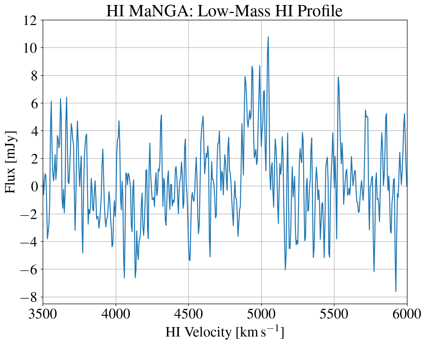
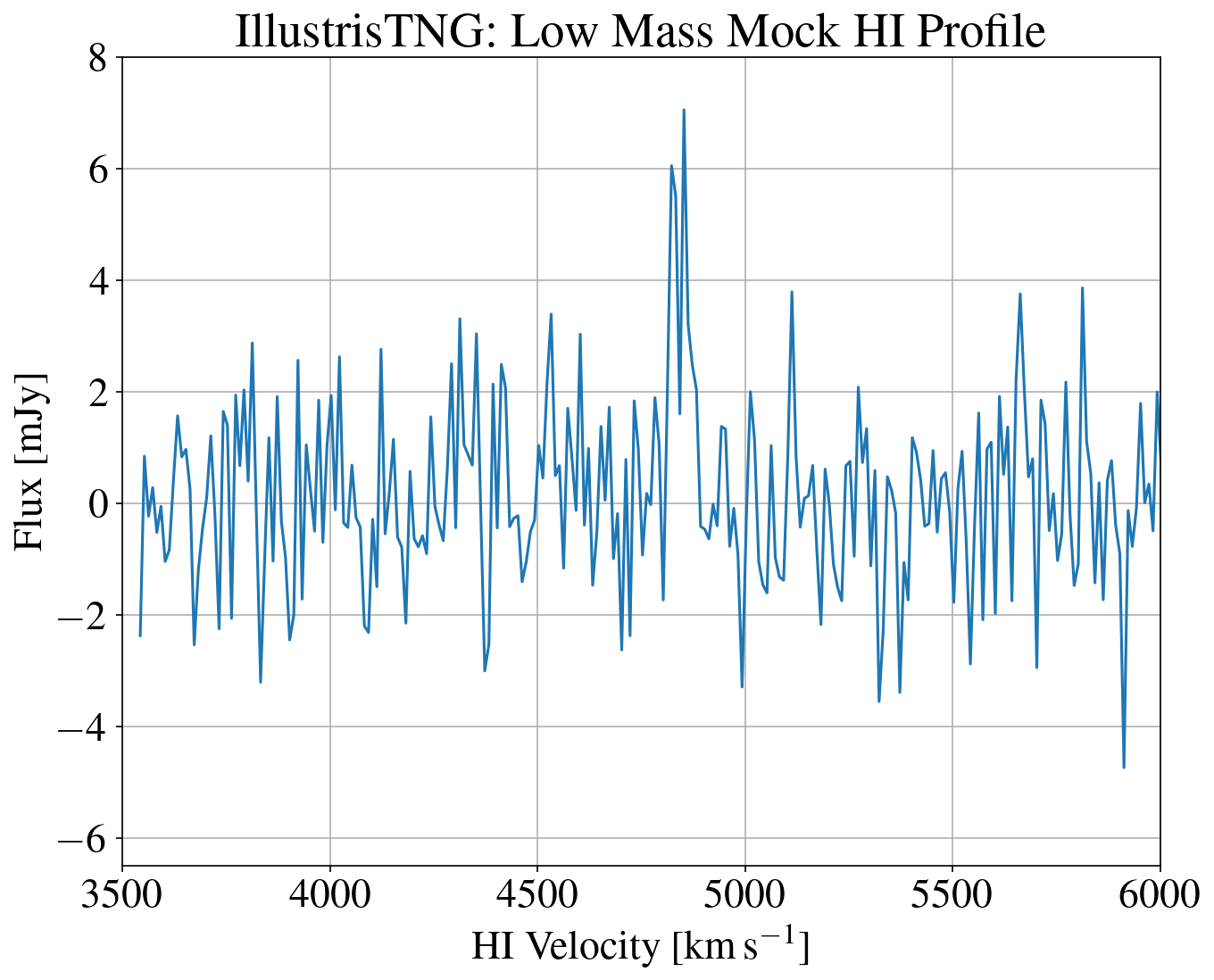
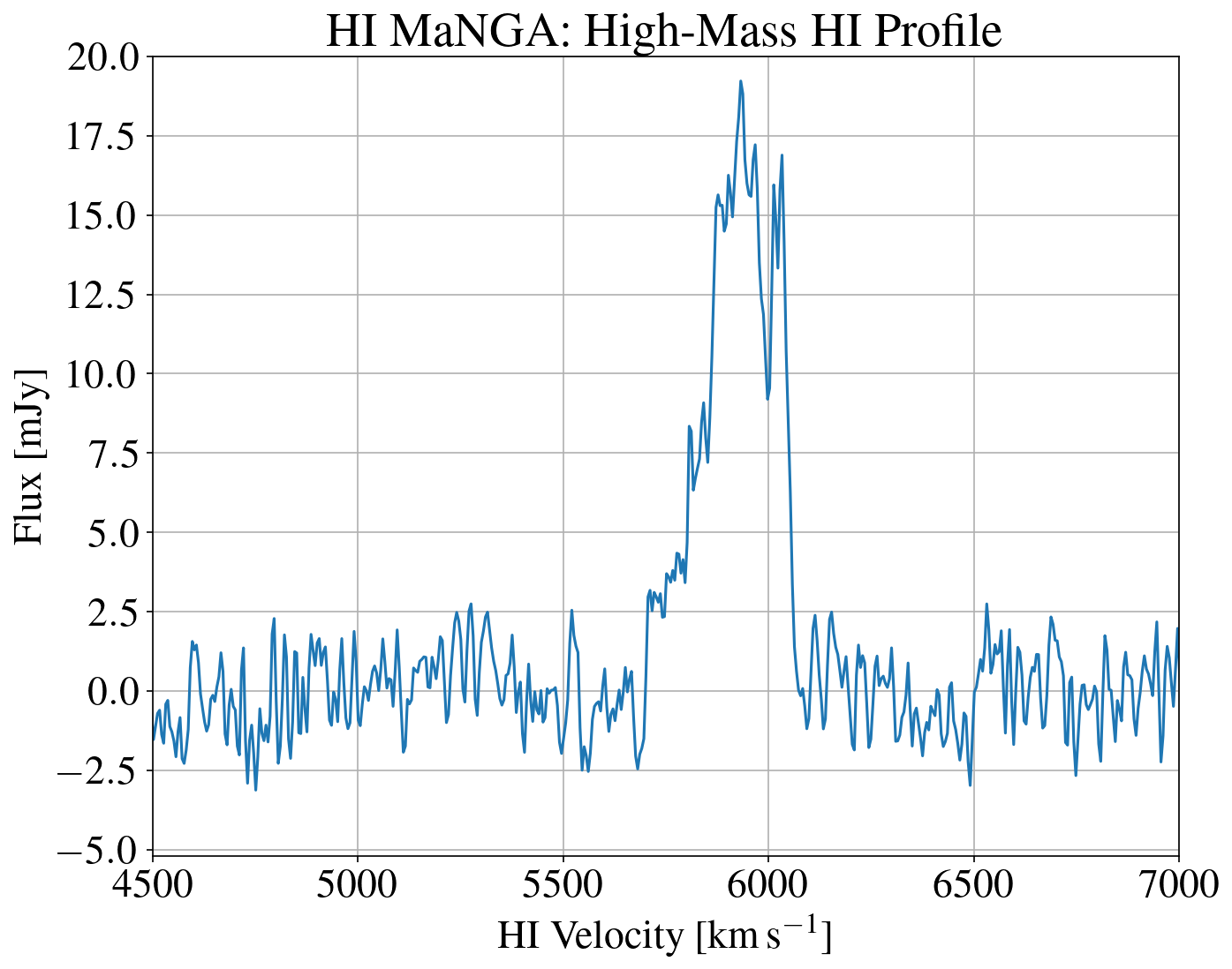
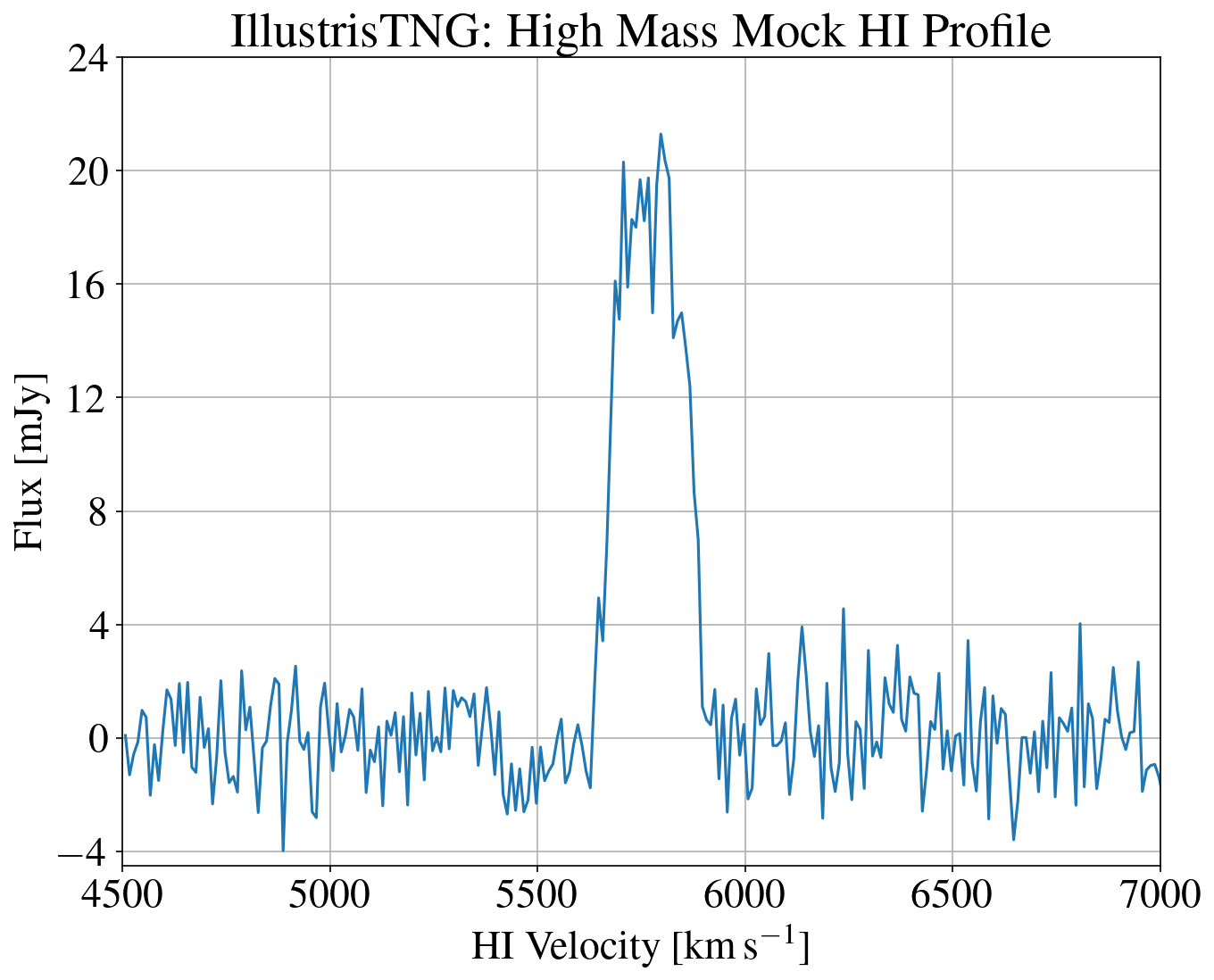
Figure 1: Sample matching HI profiles for low mass galaxies (MaNGA plateifu: 8937-6102 on top left and IllustrisTNG ID: 583726 on top right) and high mass galaxies (MaNGA plateifu: 8548-3702 on bottom left and IllustrisTNG ID: 586848 on bottom right)

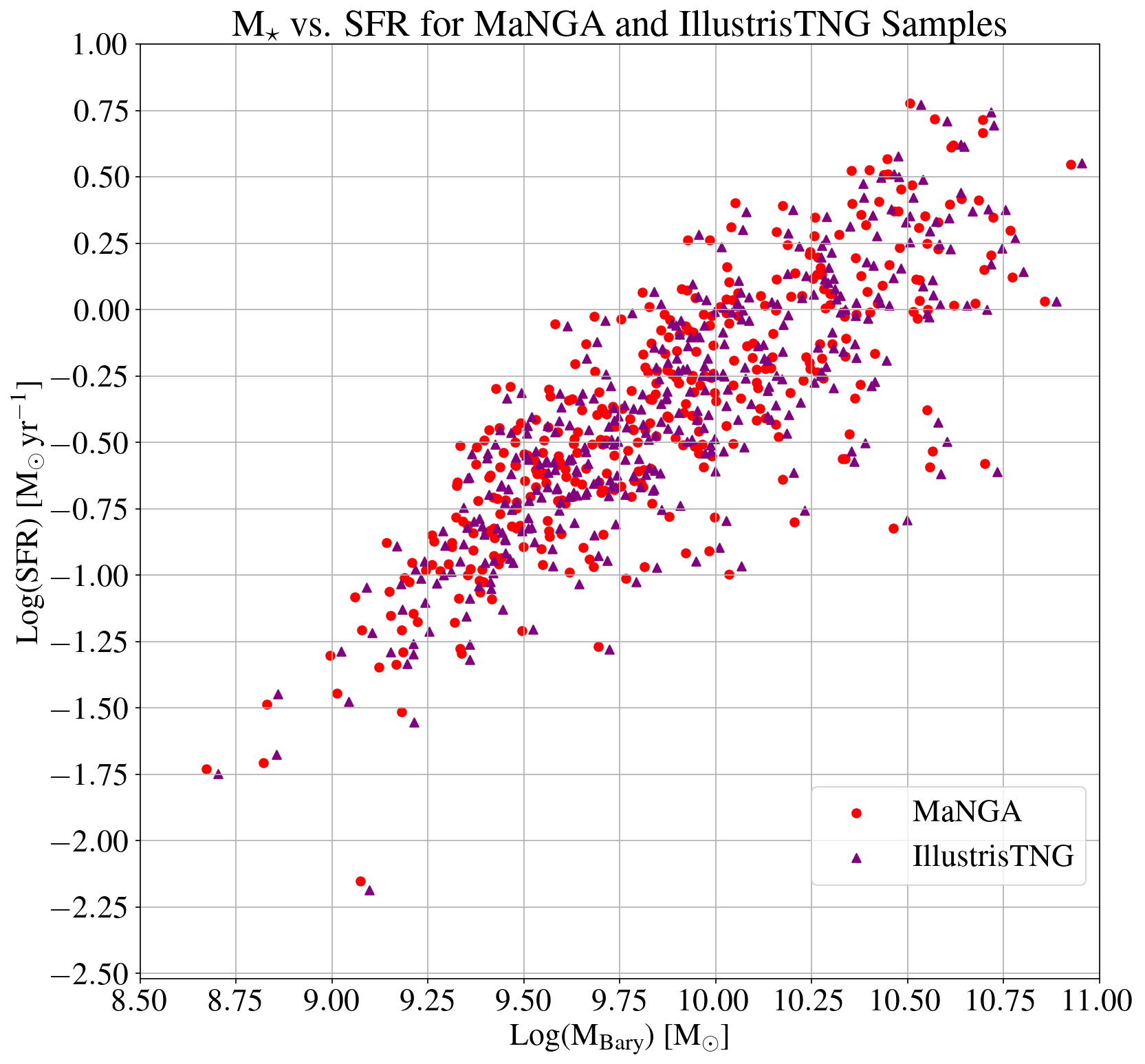
Figure 2: Stellar Mass vs. Star Formation Rate for the MaNGA and IllustrisTNG samples showing the similarity of the primary and control samples.

2.3 The Bayesian MCMC Linear Fitting Algorithm

A complication in calibrating the BTFR with the MaNGA data is fitting a line to data with significant observational scatter and/or strong outliers. This scatter is most likely a combination of intrinsic scatter and observational uncertainty. A $\Lambda$CDM cosmological framework predicts significant intrinsic scatter in the BTFR (Bradford et al., 2016), although the true level of intrinsic scatter is debated (McGaugh, 2012; Lelli et al., 2016b; Papastergis et al., 2016). The observational scatter could be caused by random measurement uncertainty as well as systematic effects, e.g., HI poorly tracing the rotation velocity due to it not filling the potential well of gas-poor galaxies (Lelli et al., 2016a) or other systematic variations in the relationship between HI linewidth and the “flat" part of the rotation curve (Verheijen, 2001).

To address potential complications when fitting a line to data with considerable scatter, we use a Bayesian Markov Chain Monte Carlo (MCMC) linear regression fitting algorithm based on the theano and PYMC3 modules in Python (The Theano Development Team et al., 2016; Salvatier et al., 2015). This algorithm identifies likely significant outliers and removes them from the data set prior to performing a linear fit to the remaining data. For for more details see Hogg et al. (2010); we use the implementation by Coleman Krawcyzk.

We add an additional variance prior and a corresponding standard deviation to account for the intrinsic scatter caused by intrinsic differences between individual galaxies. Accordingly, the model has five free parameters: slope, y-intercept, intrinsic scatter on outlier and inlier points, and measurement uncertainty. We use normal distributions as priors for the slope and y-intercept and inverse gamma functions for the intrinsic variance on the outlier and inlier points. We also change the target percentage that random walks will be added to the chain (called target_accept) from its default value of 0.8 to 0.999. This ensures that the algorithm only selects points along its random walk, which helps it converge.

The MCMC algorithm used in this work conducts fits which determine best fit linear parameters of $y$ vs. $x$ by minimizing the scatter in the $y$ direction. However, as there is no clear dependent variable in the BTFR, we prefer to treat the two variables symmetrically. Therefore, we use the MCMC algorithm to fit both rotation velocity vs. baryonic mass (forward fit) and baryonic mass vs. rotation velocity (inverse fit). We then combine these results into a final best-fit relation (bisector fit) using the bisector method described in Isobe et al. (1990).

3 Results

We now present the derived Baryonic Tully-Fisher relations for the observational MaNGA sample as well as the mock-observed (and simulated) IllustrisTNG samples. We show the forward, inverse, and bisector fits in all cases. Our analysis here always uses $V_{50}$ for the velocity variable. In Section 4.2, we will discuss how alternative velocity measurements can affect our results. To provide a comparison between relations derived from observational versus purely theoretical quantities, in Section  4.1 we also perform the same fitting routines on IllustrisTNG data but using $V_{\rm max}$, a rotation velocity measure derived directly from the simulations and not subject to measurement uncertainty. All derived best fit parameters and their associated uncertainties are provided in Table 1.

3.1 The MaNGA BTFR

We show the rotation velocity vs. baryonic mass (top left) baryonic mass vs. rotation velocity (top right) and the bisector fit (bottom) with rotation velocity on the horizontal axis and baryonic mass on the vertical axis for the MaNGA sample in Figure 3. The points that the Bayesian MCMC linear regression code determined have $>80\%$ probability of being outliers are plotted in red. We also show the 1-$\sigma$ best fit region, and the best fit lines in blue, and red respectively. The subplots show the residuals for each point using the same color criteria as for the main plot and a horizontal line at zero for reference.

The resulting bisector fit has a slope of 2.97 $\pm$ 0.18 with a y-intercept of $\log(M_{\rm bary}/M_{\odot})=4.04\pm$ 0.41.

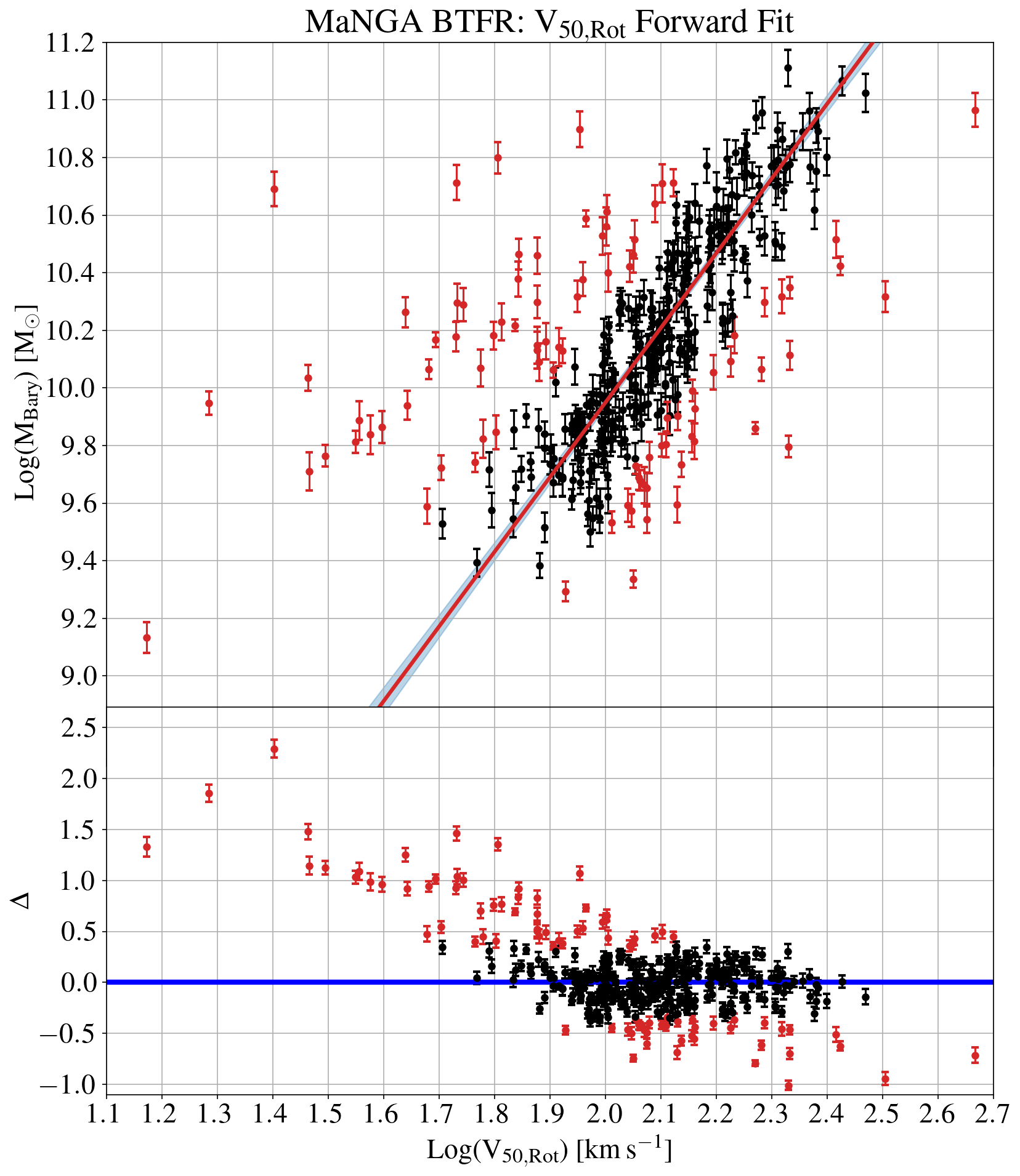
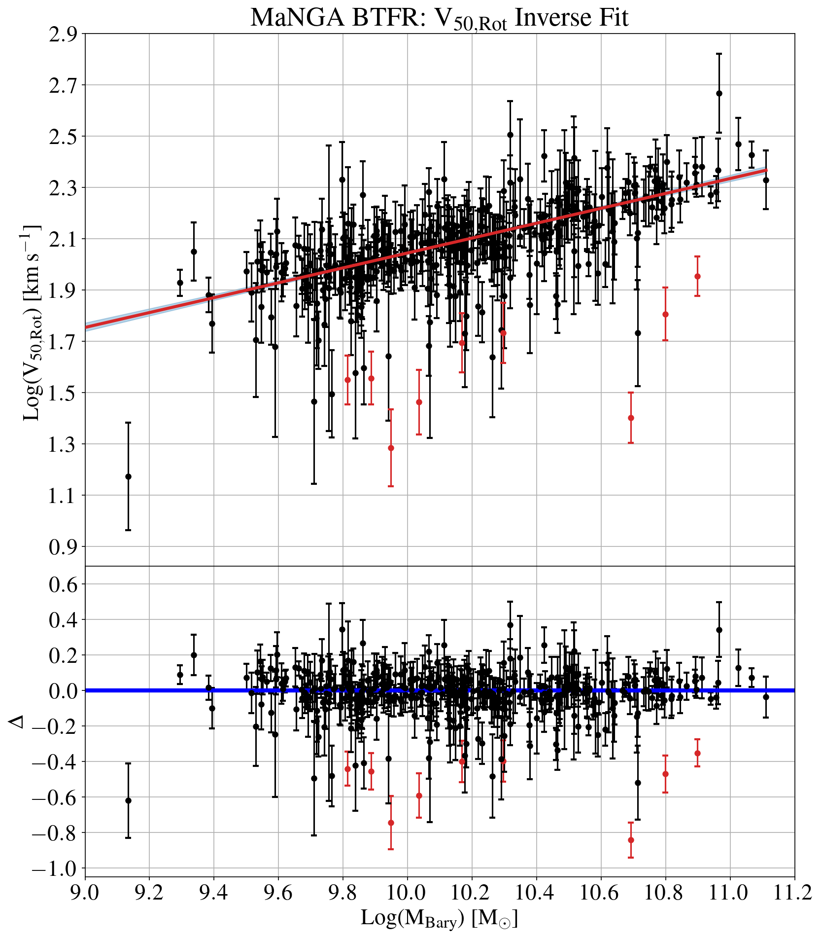
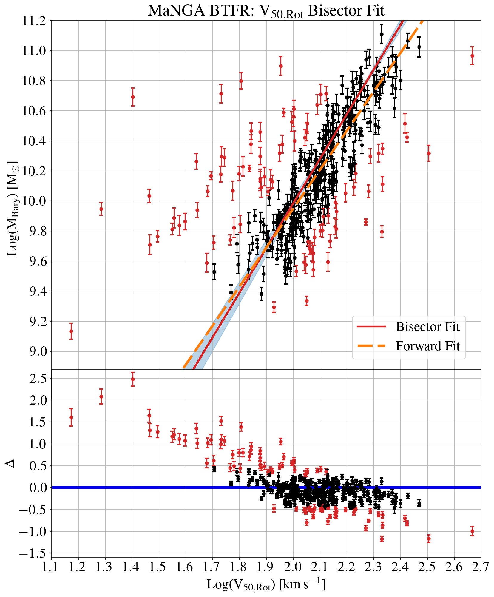
Figure 3: The MaNGA BTFR forward fit with rotation velocity on the horizontal axis and baryonic mass on the vertical axis (top left), the inverse fit with baryonic mass on the horizontal axis and rotation velocity on the vertical axis (top right), and the bisector fit with rotation velocity on the horizontal axis and baryonic mass on the vertical axis (bottom). The points that the Bayesian MCMC linear regression code determined have $>80\%$ probability of being an outlier are plotted in red. We also show the 1-$\sigma$ best fit region, and the best fit lines in blue, and red respectively. The subplots show the residuals for each point using the same color criteria as for the main plot and a horizontal line at zero for reference. The forward and bisector fits have 88 outliers and the inverse fit has 9 outliers. The best fit lines, clockwise from left, have slope 2.59 $\pm$ 0.09 with a y-intercept of 4.76 $\pm$ 0.19, slope of 3.44 $\pm$ 0.16 with a y-intercept of 2.95 $\pm$ 0.33, and 2.97 $\pm$ 0.18 with a y-intercept of 4.04 $\pm$ 0.41.

3.2 The IllustrisTNG BTFR

Figure 4 illustrates the mock observational data and resulting BTFR fit using IllustrisTNG. The plots show the same information as Figure 3, but for the IllustrisTNG mock-observed sample instead of the MaNGA sample. The resulting bisector fit has a slope of 2.94 $\pm$ 0.23 with a y-intercept of $\log(M_{\rm bary}/M_{\odot})=4.15\pm$ 0.44.

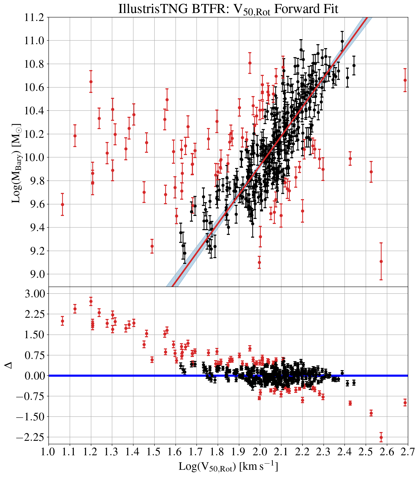
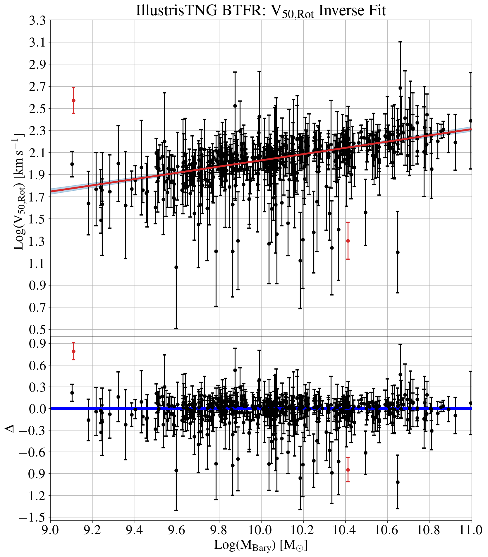
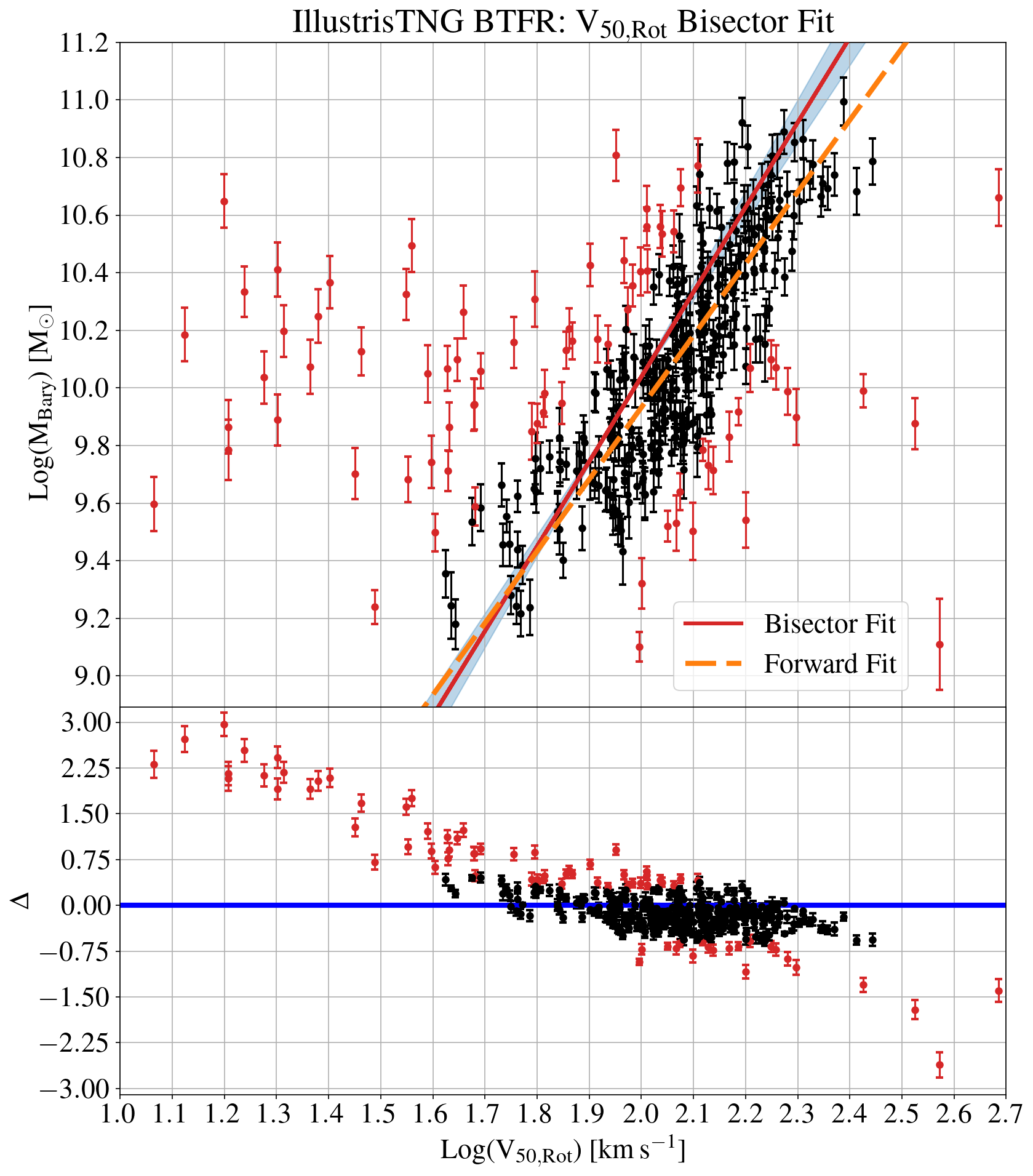
Figure 4: Same as Figure 3 but for the IllustrisTNG mock sample. The forward and bisector fits have 78 outliers and the inverse fit has 2 outliers. The best fit lines, clockwise from left, have slope 2.50 $\pm$ 0.13 with a y-intercept of 4.94 $\pm$ 0.28, slope of 3.56 $\pm$ 0.28 with a y-intercept of 2.78 $\pm$ 0.57, and 2.94 $\pm$ 0.23 with a y-intercept of 4.15 $\pm$ 0.44.

4 Discussion

MaNGA and IllustrisTNG produce BTFRs that agree within uncertainties, lending support to the idea that IllustrisTNG has created a galaxy population that obeys the observed relationship between mass and rotation velocity in the observed universe. We demonstrate this agreement by plotting both the MaNGA and IllustrisTNG BTFR bisector fits on the MaNGA data and the IllustrisTNG data, which are shown in Figure 5.

While we have made every effort to make a fair comparison between MaNGA and IllustrisTNG, some small differences remain which could lead to minor discrepancies between the resulting BTFRs. For example, the samples assume a slightly different cosmology and IMF. However, given that these factors impact mass estimates, but not 21cm linewidths, any offset should only be present in the BTFR zero points, not the slopes. Despite the expected differences, both slopes and intercepts agree within $1\sigma$. We expect this because systematic shifts due to assumed IMF and cosmology are smaller than typical errors on determinations of stellar mass.

In the following, we demonstrate the impact that using mock observations has on the calibration of the BTFR for simulated data. We also present a comparison of our results with other observational studies.

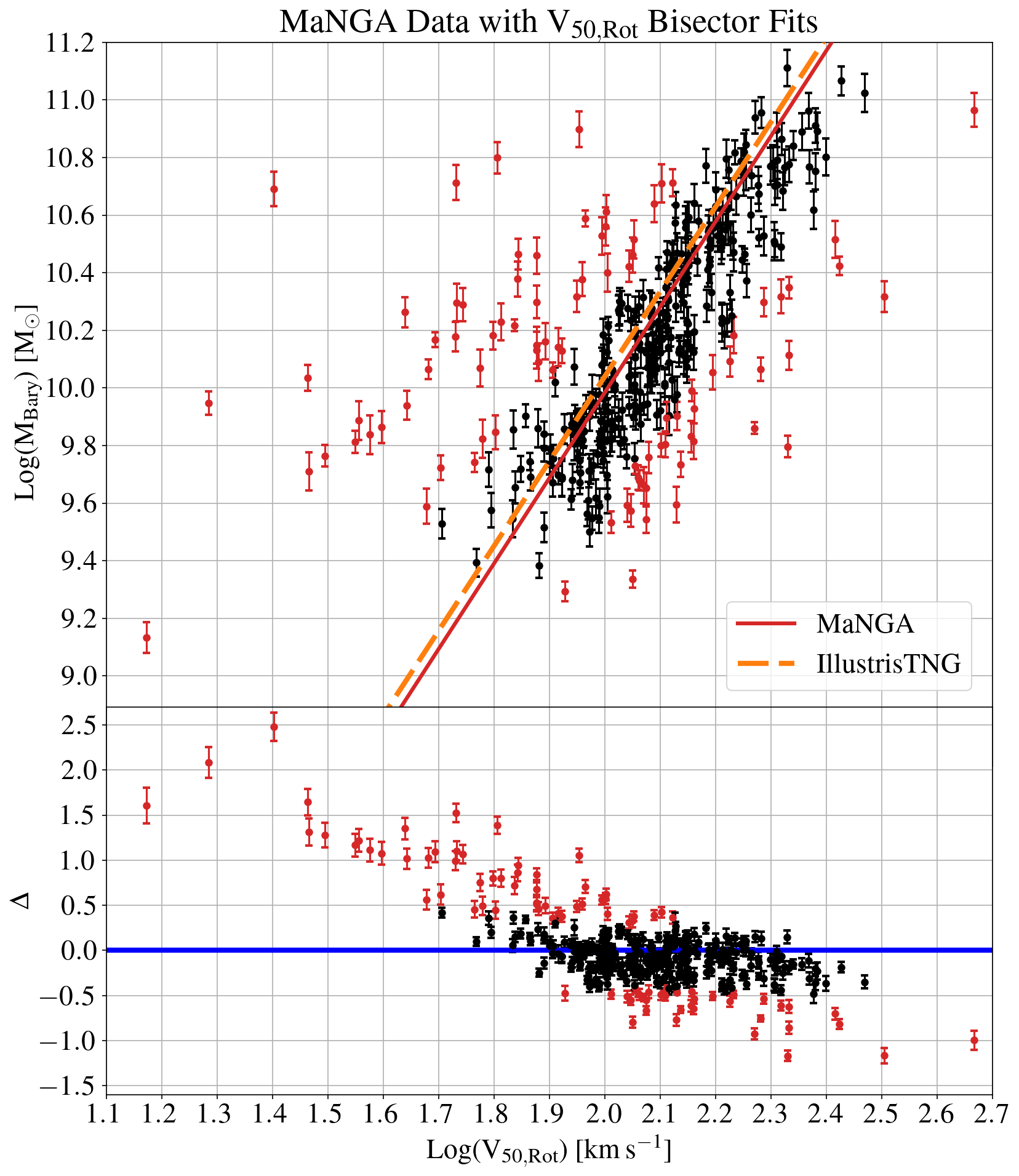
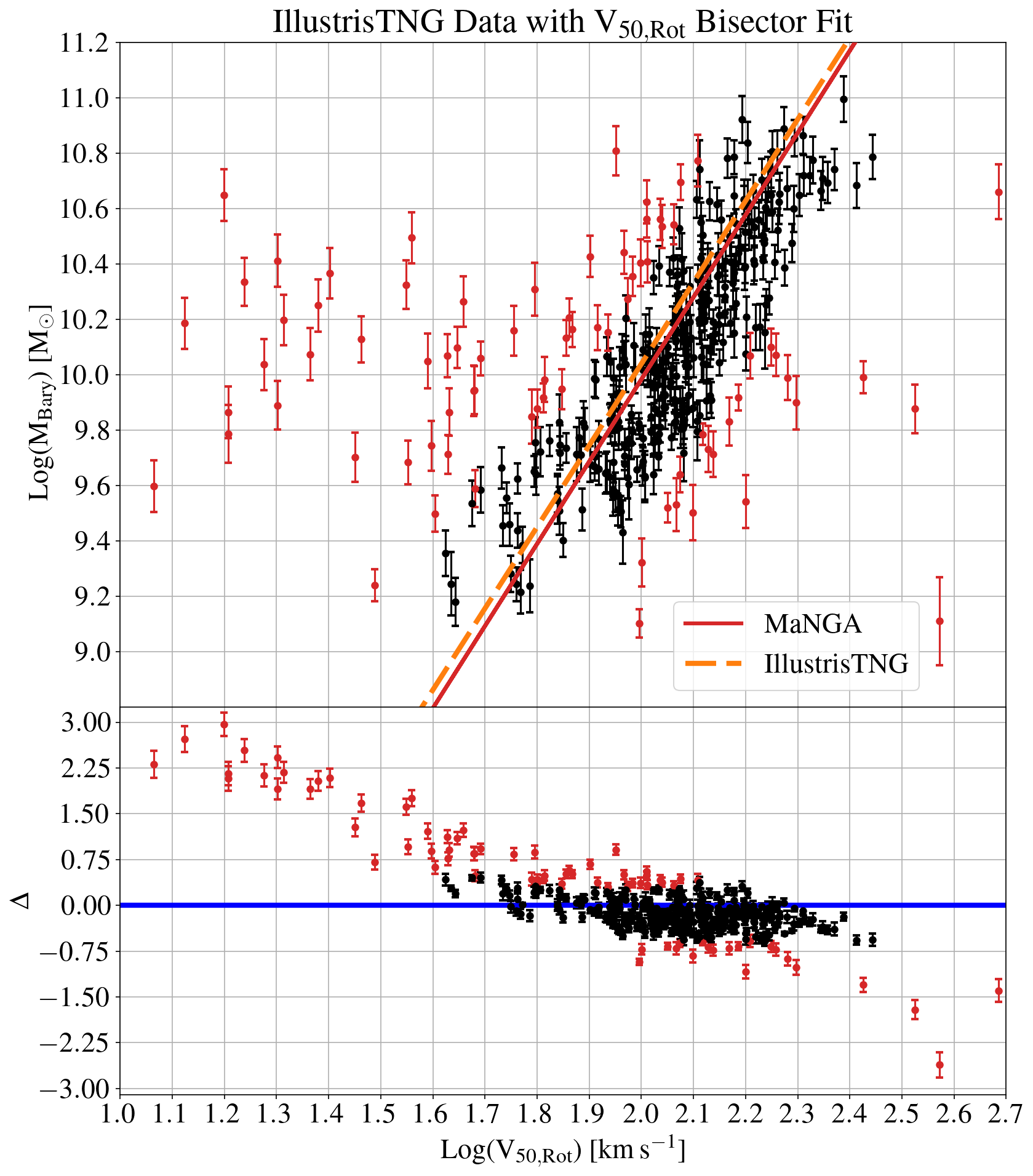
Figure 5: The MaNGA data (left) and IllustrisTNG (right) calculated using V_50,Rot with both the MaNGA (solid) and IllustrisTNG (dashed) V_50,Rot BTFR bisector fits overplotted. We use the same color criteria as for figures 3 and 4, except we do not show the respective 1-$\sigma$ regions in these plots for clarity. Rotation velocity is on the horizontal axis and baryonic mass is on the vertical axis. The MaNGA BTFR bisector fit has a slope of 2.97 $\pm$ 0.18 with a y-intercept of 4.04 $\pm$ 0.41 and the IllustrisTNG BTFR bisector fit has a slope of 2.94 $\pm$ 0.23 with a y-intercept of 4.15 $\pm$ 0.44.

4.1 The necessity of mock observations: the IllustrisTNG BTFR with rotation velocity directly from IllusrisTNG

A major emphasis of this work is the use of mock HI observations of IllustrisTNG galaxies to ensure a fair comparison with a real observational sample. We now demonstrate the impact and necessity for mock observations of simulated data when making comparisons with observational data. Specifically, we do not use the mock GBT observations (see Section 2.2.2). Instead, we create a BTFR using the rotational velocities extracted directly from IllustrisTNG and HI masses created through idealized observations that do not apply the GBT observational uncertainties. We employ the same bisector method used to derive the MaNGA and IllustisTNG BTFR’s with the mock observations. We show the rotation velocity vs. baryonic mass and baryonic mass vs. rotation velocity fits for the IllustrisTNG galaxies, as well as the corresponding bisector fit, in Figure 6 using the same color criteria as in Figures 3 and 4. The rotation velocity vs. baryonic mass fit has a slope of 3.47 $\pm$ 0.07 with a y-intercept of 2.61 $\pm$ 0.14 $\log_{10}M_{\odot}$. The baryonic mass vs. rotation velocity fit has a slope of 3.84 $\pm$ 0.08 with a y-intercept of 1.82 $\pm$ 0.17 $\log_{10}M_{\odot}$. The corresponding bisector fit has a slope of 3.65 $\pm$ 0.11 with a y-intercept of 2.25 $\pm$ 0.12 $\log_{10}M_{\odot}$ These results are also provided in Table 1. We note that the measurements from IllustrisTNG are known perfectly since they are simulated and consequently have zero uncertainty. Although this BTFR has less scatter and consequently smaller uncertainties, it notably does not agree with the MaNGA BTFR, showing a significantly steeper bisector slope. To emphasize this disagreement, we plot the MaNGA, IllustrisTNG mock-observed, and IllustrisTNG direct BTFR fits on the MaNGA data. This is shown in Figure 7 using the same color criteria as in Figures 3 and 4. There is no expectation that the BTFR based on theoretical maximum velocity should match that based on observed line width (e.g. see Lelli et al., 2019). We confirm here that they do not match, and therefore mock observations of simulations are important for matching with real observed relations.

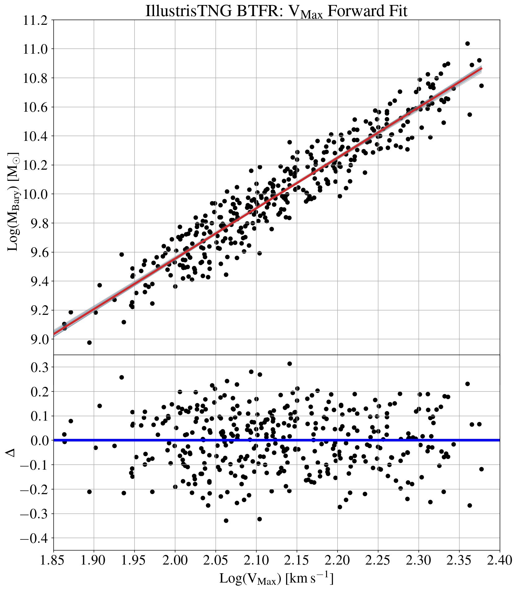
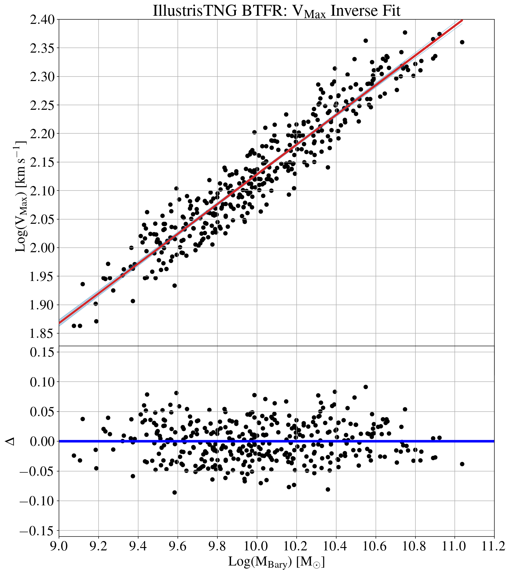
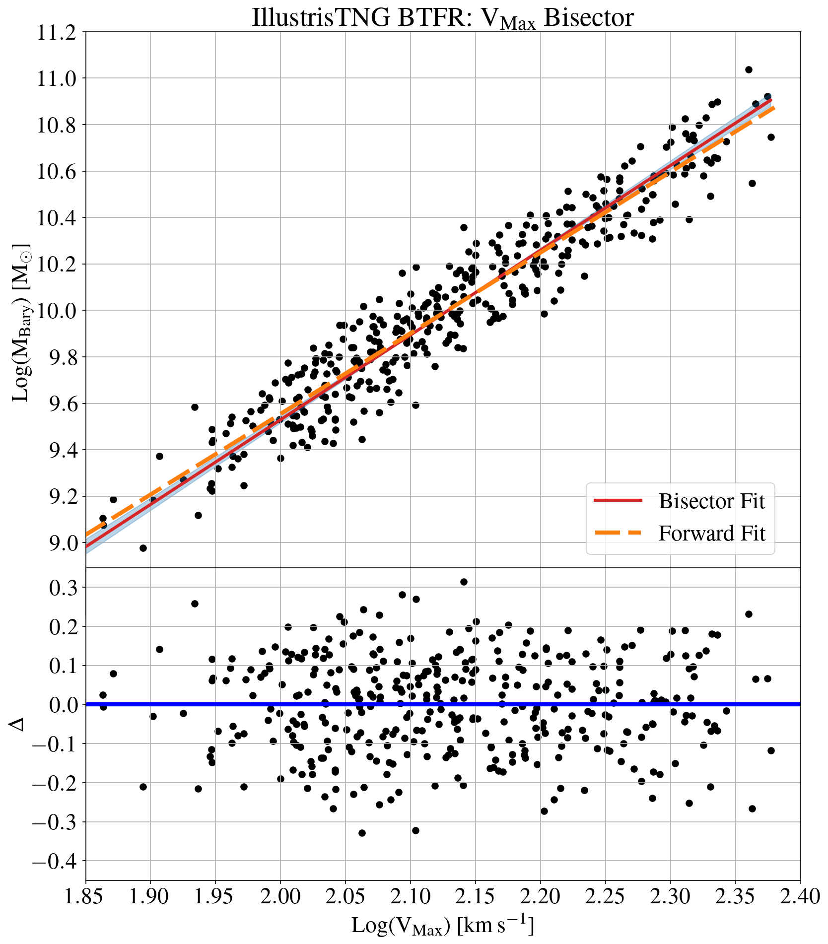
Figure 6: The IllustrisTNG BTFR with the IllustrisTNG rotation velocities directly rather than using mock observations. The top left shows rotation velocity on the horizontal axis and baryonic mass on the vertical axis. The top right shows baryonic mass on the horizontal axis and rotation velocity on the vertical axis. The bottom shows the bisector fit. We use the same color criteria as in Figures 3 and 4. The best fit lines, clockwise from left, have slope 3.47 $\pm$ 0.07 with a y-intercept of 2.61 $\pm$ 0.14, slope of 3.84 $\pm$ 0.08 with a y-intercept of 1.83 $\pm$ 0.17, and 3.65 $\pm$ 0.11 with a y-intercept of 2.25 $\pm$ 0.12. We note that the mass and rotation velocity measurements have zero uncertainty because they are taken directly from IllustrisTNG and are known perfectly since they are simulated. This BTFR does not agree with MaNGA, demonstrating the need for the mock observations to create a fair and consistent comparison between observation and theory.

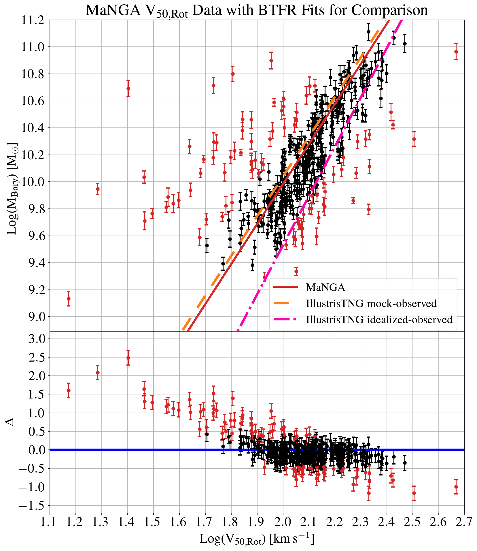
Figure 7: The MaNGA, IllustrisTNG mock-observed, and IllustrisTNG direct BTFR fits on the MaNGA data. The solid red line is the MaNGA BTFR fit. the dashed orange line is the IllustrisTNG mock-observed BTFR fit. The dash-dotted pink line is the BTFR directly from IllustrisTNG. This shows that the BTFR measured directly from IllustrisTNG does not agree the one from MaNGA but the mock observed IllustrisTNG BTFR does. This demonstrates the need for the mock observations to create a fair and consistent comparison between observation and theory.

4.2 A Comparison to the Literature

Due to the various definitions of rotation velocity, we can only accurately compare our results to other studies that also use linewidths (see Section 1 for details on these different definitions). The slope of the BTFR derived using linewidths in previous studies vary between 3 and 4 (Noordermeer & Verheijen, 2007; Avila-Reese et al., 2008; Gurovich et al., 2010; Zaritsky et al., 2014; Bradford et al., 2016; Brook et al., 2016; Papastergis et al., 2016; Lelli et al., 2019). The MaNGA and IllustrisTNG BTFR slopes are both low in comparison with the literature, but still consistent within uncertainties. The comparison with these authors is shown in Table 2.

There are additional differences between studies that could affect our comparisons, such as linewidth definition, turbulent velocity corrections, and sample definition. In this section, we test how these choices can affect our resulting BTFR. Our alternative BTFR fits are given in Table 1.

Many studies represent velocity using $W_{20}$, rather than $W_{50}$. To test the impact of this choice, we calculate the best-fit BTFR using $V_{20}$ instead of $V_{50}$. We find using $V_{20}$ has negligible impact on the the MaNGA BTFR. The IllustrisTNG BTFR slope increases mildly by 0.15, which is within the uncertainties of the original fit.

While it is common for measured 21cm linewidths to be corrected for instrumental broadening (Springob et al., 2005), many previous studies do not always apply a correction for turbulent motions. We explore whether our shallow slope compared with the literature can be attributed to the unequal influence of turbulence across all parameter space. Our corrected linewidths (see Eq. 6) include a constant factor, $\Delta t$, which is the turbulent velocity correction. As this factor is constant, it has a larger effect on less massive galaxies which host smaller linewidths, preferentially decreasing the rotation velocity of smaller galaxies and possibly biasing the best fit to shallower slopes. To test its impact, we reran our fits without the turbulence correction, but found it has only a marginal effect on the derived BTFR and consequently does not account for our shallow slope, as shown in Table 1.

Similarly, while previous studies are often explicitly limited to disk galaxies, we have made no morphology cut, although our sample will be biased towards disk galaxies by design of requiring HI detections. Nonetheless, there is a possibility that including early-type galaxies, which have less rotational support, could be responsible for our shallower BTFR slope. To test this possibility, we employ the $\mu_{\Delta}$ parameter of  Kannappan2013 to identify and reject spheroid dominated galaxies from our fits. The $\mu_{\Delta}$ quantity is a stellar mass surface density contrast between the regions within and external to $r_{50}$, similar to a concentration index, but providing a cleaner separation between early- and late-type galaxies (Moffett et al., 2015). We exclude early-type galaxies by rejecting all galaxies with $\mu_{\Delta}>9.5$. We note that this cut is based on the sample in Kannappan et al. (2013), and we assume it is valid for our sample as well. Limiting our sample in this way has negligible impact on the resulting slopes for our MaNGA sample. The slopes derived from the IllustrisTNG sample are somewhat higher by $\sim 0.2$. However, the MaNGA and IllustrisTNG samples still provide results that agree with each other within the uncertainties.

Type of BTFR Fit	$\Delta t$ Correction?	Sample Size	Number of Outliers	Slope†	Zero Point†
					$\log{M_{\rm Bary}/M_{\odot}}$
Main Comparison ($V_{\rm 50,Rot}$ and $M_{\rm Bary}$)
MaNGA: Forward	Yes	377	88	2.59 $\pm$ 0.09	4.76 $\pm$ 0.19
MaNGA: Inverse	Yes	377	9	3.44 $\pm$ 0.16	2.95 $\pm$ 0.33
MaNGA: Bisector	Yes	377	88	2.97 $\pm$ 0.18	4.04 $\pm$ 0.41
IllustrisTNG: Forward	Yes	377	78	2.50 $\pm$ 0.13	4.94 $\pm$ 0.28
IllustrisTNG: Inverse	Yes	377	2	3.56 $\pm$ 0.28	2.78 $\pm$ 0.57
IllustrisTNG: Bisector	Yes	377	78	2.94 $\pm$ 0.23	4.15 $\pm$ 0.44
Without mock observations ($V_{\rm max}$ and $M_{\rm Bary}$)
IllustrisTNG: Forward	N/A	377	0	3.47 $\pm$ 0.07	2.61 $\pm$ 0.14
IllustrisTNG: Inverse	N/A	377	0	3.84 $\pm$ 0.08	1.82 $\pm$ 0.17
IllustrisTNG: Bisector	N/A	377	0	3.65 $\pm$ 0.11	2.25 $\pm$ 0.12
Testing HI width choice ($V_{\rm 20,Rot}$ and $M_{\rm Bary}$)
MaNGA: Forward	Yes	377	40	2.51 $\pm$ 0.17	4.78 $\pm$ 0.37
MaNGA: Inverse	Yes	377	5	3.73 $\pm$ 0.18	2.17 $\pm$ 0.40
MaNGA: Bisector	Yes	377	40	3.01 $\pm$ 0.17	3.73 $\pm$ 0.36
IllustrisTNG: Forward	Yes	377	39	2.58 $\pm$ 0.10	4.85 $\pm$ 0.22
IllustrisTNG: Inverse	Yes	377	11	3.82 $\pm$ 0.26	2.22 $\pm$ 0.55
IllustrisTNG: Bisector	Yes	377	39	3.09 $\pm$ 0.26	3.68 $\pm$ 0.51
Testing turbulence corrections ($V_{\rm 50,Rot}$ and $M_{\rm Bary}$)
MaNGA: Forward	No	377	87	2.75 $\pm$ 0.10	4.39 $\pm$ 0.21
MaNGA: Inverse	No	377	7	3.57 $\pm$ 0.17	2.64 $\pm$ 0.36
MaNGA: Bisector	No	377	87	3.11 $\pm$ 0.23	3.70 $\pm$ 0.40
IllustrisTNG: Forward	No	377	70	2.48 $\pm$ 0.20	4.96 $\pm$ 0.42
IllustrisTNG: Inverse	No	377	2	3.74 $\pm$ 0.31	2.36 $\pm$ 0.63
IllustrisTNG: Bisector	No	377	70	2.97 $\pm$ 0.22	4.12 $\pm$ 0.60
Morphology cut, $\mu_{\Delta}<9.5$ to select disks ($V_{\rm 50,Rot}$ and $M_{\rm Bary}$)
MaNGA: Forward	Yes	368	86	2.59 $\pm$ 0.09	4.77 $\pm$ 0.19
MaNGA: Inverse	Yes	368	9	3.47 $\pm$ 0.16	2.91 $\pm$ 0.34
MaNGA: Bisector	Yes	368	86	2.97 $\pm$ 0.19	4.05 $\pm$ 0.41
IllustrisTNG: Forward	Yes	330	72	2.71 $\pm$ 0.12	4.47 $\pm$ 0.25
IllustrisTNG: Inverse	Yes	330	0	3.68 $\pm$ 0.30	2.51 $\pm$ 0.63
IllustrisTNG: Bisector	Yes	330	72	3.13 $\pm$ 0.22	3.73 $\pm$ 0.44

Table 1: Our various BTFR fits, for V₅₀ and V₂₀, testing the impact of HI width choice, use of mock observations, a morphological $\mu_{\Delta}$ cut and turbulence corrections.^†The inverse fits are initially calculated as $V_{\rm Rot}=m^{\prime}M_{\rm bary}+b^{\prime}$, but we present the slope and zero points after converting the results in the “forward fit" form of $M_{\rm bary}=mV_{\rm rot}+b$, where $m=1/m^{\prime}$ and $b=-b^{\prime}/m^{\prime}$. For all of the permutations, the MaNGA and IllustrisTNG fits agree within uncertainties.

Line	$\Delta t$	Slope	Reference
width	correction?
$W_{\rm F50}$	Yes	2.97 $\pm$ 0.18	This work (MaNGA data/bisector)
$W_{\rm F50}$	Yes	2.97 $\pm$ 0.22	This work (Illustris TNG/bisector)
$W_{\rm F20}$	Yes	3.01 $\pm$ 0.17	This work (MaNGA data/bisector)
$W_{\rm F20}$	Yes	3.09 $\pm$ 0.26	This work (Illustris TNG/bisector)
$W_{\rm 20}$	Yes	$3.27\pm 0.13$	Avila-Reese et al. (2008)
$W_{\rm 50}$	Yes	3.5 $\pm$ 0.2	Zaritsky et al. (2014)
$W_{\rm M50}/2$	Yes	3.62 $\pm$ 0.09	Lelli et al. (2019)
$W_{\rm 50}/2$	No	2.70	Brook et al. (2016)
$W_{\rm 50}$	No?	2.80 $\pm$ 0.14	Ponomareva et al. (2018)
$W_{\rm F50}$	No	2.97 $\pm$ 0.29	This work (IllustrisTNG/bisector)
$W_{\rm 20}$	No	$3.04\pm 0.08$	Noordermeer & Verheijen (2007)
$W_{\rm F50}$	No	3.11 $\pm$ 0.19	This work (MaNGA data/bisector)
$W_{\rm 20}/2$	No	3.13	Brook et al. (2016)
$W_{\rm 20}$	No	$3.20\pm 0.10$	Gurovich et al. (2010)
$W_{\rm 20}$	No	3.24 $\pm$ 0.05	Bradford et al. (2016)
$W_{\rm 50}/2$	No	3.75 $\pm$ 0.11	Papastergis et al. (2016)
$W_{\rm P20}/2$	No	3.85 $\pm$ 0.09	Lelli et al. (2019)

Table 2: Our various BTFR fits showing that our slopes are shallow compared with some from the literature also using linewidths. $W_{20}$ is the linewidth at 20% of its peak and $W_{50}$ is the linewidth at 50% of its peak.

5 Conclusions and Future Directions

We compare the observed BTFR using SDSS-IV MaNGA and HI-MaNGA observations to a simulated one from IllustrisTNG. We perform mock 21 cm observations on galaxies from IllustrisTNG, ensuring a fair comparison between the observed galaxies with observational limitations, biases, and uncertainties and the simulation without those constraints, as well as to minimize disagreements caused by different measurement methods. We report a MaNGA BTFR slope of 2.97 $\pm$ 0.18 with a y-intercept of 4.04 $\pm$ 0.41 and an IllustrisTNG BTFR slope of 2.94 $\pm$ 0.23 with a y-intercept of 4.15 $\pm$ 0.44. Thus, MaNGA and IllustrisTNG produce BTFRs that agree within uncertainties, suggesting IllustrisTNG has created a galaxy population that accurately represents that of the real universe when judged by BTFR.

To demonstrate the importance of mock observations on simulated data, we also create a BTFR using rotation velocity directly from IllustrisTNG and demonstrate that it is necessary to create the BTFR in a fair and consistent way between observation and theory when comparing the two. This is noteworthy because simulations have historically struggled to reproduce observed galaxy scaling relations such as the BTFR (Somerville & Davé, 2015).

IllustrisTNG is used to simulate a wide range of cosmological and extra-galactic phenomena, including thermodynamic structure in galaxy clusters (Barnes et al., 2018), the large-scale distribution of highly ionized metals (Artale et al., 2021), dark matter halo formation (Hearin et al., 2021), the effect of galaxy mergers on galaxy evolution (Hani et al., 2020), the dark matter and the star formation in galaxies (Lovell et al., 2018; Tacchella et al., 2019), the properties and distribution of bars in spiral galaxies (Zhao et al., 2020), supermassive black hole formation and feedback (Weinberger et al., 2018), and even fast radio bursts (Zhang et al., 2021) and binary neutron star mergers (Rose et al., 2021). This demonstration that IllustrisTNG accurately recreates the observed BTFR gives us more confidence that those phenomena simulated with IllustrisTNG actually reflect reality.

There are a number of avenues for expanding upon our analysis. This work primarily focused on the treatment of single dish 21cm spectra, and future work may benefit from incorporating and comparing results from alternative linewidth estimation algorithms, as has been done other studies (Trachternach et al., 2009; McGaugh, 2012; Desmond & Wechsler, 2015; Bradford et al., 2016; Brook et al., 2016; Lelli et al., 2019; Glowacki et al., 2020). Estimating linewidths using measured rotation curves from MaNGA IFU spectroscopy, and mock rotation curves from IllustrisTNG galaxies is a natural next step. Lastly, future analysis may benefit from a careful homogenization in the methods used to calculate stellar masses in MaNGA and IllustrisTNG, in which mock spectrophotometry of IllustrisTNG galaxies are generated and passed through the same programs used to estimate the stellar masses in the observational data. Such analyses should be possible thanks to routines that can postprocess simulated data into observed spectra (Torrey et al., 2015). More HI-MaNGA data is coming soon, which will give us a larger data set to perform these analyses.

Data Availability

The HI-MaNGA catalog used in this study can be found at https://greenbankobservatory.org/science/gbt-surveys/hi-manga/. The MaNGA MPL-10 data products can be generated by the public using the raw data (available at https://www.sdss.org/dr16/manga/manga-data/data-access/) with DRP v3.0.1 and Pipe3D v3.0.1. IllustrisTNG files are available from https://www.tng-project.org/data/ and mock HI data cubes can be recreated using the Martini package (https://github.com/kyleaoman/martini).

References

- Andersen & Bershady (2003) Andersen D. R., Bershady M. A., 2003, ApJ, 599, L79
- Artale et al. (2021) Artale M. C., et al., 2021, arXiv e-prints, p. arXiv:2102.01092
- Astropy Collaboration et al. (2013) Astropy Collaboration et al., 2013, A&A, 558, A33
- Astropy Collaboration et al. (2018) Astropy Collaboration et al., 2018, AJ, 156, 123
- Avila-Reese et al. (2008) Avila-Reese V., Zavala J., Firmani C., Hernández-Toledo H. M., 2008, AJ, 136, 1340
- Barnes et al. (2018) Barnes D. J., et al., 2018, MNRAS, 481, 1809
- Blanton et al. (2017) Blanton M. R., et al., 2017, AJ, 154, 28
- Blitz & Rosolowsky (2006) Blitz L., Rosolowsky E., 2006, ApJ, 650, 933
- Bolatto et al. (2013) Bolatto A. D., Wolfire M., Leroy A. K., 2013, ARA&A, 51, 207
- Bradford et al. (2016) Bradford J. D., Geha M. C., van den Bosch F. C., 2016, ApJ, 832, 11
- Brook et al. (2016) Brook C. B., Santos-Santos I., Stinson G., 2016, MNRAS, 459, 638
- Bundy et al. (2015) Bundy K., et al., 2015, ApJ, 798, 7
- Catinella et al. (2005) Catinella B., Haynes M. P., Giovanelli R., 2005, AJ, 130, 1037
- Catinella et al. (2018) Catinella B., et al., 2018, MNRAS, 476, 875
- Courteau et al. (2003) Courteau S., Andersen D. R., Bershady M. A., MacArthur L. A., Rix H.-W., 2003, ApJ, 594, 208
- Desmond & Wechsler (2015) Desmond H., Wechsler R. H., 2015, MNRAS, 454, 322
- Diamond-Stanic et al. (2016) Diamond-Stanic A. M., Coil A. L., Moustakas J., Tremonti C. A., Sell P. H., Mendez A. J., Hickox R. C., Rudnick G. H., 2016, ApJ, 824, 24
- Drory et al. (2015) Drory N., et al., 2015, AJ, 149, 77
- Ferrero et al. (2017) Ferrero I., et al., 2017, MNRAS, 464, 4736
- Glowacki et al. (2020) Glowacki M., Elson E., Davé R., 2020, MNRAS, 498, 3687
- Glowacki et al. (2021) Glowacki M., Elson E., Davé R., 2021, MNRAS, 507, 3267
- Gunn et al. (2006) Gunn J. E., et al., 2006, AJ, 131, 2332
- Gurovich et al. (2010) Gurovich S., Freeman K., Jerjen H., Staveley-Smith L., Puerari I., 2010, AJ, 140, 663
- Hani et al. (2020) Hani M. H., Gosain H., Ellison S. L., Patton D. R., Torrey P., 2020, MNRAS, 493, 3716
- Harris et al. (2020) Harris C. R., et al., 2020, Nature, 585, 357
- Haynes et al. (2018) Haynes M. P., et al., 2018, ApJ, 861, 49
- Hearin et al. (2021) Hearin A. P., Chaves-Montero J., Becker M. R., Alarcon A., 2021, arXiv e-prints, p. arXiv:2105.05859
- Hogg et al. (2010) Hogg D. W., Bovy J., Lang D., 2010, arXiv e-prints, p. arXiv:1008.4686
- Hunter (2007) Hunter J. D., 2007, Computing in Science and Engineering, 9, 90
- Isobe et al. (1990) Isobe T., Feigelson E. D., Akritas M. G., Babu G. J., 1990, ApJ, 364, 104
- Kannappan & Gawiser (2007) Kannappan S. J., Gawiser E., 2007, ApJ, 657, L5
- Kannappan et al. (2013) Kannappan S. J., et al., 2013, ApJ, 777, 42
- Law et al. (2015) Law D. R., et al., 2015, AJ, 150, 19
- Law et al. (2016) Law D. R., et al., 2016, AJ, 152, 83
- Law et al. (2021) Law D. R., et al., 2021, AJ, 161, 52
- Lelli et al. (2015) Lelli F., et al., 2015, A&A, 584, A113
- Lelli et al. (2016a) Lelli F., McGaugh S. S., Schombert J. M., 2016a, ApJ, 816, L14
- Lelli et al. (2016b) Lelli F., McGaugh S. S., Schombert J. M., Pawlowski M. S., 2016b, ApJ, 827, L19
- Lelli et al. (2019) Lelli F., McGaugh S. S., Schombert J. M., Desmond H., Katz H., 2019, MNRAS, 484, 3267
- Leroy et al. (2013) Leroy A. K., et al., 2013, AJ, 146, 19
- Lovell et al. (2018) Lovell M. R., et al., 2018, MNRAS, 481, 1950
- Marinacci et al. (2018) Marinacci F., et al., 2018, MNRAS, 480, 5113
- Masters et al. (2006) Masters K. L., Springob C. M., Haynes M. P., Giovanelli R., 2006, ApJ, 653, 861
- Masters et al. (2014) Masters K. L., Crook A., Hong T., Jarrett T. H., Koribalski B. S., Macri L., Springob C. M., Staveley-Smith L., 2014, MNRAS, 443, 1044
- Masters et al. (2019) Masters K. L., et al., 2019, MNRAS, 488, 3396
- McGaugh (2012) McGaugh S. S., 2012, AJ, 143, 40
- McGaugh & Schombert (2015) McGaugh S. S., Schombert J. M., 2015, ApJ, 802, 18
- McGaugh et al. (2000) McGaugh S. S., Schombert J. M., Bothun G. D., de Blok W. J. G., 2000, ApJ, 533, L99
- McGaugh et al. (2020) McGaugh S. S., Lelli F., Schombert J. M., 2020, Research Notes of the American Astronomical Society, 4, 45
- Meyer et al. (2008) Meyer M. J., Zwaan M. A., Webster R. L., Schneider S., Staveley-Smith L., 2008, MNRAS, 391, 1712
- Milgrom (1983) Milgrom M., 1983, ApJ, 270, 365
- Moffett et al. (2015) Moffett A. J., Kannappan S. J., Berlind A. A., Eckert K. D., Stark D. V., Hendel D., Norris M. A., Grogin N. A., 2015, ApJ, 812, 89
- Naiman et al. (2018) Naiman J. P., et al., 2018, MNRAS, 477, 1206
- Nelson et al. (2018) Nelson D., et al., 2018, MNRAS, 475, 624
- Noordermeer & Verheijen (2007) Noordermeer E., Verheijen M. A. W., 2007, MNRAS, 381, 1463
- Ogle et al. (2019) Ogle P. M., Jarrett T., Lanz L., Cluver M., Alatalo K., Appleton P. N., Mazzarella J. M., 2019, ApJ, 884, L11
- Oman et al. (2019) Oman K. A., Marasco A., Navarro J. F., Frenk C. S., Schaye J., Benítez-Llambay A., 2019, MNRAS, 482, 821
- Papastergis et al. (2016) Papastergis E., Adams E. A. K., van der Hulst J. M., 2016, A&A, 593, A39
- Pillepich et al. (2018a) Pillepich A., et al., 2018a, MNRAS, 473, 4077
- Pillepich et al. (2018b) Pillepich A., et al., 2018b, MNRAS, 475, 648
- Ponomareva et al. (2018) Ponomareva A. A., Verheijen M. A. W., Papastergis E., Bosma A., Peletier R. F., 2018, MNRAS, 474, 4366
- Rahmati et al. (2013) Rahmati A., Pawlik A. H., Raičević M., Schaye J., 2013, MNRAS, 430, 2427
- Rose et al. (2021) Rose J. C., Torrey P., Lee K. H., Bartos I., 2021, ApJ, 909, 207
- Sales et al. (2017) Sales L. V., et al., 2017, MNRAS, 464, 2419
- Salpeter (1955) Salpeter E. E., 1955, ApJ, 121, 161
- Salvatier et al. (2015) Salvatier J., Wiecki T., Fonnesbeck C., 2015, arXiv e-prints, p. arXiv:1507.08050
- Sánchez et al. (2016a) Sánchez S. F., et al., 2016a, Rev. Mex. Astron. Astrofis., 52, 21
- Sánchez et al. (2016b) Sánchez S. F., et al., 2016b, Rev. Mex. Astron. Astrofis., 52, 171
- Sánchez et al. (2018) Sánchez S. F., et al., 2018, Rev. Mex. Astron. Astrofis., 54, 217
- Schaye et al. (2015) Schaye J., et al., 2015, MNRAS, 446, 521
- Smee et al. (2013) Smee S. A., et al., 2013, AJ, 146, 32
- Somerville & Davé (2015) Somerville R. S., Davé R., 2015, ARA&A, 53, 51
- Sorce et al. (2016) Sorce J. G., Creasey P., Libeskind N. I., 2016, MNRAS, 455, 2644
- Springel (2010) Springel V., 2010, MNRAS, 401, 791
- Springel et al. (2018) Springel V., et al., 2018, MNRAS, 475, 676
- Springob et al. (2005) Springob C. M., Haynes M. P., Giovanelli R., Kent B. R., 2005, ApJS, 160, 149
- Stark et al. (2009) Stark D. V., McGaugh S. S., Swaters R. A., 2009, AJ, 138, 392
- Stark et al. (2021) Stark D. V., et al., 2021, MNRAS, 503, 1345
- Tacchella et al. (2019) Tacchella S., et al., 2019, MNRAS, 487, 5416
- The Theano Development Team et al. (2016) The Theano Development Team et al., 2016, arXiv e-prints, p. arXiv:1605.02688
- Torrey et al. (2015) Torrey P., et al., 2015, MNRAS, 447, 2753
- Trachternach et al. (2009) Trachternach C., de Blok W. J. G., McGaugh S. S., van der Hulst J. M., Dettmar R. J., 2009, A&A, 505, 577
- Tully & Courtois (2012) Tully R. B., Courtois H. M., 2012, ApJ, 749, 78
- Tully & Fisher (1977) Tully R. B., Fisher J. R., 1977, A&A, 500, 105
- Verheijen (2001) Verheijen M. A. W., 2001, ApJ, 563, 694
- Wake et al. (2017) Wake D. A., et al., 2017, AJ, 154, 86
- Wang et al. (2015) Wang J., et al., 2015, MNRAS, 453, 2399
- Weinberger et al. (2017) Weinberger R., et al., 2017, MNRAS, 465, 3291
- Weinberger et al. (2018) Weinberger R., et al., 2018, MNRAS, 479, 4056
- Yan et al. (2016a) Yan R., et al., 2016a, AJ, 151, 8
- Yan et al. (2016b) Yan R., et al., 2016b, AJ, 152, 197
- Zaritsky et al. (2014) Zaritsky D., et al., 2014, AJ, 147, 134
- Zhang et al. (2021) Zhang Z. J., Yan K., Li C. M., Zhang G. Q., Wang F. Y., 2021, ApJ, 906, 49
- Zhao et al. (2020) Zhao D., Du M., Ho L. C., Debattista V. P., Shi J., 2020, ApJ, 904, 170