A Benchmark on Uncertainty Quantification for Deep Learning Prognostics

Abstract

Reliable uncertainty quantification on RUL prediction is crucial for informative decision-making in predictive maintenance. In this context, we assess some of the latest developments in the field of uncertainty quantification for prognostics deep learning. This includes the state-of-the-art variational inference algorithms for Bayesian neural networks (BNN) as well as popular alternatives such as Monte Carlo Dropout (MCD), deep ensembles (DE) and heteroscedastic neural networks (HNN). All the inference techniques share the same inception deep learning architecture as a functional model. We performed hyperparameter search to optimize the main variational and learning parameters of the algorithms. The performance of the methods is evaluated on a subset of the large NASA N-CMAPSS dataset for aircraft engines. The assessment includes RUL prediction accuracy, the quality of predictive uncertainty, and the possibility to break down the total predictive uncertainty into its aleatoric and epistemic parts. The results show no method clearly outperforms the others in all the situations. Although all methods are close in terms of accuracy, we find differences in the way they estimate uncertainty. Thus, DE and MCD generally provide more conservative predictive uncertainty than BNN. Surprisingly, HNN can achieve strong results without the added training complexity and extra parameters of the BNN. For tasks like active learning where a separation of epistemic and aleatoric uncertainty is required, radial BNN and MCD seem the best options.

1 Introduction

Unlike traditional corrective and scheduled maintenance, condition-based and predictive maintenance use models to identify from sensor data when a system performance reaches an unsatisfactory level. In a predictive maintenance (PM) strategy, maintenance decisions are based on an estimation of the current state of the system (diagnostics) and predictions of the failure time (prognostics) [1]. Hence, from a technical standpoint, finding cost-optimal maintenance intervention strategies ultimately depends on reliable prognostic algorithms estimating the system’s remaining useful lifetime (RUL).

The application of machine learning and deep learning techniques for RUL estimation is an active area of research. The lack of uncertainty quantification (UQ) in most of the current state-of-the-art deep learning methods is a major drawback for their adoption in critical decision systems. This is the case in prognostics, where informative decision-making for PM depends not only on good prediction accuracy but also on the quality of predictive uncertainty. This is especially true because of the black-box nature of deep learning models, whose predictions are often overconfident and difficult, if not impossible, to interpret.

In prognostics, we need to address the two main categories of uncertainties introduced by Der Kiureghian and Ditlevsen [2] and Kendall and Gal [3]: epistemic and aleatoric uncertainty. Epistemic or model uncertainty accounts for uncertainty in the model and can be reduced with additional data, improved methods, or a better understanding of the system being modeled. In practice, however, it is hard to gather enough data to cover for the diversity of operating situations leading to the different failure modes. On the other hand, aleatoric uncertainty cannot be eliminated but only characterized, as it is the result of the inherent variability introduced by a combination of different sources of noise, e.g., in sensor readings, manufacturing, and operational processes. Aleatoric uncertainty can be further classified as homoscedastic or heteroscedastic depending on whether it is constant, or evolves over the lifetime of the system like in prognostics. From a pragmatic point of view, it is useful to quantify epistemic and aleatoric uncertainty separately. For instance, epistemic uncertainty may guide the gathering of new data in active learning [4, 5] and support cost-sensitive decision-making [6].

Neural networks have become prominent at mean estimation in regression tasks, but there is evidence as well that they tend to make overconfident predictions [7] with potentially harmful effects [6]. Recent research [8, 9] has shown that predictive variance estimation is, in fact, a fundamentally different and more challenging task for neural networks, especially when a single network needs to estimate both mean and variance. In a typical Gaussian heteroscedastic approach, the input-dependent mean and variance are estimated by a neural network whose parameters are learned via maximum likelihood estimation (MLE). However, the minimization of the negative likelihood (NLL) by MLE produces overconfident variance estimates, and suboptimal mean predictions [9]. In the paper, we refer to this type of neural network as a heteroscedastic neural network (HNN).

Bayesian Deep Learning (BDL) has been the focal point in the deep learning community for research on UQ methods. In particular, Bayesian neural networks (BNN) have drawn considerable attention in recent years. The main difference with a standard deterministic neural network is that BNN weights are random variables. The epistemic uncertainty is introduced with a prior distribution over the weight space and a posterior distribution inferred from data. Heteroscedastic uncertainty is usually modeled with a parametric likelihood distribution, whose parameters are the BNN outputs.

The posterior predictive distribution is obtained through weight marginalization, but its exact computation is intractable for neural networks. Thus, BDL research has focused on inference algorithms to approximate the predictive distributions, especially stochastic variational inference (VI) [10]. Alternatively, Monte Carlo Dropout (MCD) [11] or deep ensembles (DE) [12] have become popular for practical reasons in spite of not being strictly Bayesian.

However, the application of these UQ techniques to deep learning RUL prediction has not been thoroughly studied. Comparative studies in the area are limited with regard to the number of methods tested or the aspects of the performance assessed (see Section 2 for further details). Indeed, most of the benchmarks in the field of UQ for deep learning focus on classification (e.g., Ovadia et al. [13]), whereas regression is only covered with the small benchmark UCI datasets and basic neural networks. Therefore, the research question we address in this paper is the following: In the context of UQ for deep learning prognostics, how do some of the most popular UQ techniques (HNN, BNN, MCD, and DE) compare with each other in terms of RUL prediction accuracy and quality of predictive uncertainty?

Our contribution. We provide a benchmark of UQ methods for deep learning prognostics, covering some recent advances on VI for BNN (including Radial BNN) as well as popular alternatives like HNN, MCD, and DE. All these techniques share the same inception deep learning architecture [14, 15] as a functional model, and we optimize their most important hyperparameters with the Tree-structured Parzen Estimator (TPE) algorithm [16]. We assess the performance of the resulting models by using proper scoring rules [17] on the recent NASA N-CMAPSS dataset [18] for turbofan engines, which is specifically designed for deep learning RUL estimation. The quality of predictive uncertainty is measured in terms of calibration and sharpness [19, 20] in different settings, including out-of-distribution (OOD) data. The benchmark is designed to provide answers to the following questions:

• How different are the considered methods in terms of RUL accuracy?

• How trustworthy are the uncertainty estimates of these methods?

• How does method accuracy evolve by progressively removing the samples a model is the least confident about?

• Are the uncertainty estimates robust against challenging failure modes or with OOD settings?

• Is their performance uniform over the different categories of data, e.g., failure modes, aircraft engine types?

• How does method performance evolve over the system lifetime?

• How the break-down into epistemic and aleatoric uncertainty compares among the methods?

• What about other performance criteria, like training convergence time in training?

In addition, for reproducibility and future research purposes, the code for our benchmark framework is released in open-source at https://github.com/lbasora/bayesrul. The design of the framework is extensible to include new methods and datasets.

The paper is organized as follows. Section 2 reviews the literature to help define the scope of the benchmark in terms of the methods and deep learning architectures to evaluate. Section 3 describes the UQ methods, model architectures, metrics, and uncertainty decomposition techniques that will be used in the benchmark. Section 4 presents and discusses the results. Finally, a summary of the current and future work is given in Section 5

2 Literature review

The purpose of this literature review is two-fold. First, we review the state-of-the-art UQ methods for deep learning prognostics to consider in the benchmark. Secondly, we identify other existing benchmarks on the same domain to help focus our contribution and avoid duplication.

2.1 Deep learning techniques in prognostics

The application of deep learning to prognostics steadily increased over the last few years because of its performance improvement over classical techniques for complex datasets [21, 22]. Deep learning can deal with large volumes of high-dimensional data and automatically extract features from raw sensor data through representation learning. Several deep learning architectures have been proposed, especially deep convolutional neural networks [23, 24] and recurrent neural networks (RNN) [25, 26, 27]. Some deep learning architectures have specifically been tested with C-MAPSS, such as the linear D3 [28] and convolutional C2P2 architecture [29, 28]. In the 2021 challenge of the annual PHM conference, recent deep learning techniques have been applied to N-CMAPSS, such as convolutional models to deal with variable-length sequences [30] or inception architectures [14, 15]. Finally, we can also cite some recent and sophisticated deep learning methods for RUL estimation, such as one combining recurrent neural networks with domain adversarial neural networks [31, 32], or another one based on capsule neural networks [33, 34].

2.2 UQ for deep learning

In spite of the advances in deep learning, research focuses mostly on improving point-estimate prediction accuracy rather than uncertainty estimation. However, there exists in the literature a number of approaches to measure uncertainty in neural networks [35, 36].

Aleatoric UQ in neural networks model originates in 1994 with the contributions of Nix and Weigend [37] and Bishop [38], where predictive mean and variance are modeled as two separate neural networks, often as multi-layer perceptrons (MLP). Some difficulties and solutions on estimating the heteroscedastic variance with neural networks are reported in recent work [8, 9].

Regarding early work in BNN, we can refer to the contribution MacKay [39] as early as 1992. BNN can capture epistemic uncertainty by putting a prior distribution over the neural network weights and then inferring an approximate posterior distribution from data. The posterior predictive distribution is obtained by marginalization, whose exact calculation is intractable. Thus, most of the research effort focused on inference methods to approximate such distribution such as Hamiltonian Monte Carlo (HMC) [40], Laplace approximation [41], expectation-propagation [42] and stochastic variational inference (VI) [43, 10].

Recently, Variational Inference (VI) methods have drawn a lot of attention, especially mean-field variational inference (MFVI). MFVI can be implemented via Bayes by Backprop [10] along with techniques to reduce gradient variance such as the local reparametrization trick (LRT) [44] or Flipout [45]. More recently, Radial BNN [46] is introduced as an inference technique solving the sampling problem of MFVI (also referred to as the ‘soap-bubble’), which according to the authors, results in better scalability. Low-rank [47] is another recent scalable VI algorithm that learns Gaussian variational posteriors with non-diagonal covariance matrices by extending the LRT.

VI methods scale better compared to Markov Chain Monte Carlo (MCMC), which is the traditional alternative to estimate the posterior predictive distribution. Even though there are more efficient MCMC variants in high dimensional space like Hamiltonian Monte Carlo [40], VI is still a more widely used technique in Bayesian deep learning.

State-of-the-art approximate Bayesian techniques such as MCD [11] and DE [12] are often presented as more practical alternatives due to their simplicity, scalability, and computational efficiency [48]. However, there is a theoretical debate [49] on the validity of such approximate approaches from a Bayesian point of view. Thus, MCD is criticized for using a dropout rate that does not depend on the data. Further, Farquhar et al. [46] highlights the pathological overconfidence of these methods. This is because they learn an approximate posterior that has discrete support by assigning a zero probability to almost all the neural network weights, which makes them unsuitable as data-dependent prior in continual learning.

2.3 UQ for deep learning in prognostics

Most of the recent research in Bayesian deep learning for prognostics is based on the evaluation of only one of the Bayesian deep learning inference techniques. A comparison with other Bayesian deep learning alternatives is very limited or non-existent, and quality of predictive uncertainty is often ignored. In addition, the prominent use of the NASA C-MAPSS [50], which is a much smaller dataset than N-CMAPSS, hinders scalability assessments. Finally, some of these contributions capture only epistemic uncertainty, either by MCD [51] or VI [52, 53]. Other methods only quantify aleatoric uncertainty by using HNN models whose outputs are the parameters of a likelihood distribution, e.g., $\mu$ and $\sigma$ of a Gaussian distribution [54].

We can mention some studies which do quantify both epistemic and aleatoric uncertainties. For instance, VI with Flipout [45] is used with a Gaussian likelihood distribution and RNN architecture [49] to estimate the RUL. The assessment on C-MAPSS, limited to predictive accuracy, show how BNN outperforms MCD and other state-of-the-art deep learning models, especially for the three most complex C-MAPSS subsets. Li et al. [55] framework uses MCD to capture epistemic uncertainty and several likelihood distributions (Gaussian, logistic, Weibull) to take into account heteroscedastic uncertainty. Benker et al. [28] compare HMC and Bayes by Backprop [10] performance on C-MAPSS. Aleatoric uncertainty is computed in post-processing in the form of a Gaussian distribution and exploited to further enhanced predictive performance. Also with C-MAPSS, Huang et al. [56] propose a simple MLP functional model and Bayes by Backprop to quantify epistemic uncertainty, whereas aleatoric uncertainty is estimated by fitting the true RUL values into normal distribution. More recently, a framework [48] tested on C-MAPSS and based on MCD, uses a novel bi-objective Bayesian hyperparameter optimization method, and models the aleatoric uncertainty as a Weibull distribution. A different approach [57] combines a long short-term memory network (LSTM) neural network predictor with a surrogate Wiener propagation model for UQ.

However, very few comparative studies exist to our knowledge on the performance of UQ in prognostics with Bayesian deep learning. An exception is the recent benchmark by Biggio et al. [58], but the focus is on the evaluation of deep Gaussian processes whose performance is compared only with MCD and MLP. Thus, the study does not cover DE or the recent advances in VI for BNN, and scalability is only tested on a small subset of N-CMAPSS.

3 Evaluation framework

We introduce in this section the UQ methods (3.1) to be evaluated in our benchmark, including HNN (3.1.1), several variational BNN techniques (3.1.2), MCD (3.1.3) and DE (3.1.4). Based on the literature review, these techniques have been selected because of their popularity. In all cases, we assume a Gaussian heteroscedastic setting with a neural network estimating the mean and variance. Also, we describe the experimental setting for the evaluation of these methods, i.e., the N-CMAPSS dataset (3.2), models (3.3), evaluation metrics (3.4) and uncertainty decomposition techniques (3.5).

3.1 Methods

3.1.1 Heteroscedastic neural networks (HNN)

Let $X,Y$ be two random variables describing the input and target, following $\mathsf{P}(X,Y)$. Let $Y$ be conditional on $X$ and assume $\mathsf{P}(Y\mid X)$ is normally distributed, i.e., $\mathsf{P}(Y\mid X)=\mathcal{N}(\mu(X),\sigma^{2}(X))$, where $\mu:\mathbb{R^{M}}\to\mathbb{R}$ and $\sigma^{2}:\mathbb{R^{M}}\to\mathbb{R^{+}}$ are the true input-dependent mean and variance functions in our Gaussian heteroscedastic setting. A neural network $f_{\mathbf{w}}$ with weight parameters $\mathbf{w}$ outputs estimates $\hat{\mu}(X)$ and $\hat{\sigma}^{2}(X)$, where the variance is constrained to be positive, which can be implemented for instance with a softplus activation function.

With a deterministic neural network, $\mathbf{w}$ can be estimated with MLE by minimizing the NLL loss:

$$\mathbf{w}^{*}_{\text{NLL}}=\operatorname*{arg\,min}_{\mathbf{w}}\mathcal{L}_{\text{NLL}}(\mathbf{w})=\operatorname*{arg\,min}_{\mathbf{w}}{\rm I\kern-3.00003ptE}_{X,Y}\left[\frac{1}{2}\log\hat{\sigma}^{2}(X)+\frac{(Y-\hat{\mu}(X))^{2}}{2\hat{\sigma}^{2}(X)}+const\right]$$

3.1.2 Variational Bayesian neural networks (BNN)

In the Bayesian formalism, a prior distribution is defined over the weights of a neural network, and given the data, a posterior distribution is computed to account for the epistemic uncertainty. However, as exact Bayesian inference is computationally intractable for neural networks, variational Bayesian methods have been proposed as an approximate inference method.

Variational inference (VI). Let $\mathsf{P}(\mathbf{w}\mid\mathcal{D})$ be the true posterior distribution over the weights given the training data, $\mathsf{P}(\mathbf{y}\mid f_{\mathbf{w}}(x))$ the likelihood function, and $\mathsf{P}(\mathbf{w})$ the prior. The posterior predictive distribution is computed by marginalization over the weights. At prediction time, the predictive distribution over the target $\mathbf{y^{*}}$ given a test input $\mathbf{x^{*}}$ is given by $\mathsf{P}(\mathbf{y^{*}}\mid\mathbf{x^{*}})={\rm I\kern-3.00003ptE}_{\mathsf{P}(\mathbf{w}\mid\mathcal{D})}[\,\mathsf{P}(\mathbf{y^{*}}\mid\mathbf{x^{*}},\mathbf{w})]\,$.

This intractable predictive distribution can be approximated by finding a variational posterior distribution [59, 43] $q(\mathbf{w}\mid\theta)$ minimizing the Kullback-Leibler (KL) divergence with $\mathsf{P}(\mathbf{w}\mid\mathcal{D})$:

$$\theta^{*}=\operatorname*{arg\,min}_{\theta}\ KL(q(\mathbf{w}\mid\theta)\;\|\;\mathsf{P}(\mathbf{w}\mid\mathcal{D}))$$

Mean-field assumption

The mean-field variational inference (MFVI) approach factorizes the variational posterior over its dimensions $q(\mathbf{w}\mid\theta)=\prod_{d=1}^{D}q(\mathbf{w_{d}}\mid\theta_{d})$. This has been used in practice [43, 10, 44] as it is a more computationally tractable setup.

The resulting cost function is known as the evidence lower bound (ELBO) [60] or variational free energy [61]:

$$\mathcal{L}(\mathcal{D},\theta)=KL(q(\mathbf{w}\mid\theta)\;\|\;\mathsf{P}(\mathbf{w}))-{\rm I\kern-3.00003ptE}_{q(\mathbf{w}\mid\theta)}[\log\mathsf{P}(\mathcal{D}\mid\mathbf{w})]$$ (1)

Note that the first term of (1) is the prior-dependent complexity cost, whereas the second one is the data-dependent likelihood cost. The goal is to find a trade-off between the two costs, which is also a way of fitting the data with regularization.

Prior distribution choice. Defining a prior distribution is an important but difficult step in the design of a BNN, because the parameters of an NN do not have a direct interpretation. Nevertheless, the choice of the prior can influence a BNN in several ways: (1) the BNN performance (2) the BNN calibration and (3) how a BNN reacts to OOD samples [62].

Many priors have been proposed for BNNs [63]. However, it has been argued that standard Gaussian priors over the parameters are sufficient and the practitioner’s beliefs should be represented through the choice of architecture instead [64]. This view had been supported by preliminary studies on small networks and simple problems that did not find conclusive evidence for the misspecification of Gaussian priors [62].

Therefore, in our benchmark, we use only Gaussian priors, which have interesting analytical advantages, numerical stability and are already implemented in all BNN libraries.

Bayes by Backprop. As minimizing (1) is computationally intractable, Blundell et al. [10] proposed a backpropagation-compatible approximation called Bayes by Backprop, which uses Monte Carlo sampling for the expectations.

$$\mathcal{L}(\mathcal{D},\theta)\approx\sum_{i=1}^{n}\log q(\mathbf{w^{(i)}}\mid\theta)-\log\mathsf{P}(\mathbf{w^{(i)}})-\log\mathsf{P}(\mathcal{D}\mid\mathbf{w^{(i)}})$$ (2)

where $\mathbf{w^{(i)}}$ denotes the ith Monte Carlo sample drawn from the variational posterior, which they assumed to be a diagonal Gaussian distribution (mean-field assumption).

Let $\mathcal{D}=\{(\mathbf{x_{i}},\mathbf{y_{i}})\}_{i=1}^{N}$ be the training data with a set of samples drawn from $\mathsf{P}(X,Y)$. For large datasets $\mathcal{D}$ needing minibatching, a weighting scheme can be applied to the KL term [43, 10]. If dataset $\mathcal{D}$ is split into $M$ minibatches $\mathcal{D}_{1},\ldots,\mathcal{D}_{M}$ of the same size, let $\pi\in[0,1]^{M}$ and $\sum_{i=1}^{M}\pi_{i}=1$ and define the cost function as:

$$\mathcal{L}_{i}^{\pi}(\mathcal{D},\theta)=\pi_{i}KL(q(\mathbf{w}\mid\theta)\;\|\;\mathsf{P}(\mathbf{w}))]-{\rm I\kern-3.00003ptE}_{q(\mathbf{w}\mid\theta)}[\log\mathsf{P}(\mathcal{D}_{i}\mid\mathbf{w})$$ (3)

with the partitioning scheme $\pi_{i}=\frac{2^{M-i}}{2^{M}-1}$, which should lead to faster convergence.

Bayes by Backprop assumes $q(\mathbf{w}\mid\theta)$ can be factorized over the neural network layers $q(\mathbf{w}\mid\theta)=\prod_{l=1}^{L}q_{l}(\mathbf{w_{l}}\mid\mathbf{\theta_{l}})$, where $\mathbf{w_{l}}$ and $\mathbf{\theta_{l}}$ denotes respectively the weights and the variational parameters in the layer $l$. We denote a layer forward pass as $\mathcal{F}_{w_{l}}(x_{l})$, with $x_{l}$ referring to the layer input data. A neural network can then be represented as a composition of layers and activations: $f_{w}=\mathcal{F}_{w_{L}}\circ a_{L-1}\circ\mathcal{F}_{w_{L-1}},\ldots,\circ\leavevmode\nobreak\ a_{1}\circ\mathcal{F}_{w_{1}}$, where $a_{l}$ denotes the layer activation function.

Gradient estimation with naive reparametrization. Gradients $\nabla_{\theta}\mathcal{L}(\mathcal{D},\theta)$ can be estimated by sampling weights $\mathbf{w_{l}}$ to compute $\mathcal{F}_{w_{l}}(x_{l})$ for each layer with $\mathbf{w}_{l}=g(\theta_{l},\epsilon_{l})$, e.g. $\mathbf{w}_{l}=\mu_{l}+\sigma_{l}\odot\epsilon_{l}$. The problem with this naive reparametrization is the high variance of the resulting gradients, which negatively impacts the performance of the gradient descent. This is because $\mathbf{w_{l}}$ is shared with all the inputs $x_{i}$ in a minibatch $D_{i}$ introducing correlation between the terms $\nabla_{\theta}\log\mathsf{P}(\mathbf{y}_{i}\mid f_{\mathbf{w}}(\mathbf{x}_{i}))$. This correlation is zero when a separate sample is drawn for each input $x_{i}$ in the batch, but this leads to a prohibitive memory cost of $\mathcal{O}(N_{l,in}N_{l,out}|\mathcal{D}_{i}|)$, i.e., proportional to the number of parameters in the layer, $N_{l,in},N_{l,out}$.

The local reparametrization trick (LRT). This technique is proposed by Kingma et al. [44] to reduce gradient variance. It can only be applied to linear neural network layers under the mean-field assumption, i.e., it is not valid for layers with weight sharing, such as convolutional or recurrent layers. LRT is based on sampling $\mathcal{F}_{w_{l}}(x_{l})$ instead of the weights $\mathbf{w}_{l}\sim q(\cdot\mid\theta)$, with the following reparametrization for the forward pass:

$$\mathcal{F}_{w_{l}}(x_{l})=\mathcal{F}_{\mu_{l}}(x_{l})+\epsilon_{l}\odot\sqrt{\mathcal{F}_{\sigma^{2}_{l}}(x_{l}^{2})}$$ (4)

where $\mathbf{w}_{l}\sim\mathcal{N}(\mu_{l},diag[\sigma_{l}^{2}])$, $\epsilon_{l}\sim\mathcal{N}(\mathbf{0},\mathbf{I}_{l})$ and $\odot$ denotes elementwise multiplication. According to Equation 4, LRT requires two forward passes, but the memory cost is reduced by a factor of $N_{l,in}$ to $\mathcal{O}(N_{l,out}|\mathcal{D}_{i}|)$.

Flipout (FO). This technique by Wen et al. [45] is an alternative to LRT for gradient variance reduction under the mean-field assumption, which works with convolutional and recurrent layers in addition to fully-connected layers. It decorrelates variational samples among inputs in the minibatch by exploiting the algebraic property $(\mathbf{w}_{l}\odot\epsilon_{1}\epsilon_{2}^{T})x_{l}=\epsilon_{1}\odot\mathbf{w}_{l}(x_{l}\odot\epsilon_{2})$, where $\epsilon_{1},\epsilon_{2}$ are random vectors sampled uniformly from $\pm 1$.

Radial BNN (RAD). Farquhar et al. [46] propose a solution to make MFVI scale to larger models by addressing the sampling problem with Gaussian variational posteriors in high dimensions. This phenomenon, known as the ‘soap-bubble’  [65], refers to the probability mass of high-dimensional multivariate Gaussian being clustered in a narrow shell at a radius depending on both the variance and the number of dimensions. Samples from such posterior distributions tend to be very far away from the mean, which leads to high gradient variance, making optimization of large MFVI models difficult. The proposed solution consists of a small modification of the weight sampling by dividing the MFVI noise samples by their norm and multiplying it by a distance sampled as a centered Gaussian:

Let $r=|\hat{r}|,\ \hat{r}\sim\mathcal{N}(0,1)$ and $\epsilon\sim\mathcal{N}(0,1)$. The two methods sample their weights according to:

MFVI $$:\omega:=\mu+\sigma\odot\epsilon$$

Radial $$:\omega:=\mu+\sigma\odot\frac{\epsilon}{||\epsilon||}*r$$

3.1.3 MC Dropout (MCD)

Dropout is originally a regularization technique used during the training phase of neural networks [66]. More recently, Gal and Ghahramani [11] proposed MCD as a method that uses dropout at test time to estimate predictive uncertainty. In the literature, MCD has been interpreted in terms of both Bayesian approximation [11, 44] and ensemble model combination [66]. MCD is a VI technique, with variational distribution $q(\mathbf{w}_{l}\mid\theta_{l})$ defined as:

$$\mathbf{w}_{l} =\theta_{l}\odot diag(\epsilon_{l})$$ (5)

$$\epsilon_{l} \sim Bernouilli(p_{l})$$

where $\theta_{l}$ denotes the weight parameter matrix for $l$th level of dimensions $N_{l,in}\times N_{l,out}$, and the binary vector $\epsilon_{l}$ corresponds to the units in layer $l-1$ to be dropped out as an input to layer $l$.

Let $E(\cdot,\cdot)$ be a loss function, e.g., MSE. When a neural network is trained with a $L_{2}$ regularization term, the objective function:

$$\mathcal{L}_{dropout}=\frac{1}{N}\sum_{i=1}^{N}E(y_{i},y_{i}^{*})+\lambda\sum_{l=1}^{L}(||\mathbf{w}_{l}||_{2}^{2})$$

is equivalent to the ELBO for VI, assuming a normal prior on the weights and the distribution presented in Equation 5 as variational posterior.

3.1.4 Deep ensembles (DE)

Lakshminarayanan et al. [12] developed this technique as an alternative to MCD for predictive uncertainty estimation. By initializing an ensemble of networks with different random seeds and training them on the same dataset, their predictions are expected to be similar, while not being exactly the same. However, DE comes at the cost of training multiple models and multiplying the number of parameters, so it is less computationally efficient than MCD.

In the context of a supervised regression problem, a mean $\mu$ and a variance $\sigma^{2}$ are computed independently by each neural network in the ensemble. For an input $x_{i}$ of the dataset, the mixture mean and variance are computed as follows:

$$\hat{\mu}(x_{i})=\frac{1}{M}\sum_{m=1}^{M}\mu_{m}(x_{i})$$

$$\hat{\sigma}^{2}(\mathbf{x_{i}})=\frac{1}{M}\sum_{m=1}^{M}\left(\sigma_{m}^{2}(\mathbf{x_{i}})+\mu_{m}^{2}(\mathbf{x_{i}})\right)-\mu^{2}(\mathbf{x_{i}})$$

3.2 Datasets

We tested the different UQ methods on the new C-MAPSS (N-CMAPSS) dataset for aircraft turbofan engines created by Arias Chao et al. [18]. This dataset improves the degree of fidelity of the popular NASA C-MAPSS dataset [50] and contains run-to-failure trajectories of sensor data generated by the Commercial Modular Aero-Propulsion System Simulation (C-MAPSS) simulation software.

In C-MAPSS, simulated flight conditions (only standard cruise) and failure modes are limited. Also, the onset of abnormal degradation is independent of the past operating profile, resulting in a lack of realism in the simulated degradation trajectories. In N-CMAPSS, however, the full history of engine degradation is simulated from recorded onboard data of a commercial jet, covering all flight phases and more routes than C-MAPSS. Sensor data is sampled at $1$ Hz, which makes N-CMAPSS a large dataset (14 GB) adapted for the benchmark of deep learning models.

3.2.1 Dataset selection

From the nine subsets available in N-CMAPSS, we selected the first five (D1 to D5) for our benchmark, which contains the run-to-failure trajectories of 54 turbofan units. There are 33 units in the development set (used for training and validation) and 21 in the testing set. Please refer to [18] for a detailed explanation of failure mode simulation for the five components of the turbofan, i.e., fan, low-pressure compressor (LPC), high-pressure compressor (HPC), low-pressure turbine (LPT) and high-pressure turbine (HPT), which can be affected by degradation in flow (F) and efficiency (E). Flight class (FC) corresponds with short (1), medium (2), and long haul flight (3) categories. The distribution of flight classes and failure modes per dataset is provided in Table 1.

DS	FC	Fan	HPC	HPT	LPC	LPT
1	1,2,3	-	-	E	-	-
2	1,2,3	-	-	E	-	E,F
3	1,2,3	-	-	E	-	E,F
4	2,3	E,F	-	-	-	-
5	1,2,3	-	E,F	-	-	-

Table 1: Distribution of flight classes and failure modes simulated in the datasets.

One of the goals of our benchmark is to evaluate the performance of the methods with complex or OoD data. The N-CMAPSS dataset enables such evaluation since the distributions of measured features $X_{s}$ for training and test set on each of the data subsets can be notably different for two reasons:

Different flight conditions, $W$. The assignation of one of the three possible flight classes to each unit in the training and test sets is random. Therefore, the training and test sets contain data from the flight classes in different proportions (see Table 3). Since each flight’s classes involve notably different flight conditions (e.g., flight altitudes), the training set is imbalanced with respect to the flight conditions on the test set.

Different degradation trajectories, $\theta(t)$. As documented in [18], the degradation effect on the engine components was simulated in CMAPSS by modifying health-related parameters $\theta$ (i.e., the causal factors of degradation), and imposing a different (stochastic) evolution of these parameters over time for each unit, i.e., a degradation trajectory. As a result, some units experience a fast degradation and others a slow one. Moreover, in most data subsets, the degradation involves the simultaneous modification of several model health parameters affecting the flow capacity and efficiency of the five main components of the turbofan. Therefore, test units can exhibit degradation trajectories involving extrapolation of the health parameters, hence creating a potential ”out of distribution (OOD)” scenario.

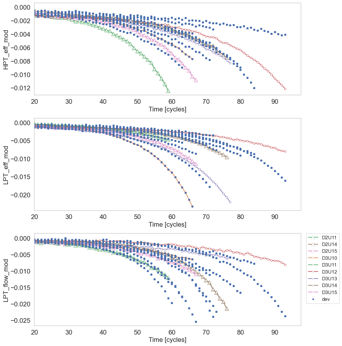
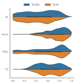
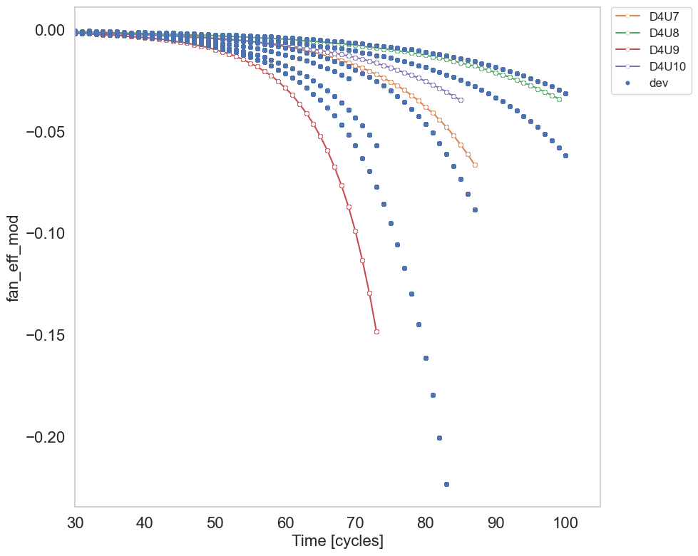
Such an OOD scenario can be observed for several units within data subsets D2, D3, and D4. In particular, units in data subsets D2, D3 are affected by a failure mode that involves the degradation of the low-pressure turbine (LPT) efficiency and flows in combination with the high-pressure turbine (HPT) efficiency, i.e., engine health parameters $\theta$. Figure 1 shows the degradation trajectories for development (blue), and the nine test units in D2 and D3 i.e., the evolution of the three causal factors of degradation $\theta$ = {HPT_eff_mod, LPT_flow_mod, LPT_Eff_mod} with time. We can observe that D2U11 (green triangles), D3U11 (green dots), and D3U12 (red dots) follow degradation trajectories that involve extrapolations outside the development data. As depicted in Figure 2 (right), a similar OOD behavior can be observed D4U09.

Figure 1: Evolution of the three causal factors of degradation $\theta$ = {HPT_eff_mod, LPT_flow_mod, LPT_Eff_mod} with time for development (blue), and the nine test units in D2 and D3. D2U11 (green triangles), D3U11 (green dots) and D3U12 (red dots) are OOD cases since they involve extrapolations of $\theta$ outside the development data.

It is worth mentioning that among the five considered datasets, D4 is a specially challenging dataset because of a couple of specificities (see Table 1): 1) it is the only dataset covering the degradation of the fan component, 2) it only contains flight classes 2 and 3. However, the distribution of the operating W parameters in the training and test sets are close enough (see the left plot in Figure 2).

Figure 2: (Left) Comparison between the train and test distributions of W parameters for units in D4. (Right) The degradation trajectory of Unit D4U9 (red) involves extrapolation on {fan_eff_mod}.

3.2.2 Feature selection and pre-processing

We selected the N-CMAPSS scenario descriptors and sensor measurements described in Table 2 as inputs, as well as the target RUL for our supervised learning approach. This makes an input size of $4+14=18$ values per time step.

Features	Description
$W$	4 scenario descriptors (flight conditions): altitude, Mach, TRA, T2
$X_{s}$	14 sensor measurements: physical fan speed, temp. at LPC outlet, …
Y	RUL label (remaining flight cycles)

Table 2: N-CMAPSS selected features.

We used a sliding window of length $30$ over the time series, so the resulting input size is $18\times 30$. To speed up computation, we downsampled sensor data to $0.1$ Hz by decimation, which results in windows of 5 minutes. All the input features were standardized to have zero mean and one standard deviation. We randomly split the sliding windows in the development set into 90% for training and 10% for validation. The number of units and window samples per dataset is shown in Table 3.

Dataset	# Units	# Samples	FC1	FC2	FC3
Train	33	$238\,182$	$0.10$	$0.27$	$0.62$
Validation	33	$26\,464$	$0.11$	$0.27$	$0.61$
Test	21	$144\,015$	$0.17$	$0.34$	$0.49$

Table 3: Number of engine units, sliding window samples and flight class ratios per dataset.

3.2.3 Piece-wise linear RUL degradation

The ideal true RUL is linearly decreasing over time, but in N-CMAPSS, engines follows a two-stage degradation trend. They stay healthy during the first cycles of operation. Then, their initial healthy state gradually deteriorates over the operation until reaching the end of life. Therefore, we could have used the piece-wise linear RUL target label function proposed in [67] for C-MAPSS to limit the maximum value of RUL to a constant value for all engines. However, setting a maximum RUL label for each engine is suboptimal, since each engine has a different life cycle. Instead, we corrected the labeling with the maximum RUL of each engine set to the RUL at the moment when a fault occurs and its actual deterioration begins, which is given by the parameter $h_{s}$ included in the N-CMAPSS auxiliary data.

3.3 Model architectures

3.3.1 Functional models

Functional models are deep neural network architectures used to build the probabilistic neural networks. After some preliminary testing with an adaptation of a fully-connected model (D3 [28]) and a convolutional one (C2P2 [29]) originally designed for C-MAPSS, we selected the Inception model [15] as it clearly outperformed the others.

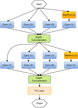
The Inception architecture (see Figure 3) achieved the second-best performance in the 2021 PHM Data Challenge to find the best deep learning architecture for N-CMAPSS. It uses several inception modules [14] to capture information lying at different scales through convolutions of different sizes applied to the same input. We used ReLU as activation function. The number of parameters of this model is $\sim 187k$, which will be doubled when turned into a BNN.

Figure 3: Inception model by DeVol et al. [15]

The functional models were implemented with PyTorch and PyTorch Lightning [68], and turned automatically into BNN with TyXe [69] based on Pyro [70].

3.3.2 Hyperparameter search

Hyperparameter tuning is particularly important for inference methods like MFVI suffering from hyperparameter sensitivity [46]. We implemented the hyperparameter search with Optuna [71] and performed 60 trials for each method. Models were trained with the Adam optimizer for only 20 epochs per trial to speed up the process. The hyperparameter search took about 5 days on 3 NVIDIA GeForce GTX 1080 Ti GPUs. We chose a sampling algorithm called TPESampler [16] combined with the median pruner algorithm available in Optuna.

For the BNN techniques, the search space was guided by the validation ELBO (20 Monte-Carlo (MC) samples of $q_{\theta}$ were used for validation) and included the exploration of the following parameters:

• Functional model pre-training with root-mean-square error (RMSE) (0 or 5 epochs)

• Number of $q_{\theta}$ MC samples for estimating training loss (1 or 2 samples)

• Gaussian prior scale (log-uniformly sampled between $10^{-2}$ and $0.5$)

• Gaussian $q_{\theta}$ scale (log-uniformly sampled between $10^{-4}$ and $10^{-2}$)

• The learning rate (log-uniformly sampled between $10^{-5}$ and $10^{-3}$)

• Batch size (100, 250, 500 or 1000 samples)

The pretraining of the functional model for a few epochs is a technique to help initialize the means of the Normal weight distributions. The best BNN hyperparameters found are listed in Table 4.

	LRT	FO	RAD
Training MC samples	1	2	1
Pre-train epochs	5	5	5
Prior scale	0.138793	0.198768	0.092516
$q_{\theta}$ scale	0.001351	0.000214	0.001241
Learning rate	0.000857	0.000948	0.000956
Batch size	100	100	100

Table 4: Hyperparameters for the variational BNN techniques.

The search space for the other techniques was guided by the validation NLL loss. For HNN, it included the batch size (same choices as with BNN) and the learning rate (log-uniformly sampled between $10^{-4}$ and $5^{-3}$). For MCD, we had, in addition, the number of MC samples (20, 50, 100) and dropout probability (uniformly sampled between $0.20$ and $0.85$). The final hyperparameters for these methods are listed in Table 5.

	HNN	MCD
MC samples	-	100
Dropout probability	-	0.241437
Learning rate	0.001574	0.000772
Batch size	250	100

Table 5: Hyperparameters for HNN and MCD.

3.3.3 Model training procedure

We performed 10 runs for HNN and 5 runs for the other methods by using different random seeds. The number of HNN runs was twice as many because we needed enough independently trained HNN models to build the DE. Indeed, there was no proper training involved for DE models. Instead, we generated 5 DE models as random combinations of 5 out of the 10 available HNN models. More than 5 models in the ensemble could have possibly resulted in better performance, but also in an unfair comparison with the other methods because of the huge difference in the number of parameters. We trained the models for a maximum number of 500 epochs using early stopping with patience 50 (HNN and MCD) and 20 (BNN). All models were trained with the best hyperparameters listed in Table 4 and Table 5. We minimized the validation ELBO for the BNNs, and the validation NLL for MCD and HNN.

Figure 4 plots train and validation ELBO and MSE losses for the BNN models. Training and validation curves are very close, especially in the case of the ELBO. Early stopping is activated earlier for RAD, whose validation ELBO converges faster and at a lower level than the LRT and FO ones. In terms of the validation MSE, however, the RAD curve is noisier and converges to a higher MSE value.

Figure 4: Losses during training and validation of the BNN methods.

Training and validation losses for the HNN and MCD methods are shown in Figure 5. We discarded 2 out of the 10 HNN runs because of significant anomalies in the training and validation curves. Otherwise, all runs produced very similar training and validation curves, with MCD converging slightly before HNN but at a higher loss level.

Figure 5: Losses during training and validation of HNN and MCD methods.

Table 6 provides some statistics showing big differences among the methods in terms of epochs and hours needed for each run. BNN models converge much faster than HNN and MCD, but the time taken to complete a run is significantly higher. Among the BNN techniques, the run time of RAD is the lowest and similar to the MCD one, whereas the one of FO is by far the highest of all methods. HNN is the fastest method and the one with the highest variance in the number of epochs. The latter is due to the two discarded runs which were stopped much earlier by the early stopping mechanism.

	Epochs	Time (h)
RAD	63.0 $\pm$ 15.2	6.8 $\pm$ 1.2
LRT	80.6 $\pm$ 19.6	8.7 $\pm$ 1.6
FO	116.4 $\pm$ 13.4	20.6 $\pm$ 1.8
HNN	177.5 $\pm$ 107.2	1.4 $\pm$ 0.7
MCD	241.0 $\pm$ 52.5	6.2 $\pm$ 0.9

Table 6: Number of epochs needed for a run to converge to the lowest validation loss and the number of hours taken for a run to finish with early stopping. Rows are sorted by the average number of epochs.

3.4 Evaluation metrics

We evaluated model accuracy with mean absolute error (MAE), root-mean-square error (RMSE) and NLL. MAE is less sensitive to outliers than RMSE. In fact, RMSE provides a measure of the worst-case accuracy. NLL is a proper scoring rule [17] assessing both the predictive accuracy of a model and the quality of its UQ estimate [72]. However, NLL can over-emphasize tail probabilities [13] and favors models that tend to be under-confident rather than over-confident [73]). We further assessed predictive uncertainty by measuring calibration and sharpness [74] with the tools provided in the Uncertainty Toolbox [75].

Calibration can be visualized with a calibration curve, which ‘displays the true frequency of points in each interval relative to the predicted fraction of points in that interval’ [74]. Thus, for $m$ confidence levels $0\leq p_{1}<p_{2}<\ldots<p_{m}\leq 1$ and a test set $\mathcal{T}=\{x_{t},y_{t}\}_{t=1}^{T}$, we can compute the empirical frequency for each threshold $p_{j}$ as:

$$\hat{p}_{j}=\frac{|\{y_{t}\mid F_{t}(y_{t})\leq p_{j},t=1,\ldots,T\}|}{T}$$

where $F_{t}(y_{t}\mid\hat{\mu}(x_{t}),\hat{\sigma}^{2}(x_{t}))=\frac{1}{2}\left[1+\mathrm{erf}\left(\frac{y_{t}-\hat{\mu}(x_{t})}{\hat{\sigma}^{2}(x_{t}){\sqrt{2}}}\right)\right]$ is the Gaussian CDF. The calibration curve is built from $\{(p_{j},\hat{p}_{j})\}_{j=1}^{m}$ and the root mean square calibration error (RMSCE) is computed as:

$$\mathrm{RMSCE}(F_{1},y_{1},\ldots,F_{T},y_{T})=\sqrt{\frac{1}{m}\sum_{j=1}^{m}(p_{j}-\hat{p}_{j})^{2}}$$ (6)

Well-calibrated models can still have large uncertainty estimates, which are less informative than smaller ones. We assess this aspect with the sharpness score [74], which is simply the average of the predicted variances:

$$\mathrm{Sharp}(F_{1},\ldots,F_{T})=\sqrt{\frac{1}{T}\sum_{t=1}^{T}\hat{\sigma}^{2}(x_{t})}$$ (7)

Please note that unlike in [74], we added the square root as suggested in [72] to give sharpness the same units as the predictions.

3.5 Uncertainty decomposition

We assessed for the different methods the possibility of separating the epistemic and aleatoric uncertainty from the total predictive uncertainty. In VI, we can derive this decomposition from the Bayesian Model Average of the variational approximation by adapting the method in [76]. The posterior predictive distribution is defined as:

$$p(y^{*}|x^{*},D)=\int_{\Omega}p(y^{*}|x^{*},\omega)p(\omega|D)d\omega\approx\int_{\Omega}p(y^{*}|x^{*},\omega)q_{\theta}(\omega)d\omega$$

We can then use it in the next equations

$$\mathop{\mathbb{E}\left[y^{*}\right]}_{p(y^{*}|x^{*},D)} =\int y^{*}p(y^{*}|x^{*},D)dy^{*}$$

$$=\int_{\Omega}q_{\theta}(\omega)\int y^{*}p(y^{*}|x^{*},\omega)\ dy^{*}d\omega$$

$$=\int_{\Omega}q_{\theta}(\omega)\mathop{\mathbb{E}\left[y^{*}\right]}_{p(y^{*}|x^{*},\omega)}d\omega$$

$$=\mathop{\mathbb{E}}_{\omega\sim q_{\theta}}\left[\mathop{\mathbb{E}\left[y^{*}\right]}_{p(y^{*}|x^{*},\omega)}\right]$$

In the same manner,

$$\mathop{\mathbb{E}\left[(y^{*})^{2}\right]}_{p(y^{*}|x^{*},D)} =\int_{\Omega}q_{\theta}(\omega)\int y^{*2}p(y^{*}|x^{*},\omega)\ dy^{*}d\omega$$

$$=\int_{\Omega}q_{\theta}(\omega)\mathop{\mathbb{E}\left[y^{*2}\right]}_{p(y^{*}|x^{*},\omega)}d\omega$$

$$=\int_{\Omega}q_{\theta}(\omega)\left(\mathop{\text{Var}}_{p(y^{*}|x^{*},\omega)}(y^{*})+\mathop{\mathbb{E}\left[y^{*}\right]^{2}}_{p(y^{*}|x^{*},\omega)}\right)d\omega$$

To compute the total variance

$$\mathop{\text{Var}}_{p(y^{*}|x^{*},D)}(y^{*}) =\mathop{\mathbb{E}\left[(y^{*})^{2}\right]}_{p(y^{*}|x^{*},D)}-\left(\mathop{\mathbb{E}\left[(y^{*})\right]}_{p(y^{*}|x^{*},D)}\right)^{2}$$

$$=\int_{\Omega}q_{\theta}(\omega)\left(\mathop{\text{Var}}_{p(y^{*}|x^{*},\omega)}(y^{*})+\mathop{\mathbb{E}\left[y^{*}\right]^{2}}_{p(y^{*}|x^{*},\omega)}\right)d\omega\ -\left(\int_{\Omega}q_{\theta}(\omega)\mathop{\mathbb{E}\left[y^{*}\right]}_{p(y^{*}|x^{*},\omega)}d\omega\right)^{2}$$

$$=\mathop{\mathbb{E}}_{\omega\sim q_{\theta}(\omega)}\left[\mathop{\text{Var}}_{p(y^{*}|x^{*},\omega)}(y^{*})\right]+\int_{\Omega}q_{\theta}(\omega)\mathop{\mathbb{E}\left[y^{*}\right]^{2}}_{p(y^{*}|x^{*},\omega)}d\omega-\left(\int_{\Omega}q_{\theta}(\omega)\mathop{\mathbb{E}\left[y^{*}\right]}_{p(y^{*}|x^{*},\omega)}d\omega\right)^{2}$$

$$=\mathop{\mathbb{E}}_{\omega\sim q_{\theta}(\omega)}\left[\mathop{\text{Var}}_{p(y^{*}|x^{*},\omega)}(y^{*})\right]+\mathop{\text{Var}}_{\omega\sim q_{\theta}(\omega)}\left[\mathop{\mathbb{E}\left[y^{*}\right]}_{p(y^{*}|x^{*},\omega)}\right]$$

Which is the analytical formula for

$$\mathop{\text{Var}}_{p(y^{*}|x^{*},D)}(y^{*})=\mathop{\text{Var}}_{\omega\sim q_{\theta}(\omega)}\left(\hat{\mu}\right)+\mathop{\mathbb{E}\left[\hat{\sigma}^{2}\right]}_{\omega\sim q_{\theta}(\omega)}$$ (8)

For a BNN or with MCD, the total predictive variance for outputs $\hat{\mu}$ and $\hat{\sigma}$ is computed by Monte-Carlo. Let vectors $\hat{\mu}=(\hat{\mu}_{1},...,\hat{\mu}_{n})$ and $\hat{\sigma}=(\hat{\sigma}_{1},...,\hat{\sigma}_{n})$ be the results of $n$ forward passes in the BNN with different weight samplings. Then, the total uncertainty $\hat{\sigma}_{\text{tot}}^{2}$ is defined as:

$$\hat{\sigma}_{\text{tot}}^{2}(x)=\underbrace{\frac{1}{N}\sum_{i=1}^{N}\hat{\mu}_{i}(x)^{2}-\left(\frac{1}{N}\sum_{i=1}^{N}\hat{\mu}_{i}(x)\right)^{2}}_{\text{epistemic part}}+\underbrace{\frac{1}{N}\sum_{i=1}^{N}\hat{\sigma}_{i}(x)^{2}}_{\text{aleatoric part}}$$ (9)

Concerning DE, the decomposition of predictive uncertainty is less straightforward. Recently, Egele et al. [77] proposed a method based on the law of total variance [77], where they randomly select $K$ models from a catalog to form the ensemble. However, they assume a great model diversity in the ensemble, which is far from being our case with only 5 identical models. Therefore, we have not implemented the separation of uncertainties for DE. In the case of HNN, the epistemic uncertainty is not modeled, so the separation of predictive uncertainty into aleatoric and epistemic makes no sense.

4 Results and discussions

4.1 Summary metrics

The performance of the methods in Section 3.1 is evaluated against the 21 units of the N-CMAPSS test set with the metrics specified in Section 3.4, and the hyperparameters listed in Table 4 and Table 5. The results aggregated over the runs are summarized in Table 7.

	MAE $\downarrow$	RMSE $\downarrow$	NLL $\downarrow$	RMSCE $\downarrow$	Sharp $\downarrow$
DE	6.277 $\pm$ 0.168	8.163 $\pm$ 0.136	2.372 $\pm$ 0.017	0.063 $\pm$ 0.018	10.676 $\pm$ 0.961
MCD	6.376 $\pm$ 0.143	8.466 $\pm$ 0.216	2.396 $\pm$ 0.024	0.071 $\pm$ 0.005	11.278 $\pm$ 0.424
HNN	6.203 $\pm$ 0.163	8.279 $\pm$ 0.181	2.516 $\pm$ 0.057	0.049 $\pm$ 0.015	8.733 $\pm$ 0.320
RAD	6.483 $\pm$ 0.102	8.619 $\pm$ 0.100	3.181 $\pm$ 0.533	0.051 $\pm$ 0.016	9.472 $\pm$ 0.494
LRT	6.403 $\pm$ 0.108	8.551 $\pm$ 0.122	4.553 $\pm$ 2.008	0.076 $\pm$ 0.017	9.031 $\pm$ 0.350
FO	6.158 $\pm$ 0.109	8.235 $\pm$ 0.113	5.007 $\pm$ 0.465	0.089 $\pm$ 0.012	8.581 $\pm$ 0.209

Table 7: Performance metrics on the test set for all the methods described in Section 3.1. The units of RMSE and sharpness are in flight cycles. NLL and RMSCE are unitless. Rows are sorted by increasing NLL, and smaller values are better ($\downarrow$).

In terms of NLL, which is the only metric accounting for both predictive accuracy and quality of uncertainty estimates, the performance of BNN models is worse than the one of frequentist alternatives. DE and MCD obtain the best NLL scores, but their largest sharpness can be a drawback for decision-making. In the case of BNN models, NLL variance across runs is orders of magnitude higher than in other methods, especially for the FO method. We can observe good NLL scores have a good correlation with the most conservative estimates of uncertainty, which is in line with the findings in [13, 73, 72]. Therefore, if we rank models on NLL alone, we will clearly favor those yielding under-confident rather than over-confident uncertainty estimates.

FO is the method with the best sharpness but at the cost of the worst calibration leading to the poorest RMSCE and NLL. On the contrary, HNN and RAD calibration are the best. In spite of its relative simplicity, HNN outperforms BNNs in terms of NLL, and offers the best calibration along with a competitive sharpness. As for accuracy, no method clearly outperforms the others when looking at the metrics in Table 7, and differences in the scores are sometimes close and statistically insignificant. For instance, FO, HNN, and DE have got the top accuracy, but the other methods fall close behind in terms of MAE and RMSE.

4.2 Metrics per dataset

The performance per dataset averaged over the results of all methods is summarized in Table 8. Although aggregated performance per dataset is not useful for method ranking, it can help focus method performance analysis on the most challenging data subsets. In that sense, D3 deserves special attention as it has the highest NLL score. Also, a large NLL variance points to substantial differences depending on the model. On the other hand, D4 has the biggest MAE and RMSE scores, along with a large uncertainty (sharpness) in the predictions. However, a relatively moderate NLL and the lowest RMSCE indicates a good calibration of its predictive uncertainty. Finally, D1 and D5 seem overall less problematic for the models, whereas model predictions for D2 together with D3 are the worst calibrated.

	MAE $\downarrow$	RMSE $\downarrow$	NLL $\downarrow$	RMSCE $\downarrow$	Sharp $\downarrow$
D2	6.129 $\pm$ 0.470	8.193 $\pm$ 0.668	2.848 $\pm$ 1.121	0.138 $\pm$ 0.057	7.323 $\pm$ 1.032
D1	4.935 $\pm$ 0.281	6.522 $\pm$ 0.305	2.856 $\pm$ 1.198	0.061 $\pm$ 0.039	8.812 $\pm$ 1.066
D4	9.126 $\pm$ 0.683	11.366 $\pm$ 0.597	2.944 $\pm$ 0.169	0.034 $\pm$ 0.018	12.893 $\pm$ 1.382
D5	4.354 $\pm$ 0.312	5.769 $\pm$ 0.310	3.013 $\pm$ 1.058	0.076 $\pm$ 0.061	8.862 $\pm$ 1.279
D3	6.063 $\pm$ 0.208	7.815 $\pm$ 0.343	4.32 $\pm$ 3.008	0.132 $\pm$ 0.065	7.729 $\pm$ 1.046

Table 8: Performance metrics aggregated per dataset in the test set. Rows are sorted by increasing NLL and smaller values are better ($\downarrow$). The worst scores are highlighted in bold.

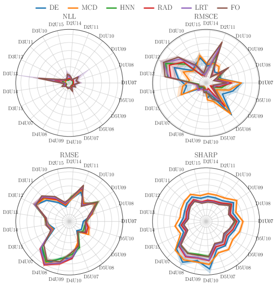
Figure 6 provides an overview of method metrics per unit in the test set. The goal is to spot where method performance diverges the most and which units are the most challenging for each method. For instance, we can see that if D3 has the worst NLL score, this is greatly due to the single contribution of D3U13 and the BNN methods, especially LRT and FO. We can also observe FO is causing the large NLL variance. The significantly higher NLL score of this unit is consistent with its poor calibration (RMSCE) and indicates its sharpness (the lowest of all units) seems overly optimistic for the BNN. The overconfidence of these models with D3U13 could be explained by the confusing presence in the training set of a unit whose degradation may look similar, but it is actually different, for instance in terms of number of cycles (see Figure 1).

On the contrary, RMSE scores are quite homogeneous across the methods. Also, all agree that unit D4U08 is one of the hardest to predict accurately, whereas unit D5U08 is one of the easiest ones. In terms of accuracy, units D4U08, D4U09, D4U07, D3U12 and D2U11 present the highest RMSE scores.

Concerning the calibration, we can observe significant differences across the methods depending on the unit. For instance, RMSCE for the BNN and HNN models is relatively higher compared to the other methods in units D2U11, D3U11 and D3U12. However, for DE and MCD, D2U15, D3U14 and D3U15 calibration is much worse. As for the sharpness, method performance per unit is similar, with DE and MCD yielding systematically the most conservative scores.

Figure 6: Performance metrics aggregated per engine unit and method.

4.3 Metrics per flight class

As stated in [18], each engine unit is assumed to operate only one of the three flight classes, i.e. short (FC1), medium (FC2) and long-haul (FC3) flights. Table 3 shows the distribution of flight classes in the training, validation and test subsets. The distribution in the training set is highly unbalanced in favour of FC3 which represents 62% of the samples, followed by FC2 (27%) and FC1 (11%). The validation set distribution is very similar to the training set. The test set is a bit more balanced with FC3 representing 49%, FC2 34% and FC1 17%.

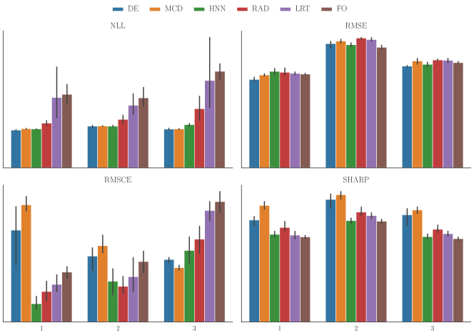
Therefore, we can expect this unbalanced training set to have a negative impact in the performance of FC1 units. Yet, we do not observe that when looking at Figure 7, which shows the method performance metrics across flight classes. In terms of accuracy, FC2 followed by FC3 are actually the classes with the worst scores. However, this is highly influenced by the contribution of D4, which is specific in terms of failure mode and has no FC1. When we removed D4, FC1 became one with the largest sharpness and the second-worst accuracy.

Other than that, the important fact to note is the difference in calibration performance across flight classes between DE and MCD and the BNN techniques. DE and MCD have a much worse calibration with FC1, whereas BNNs present a significantly higher RMSCE with FC3. However, the NLL plot tells a very different story, with DE and MCD yielding systematically better scores than the BNN models for all flight classes. The relative conservative sharpness and slightly better accuracy of DE and MCD translate into a surprisingly better NLL score than expected. This is an example on how the NLL score can be quite misleading by favoring the most conservative models.

Figure 7: Performance metrics aggregated per flight class and method.

4.4 Quality of predictive uncertainty

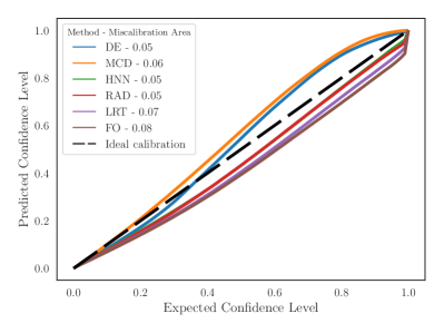
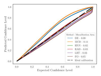
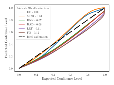
The calibration curves and the miscalibration area per method on the test units are displayed in the left plot in Figure 8. LRT and FO are the most overconfident (confident intervals too narrow). On the contrary, MCD and DE are under-confident (confident intervals too wide), especially from the mid-end of the system lifetime. FO has the highest miscalibration area, whereas RAD and HNN has the lowest ones, which is close to the ranking obtained with the RMSCE score.

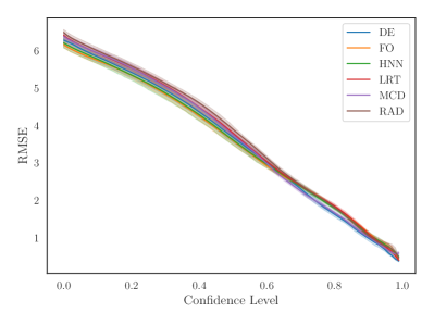
For decision-making, a highly desirable property is that we can trust a model when the confidence in the prediction is high so that we can use a back-up solution when it is not (e.g., demand for human intervention). To evaluate this capability, we can plot model accuracy as a function of the confidence in the predictions, as shown in the right plot in Figure 8. This plot allows us to evaluate the model only when its confidence is above a certain threshold, or equivalently when the predictive uncertainty or variance ($\sigma^{2}$) is below a certain threshold. The higher the model confidence (the lower the predictive uncertainty), the better RMSE should be. Indeed, this inverse trend is exactly what we observe for all the methods, without any significant difference among them.

Figure 8: (Left) Method uncertainty calibration curves (ideal: $y=x$) and miscalibration area. (Right) RMSE versus confidence. Higher confidence levels correspond with lower predictive uncertainty ($\sigma^{2}$). The desirable inverse trend between RMSE and confidence level is observed across all methods.

It is worth further exploring what happens with the calibration of flight classes FC1 and FC3, given the observed differences in RMSCE between DE and MCD on one side and the BNNs on the other. Figure 9 provides a comparison between the calibration of the two flight classes. HNN and BNN calibrations are excellent for FC1 units, whereas DE and MCD suffer from under-confidence. For FC3 units, HNN and BNNs are far overconfident, and DE and MCD calibrations are better than for FC1 units, especially in the case of MCD.

Figure 9: Calibration comparison between flight classes: FC1 units (left) and FC3 units (right).

Another way of measuring if a model knows what it knows concerns the generalization or robustness of the predictive uncertainty. This is usually evaluated in cases of domain shift between the train and the test set (OOD data). In OOD units, we expect high sharpness score or entropy  combined perhaps with low accuracy. However, these conditions do not necessarily occur only in OOD situations, whose confirmation requires analyzing the differences in the operating parameters and degradation profiles between the train and test datasets (see Section 3.2).

For instance, we see in Figure 6 that units with the largest sharpness are the ones in D4. We showed in Section 3.2 this is due to the fact that D4 is a challenging dataset because of its specificities. The right plot in Figure 10 shows D4 has also the worst accuracy and sharpness in the train set, which further supports the assumption that what happens with D4 as a whole cannot be simply explained in terms of distributional shift.

Figure 10: Metrics per dataset for the test (left) and training (right) sets. D4 RMSE and sharpness is already the worst in training set, suggesting large sharpness in the test set may not be only linked to OOD.

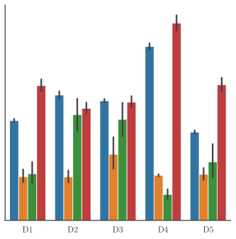
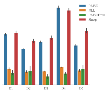
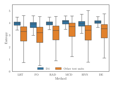
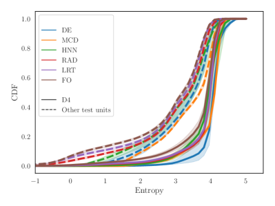
Indeed, this illustrates rather a case of robustness of predictive uncertainty to a dataset where degradation is genuinely harder to predict. All methods are robust in the sense their high RMSE is linked to large sharpness and good calibration (low RMSCE). We can better visualize what happens by comparing the entropy distributions of the D4 test units vs the rest of test units. We see in Figure 11 all methods exhibit higher entropy levels for the D4 units. The degree of separation in the entropy distributions depends on the method, i.e., it is less evident with MCD and HNN than with RAD, LRT and DE.

Figure 11: Entropy comparison between D4 test units and the rest of test units. All methods estimate higher uncertainty levels for D4 units.

Figure 12: Entropy comparison between in-distribution (ID) and out-of-distribution(OOD) test units (D2U11, D3U11 and D3U12). All methods estimate lower levels of entropy for OOD units due to bad calibration (overconfidence).

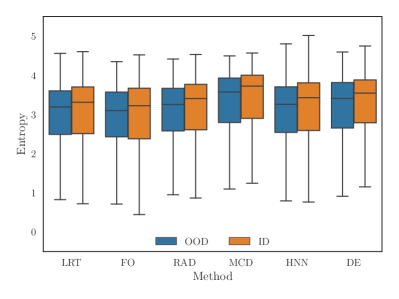
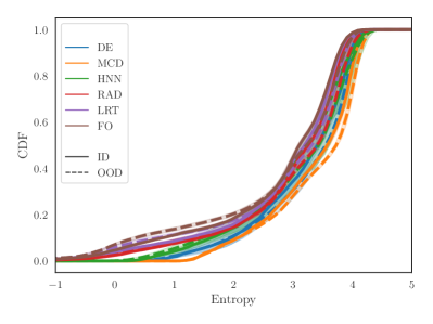
In Section 3.2, we identified D2U11, D3U11 and D3U12 as potential OOD cases because of their degradation profiles being significantly different from the rest. However, Figure 6 shows that sharpness is not as high as it should be for these OOD units. What is actually high instead is both their RMSE and RMSCE, the latter pointing to calibrations being among the worst ones, especially for the BNNs and HNN models. Figure 12 allows us to compare the entropy distributions of ID and OOD units. Unfortunately, all methods exhibit indeed an entropy which is slightly lower for the OOD units, which is due to overconfidence. Thus, robustness of the methods to OOD data is severely compromised by bad calibration associated with poor accuracy. We think these results are significant and should be further investigated in future work.

4.5 Method performance over the system lifetime

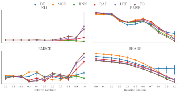
Reliability of RUL predictions is obviously most needed when a system reaches the end of life, where wrong predictions have a higher economic and safety cost. Figure 13 shows the evolution of the metrics aggregated over all the test units. The downward trend in RMSE and sharpness achieved by all methods is reassuring in the sense predictions become more accurate and certain by the end, especially in the case of HNN and BNNs. However, we can observe a change from a downtrend to an uptrend in the DE sharpness at around 70% of the system lifetime. More worrying is the surge at the end in the RMSCE and NLL scores of the BNN models.

Figure 13: Method performance evolution over the system lifetime.

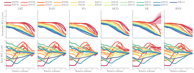
The evolution of predictive uncertainty and prediction error (see Figure 14) follows consequently a downward trend as well for most of the units. Again, we see how the uncertainty and predictive errors are higher for D4 units, especially for D4U08 and D4U09. For these units, the pattern of evolution differs, and a peak in error can be observed in all methods at around 60% of the system lifetime. In the case of DE, the surge on the uncertainty at the later cycles towards the end of life is to be mostly attributed to D4U08 and D4U09 units.

Figure 14: Evolution of predictive uncertainty and prediction error per method on the test set units.

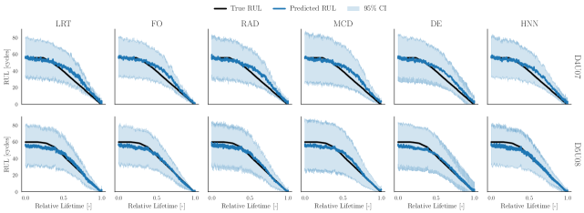
As an illustrative example, Figure 15 compares the RUL predictions for one of the difficult units (D4U07) against one of the easiest ones (D5U08). The blue line (predicted RUL) follows the black line (true RUL) more or less accurately, depending on the unit and the method. In all cases, predictive uncertainty is reduced when approaching the end of life, as it is shown with the 95% confidence interval in light blue.

Figure 15: RUL estimations for units D4U07 and D5U08.

4.6 Epistemic and aleatoric UQ

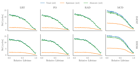
Figure 16 provides a comparison of the decomposition of the predictive uncertainty into aleatoric and epistemic uncertainty as per Equation 9 for D4U07 and D5U08. As we are using standard deviations instead of variances, the sum of the aleatoric (green) and epistemic (orange) uncertainties is not equal to the total uncertainty (blue). The dominance of the aleatoric uncertainty over the epistemic one is very clear, especially for the BNN. The resulting decomposition is slightly dependent on the method, but very similar for the three BNN techniques. Differences are minor in the decomposition between an easy or a difficult-to-predict unit. We see a clear decreasing trend in the aleatoric uncertainty over the time, whereas the epistemic one remains relatively more constant, which is in agreement with the results in [55]. For aleatoric uncertainty, the explanation lies in the accumulative nature of noise over the lifetime of the system. This is not the case with the epistemic uncertainty, which only depends on the availability of training data covering the system’s lifetime.

Figure 16: Break-down of predictive uncertainty into epistemic and aleatoric uncertainty for units D4U07 and D5U08.

5 Conclusion

Following a literature review, we examined a set of UQ methods for deep learning RUL estimation, including recent variational BNN methods for gradient variance reduction as well as alternatives like MCD, DE and a frequentist HNN. We have evaluated the performance of these methods with the recent N-CMAPSS dataset in terms of prediction accuracy and quality of the predictive uncertainty. All the considered methods scale relatively well with the size of N-CMAPSS and provide sensible uncertainty estimates and accurate RUL predictions in most of the test cases. However, we have not found any of the methods to be particularly robust to OOD cases, but BNN and HNN methods seem to suffer even more in OOD from low accuracy associated with overconfidence.

Comprehensive evaluation of the methods based on a set of UQ metrics is not straightforward. There exists a trade-off between them, e.g., between calibration and sharpness. Even scoring rules like NLL, which consider both calibration and sharpness altogether, seems biased towards under-confident models. In other words, it is not possible to rank the methods based on a single metric, the existence of which is an open research problem. The evaluation is also challenging because method performance depends on the subset of data considered (e.g., unit, flight class).

In spite of their complexity, we have not found BNN models to clearly outperform the simpler alternatives. Indeed, results show that HNN models can be a competitive and balanced alternative. HNN models are lighter, as well as much faster and more straightforward to train than BNN models. DE and MCD suffer from conservative uncertainty estimates, which may not be informative enough for decision-making. If we need to break down epistemic and aleatoric uncertainties (e.g. for active learning), MCD and RAD are probably the best choices to consider.

Based on the relatively good performance achieved by HNN, it would be interesting to include in our benchmark other non-Bayesian techniques to improve the vanilla HNN we used. For instance, deep evidential regression [78] or the improvements suggested in [9, 8] would be worth considering. Another aspect to evaluate we excluded from the benchmark is the influence of likelihood functions other than the basic Gaussian, such as skewed Gaussian, the Weibull, or Logistic ones.

In future work, we think the robustness of the methods to OOD situations should deserve a deeper assessment. We could, for instance, exclude a flight class from the training set or use combinations of training and test units with different degrees of distributional shifts. Safety aspects related to the reliability of the RUL estimates towards the end of the system lifetime should be further investigated as well. Finally, the benchmark could be extended to include deep Gaussian process models as well, since the work in [58] is based only on the D2 subset of N-CMAPSS making comparisons with our results difficult.

References

- Lee et al. [2014] Jay Lee, Fangji Wu, Wenyu Zhao, Masoud Ghaffari, Linxia Liao, and David Siegel. Prognostics and health management design for rotary machinery systems—reviews, methodology and applications. Mechanical Systems and Signal Processing, 42(1):314–334, 2014. ISSN 0888-3270. doi: https://doi.org/10.1016/j.ymssp.2013.06.004. URL https://www.sciencedirect.com/science/article/pii/S0888327013002860.
- Der Kiureghian and Ditlevsen [2009] Armen Der Kiureghian and Ove Ditlevsen. Aleatory or epistemic? does it matter? Structural safety, 31(2):105–112, 2009.
- Kendall and Gal [2017] Alex Kendall and Yarin Gal. What uncertainties do we need in bayesian deep learning for computer vision? Advances in neural information processing systems, 30, 2017.
- Gal et al. [2017] Yarin Gal, Riashat Islam, and Zoubin Ghahramani. Deep bayesian active learning with image data. In International Conference on Machine Learning, pages 1183–1192. PMLR, 2017.
- Zhu et al. [2022] Rong Zhu, Yuan Chen, Weiwen Peng, and Zhi-Sheng Ye. Bayesian deep-learning for rul prediction: An active learning perspective. Reliability Engineering & System Safety, 228:108758, 2022. ISSN 0951-8320. doi: https://doi.org/10.1016/j.ress.2022.108758. URL https://www.sciencedirect.com/science/article/pii/S0951832022003817.
- Amodei et al. [2016] Dario Amodei, Chris Olah, Jacob Steinhardt, Paul Christiano, John Schulman, and Dan Mané. Concrete problems in ai safety. arXiv preprint arXiv:1606.06565, 2016.
- Guo et al. [2017] Chuan Guo, Geoff Pleiss, Yu Sun, and Kilian Q Weinberger. On calibration of modern neural networks. In International conference on machine learning, pages 1321–1330. PMLR, 2017.
- Skafte et al. [2019] Nicki Skafte, Martin Jørgensen, and Søren Hauberg. Reliable training and estimation of variance networks. Advances in Neural Information Processing Systems, 32, 2019.
- Seitzer et al. [2022] Maximilian Seitzer, Arash Tavakoli, Dimitrije Antic, and Georg Martius. On the pitfalls of heteroscedastic uncertainty estimation with probabilistic neural networks. arXiv preprint arXiv:2203.09168, 2022.
- Blundell et al. [2015] Charles Blundell, Julien Cornebise, Koray Kavukcuoglu, and Daan Wierstra. Weight uncertainty in neural network. In International conference on machine learning, pages 1613–1622. PMLR, 2015.
- Gal and Ghahramani [2016] Yarin Gal and Zoubin Ghahramani. Dropout as a Bayesian Approximation: Representing Model Uncertainty in Deep Learning. arXiv:1506.02142 [cs, stat], October 2016. URL http://arxiv.org/abs/1506.02142.
- Lakshminarayanan et al. [2017] Balaji Lakshminarayanan, Alexander Pritzel, and Charles Blundell. Simple and Scalable Predictive Uncertainty Estimation using Deep Ensembles. arXiv:1612.01474 [cs, stat], November 2017. URL http://arxiv.org/abs/1612.01474.
- Ovadia et al. [2019] Yaniv Ovadia, Emily Fertig, Jie Ren, Zachary Nado, David Sculley, Sebastian Nowozin, Joshua Dillon, Balaji Lakshminarayanan, and Jasper Snoek. Can you trust your model’s uncertainty? evaluating predictive uncertainty under dataset shift. Advances in neural information processing systems, 32, 2019.
- Szegedy et al. [2015] Christian Szegedy, Wei Liu, Yangqing Jia, Pierre Sermanet, Scott Reed, Dragomir Anguelov, Dumitru Erhan, Vincent Vanhoucke, and Andrew Rabinovich. Going deeper with convolutions. In Proceedings of the IEEE conference on computer vision and pattern recognition, pages 1–9, 2015.
- DeVol et al. [2021] Nathaniel DeVol, Christopher Saldana, and Katherine Fu. Inception based deep convolutional neural network for remaining useful life estimation of turbofan engines. In Annual Conference of the PHM Society, volume 13, 2021.
- Bergstra et al. [2011] James Bergstra, Rémi Bardenet, Yoshua Bengio, and Balázs Kégl. Algorithms for hyper-parameter optimization. Advances in neural information processing systems, 24, 2011.
- Gneiting and Raftery [2007] Tilmann Gneiting and Adrian E Raftery. Strictly proper scoring rules, prediction, and estimation. Journal of the American statistical Association, 102(477):359–378, 2007.
- Arias Chao et al. [2021] Manuel Arias Chao, Chetan Kulkarni, Kai Goebel, and Olga Fink. Aircraft engine run-to-failure dataset under real flight conditions for prognostics and diagnostics. Data, 6(1):5, 2021.
- Dawid [1982] A Philip Dawid. The well-calibrated bayesian. Journal of the American Statistical Association, 77(379):605–610, 1982.
- DeGroot and Fienberg [1983] Morris H DeGroot and Stephen E Fienberg. The comparison and evaluation of forecasters. Journal of the Royal Statistical Society: Series D (The Statistician), 32(1-2):12–22, 1983.
- Fink et al. [2020] Olga Fink, Qin Wang, Markus Svensen, Pierre Dersin, Wan-Jui Lee, and Melanie Ducoffe. Potential, challenges and future directions for deep learning in prognostics and health management applications. Engineering Applications of Artificial Intelligence, 92:103678, 2020.
- Biggio and Kastanis [2020] Luca Biggio and Iason Kastanis. Prognostics and health management of industrial assets: Current progress and road ahead. Frontiers in Artificial Intelligence, 3:578613, 2020.
- Li et al. [2018] Xiang Li, Qian Ding, and Jian-Qiao Sun. Remaining useful life estimation in prognostics using deep convolution neural networks. Reliability Engineering & System Safety, 172:1–11, 2018.
- Ren et al. [2018] Lei Ren, Yaqiang Sun, Hao Wang, and Lin Zhang. Prediction of bearing remaining useful life with deep convolution neural network. IEEE access, 6:13041–13049, 2018.
- Wu et al. [2018] Yuting Wu, Mei Yuan, Shaopeng Dong, Li Lin, and Yingqi Liu. Remaining useful life estimation of engineered systems using vanilla lstm neural networks. Neurocomputing, 275:167–179, 2018.
- Chen et al. [2019] Jinglong Chen, Hongjie Jing, Yuanhong Chang, and Qian Liu. Gated recurrent unit based recurrent neural network for remaining useful life prediction of nonlinear deterioration process. Reliability Engineering & System Safety, 185:372–382, 2019.
- Wu et al. [2020] Jun Wu, Kui Hu, Yiwei Cheng, Haiping Zhu, Xinyu Shao, and Yuanhang Wang. Data-driven remaining useful life prediction via multiple sensor signals and deep long short-term memory neural network. ISA transactions, 97:241–250, 2020.
- Benker et al. [2021] Maximilian Benker, Lukas Furtner, Thomas Semm, and Michael F Zaeh. Utilizing uncertainty information in remaining useful life estimation via bayesian neural networks and hamiltonian monte carlo. Journal of Manufacturing Systems, 61:799–807, 2021.
- Sateesh Babu et al. [2016] Giduthuri Sateesh Babu, Peilin Zhao, and Xiao-Li Li. Deep convolutional neural network based regression approach for estimation of remaining useful life. In International conference on database systems for advanced applications, pages 214–228. Springer, 2016.
- Lövberg [2021] Andreas Lövberg. Remaining useful life prediction of aircraft engines with variable length input sequences. In Proceedings of the Annual Conference of the PHM Society, 2021.
- Ganin et al. [2016] Yaroslav Ganin, Evgeniya Ustinova, Hana Ajakan, Pascal Germain, Hugo Larochelle, François Laviolette, Mario Marchand, and Victor Lempitsky. Domain-adversarial training of neural networks. The journal of machine learning research, 17(1):2096–2030, 2016.
- da Costa et al. [2020] Paulo Roberto de Oliveira da Costa, Alp Akçay, Yingqian Zhang, and Uzay Kaymak. Remaining useful lifetime prediction via deep domain adaptation. Reliability Engineering & System Safety, 195:106682, 2020.
- Sabour et al. [2017] Sara Sabour, Nicholas Frosst, and Geoffrey E Hinton. Dynamic routing between capsules. Advances in neural information processing systems, 30, 2017.
- Ruiz-Tagle Palazuelos et al. [2020] Andres Ruiz-Tagle Palazuelos, Enrique López Droguett, and Rodrigo Pascual. A novel deep capsule neural network for remaining useful life estimation. Proceedings of the Institution of Mechanical Engineers, Part O: Journal of Risk and Reliability, 234(1):151–167, 2020.
- Gawlikowski et al. [2021] Jakob Gawlikowski, Cedrique Rovile Njieutcheu Tassi, Mohsin Ali, Jongseok Lee, Matthias Humt, Jianxiang Feng, Anna Kruspe, Rudolph Triebel, Peter Jung, Ribana Roscher, et al. A survey of uncertainty in deep neural networks. arXiv preprint arXiv:2107.03342, 2021.
- Abdar et al. [2021] Moloud Abdar, Farhad Pourpanah, Sadiq Hussain, Dana Rezazadegan, Li Liu, Mohammad Ghavamzadeh, Paul Fieguth, Xiaochun Cao, Abbas Khosravi, U Rajendra Acharya, et al. A review of uncertainty quantification in deep learning: Techniques, applications and challenges. Information Fusion, 76:243–297, 2021.
- Nix and Weigend [1994] David A Nix and Andreas S Weigend. Estimating the mean and variance of the target probability distribution. In Proceedings of 1994 ieee international conference on neural networks (ICNN’94), volume 1, pages 55–60. IEEE, 1994.
- Bishop [1994] Christopher M. Bishop. Mixture density networks. 1994. URL https://publications.aston.ac.uk/id/eprint/373/.
- MacKay [1992] David JC MacKay. A practical bayesian framework for backpropagation networks. Neural computation, 4(3):448–472, 1992.
- Neal et al. [2011] Radford M Neal et al. Mcmc using hamiltonian dynamics. Handbook of markov chain monte carlo, 2(11):2, 2011.
- Ritter et al. [2018] Hippolyt Ritter, Aleksandar Botev, and David Barber. A scalable laplace approximation for neural networks. In 6th International Conference on Learning Representations, ICLR 2018-Conference Track Proceedings, volume 6. International Conference on Representation Learning, 2018.
- Hernández-Lobato and Adams [2015] José Miguel Hernández-Lobato and Ryan Adams. Probabilistic backpropagation for scalable learning of bayesian neural networks. In International conference on machine learning, pages 1861–1869. PMLR, 2015.
- Graves [2011] Alex Graves. Practical variational inference for neural networks. Advances in neural information processing systems, 24, 2011.
- Kingma et al. [2015] Durk P Kingma, Tim Salimans, and Max Welling. Variational dropout and the local reparameterization trick. Advances in neural information processing systems, 28, 2015.
- Wen et al. [2018] Yeming Wen, Paul Vicol, Jimmy Ba, Dustin Tran, and Roger Grosse. Flipout: Efficient pseudo-independent weight perturbations on mini-batches. arXiv preprint arXiv:1803.04386, 2018.
- Farquhar et al. [2020] Sebastian Farquhar, Michael A Osborne, and Yarin Gal. Radial bayesian neural networks: Beyond discrete support in large-scale bayesian deep learning. In International Conference on Artificial Intelligence and Statistics, pages 1352–1362. PMLR, 2020.
- Tomczak et al. [2020] Marcin Tomczak, Siddharth Swaroop, and Richard Turner. Efficient low rank gaussian variational inference for neural networks. Advances in Neural Information Processing Systems, 33:4610–4622, 2020.
- Kefalas et al. [2022] Marios Kefalas, Bas van Stein, Mitra Baratchi, Asteris Apostolidis, and Thomas Back. An End-to-End Pipeline for Uncertainty Quantification and Remaining Useful Life Estimation: An Application on Aircraft Engines. In Proceedings of the IEEE conference on computer vision and pattern recognition, page 16, June 2022.
- Caceres et al. [2021] Jose Caceres, Danilo Gonzalez, Taotao Zhou, and Enrique Lopez Droguett. A probabilistic bayesian recurrent neural network for remaining useful life prognostics considering epistemic and aleatory uncertainties. Structural Control and Health Monitoring, 28(10):e2811, 2021.
- Saxena et al. [2008] Abhinav Saxena, Kai Goebel, Don Simon, and Neil Eklund. Damage propagation modeling for aircraft engine run-to-failure simulation. In 2008 international conference on prognostics and health management, pages 1–9. IEEE, 2008.
- Peng et al. [2019] Weiwen Peng, Zhi-Sheng Ye, and Nan Chen. Bayesian deep-learning-based health prognostics toward prognostics uncertainty. IEEE Transactions on Industrial Electronics, 67(3):2283–2293, 2019.
- Kraus and Feuerriegel [2019] Mathias Kraus and Stefan Feuerriegel. Forecasting remaining useful life: Interpretable deep learning approach via variational bayesian inferences. Decision Support Systems, 125:113100, 2019.
- Wang et al. [2020] Biao Wang, Yaguo Lei, Tao Yan, Naipeng Li, and Liang Guo. Recurrent convolutional neural network: A new framework for remaining useful life prediction of machinery. Neurocomputing, 379:117–129, 2020.
- Zhao et al. [2020] Zhibin Zhao, Jingyao Wu, David Wong, Chuang Sun, and Ruqiang Yan. Probabilistic remaining useful life prediction based on deep convolutional neural network. 2020.
- Li et al. [2020] Gaoyang Li, Li Yang, Chi-Guhn Lee, Xiaohua Wang, and Mingzhe Rong. A bayesian deep learning rul framework integrating epistemic and aleatoric uncertainties. IEEE Transactions on Industrial Electronics, 68(9):8829–8841, 2020.
- Huang et al. [2020] Dengshan Huang, Rui Bai, Shuai Zhao, Pengfei Wen, Shengyue Wang, and Shaowei Chen. Bayesian neural network based method of remaining useful life prediction and uncertainty quantification for aircraft engine. In 2020 IEEE International Conference on Prognostics and Health Management (ICPHM), pages 1–8. IEEE, 2020.
- Deng et al. [2020] Yingjun Deng, Alessandro Di Bucchianico, and Mykola Pechenizkiy. Controlling the accuracy and uncertainty trade-off in rul prediction with a surrogate wiener propagation model. Reliability Engineering & System Safety, 196:106727, 2020.
- Biggio et al. [2021] Luca Biggio, Alexander Wieland, Manuel Arias Chao, Iason Kastanis, and Olga Fink. Uncertainty-aware prognosis via deep gaussian process. IEEE Access, 9:123517–123527, 2021.
- Hinton and Van Camp [1993] Geoffrey E Hinton and Drew Van Camp. Keeping the neural networks simple by minimizing the description length of the weights. In Proceedings of the sixth annual conference on Computational learning theory, pages 5–13, 1993.
- Jaakkola and Jordan [2000] Tommi S Jaakkola and Michael I Jordan. Bayesian parameter estimation via variational methods. Statistics and Computing, 10(1):25–37, 2000.
- Neal and Hinton [1998] Radford M Neal and Geoffrey E Hinton. A view of the em algorithm that justifies incremental, sparse, and other variants. In Learning in graphical models, pages 355–368. Springer, 1998.
- Silvestro and Andermann [2020] Daniele Silvestro and Tobias Andermann. Prior choice affects ability of Bayesian neural networks to identify unknowns. arXiv:2005.04987 [cs, stat], May 2020. URL http://arxiv.org/abs/2005.04987. arXiv: 2005.04987.
- Nalisnick [2018] Eric Thomas Nalisnick. On Priors for Bayesian Neural Networks. PhD thesis, UC Irvine, 2018. URL https://escholarship.org/uc/item/1jq6z904.
- Wilson and Izmailov [2020] Andrew Gordon Wilson and Pavel Izmailov. Bayesian deep learning and a probabilistic perspective of generalization. CoRR, abs/2002.08791, 2020. URL https://arxiv.org/abs/2002.08791.
- Bishop and Nasrabadi [2006] Christopher M Bishop and Nasser M Nasrabadi. Pattern recognition and machine learning, volume 4. Springer, 2006.
- Srivastava et al. [2014] Nitish Srivastava, Geoffrey Hinton, Alex Krizhevsky, Ilya Sutskever, and Ruslan Salakhutdinov. Dropout: a simple way to prevent neural networks from overfitting. The journal of machine learning research, 15(1):1929–1958, 2014.
- Zhang et al. [2018] Jianjing Zhang, Peng Wang, Ruqiang Yan, and Robert X Gao. Long short-term memory for machine remaining life prediction. Journal of manufacturing systems, 48:78–86, 2018.
- Falcon and The PyTorch Lightning team [2019] William Falcon and The PyTorch Lightning team. PyTorch Lightning, 3 2019. URL https://github.com/Lightning-AI/lightning.
- Ritter and Karaletsos [2022] Hippolyt Ritter and Theofanis Karaletsos. TyXe: Pyro-based Bayesian neural nets for Pytorch. In Proceedings of Machine Learning and Systems, 2022.
- Bingham et al. [2019] Eli Bingham, Jonathan P. Chen, Martin Jankowiak, Fritz Obermeyer, Neeraj Pradhan, Theofanis Karaletsos, Rohit Singh, Paul A. Szerlip, Paul Horsfall, and Noah D. Goodman. Pyro: Deep universal probabilistic programming. J. Mach. Learn. Res., 20:28:1–28:6, 2019. URL http://jmlr.org/papers/v20/18-403.html.
- Akiba et al. [2019] Takuya Akiba, Shotaro Sano, Toshihiko Yanase, Takeru Ohta, and Masanori Koyama. Optuna: A next-generation hyperparameter optimization framework. In Proceedings of the 25rd ACM SIGKDD International Conference on Knowledge Discovery and Data Mining, 2019.
- Tran et al. [2020] Kevin Tran, Willie Neiswanger, Junwoong Yoon, Qingyang Zhang, Eric Xing, and Zachary W Ulissi. Methods for comparing uncertainty quantifications for material property predictions. Machine Learning: Science and Technology, 1(2):025006, 2020.
- Quinonero-Candela et al. [2005] Joaquin Quinonero-Candela, Carl Edward Rasmussen, Fabian Sinz, Olivier Bousquet, and Bernhard Schölkopf. Evaluating predictive uncertainty challenge. In Machine Learning Challenges Workshop, pages 1–27. Springer, 2005.
- Kuleshov et al. [2018] Volodymyr Kuleshov, Nathan Fenner, and Stefano Ermon. Accurate uncertainties for deep learning using calibrated regression. In Proceedings of the 35th International Conference on Machine Learning, pages 2796–2804, 2018.
- Chung et al. [2021] Youngseog Chung, Ian Char, Han Guo, Jeff Schneider, and Willie Neiswanger. Uncertainty toolbox: an open-source library for assessing, visualizing, and improving uncertainty quantification. arXiv preprint arXiv:2109.10254, 2021.
- Kwon et al. [2020] Yongchan Kwon, Joong-Ho Won, Beom Joon Kim, and Myunghee Cho Paik. Uncertainty quantification using Bayesian neural networks in classification: Application to biomedical image segmentation. Computational Statistics & Data Analysis, 142, February 2020. ISSN 0167-9473. doi: 10.1016/j.csda.2019.106816. URL https://www.sciencedirect.com/science/article/pii/S016794731930163X.
- Egele et al. [2021] Romain Egele, Romit Maulik, Krishnan Raghavan, Prasanna Balaprakash, and Bethany Lusch. Autodeuq: Automated deep ensemble with uncertainty quantification. arXiv preprint arXiv:2110.13511, 2021.
- Amini et al. [2020] Alexander Amini, Wilko Schwarting, Ava Soleimany, and Daniela Rus. Deep evidential regression. Advances in Neural Information Processing Systems, 33:14927–14937, 2020.