Constrained Empirical Risk Minimization:
Theory and Practice
Abstract
Deep Neural Networks (DNNs) are widely used for their ability to effectively approximate large classes of functions. This flexibility, however, makes the strict enforcement of constraints on DNNs an open problem. Here we present a framework that, under mild assumptions, allows the exact enforcement of constraints on parameterized sets of functions such as DNNs. Instead of imposing “soft” constraints via additional terms in the loss, we restrict (a subset of) the DNN parameters to a submanifold on which the constraints are satisfied exactly throughout the entire training procedure. We focus on constraints that are outside the scope of equivariant networks used in Geometric Deep Learning. As a major example of the framework, we restrict filters of a Convolutional Neural Network (CNN) to be wavelets, and apply these wavelet networks to the task of contour prediction in the medical domain.
1 Introduction
Empirical risk minimization (ERM) is currently the most prevalent framework for supervised learning. In this framework, observations and outcomes are interpreted as realizations of random variables. The goal is to find a function to map inputs to associated targets for all representative (potentially unseen) observations. To find such a mapping, one introduces a loss function to quantify the discrepancy between observed and predicted targets. An optimal map is then found by minimizing the expected loss. In large-scale settings, such as deep learning, the resulting minimization problem is solved using Stochastic Gradient Descent (SGD) and various variants thereof, see [1, 2, 3, 4] for instance.
As deep learning applications become more specialized, domain-specific needs become increasingly vital. These are often formulated in terms of constraints on the permissible mappings. For instance, the constraint for translation-equivariance led to the development and success of convolution neural networks (CNNs) [5]. In general, however, it is a highly non-trivial task to construct network architectures that satisfy a set of constraints, if they exist at all. It is therefore common practice to incorporate constraints directly into the loss function by including additional terms, usually referred to as “soft” constraints. This setup, however, has the drawback that the constraints are only approximately (on average) satisfied due to the formulation of ERM. Moreover, incorporating many different objectives in a loss function may lead to suboptimal results for the individual objectives. Another common strategy, used for many types of constraints, e.g., “flip” invariance, is based on data augmentation. However, not every constraint can be achieved using data augmentation, and it also leads at best to constraints being approximately satisfied.
Recently, approaches that circumvent the loss-based soft constraints have been proposed, see [6, 7, 8, 9, 10] for example. Furthermore, the field of Geometric Deep Learning (GDL) is engaged in ways to precisely embody symmetries on the domain into the networks themselves, see [11, 12, 13] and the references therein. In GDL, one considers a very specific but powerful type of constraint, namely that network layers are equivariant with respect to some group action. Such constraints can, in principle, be posed as a set of equations on the network parameters, which is the setup of this paper. The GDL approach, however, allows for a more direct modification of the network architecture.
Not all constraints arise as equivariance principles. A large class of examples comes from highly specialized requirements on the output of a neural network, e.g., that the output is a divergence-free vector field, a contour, or perhaps a surface. For example, in medical image segmentation, a natural requirement is that the output of the segmentation network corresponds to a continuous (closed) curve. This can be enforced by imposing constraints on the parameters (filters) of the network, e.g., by requiring that they correspond to a suitable set of basis functions. In this paper, we provide a major example of such a constraint, where the filters of a CNN are restricted to be so-called wavelets, which excel in multiresolution signal analysis.
The ubiquitous presence of constraints in the field of deep learning, then, asks for a general framework for incorporating constraints into the optimization procedure. An earlier attempt at incorporating constraints is described in [14]. However, this method is only able to deal with linear constraints. Non-linear constraints are only approximately satisfied using soft constraints. Other works include [15, 16, 17], which are related to the method of Lagrange multipliers and have their optimization and training dynamics largely determined by variants of Newton’s method. We discuss the differences between our SGD-compatible method and that of Lagrange multipliers in more detail in Section 2.3.
In this paper, we present a general method for incorporating constraints directly into the ERM framework. More precisely, we consider a parametric family of admissible mappings , e.g., neural networks, and consider constraints that can be formulated as a finite-dimensional system of equations imposed on (a subset of) the tunable parameters. Under mild conditions, the solution set of this system is guaranteed to be a smooth finite dimensional Riemannian manifold . We directly formulate and solve the constrained ERM problem on this manifold thereby ensuring that the desired constraints are satisfied exactly up to numerical precision. In particular, we explain in detail how to perform SGD on Riemannian manifolds arising from a finite-dimensional system of equations. Performing SGD on Riemannian manifolds has been studied before, e.g., [18, 19, 20, 21, 22]. Our method, in particular, heavily relies on the Implicit Function Theorem, which is used to construct explicit charts amenable to numerical computations. This allows for efficient evaluation of the (induced) Riemannian metric and gradients, which are vital for performing SGD on Riemannian manifolds. We will make our code publicly available.
Overview
The contributions of this paper are ordered as follows. In Section 2 we introduce the theory and mathematical details of our proposed Constrained Empirical Risk Minimization framework. We end the section with examples of constraints that can be embedded into the framework. In Section 3 we dive deeper into the practical side; we consider a highly non-trivial example in which we constrain filters of a CNN to be so-called wavelets. We will use the resulting wavelet networks in Section 4 to find data-driven wavelets for contour prediction. Specifically, we use wavelet networks to perform contour prediction in the medical domain, where we outperform strong baselines.
2 Constrained Empirical Risk Minimization
In this section, we introduce a general framework for performing ERM with constraints, which we will refer to as Constrained Empirical Risk Minimization (CERM). We start with a brief review of the traditional ERM setup [23, 24] introducing the necessary terminology, notation, and assumptions. Next, we explain how to incorporate constraints into the ERM framework in the form of a system of equations. We provide sufficient conditions on the system of equations to guarantee that the solution set is a Riemannian manifold . Finally, we explain how the (induced) Riemannian metric and associated geometric quantities can be numerically evaluated, which in turn enables us to directly perform SGD on the Riemannian manifold .
2.1 Mathematical setup
The central notion in supervised learning is “data”, which consists of input-target pairs. In the ERM framework, data is modeled as realizations of a pair of random variables. Therefore, in order to formally argue about data, we first introduce the necessary probabilistic notation and terminology.
Probabilistic setup
Let be a probability space and a random variable whose realizations are interpreted as “input”. Here is a measurable space typically chosen to be a vector space. In a supervised setting, the random variable is paired with a random variable , whose realizations correspond to “targets” associated with the input. Here is also a measurable space. As a side note, self-supervised settings fall into this framework as well, in which case the target is created on the fly as a function of . Realizations of are together interpreted as input-target pairs. For example, could correspond to discretized images and to associated contours describing the boundaries of (simply connected) regions of interest. In this case, one may choose , where are the dimensions of the images, and , both equipped with the Borel -algebra.
Empirical risk minimization
The goal of the ERM framework is to find a measurable map such that for “most” realizations of . To precisely describe in what sense this approximation should hold, one quantifies the discrepancy between predicted and observed targets, and , respectively, using a loss function . We assume without loss of generality that assumes positive values only, and that decreases as the accuracy of predictions increases. In this setting, zero corresponds to “perfect” predictions, i.e., . The main objective of ERM is then to find an optimal map , which solves the minimization problem
| (1) |
Here is the push-forward measure of on the sample space and is a suitable subset of measurable functions . Note that the existence of a minimum is a key assumption in this framework.
In all our applications, we assume that and are random vectors with sample spaces and , where . Furthermore, we assume is a parametric set that consists of mappings , where is a continuously differentiable map. Here denotes the number of free parameters. With these assumptions in place, the minimization problem in (1) is equivalent to .
Remark 2.1.
In practice, we only have a finite set of observations at our disposal, where are i.i.d. samples drawn from , and is the number of samples. For a sufficiently large sample size , the expected loss can be accurately approximated with an arithmetic average by the Strong Law of Large Numbers. For this reason, we replace (1) with the approximate problem
2.2 Imposing constraints
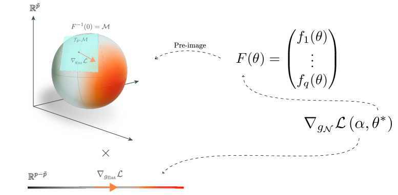
In this section, we explain how to incorporate constraints on a subset of the parameters directly into the ERM framework. In addition, we provide explicit examples of simple constraints, which may be used for instance to encode equivariance in Multi Perceptration Layers (MLPs).
Constraints
We consider constraints given in the form of a system of equations. More explicitly, let be a twice continuously differentiable map, where denotes the number of constrained parameters and is the number of equations. We assume that . For notational convenience, we decompose , where the first and second subspaces correspond to the unconstrained and constrained parameters, respectively. We take and to be the projections onto the unconstrained and constrained parameter subspace, respectively. We will denote the unconstrained and constrained parameters by and , respectively, i.e., and . The constrained ERM problem is defined below.
Definition 2.2 (CERM).
Let be a continuously differentiable parameterization of admissible mappings and a twice continuously differentiable constraint, where . Suppose is a continuously differentiable loss function. The constrained ERM problem for with respect to is defined by
| (2) |
Note the generality of the admissible mappings in Definition 2.2. Although we will focus on neural networks from now on, the proposed framework applies to any parametric model, e.g., logistic or polynomial regression models. Next, we show that the CERM problem in (2) can be reformulated as an ordinary ERM problem on a Riemannian manifold , provided that the system of equations satisfies a mild non-degeneracy condition. This result allows us to consider the admissible parameters as a geometric object in its own right, whose intrinsic geometry we exploit to solve (2).
Theorem 2.3.
If zero is a regular value of , then the CERM problem in (2) is equivalent to solving an ordinary ERM problem on a Riemannian manifold of dimension . Here is an embedded -submanifold of and . The equivalent minimization problem is given by
| (3) |
where is the inclusion map.
Proof.
The solution set is an embedded -submanifold of of dimension by the Implicit Function Theorem, since zero is a regular value of . A detailed review of this statement is provided in Theorem 2.6. Since is naturally embedded in , we may endow it with the pull-back metric , turning it into a Riemannian manifold . Here , where is the standard Euclidean metric on . The constrained ERM problem can now be reformulated as an ordinary ERM problem on the product manifold . Note that . Here is the product metric and corresponds***Formally, we should incorporate the dimension into the notation for the flat metric on . However, to avoid clutter in the notation, we will denote the standard Euclidean metric on any finite-dimensional vector space in the same way. to the standard Euclidean metric on . Altogether, having these geometric structures in place, the CERM problem in (2) is equivalent to (3), which proves the statement. ∎
For convenience, we shall from now on refer to the objective in (3) as simply the loss. We end this section with two simple examples of constraints that fit into our framework.
Example 2.4 (Equivariance).
For our first example, we show how to constrain layers in MLPs to be equivariant with respect to a given family of commuting operators . A well-known example is the case when consists of circular shifts on , which corresponds to translation equivariance. To illustrate the technique, we consider a fully connected (pre-activated) layer without bias, i.e., , for some weight matrix . In this setup, there are no unconstrained parameters and . We require that for all and . This is equivalent to for all .
To set up constraints, we assume there exists an operator which has simple eigenvalues. In this case, has linearly independent, possibly complex-valued, eigenvectors . For such an operator, it is straightforward to show that commutes with if and only if there exists a change of basis in which both operators are diagonal. More precisely, the commutator if and only if is diagonal, where are eigenvectors of . This implies in particular that is diagonal for all .
The latter observation provides a convenient method for imposing the desired constraint; we simply need to ensure that is diagonal. We consider the case that is complex-valued. The real-valued case is dealt with similarly. Define , where , by
Then if and only if is diagonal. Furthermore, if zero is a regular value of , then is a complex analytic manifold of dimension . This manifold can be identified with a real-analytic manifold of dimension , which directly fits into our framework. In particular, since we seek real-valued operators, we set equal to either the real or imaginary part of , which both commute with all operators in .
As a concrete instantiation of this method, we consider the case of translation equivariance again, where is the set of circular shifts on . We choose to be the left-shift operator, which has simple eigenvalues; the -th roots of unity. An associated collection of eigenvectors is given by
Of course, for translation equivariance, we can solve the equation by hand, and show that needs to be a so-called Toeplitz or circular matrix. This is equivalent to the statement that needs to be a convolutional layer.
Example 2.5 (Orthogonal filters).
In the next example, we consider the work of [25], where filters of a CNN were initialized to be orthogonal. While not the intention of their paper, we can use the CERM framework to extend the orthogonality beyond initialization. The constraints are relatively easy to set up, complementing the more involved constraints considered in our main application. This example may be interpreted as a warm-up towards our MRA example in Section 3.
Consider a convolutional layer with filters of size , where . We require that the filters are orthonormal throughout the entire training process. To be more precise, consider the case of one filter . We require that This is equivalent to the following system of equations:
for each . Motivated by this observation, we define by
and by . Then zeros of correspond to orthonormal filters. In this example, there are no unconstrained parameters, i.e., . Furthermore, and . The pre-image is a smooth manifold of dimension , referred to as the orthogonal group .
2.3 Relation to Lagrange Multipliers
We briefly compare our strategy with a related alternative, namely the method of Lagrange Multipliers. Lagrange Multipliers can be understood from a geometric perspective by essentially writing down the necessary conditions for stationarity in a special local chart, namely one in which is embedded into as the graph of the inverse chart. The resulting necessary conditions for a point to solve (2) is the existence of a so-called Lagrange multiplier so that
| (4) |
Here we have defined by .
The system of equations in (4) is referred to as the Karush–Kuhn–Tucker (KKT) conditions. For general nonlinear problems, the KKT-conditions constitute a highly nonlinear system of equations and are difficult to solve directly. Many techniques for solving the constrained problem in (2) are based on adaptations of Newton’s method for (4), e.g., Sequential Quadratic Programming (SQP) or Interior Point methods to name a few, see [26] for more. The dynamics of such algorithms, i.e., the behavior of the generated sequence of points, takes place in a higher dimensional space than what we started with and is largely determined by Newton’s method for solving (4).
Our approach is fundamentally different from such methods in the following sense. Firstly, the dynamics of our optimization scheme takes place on a lower dimensional submanifold defined by the constraints. Once we have initialized any initial point on , we use the intrinsic geometry of the manifold to find a next point by following descent trajectories confined to the manifold, e.g., geodesics. We therefore satisfy the desired constraints throughout the entire optimization procedure thereby exploring the space of feasible parameters directly. Finally, the dynamics of our algorithm is completely determined by the (negative) gradient flow of the objective, and not by Newton’s method for (4).
2.4 Graph coordinates on
In this section we explain how to construct a special (local) coordinate system, a so-called graph chart, on around a point . This chart will be used extensively to perform numerical computations, e.g., to evaluate the Riemannian metric . The existence of this special chart is guaranteed by the Implicit Function Theorem and naturally comes up in the proof of the so-called Pre-Image Theorem [27], which provides sufficient conditions for to be an embedded submanifold of . Below, we will essentially repeat the proof of this theorem, in a somewhat simplified setting, see [27] for the slightly more general case dealing with smooth maps between general manifolds. The reason for including an explicit proof is that the computational steps form the backbone of our method.
Theorem 2.6 (Pre-image theorem).
Let be a map of class , where . If zero is a regular value of , then is an embedded -submanifold of of dimension .
Proof.
Assume zero is a regular value of and let be arbitrary. Then must have linearly independent columns. For the sake of concreteness, assume
| (5) |
is an isomorphism on , where and . This gives rise to the decomposition , where the first subspace corresponds to the coordinates with multi-index , and the second subspace contains the remaining coordinates. Let and denote the projections onto the first, and second subspace, respectively, and write and for the corresponding coordinates. We may then view as a function of . More formally, we define a new map by , where is a permutation which puts the coordinates back in the original ordering.
Next, write , and observe that is an isomorphism on by construction. Therefore, by the Implicit Function Theorem, there exists a unique -map , where is an open neighborhood of , such that and for all . Altogether, this shows that the map defined by is a local parameterization of , i.e., its inverse is a local chart on . Therefore, since is arbitrary, it follows from this observation that is an embedded -submanifold of dimension . ∎
Remark 2.7 (Relaxation).
Strictly speaking, one still needs to show that is open in , and that there is a chart in the ambient manifold in which is locally described by setting the first coordinates to zero. We omitted the details because they follow in a straightforward manner from our arguments. In particular, the proof of Theorem 2.6 also shows that we may relax the condition that zero is a regular value of . Specifically, let be the set of regular points of . If , then is an embedded -submanifold of of dimension .
Remark 2.8 (Graph coordinates and Lagrange Multipliers).
The coordinates associated with the chart are commonly referred to as graph coordinates since is locally parameterized by the graph of . The existence of Lagrange Multipliers can be proven by writing the necessary conditions for stationarity of the objective in (2) in this chart.
Remark 2.9 (Regularity).
If is or analytic, then the manifold inherits the same regularity.
Throughout this section, we assume that zero is a regular value of , which guarantees that is (an embedded) Riemannian manifold. In the discussion below, we will consider a point , and explain how to explicitly evaluate the Riemannian metric at this point relative to the chart . In turn, this will enable us to compute gradients. To avoid clutter in the notation, we henceforth assume without loss of generality, that the first components of are linearly independent, i.e., , and hence . Note that this assumption will hold on an entire open neighborhood of . For points outside this neighborhood, one needs to choose another set of components that constitute a linearly independent system, thereby obtaining a different chart .
In practice, we do not have an explicit formula for the chart constructed in Theorem 2.6. Nonetheless, we can compute with it implicitly as explained below. For the sake of illustration, however, we will first consider a toy example before we proceed, in which explicit computations and formulae are available. We will continue this example throughout this section to complement the otherwise abstract numerical recipes.
Example 2.10 (The unit sphere ).
Consider the map defined by . Clearly, corresponds to the unit sphere . We will use Theorem 2.6 to prove that is a two-dimensional embedded submanifold of . While one can easily prove this by constructing explicit charts, e.g., using stereographic projection or polar coordinates, our goal is to demonstrate how to use Theorem 2.6 and explicitly construct the chart .
First observe that . Further note that for any at least one of the components must be nonzero. Therefore, is surjective for all , i.e., zero is a regular value of . Consequently, is a -dimensional embedded submanifold of by Theorem 2.6. Moreover, without explicitly constructing charts, we immediately see that is a -manifold (analytic even), since is a -map. The chart from the proof is easily constructed in this case. To see this, suppose , then , and . The (maximal) domain of this chart is .
2.5 Riemannian metric on
In this section we express the product metric on in local coordinates with respect to the chart . Here denotes the identity map on . We start by deriving a representation of relative to . For this purpose, denote the coordinates associated to by , and the standard coordinates on by . Recall that the pullback metric on is given by . Therefore, in local coordinates, we have where is given by
where we recall that is a local parameterization of the manifold. In practice, we are only interested in a specific choice for , namely . For this choice, the chart is explicitly known: . Hence, to evaluate the metric at , we need to explicitly compute .
To evaluate , first observe that for any . Here denotes the identity matrix. Furthermore, we can compute the derivative of by using its defining property (see the proof of Theorem 2.6)
More precisely, differentiating both sides of this equation and evaluating at yields
| (6) |
Both and can be explicitly evaluated. Moreover, is a non-singular matrix. Hence we can compute by solving the linear system of equations in (6). Subsequently, we can explicitly evaluate the components of the Riemannian metric at :
| (7) |
Finally, we evaluate the product metric on relative to at :
| (8) |
where is the symmetric matrix whose component is given by .
Example 2.11 (The unit sphere - continued).
We end this section by continuing Example 2.10 and computing the components of the Riemannian metric relative to . This computation is only included to provide a concrete application of the abstract theory above. In practice, the computations, e.g., solving the equation in (6), are implemented numerically. Now, a straightforward computation shows that
Therefore, the components of the Riemannian-metric relative to are given by
2.6 Computing gradients on
In this section we explain how to compute the gradient of a smooth map relative to . For notational convenience, we denote the coordinates associated to by , where and are the coordinates associated to and , respectively. In the next section, we will use these computations to find a minimizer of using SGD. We remind the reader that our specific use case is the constrained ERM problem in (2), which corresponds to finding a minimum of
The gradient of on with respect to is the unique vector field satisfying . Such a vector field must exist since is non-degenerate. In local coordinates,
where are smooth (uniquely determined) functions. We can easily determine these functions by plugging them into the defining equation for the gradient and evaluating both sides at . This yields the following linear system of equations:
Here are the components of relative to . Similar as before, we define to be the symmetric matrix whose component is given by . Then
where are the components of the inverse of .
In practice, of course, we will not invert the matrix . Instead, we numerically solve the system of equations at our point of interest for the unknown-coefficients by exploiting the block structure of the metric, see (8). In particular, we immediately see that the first components of are given by , where . In other words, since the metric on is flat, the associated components of the gradient reduce to the usual ones. On the other hand, for the coordinates on , we have
by (8). Therefore, the last components of can be obtained by solving the linear (square) system
| (9) |
Computing partial derivatives
We need one final ingredient to compute the gradient of . Namely, we need to evaluate its partial derivatives with respect to the coordinate system defined by . Clearly there is no difficulty in computing , since are the standard coordinates on , and thus correspond to the “usual” partial derivatives one encounters in calculus on vector spaces. For the partial derivatives with respect to , however, we have to be more careful, and compute from the perspective of the (non-trivial) chart:
| (10) |
since and . In the last line we assumed that has a smooth extension to some open neighborhood of for all . This is the case for all our applications, where comes from the constrained minimization problem in (2).
Altogether, we now have all the ingredients to numerically evaluate the gradient of a smooth map relative to the chart . The steps are summarized in Algorithm 1.
Example 2.12 (The unit sphere - continued).
We continue our example of the unit sphere and explain how to compute the gradient of a smooth map . We assume that can be smoothly extended to an open neighborhood of in . To compute the gradient relative to , we need to solve the system in (9). For this purpose, we first explicitly compute the inverse of :
Again, we stress that in practice, we do not invert this matrix, but solve the system of equations numerically instead. Next, we compute the partial derivatives of relative to using (2.6):
Here denote the partial derivatives with respect to the standard coordinates on , i.e., these are the “usual” partial derivatives from calculus on vector spaces. Hence
where
2.7 Stochastic Gradient Descent
In this section we explain how to perform SGD on Riemannian manifolds using graph coordinates. For previous work on SGD on Riemannian manifolds, we refer the reader to [18, 19, 20, 21, 22]. The presented technique is completely intrinsic to the manifold and involves following (approximate) geodesics in the direction of the (negative) gradient of . To explain this idea in more detail, we first briefly recall the notion of geodesics and refer the reader to [28, 27] for a more comprehensive introduction to differential geometry.
2.7.1 Geodesics and parallel transport
The analog of a gradient descent step on a Riemannian manifold is to follow “a straight line”, confined to the manifold, in the direction of the negative gradient. In order to make sense of this, one first needs to generalize the notion of a straight line to arbitrary Riemannian manifolds. On Euclidean vector spaces, one can define a straight line as a curve whose velocity is constant. This notion makes sense on a vector space, since different tangent spaces can be related to one another, but does not make sense on a general manifold. An equivalent notion, which can be generalized to a Riemannian manifold, is to define a straight line as a curve whose acceleration is zero. The key idea here is that the notion of acceleration can be made sense of on any Riemannian manifold. More precisely, one can define a so-called affine connection or covariant derivative , not to be confused with the notation for a gradient, which allows one to measure the change of one vector field in the direction of another. Formally, a connection is a differential operator , which is -linear in the first variable, -linear in the second, and satisfies the Leibniz rule. Given two vector fields , one typically writes and interprets this new vector field as measuring the change of in the direction of .
A connection is a so-called local operator in the sense that is completely determined by and the behavior of in a neighborhood around . We may therefore write . This local property can in turn be used to measure the change of a vector field in the direction of a curve. More precisely, given a curve , there exists a unique (differential) operator associated to and , which enables one to differentiate vector fields in the direction of . This operator is uniquely determined by three properties: it is -linear, satisfies the Leibniz rule, and if can be extended to a vector field defined on an open neighborhood of , then . One can now make sense of acceleration by defining it as the derivative of the velocity field in the direction of itself, i.e., acceleration is defined by . A “straight line” or geodesic is then simply defined as a curve whose acceleration field is zero. The existence of geodesics is guaranteed, at least locally, by the existence and uniqueness theorem for ODEs, see the discussion below.
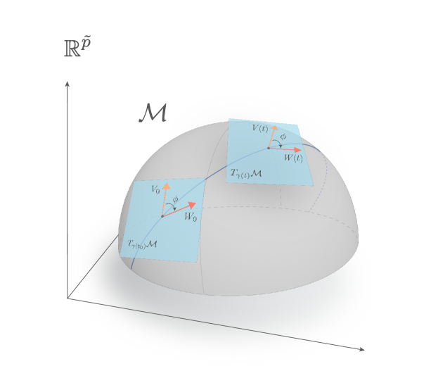
A covariant derivative allows one to generalize many more familiar concepts from Euclidean vector spaces to Riemannian manifolds. For instance, given a curve and tangent vector , one may extend to a vector field which “is parallel” to everywhere, see Figure 2. This extension is referred to as the parallel transport of along . The notions of geodesics and parallel transport, however, heavily depend on the choice of connection. In general, there exist infinitely many connections on a Riemannian manifold. There exists exactly one connection, however, the so-called Levi-Civita connection, which in a sense is “naturally aligned” with the Riemannian metric. This specific connection may be summarized in a geometric way by the following two conditions, which are usually taken for granted on Euclidean spaces. First, if is a curve and are tangent vectors with angle between them, then the parallel extensions must have angle between them as well at any point on (metric compatibility), see Figure 2. Secondly, for any coordinate chart on , the rate of change of one coordinate direction in the direction of another must not change if we swap directions (torsion free). In this paper we always use the Levi-Civita connection.
Finally, we provide a local description of a geodesic . Let and assume is any chart containing , then there exists a such that . Write and observe that for each , there exist smooth functions such that , since is a frame on . The coefficients are called the Christoffel symbols of on . They completely characterize the connection on . The equation for a geodesic starting at an initial point with initial velocity is given by
| (11) |
see [28]. Here we have expressed and the components of its velocity in local coordinates:
This is a second-order ordinary differential equation for the unknown curve (geodesic) . In general, this equation is nonlinear. The existence and uniqueness theorem for ODEs only guarantees the existence of a local solution. The solution may be extended outside of by considering other charts. However, due to the nonlinearity, there may be obstructions to extending the solution beyond a certain point. In general, there is no guarantee that a geodesic can be extended and defined for all . A manifold with the property that geodesics exist for all time is called complete. In particular, any compact manifold is complete [28]. We remark that for the purpose of SGD local existence is sufficient, since we need to take sufficiently small steps on the manifold to guarantee descent of the objective.
2.7.2 Gradient descent steps
We will now explain how to define a gradient descent step on our manifold of interest by computing approximate solutions of the geodesic equation (11). The main idea is to follow the geodesic starting at our current point in the direction of the negative gradient , for a small amount of time. While there exist many efficient techniques to compute high order approximate solutions of ODEs, e.g., Runge-Kutta solvers, they typically rely on evaluating the associated vector field on a neighborhood of the initial condition. In our set up, this would correspond to evaluating the Christoffel symbols at different points on the manifold. While it would be possible to explore nearby points in our chart , e.g, by computing a second or higher order Taylor-expansion of , our objective is not to just simply explore . Instead, we are only interested in following paths on which lead to a decrease in . In particular, we are limited to choosing sufficiently small step-sizes, since we wish to stay on descent directions for . For this reason, since we only need to integrate the geodesic equation for small amounts of time, we use a first or second order Taylor-expansion to approximate the solution of (11).
More precisely, let denote the curve in local coordinates, then
as . For our particular case, we set
where are the components of the gradient relative to . We define the second order gradient descent step with step-size based at for by
Here is the coordinate representation of . Similarly, we define the first order gradient descent step with step-size based at by
Note very carefully that the gradient descent steps are taken in the local coordinate system. For sufficiently small , we are guaranteed that the new point is contained in the current chart for both the first and second order steps. However, to get back to the manifold, we have to evaluate . In addition, we also have to explicitly evaluate the Christoffel symbols. The computational details are given below.
2.7.3 Evaluating the inverse chart
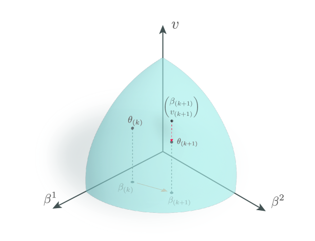
We will use a Taylor expansion to evaluate the inverse chart on at . Subsequently, we use Newton’s method to refine the approximation. The resulting point that we find must necessarily correspond to , and is thus completely determined by , since is locally unique as explained in Theorem 2.6. This justifies the claim made in Section 2.3 that the search dynamics of our algorithm is completely determined by the negative gradient flow of , since is.
Below we provide the computational details for the case of a second order Taylor expansion; the first order case is obtained by ignoring the second order terms. To avoid clutter in the notation, we will henceforth (interchangeably) write
This notation also emphasizes that we move from a given point at step to a next point.
The second order Taylor expansion of around is given by
as . We have explained in Section 2.5 how to explicitly compute , which was needed to evaluate the Riemannian metric. Here we employ the same strategy to compute the second derivative , where denotes the space of -valued -tensors on . We start by rewriting (6) as
Next, we differentiate both sides with respect to and evaluate at . This yields
| (12) |
for all . To compute the component of with respect to the standard basis, i.e., in order to compute , we evaluate both sides of (12) at and solve the equation
| (13) |
for each . This equation admits a unique solution, since is an isomorphism on .
Finally, we approximate using its second (or first) order Taylor expansion and then use Newton’s method to evaluate
More precisely, we first approximate by
| (14) |
We then refine this approximation by finding a zero of the map using Newton’s method and as initial guess. In particular, we solve the equation for , while remains fixed. The zero that we find must necessarily correspond to , since is locally unique as explained in Theorem 2.6. Altogether, this yields the desired point . See Figure 3 for a visualization of the steps described in this section.
2.7.4 Evaluating the Christoffel symbols
We end this section by explaining how to explicitly evaluate the Christoffel symbols at . Recall that a connection is locally completely characterized by the Christoffel symbols. The constraints that uniquely determine the Levi-Civita connection, i.e., metric compatibility and torsion-freeness, therefore also impose constraints on the Christoffel symbols. In fact, the standard proof for the existence of the Levi-Civita connection is constructive and establishes an explicit relationship between the Christoffel symbols and the Riemannian metric:
see [28, 27] for instance. We will use this expression to numerically evaluate the Christoffel symbols.
It follows immediately from the block structure of the metric in (8) that
for all . The reason why these coefficients are zero is because there is no interplay between the submanifolds and , which together make up , and because the metric on is flat. In particular, this shows that the component in of a geodesic on is just a straight line as expected.
It remains to consider the case , which is associated to the non-trivial metric on . We use the expression in (7) to compute the partial derivatives of the relevant components of . More precisely, observe that
for . We can evaluate this expression numerically, since we can explicitly evaluate and . Finally, to compute the relevant Christoffel symbols, we define vectors for each by
The remaining (non-zero) Christoffel symbols associated to can now be computed by solving the following linear system of equations:
3 Multiresolution Analysis and CERM
In this section we present a non-trivial application of the CERM framework to learn optimal wavelet bases for a given task. Specifically, we explain how to set up a system of equations (constraints) whose solution set corresponds to wavelets. To set up appropriate constraints, we first review the needed theory from Multiresolution Analysis (MRA) [29, 30, 31]. Multiresolution analysis provides a natural framework for defining and analyzing wavelets. Moreover, it can be used to characterize a large class of finitely supported wavelets as solutions of a finite system of equations. We review in detail how to derive these equations and how to efficiently compute wavelet decompositions using Mallat’s Pyramid Algorithm [29], which together form the backbone of our main example in Section 4, where we train networks for predicting wavelet decompositions of contours in the medical domain. Before we continue, however, we briefly discuss examples of tasks where wavelets arise naturally.
Applications of MRAs
There are several tasks at which one expects wavelet-based neural networks to excel. Wavelet decompositions naturally lend themselves to representing continuous objects such as curves, images, vector fields, or other higher-dimensional objects. Hence any task where the object of interest can be identified with a smooth or continuous function is well-suited for wavelet-based neural networks. There is an abundance of such examples to be found in computer vision, e.g., boundary prediction, image registration, and so forth. Another family of interesting applications can be found in signal analysis, e.g., in compression and denoising, where wavelets are long-standing tools that have proven to be extremely efficient [29]. The main idea in these areas is to extract information about noise, smoothness, and even singularities, through analysis of the wavelet coefficients. Subsequently, by modifying a subset of the coefficients, e.g., through thresholding, the signal can be “cleaned up” or denoised.
In this paper, we consider one-dimensional wavelets only, which will be applied to boundary prediction of simply-connected two-dimensional domains in Section 4. The wavelet framework, however, is easily adapted to higher-dimensional domains, such as images, by using tensor products of the one-dimensional bases.
3.1 Multiresolution Analysis
In this section we briefly review what Multiresolution Analyses (MRA) are, how wavelets come into play, and why they are useful. We closely follow the exposition in [31, 30] and refer the reader to these references for a more comprehensive introduction.
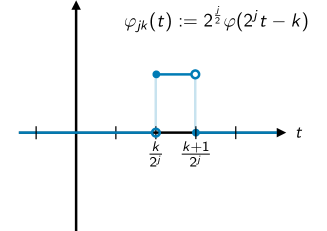
The uncertainty principle in Fourier analysis states that a signal cannot be simultaneously localized in the time and frequency domain. Multiresolution analysis aims to address this shortcoming by decomposing a signal on different discrete resolution levels. The idea is to construct subspaces , associated to various resolution levels , spanned by integer shifts of a localized mapping . The level of localization associated to is determined by taking an appropriate dilation of a prescribed map ; the so-called scaling function. In the MRA framework the dilation factors are chosen to be powers of two. Formally, we require that is an orthonormal basis for , where , see Figures LABEL:fig:scaling_function and LABEL:fig:approx_subspace. Altogether, this yields an increasing sequence of closed subspaces dense in , where is the next level up in resolution after . For the sake of completeness, we provide the formal definition of a MRA below.
Definition 3.1 (Formal definition MRA [29]).
Let and denote the translation and normalized dilation operator, respectively, defined by and for and . A multiresolution analysis of is an increasing sequence of subspaces , such that
-
(i)
,
-
(ii)
is dense in ,
-
(iii)
if and only if ,
-
(iv)
is invariant under translations,
-
(v)
such that is an orthonormal basis for .
Condition formalizes the idea that any signal in can be arbitrarily well approximated using an appropriate resolution level. Condition encapsulates the idea that is the next resolution level with respect to our choice of dilation operators , i.e., there are no other resolution levels between and . Combined with it implies that each subspace is invariant under integer shifts. Finally, condition formalizes the idea that the subspaces are spanned by translations and dilations of the map ; the so-called scaling function or father wavelet. Indeed, it is straightforward to show that is an orthonormal basis for , where .
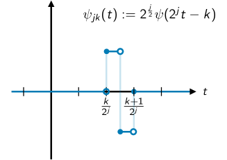
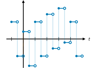
Decomposing a signal
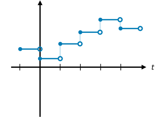
Next, we explain how the MRA framework can be used to analyze a signal . The main idea is to approximate at different resolution levels by projecting it onto the subspaces . More precisely, we define the approximation of at resolution level by , where is the orthogonal projection onto (see Figure LABEL:fig:approx_subspace). The coefficients of with respect to the basis for , denoted by , are called the approximation coefficients of at level .
To study the information that is lost when a signal in is projected onto , we consider the operator . The range of is denoted by and referred to as the the detail subspace at level (see Figure LABEL:fig:_detail_subspace). The subspace is the orthogonal complement of in . The detail subspaces are mutually disjoint and orthogonal by construction. Furthermore, since for any , it follows that
| (15) |
This decomposition shows that a signal on resolution level can be reconstructed from any lower level if all the details in between are known.
A fundamental result, known as Mallat’s Theorem, states that the subspaces can also be spanned by dilating and shifting a single map. More precisely, there exists a map , the so-called mother wavelet, such that is an orthonormal basis for , see [30]. Here we have used the notation as before. The coefficients of with respect to the basis for , denoted by , are referred to as the detail coefficients of at resolution level . The detail coefficients store the information needed to go back one level up in resolution.
Remark 3.2.
We will frequently omit the dependence of the approximation and detail coefficients on the underlying signal , i.e., write and , whenever there is no chance of confusion.
In general, given approximation coefficients at level and detail coefficients at levels , we can reconstruct the approximation at level using (15):
Altogether, these observations give rise to the following terminology:
Definition 3.3 (Multiresolution decomposition of a signal).
Let be resolution levels. A finite -multiresolution decomposition of a signal is the sequence
3.2 The scaling equation
In this section we review the so-called scaling equation, which is key for understanding many fundamental aspects of MRAs, both theoretical and computational. We will heavily rely on it in the subsequent sections to set up the desired constraints and to efficiently compute with wavelets. The key observation is that since , there exists a unique sequence such that
| (16) |
This equation is referred to as the scaling equation; one of the fundamental properties of a scaling function.
Low and high pass filters
The sequence is called the low-pass filter of the MRA. It completely characterizes the scaling function and therefore also the corresponding MRA. We will often refer to as simply a wavelet filter. Similarly, since , there exists a unique sequence , the so-called high-pass filter associated to , such that
| (17) |
For Mallat’s mother wavelet, we have . In practice, to define a MRA, one only needs to specify an “appropriate” low-pass filter . In Section 3.4 we derive a finite set of equations whose solutions correspond to low-pass filters, provided a mild non-degeneracy condition is satisfied, and characterize a finite-dimensional family of compactly supported wavelets.
Example 3.4 (Haar MRA).
A simple example of a MRA is the so-called Haar MRA; the father wavelet is given by , and the mother wavelet by . They are visualized in Figure LABEL:fig:scaling_function and Figure LABEL:fig:mother_wavelet, respectively. The associated low and high pass filters are given by
respectively.
The refinement mask
An important observation follows from taking the Fourier Transform of the scaling equation, which yields
| (18) |
Here is a 1-period map typically referred to as the refinement mask. Throughout this paper, we shall abuse terminology and frequently refer to both and as the low-pass filter associated to . Both the low-pass filter and refinement mask completely characterize the scaling function. The relation in (18) will be used extensively in Section 3.4 to derive constraints on admissible filters.
Existence and uniqueness of MRAs
The scaling equation plays a seminal role in establishing the existence and uniqueness of an MRA given a candidate for a low-pass filter. While there is no need to explicitly construct , we do briefly discuss its existence here to justify the claim that we are learning wavelets. In addition, the discussion will reveal a necessary condition on . The idea for proving the existence of a scaling map , given a low-pass filter , is to “reconstruct” its Fourier transform using the scaling equation. To see how, suppose we start with a scaling map . Then repeated application of (18) yields
Assuming that is continuous at , we may consider the limit as , which yields
| (19) |
provided the latter product exists. Since is not identically zero, we must have that . This imposes a constraint on , namely . Without loss of generality, we may further assume that .
Conversely, if we start with a sequence instead of a scaling map , we may try to use the right-hand side of (19) to define a candidate for . More precisely, if the infinite product converges to a map in , one may use the inverse Fourier transform to define a corresponding candidate for . As it turns out, if decays sufficiently fast to zero, and we assume that , where we now define via (18), then is in , continuous at , and satisfies (19). For a more precise statement, we refer the reader to [32, 31]. In this paper, we exclusively deal with finite sequences , for which these assumptions are always (trivially) satisfied. Hence we may use (19) to define a candidate for a scaling map . However, we still need to impose additional constraints on , to ensure that the translates of are orthogonal, see Section 3.4.
3.3 The Discrete Wavelet Transform


The scaling equation (16) can be used to derive an efficient scheme for computing a (finite) multiresolution decomposition of a signal . More precisely, given initial approximation coefficients at level , the scaling equation can be used to compute the approximation and detail coefficients at level . Conversely, the orthogonal decomposition can be used to reconstruct given the approximation and detail coefficients and , respectively, at resolution level . The mapping associated to these operations is called the (-level) Discrete Wavelet Transform (DWT). It provides an efficient way to obtain a multiresolution decomposition of a signal. The associated algorithm, which iteratively applies the -level DWT, is known as the so-called Pyramid Algorithm [29].
Decomposition
Let be approximation coefficients at an initial resolution level , where . To obtain the approximation and detail coefficients at level , we first note that
| (20) |
This relation between and can be easily derived by substituting the right hand side of the scaling equation (16) into the definition of . Consequently,
| (21) |
where denotes the two-sided discrete convolution and is defined by . The resulting map is typically referred to as the DWT at level . An analogous computation for the detail coefficients shows that
| (22) |
The decomposition of the approximation coefficients at level into approximation and detail coefficients at level is illustrated in Figure LABEL:fig:pyramid_down.
Reconstruction
The inverse DWT can be derived in a similar fashion using the decomposition . To make the computation explicit, we use (17) and the scaling equation again to write
Consequently, since ,
where is defined by
This shows that the approximations coefficients at level are given by
The reconstruction procedure is schematically shown in Figure LABEL:fig:pyramid_up.
Remark 3.5 (Numerical implementation DWT).
The convolutions appearing in the decomposition and reconstruction formulae can be efficiently computed using the Fast Fourier Transform (FFT), see Appendix A.
3.4 Setting up constraints for wavelet filters
In this section we set up a finite system of equations whose zeros, under a mild non-degeneracy condition, correspond to wavelet filters. Recall that a wavelet filter is a sequence that characterizes a scaling function . We reformulate the key requirements on , namely that its translates are orthogonal and , in terms of its low-pass filter . In turn, this imposes constraints on admissible filters in the form of a system of equations. Solutions of this system are commonly referred to as Quadratic Mirror Filters (QMFs), see Definition 3.8. We remark that these equations and conditions are well-known and refer the reader to [31, 30] for a more comprehensive treatment.
To reformulate the orthogonality conditions into a system of equations for , we first rewrite the system in frequency space. The recurrence relation for the Fourier transform of in (18) may then be used to derive a necessary condition on the refinement mask . Subsequently, we can reformulate this necessary condition as an equivalent condition on . The details can be found in [30]. Here we only state the relevant results.
Lemma 3.6 (Orthogonality refinement mask).
Suppose satisfies the dilation equation for a refinement mask with Fourier coefficients . If the family is orthonormal, then
| (23) |
for a.e. .
Proof.
See [30]. ∎
Remark 3.7.
The condition in (23) is often referred to as the Quadratic Mirror Filter condition.
Definition 3.8 (Quadratic Mirror Filter).
A Quadratic Mirror Filter (QMF) is a sequence which satisfies (23) and .
The reason for introducing this terminology is that QMFs correspond to wavelet filters under an additional non-degeneracy condition. Here we only state the result for finite filters.
Theorem 3.9.
Suppose is a finite QMF. If , then
is a scaling function and defines an MRA of . Here denotes the Fourier transform.
Proof.
See [33] Theorem . ∎
Remark 3.10.
One may expect that any finite filter satisfying (23) will define a scaling function whose translates are orthogonal. However, this is unfortunately not the case, and the additional requirement that is needed to avoid degenerate cases.
Next, we derive a system of equations for that is equivalent to (23). To formulate this system of equations, we define operators by and . For brevity, we will frequently write as before. Even though we are dealing with real-valued filters in practice, below we state the results for general complex-valued sequences.
Lemma 3.11 (Orthogonality low-pass filter).
Suppose is a refinement mask with Fourier coefficients . Then the orthonormality constraint in (23) is equivalent to the following system of equations:
| (24) |
Proof.
We start by computing the Fourier coefficients of the lefthand-side of (23). To this end, observe that the 2-periodic map and its conjugate have Fourier coefficients and , respectively. Therefore, since , the product is with Fourier coefficients . Similarly, the Fourier coefficients of are given by . Hence
Unfolding the definitions yields
Note that whenever is odd, since
| (25) |
The equation in (23) is equivalent to the statement that for , since the Fourier coefficients of a -function are unique. Hence (23) is equivalent to for by the observation in (25). Finally, the latter statement is equivalent to for , since
for any . The two cases in (24) show the demands for and positive even indices, respectively. This establishes the result. ∎
Remark 3.12.
QMF conditions
We are now ready to set up the desired constraints. In general, the QMF conditions are not sufficient to guarantee that is the low pass filter of a scaling function, see the discussion in Remark 3.10. However, in numerical experiments, we never seem to violate the non-degeneracy condition when only imposing the QMF conditions. For this reason, the only constraints that we impose are the QMF conditions. We do provide an option to include the non-degeneracy condition in Remark 3.15.
To properly write down the QMF conditions as constraints on a sequence , we introduce some additional notation. Let denote the space of one-dimensional -valued two-sided sequences of order , i.e.,
Note that is a vector space over of dimension . In particular, . The reason for introducing this notation is to explicitly keep track of the two-sided ordering of sequences. We are now ready to gather all the demands that we have derived, and place them into the general framework of Section 2.
Definition 3.13.
Let be a prescribed order. The QMF-map is the function defined by
The first equations correspond to the orthonormality constraints. Note that we only have to impose for , since for . The last equation corresponds to the condition that . The set of regular points in is a real-analytic -dimensional submanifold of by Remark 2.7. In particular, we can get as many degrees of freedom as desired by choosing a sufficiently large order .
We summarize the interpretation and importance of the constraints in a theorem.
Theorem 3.14.
If and , then is the low-pass filter of a scaling map .
Remark 3.15 (Imposing the non-degeneracy condition).
The additional non-degeneracy condition can be imposed, for instance, by requiring that has no zeros in . Since we consider finite filters only, the refinement mask is analytic (entire even). Hence the latter condition may be imposed by requiring that
| (26) |
where is an ellipse with foci and and is a free parameter which controls the sum of the major and minor axis. We remind the reader that the above integral counts the zeros of (up to a scaling factor) in , provided has no zeros on . For any parameterization of , we can numerically evaluate the integrand of (26) on an associated uniform grid by using the Fourier expansion of . We may therefore numerically compute a Fourier expansion of the integrand, which in turn allows numerical approximation of the contour integral.
4 Contour Prediction using MRA
In this section we present a non-trivial application of the CERM framework to learn optimal wavelet bases for contour prediction in medical images. Wavelets have, as discussed in the previous section, the ability to represent signals at multiple resolution levels, allowing for both detailed analysis of local features and a broad overview of the overall signal. This ability makes wavelets an ideal tool for contour prediction in two-dimensional images, such as slices of CT or MRI scans.
In the context of contour prediction, wavelets can be used to represent the boundary of a region in an image using a simple closed curve. While a Fourier basis appears to be a natural candidate for this task, its global nature impedes accurate predictions of curves that exhibit highly localized behavior, requiring accurate estimates of small noisy high-frequency modes. For this reason, we have chosen to represent contours using MRA and wavelets. More precisely, we consider two-dimensional gray-valued images , e.g., slices of MRI or CT scans of size . We assume that each image contains a (uniquely identifiable) simply connected region , e.g., an organ, with boundary . It is assumed that can be parameterized by a simple closed piecewise -curve . We will develop a deep learning framework for computing such parameterizations by learning a multiresolution decomposition of using the methods developed in Sections 2 and 3.
This section is organized as follows. In Section 4.1 we explain how to represent periodic curves using wavelets. In Section 4.2 we provide details about the data, e.g., how ground truth curves are constructed, what preprocessing steps are taken, etc.. In Section 4.3 and Section 4.4, we present the full details of our network architecture and training schedule. Finally, in Section 4.5, we examine the performance of our auto-contouring models for the spleen and prostate central gland. In addition, we visualize the task-optimized wavelets.
4.1 Wavelet Representations of periodic curves
We start by explaining how to compute a multiresolution decomposition of a scalar-valued periodic signal with period . First, we address the issue that periodic signals are not contained in by considering the cut-off , which is contained in . In general, such a cut-off will introduce discontinuities at the boundary points and . These artifacts do not present an issue for us, however, since (by periodicity) we can restrict our analysis to a strict subset of length .
To compute a multiresolution decomposition of using the DWT, we need to compute the approximation coefficients of at some initial resolution level . To explain how such an initial approximation can be obtained in the first place, we derive an explicit formula for the approximation coefficients . While we will not directly use this formula, we do remark it can be efficiently implemented and provides an alternative method to initialize wavelet coefficients thereby addressing the so-called wavelet crime [34, 35]. For our purposes, this expression will be key for identifying which coefficients to consider, i.e., which spatial locations associated to are relevant for representing .
Lemma 4.1 (Initialization approximation coefficients).
Let be the scaling map of an MRA with low-pass filter and associated refinement mask . Assume is nonzero for only a finite number of indices so that for some . If is a -periodic map with Fourier coefficients , then
| (27) |
for any and , where is the angular frequency of .
Proof.
Let and be arbitrary. A change of variables shows that
since . Note that the latter holds for all . For in particular, we have that for all . Therefore, for such , we may plug in the Fourier expansion for and compute
Next, note that that series inside the integral converges pointwise to on . Furthermore, the partial sums can be bounded from above on by a constant, since and is bounded. Therefore, we may interchange the order of summation and integration by the Dominated Convergence Theorem:
Finally, changing the domain of integration to again, we see that
The stated result now follows from the observation that holds pointwise for any , since is nonzero for only a finite number of indices, see [31] Theorem . ∎
Remark 4.2.
It is straightforward to show that the partial sums converge uniformly on . It is therefore not needed to resort to the Dominated Convergence Theorem.
Remark 4.3.
The bounds and are the smallest and largest integer, respectively, for which the Fourier series for can be plugged into . The bounds are somewhat artificial, however, since the argument may be repeated for any cut-off of on , where . The choice for is ultimately irrelevant, however, since we are interested in the minimal number of approximation coefficients needed to cover ; see the discussion below.

Lemma 4.1 provides a convenient way to initialize approximation coefficients. To explain how, we first re-parameterize to have period and consider the cut-off . The motivation for this re-parameterization is that we can now conveniently relate specific approximation coefficients to sample values of . To be more precise, recall that is continuous at zero and . Therefore, if the initial resolution level is sufficiently large, the infinite product in (27) will be close to (for small ). Furthermore, in practice, we have a finite number of Fourier coefficients, i.e., for . Therefore, if is sufficiently large relative to , then
| (28) |
That is, on sufficiently high-resolution levels the approximation coefficients are close to the (scaled) sample values of the underlying signal; a well-known general fact of MRAs. Consequently, the approximation coefficients needed to cover (approximately) are . Motivated by this observation, and the fact that we only need on , we use the scaled sample values in (28) to initialize the coefficients , which cover approximately, see Figure 6.
We stress that in order for the above approximations to be accurate, the initial resolution level needs to be sufficiently large. Furthermore, to ensure that and , we require that
One can explicitly express the support of in terms of the order of the wavelet. Specifically, the scaling relation can be used to shown that , thus providing explicit values for and . A rigorous proof is out of the scope of this paper and we refer the reader to [33] Theorem .
Finally, we remark that after the initial approximation coefficients are initialized, the periodicity of has to be taken into account in the implementation of the DWT, see Appendix A.1 for the details.
4.2 Data and preprocessing
We have used public datasets from the Medical Decathlon Challenge [36] to illustrate the effectiveness of the CERM methodology. The selected data consists of CT scans of the spleen of size and T2-weighted MRI images of the prostate central gland, henceforth abbreviated as just the prostate, of size . The scans were cropped to size and , respectively. Furthermore, the images were resampled to the median sample spacing, which resulted in and spacings for the spleen and prostate, respectively.
4.2.1 Construction ground truth
Let be an image (slice) - contour pair, where is a slice of the CT or MRI scan, is a sequence of points approximating the boundary of a simply connected region , and is the number of spatial components. Since we only have access to binary masks, and not to the raw annotations themselves, we extract using opencv. We remark that is not constrained to an integer-valued grid.
Approximation coefficients
The ground truth consists of the approximation coefficients of at an initial resolution level . Here is the re-parameterized cut-off of an initial parameterization of as explained in the previous section. We approximate the approximation coefficients using (28), which requires evaluating on a dyadic grid. To accomplish this, we compute a Fourier expansion for . To be more precise, we first parameterize by arc length resulting in a curve . The arc length is approximated by summing up the Euclidian distances between subsequent points on . We re-parameterize to have period , as explained in Section 4.1, and additionally “center” it using the average midpoint of the contours in the training set. The Fourier coefficients of the resulting contour are then computed by evaluating it on an equispaced grid of of size , where , using linear interpolation and the Discrete Fourier Transform. Since the contours are real-valued, we only store the Fourier coefficients . Fourier coefficients that are too small, i.e., have no relevant contribution, are set to zero; see Appendix B.1 for the details. Finally, we use the approximation in (28) to initialize the approximation coefficients .
Consistency
To have consistent parameterizations for all slices, we ensure that is always traversed anti-clockwise (using opencv). Furthermore, since parameterizations are only determined up to a translation in time, we need to pick out a specific one. We choose the unique parameterization such that starts at angle zero at time zero relative to the midpoint of . The implementation details are provided in Appendix B.2.
The resulting dataset thus consists of tuples . Before feeding the images into the model, we linearly rescale the image intensities at each instance to . Furthermore, we use extensive data augmentation: we use random shifts, random rotations, random scaling, elastic deformations and horizontal shearing. A custom (random) split of the available data was made to construct a train-validation-test split. The sizes of the datasets are reported in Table 1.
| ROI | |||
|---|---|---|---|
| Spleen | |||
| Prostate |
4.3 Model objective and architecture
In this section we describe the model architecture and its objective.
4.3.1 Objective
In order to define the objective, let be an image containing a simply connected region with associated boundary . Let be the re-parameterized cut-off of an initial parameterization of as explained in Section 4.1. The objective is to compute the relevant approximation coefficients of . More precisely, let be resolution levels, where . We will construct a convolutional neural network
which predicts the wavelet decomposition of . Here the subspaces correspond to approximation and detail coefficients at level , one for each spatial component. Furthermore, a subset of the parameters are constrained to be wavelet filters, one wavelet filter per spatial component, using Theorem 3.14.
To explain more precisely what the co-range of represents, we identify with truncated approximation and detail subspaces:
| (29) | ||||
| (30) |
Note very carefully that the identifications in (29) and (30) explicitly depend on the constrained network parameters, i.e., the wavelet filters which determine the father and mother wavelets and , respectively. The map applied to an image has output
Here and are predictions for the approximation and detail coefficients of at level , respectively. We only predict detail coefficients up to level . The approximation coefficients at levels are constructed without detail coefficients, see the next section for motivation. Altogether, the goal is to find optimal parameters such that
for “most” realizations of .
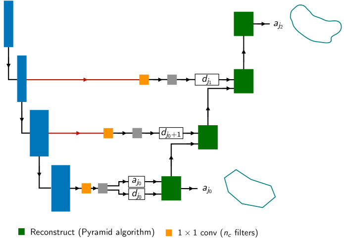
4.3.2 Architecture
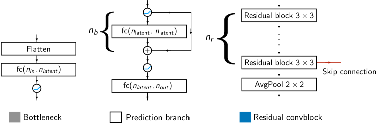
Our network is a hybrid analog of the U-Net. It consists of a two-dimensional convolutional encoder, a bottleneck of fully connected layers, and a one-dimensional decoder. The encoder and decoder are connected through skip-connections. The approximation and detail coefficients at the lowest resolution level are predicted in the bottleneck. Afterwards, the Pyramid Algorithm takes over to compute approximation coefficients at higher resolution levels (the decoder) using learnable wavelet filters. The needed detail coefficients at the higher resolution levels are predicted using the skip-connections. In practice, the detail coefficients are negligible on sufficiently high-resolution levels. For this reason, we only predict detail coefficients up to a prescribed level . The predictions at higher resolution levels are computed without detail coefficients. The full architecture is visualized in Figures 7 and 8. In addition, we provide a detailed summary below. The specific values for the architecture were determined using a hyperparameter search.
Encoder
The encoder consists of down-sampling blocks. Each block consists of (convolutional) residual blocks, using GELU-activation and kernels of size , followed by an average-pooling layer of size . The initial number of filters used in the first block is doubled after each other block. For example, if and the number of kernels at the first block is , then the subsequent blocks have , , , and , kernels, respectively.
Bottleneck
The encoder is followed by a bottleneck which consists of a stack of fully connected layers. The first layer in the bottleneck compresses the feature map from the encoder path to a feature map with channels using a convolution. Next, this compressed feature map is transformed to a vector in , where refers to the latent dimension of the MLP. Attached to this layer are four branches to predict the approximation and detail coefficients , respectively. Here corresponds to the spatial component of the contour. Each branch consists of fully-connected layers. The first layers map from to itself with GELU-activation and residual connections in between. The final layer transforms the -dimensional output to an element in .
Decoder
The detail coefficients at levels are predicted using skip-connections. For each skip-connection, we first compress the feature map from the encoder path to a feature map with channels using a convolution. Subsequently, two prediction branches, each having the same architecture as above, are used to predict the detail coefficients in (one for each spatial component). The predicted approximation coefficients at level and detail coefficients at levels are used as input to the Pyramid algorithm to reconstruct approximation coefficients up to level using learnable wavelet filters. The approximation coefficients at levels are reconstructed without detail coefficients.
Hyperparameters
The choices for the hyperparameters were based on a hyperparameter search, optimizing the Dice score. For the spleen and prostate we have set
respectively, and considered wavelet orders . Furthermore, for each order, we used the lowest possible resolution level and . In particular, for and for .
4.4 Optimization
In this section, we summarize the training procedure of our contouring-network. We use two different optimizers during training: one for the encoder and MLP (unconstrained), and one for the decoder (constrained wavelet network). The reason for this is that the needed step sizes on the non-trivial submanifold may significantly differ from those on the unconstrained (flat) parameter space. We use first order approximations of geodesics to perform SGD on the submanifold of constrained parameters, see Section 2.7.2. We remark that the generality of our framework allows for the computation of derivatives with respect to both the constrained and unconstrained parameters using normal automatic differentiation, see Algorithm 1.
We use plain SGD for the first eight epochs for both the constrained and unconstrained parameters. During this period the learning rate for the unconstrained parameters is linearly increased from to . The learning rate for the constrained parameters (wavelet filters) is linearly increased from to . After the initial warmup stage, we switch to the Adam optimizer for the unconstrained parameters. For both the constrained and unconstrained parameters, we use learning rate schedulers and decrease the learning rate by a factor 0.85 if no significant improvements in the validation loss are observed during the last ten epochs. We train all models for epochs using a batch size of and use the last epoch for inference. The computations were performed in PyTorch on a Geforce RTX Ti.
4.4.1 Loss
Next, we set up an appropriate loss to determine network parameters. To measure the discrepancy between the ground truth and the predicted curve, we define
This corresponds to the component-wise -error between the curves on resolution level with approximation coefficients and .
Notice that measures the discrepancy between observed and predicted curves on the highest resolution level only. We claim that this is sufficient for enforcing the approximation and detail coefficients at intermediate levels to agree as well. Indeed, recall the decomposition , which shows that any signal in can be uniquely written as a sum of elements in . Therefore, if two signals agree on , their associated approximation and detail coefficients on lower levels must agree as well.
4.4.2 Performance measures
We evaluate performance using the two-dimensional dice score, since our models are d and the hyperparameters were tuned to optimize this metric. We compute the dice score between curves using the implementation in shapely. This requires a polygonal approximation of the contour, which is directly obtained using the approximation coefficients at level .
For comparison, we also report the performance of a state-of-the-art baseline d-nnUNet [37]. We stress, however, that our objective, i.e., parameterizing contours, is different from the nnUNet’s objective. The binary ground truth matched by the 2d-nnUNet is a fundamentally different (often easier) object than the continuous representation of a curve matched by our networks. Subtle curvature and geometry may be accurately presented using our ground truth curves, e.g., by using a sufficiently large number of Fourier coefficients to compute approximation coefficients. Binary ground truth masks, however, cannot capture such subtle geometry due to their discrete nature.
4.5 Numerical results
| Model | Dice Spleen | Dice Prostate |
|---|---|---|
| nnunet | ||
| order | ||
| order | ||
| order | ||
| order | 7 | |
| order | ||
| order |
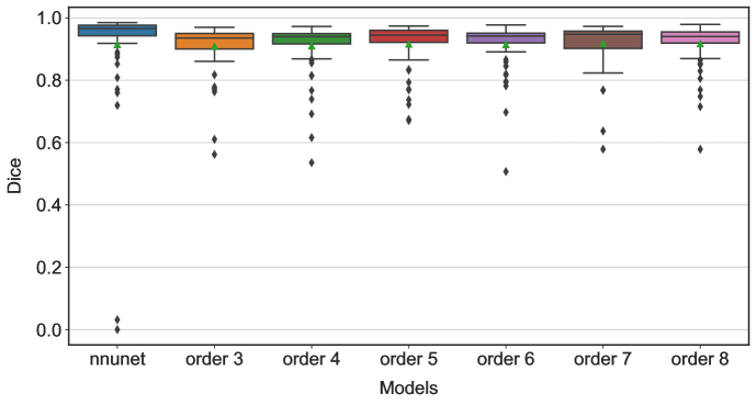
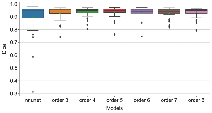
We have evaluated the performance of our wavelet networks for different orders on the unseen test data, see Table 2. Examples of predictions are depicted in Figure 10. For both the spleen and prostate, we observe that the best wavelet networks outperform the baseline in terms of dice score.
Spleen
The predictions of our wavelet models are accurate and on par with the baseline. The higher order wavelet models perform slightly better in terms of the mean dice score due to more outliers by the d-nnUNet. While the d-nnUNet has cases with higher dice scores, at the same time it has a relatively large number of outliers with relatively low dice scores. Our wavelet models, the best performing model in particular, are more robust in this sense, which is an especially important property for medical applications. The robustness is reflected in smaller standard deviations for the dice score, also see the boxplots in Figure LABEL:fig:boxplot_spleen. We have depicted examples of typical predictions in Figures LABEL:fig:138_spleen, LABEL:fig:144_spleen and LABEL:fig:362_spleen. These examples also showcase the fact that the ground truth curves may describe more subtle (complicated) geometry than binary masks. In Figures LABEL:fig:367_spleen and LABEL:fig:302_spleen we have depicted typical examples of predictions were our wavelet models struggle and the baseline performs better.
Prostate
The predictions of our wavelet models are accurate and outperform the baseline in terms of the dice score. We have depicted examples of typical predictions in Figures LABEL:fig:45_prostate, LABEL:fig:48_prostate and LABEL:fig:55_prostate. We observe, as for the spleen, that the wavelet models are more robust than the baseline, also see the box plots in Figure LABEL:fig:boxplot_prostate. In Figures LABEL:fig:13_prostate and LABEL:fig:5_prostate we show typical examples of where the wavelet models struggle to produce accurate predictions. In these examples, the predicted detail coefficients that correspond to parts of the curve with high curvature were not sufficiently accurate. The main reason for why we outperform the baseline is that it struggles with predicting “small” structures as in Figures LABEL:fig:45_prostate and LABEL:fig:5_prostate, often only correctly identifying a small number of pixels. It is in these cases where our contour models have a clear advantage; instead of annotating a few possibly disconnected set of pixels, our models have prior knowledge about the geometry and always predict a contour.
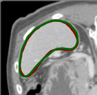
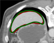
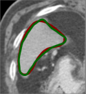
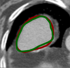
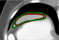
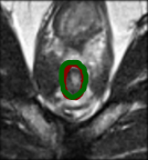
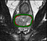
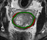
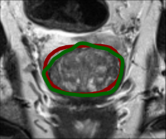
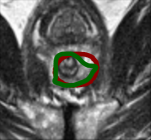
Task-optimized wavelets
We observe that the task-optimized wavelets differ significantly from the wavelets randomly initialized at the start of training. A comparison of an initial and task-optimized wavelet is depicted in Figure 11, see Appendix C.1 for more examples. We observed that in most cases, for both the prostate and spleen, the final wavelet appeared to be less “noisy” exhibiting less variation. In particular, the task-optimized wavelets for the spleen were much less noisy than for the prostate. We suspect, however, but did not test, that the wavelets for the prostate models would simplify if we increased the training time.
In numerical experiments we typically found different wavelets at the end of training for different initializations. One of the main reasons for this is that there is no unique “optimal wavelet” which solves the auto-contouring problem. Finally, as we increased the order of the wavelet filters, the final wavelets exhibited more oscillatory behavior and the number of zero-crossings increased. Our experiments did not reveal, however, a clear choice for a “best” order for our applications.
Non-degeneracy condition
In all numerical experiments the task-optimized filters satisfied the non-degeneracy condition of Theorem 3.14. We have illustrated this in Figure 12, where we observe (numerically), that the magnitudes of the final refinement masks are sufficiently far way from zero on . We have included more examples in Appendix C.2. We do note, however, that the initial wavelets were in some instances close to “degenerate”, in the sense came close to having a zero in , see Figures LABEL:fig:refinement_mask_init_0 and LABEL:fig:refinement_mask_init_1 for example. In all such cases, these “near-degeneracies” vanished quickly during the initial stages of training.
5 Conclusion
In this paper, we have introduced the CERM framework for imposing constraints on parametric models such as neural networks. The constraints are formulated as a finite system of equations. Under mild smoothness and non-degeneracy conditions, the parametric model can be made to obey the constraints exactly throughout the entire training procedure by performing SGD on a (possibly) curved space. As a major example, we have constructed a convolutional network whose filters are constrained to be wavelets. We have applied these wavelet networks to the prediction of boundaries of simply connected regions in medical images, where they outperform strong baselines.
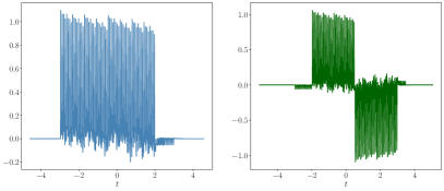
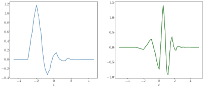
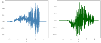
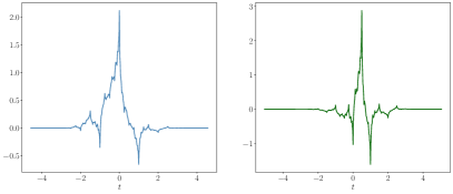
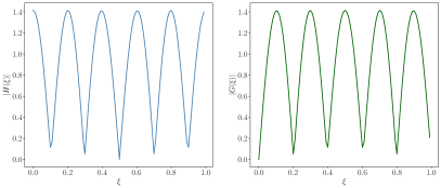
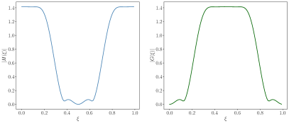
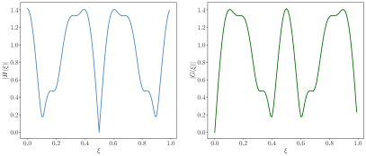
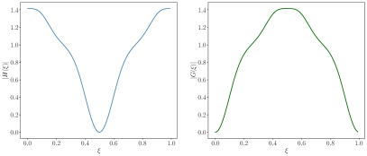
Acknowledgements
We thank Joren Brunekreef for his helpful feedback and discussions.
References
- [1] Diederik P. Kingma and Jimmy Lei Ba. Adam: A method for stochastic optimization. In 3rd International Conference on Learning Representations, ICLR 2015 - Conference Track Proceedings. International Conference on Learning Representations, ICLR, dec 2015.
- [2] Ilya Loshchilov and Frank Hutter. Decoupled weight decay regularization. arXiv preprint arXiv:1711.05101, 2017.
- [3] Ilya Loshchilov and Frank Hutter. Fixing weight decay regularization in adam, 2018.
- [4] Yang You, Jing Li, Sashank Reddi, Jonathan Hseu, Sanjiv Kumar, Srinadh Bhojanapalli, Xiaodan Song, James Demmel, Kurt Keutzer, and Cho-Jui Hsieh. Large batch optimization for deep learning: Training bert in 76 minutes. In International Conference on Learning Representations, 2020.
- [5] Yann LeCun, Yoshua Bengio, et al. Convolutional networks for images, speech, and time series. The handbook of brain theory and neural networks, 3361(10):1995, 1995.
- [6] Randall Balestriero and Yann LeCun. Police: Provably optimal linear constraint enforcement for deep neural networks, 2022.
- [7] Brandon Amos, Lei Xu, and J. Zico Kolter. Input convex neural networks. In Doina Precup and Yee Whye Teh, editors, Proceedings of the 34th International Conference on Machine Learning, volume 70 of Proceedings of Machine Learning Research, pages 146–155. PMLR, 06–11 Aug 2017.
- [8] Jack Richter-Powell, Yaron Lipman, and Ricky T. Q. Chen. Neural conservation laws: A divergence-free perspective, 2022.
- [9] Takeru Miyato, Toshiki Kataoka, Masanori Koyama, and Yuichi Yoshida. Spectral normalization for generative adversarial networks. In International Conference on Learning Representations, 2018.
- [10] Deepak Pathak, Philipp Krahenbuhl, and Trevor Darrell. Constrained convolutional neural networks for weakly supervised segmentation. In Proceedings of the IEEE international conference on computer vision, pages 1796–1804, 2015.
- [11] Michael M Bronstein, Joan Bruna, Taco Cohen, and Petar Veličković. Geometric deep learning: Grids, groups, graphs, geodesics, and gauges. arXiv preprint arXiv:2104.13478, 2021.
- [12] Maurice Weiler, Patrick Forré, Erik Verlinde, and Max Welling. Coordinate independent convolutional networks–isometry and gauge equivariant convolutions on riemannian manifolds. arXiv preprint arXiv:2106.06020, 2021.
- [13] Michael M Bronstein, Joan Bruna, Yann LeCun, Arthur Szlam, and Pierre Vandergheynst. Geometric deep learning: going beyond euclidean data. IEEE Signal Processing Magazine, 34(4):18–42, 2017.
- [14] Priya Donti, David Rolnick, and J Zico Kolter. Dc3: A learning method for optimization with hard constraints. In International Conference on Learning Representations, 2021.
- [15] Benedict Leimkuhler, Tiffany Vlaar, Timothée Pouchon, and Amos Storkey. Better training using weight-constrained stochastic dynamics. arXiv preprint arXiv:2106.10704, 2021.
- [16] Benedict Leimkuhler, Timothée Pouchon, Tiffany Vlaar, and Amos Storkey. Constraint-based regularization of neural networks. arXiv preprint arXiv:2006.10114, 2020.
- [17] Pablo Márquez-Neila, Mathieu Salzmann, and Pascal Fua. Imposing hard constraints on deep networks: Promises and limitations. arXiv preprint arXiv:1706.02025, 2017.
- [18] Soumava Kumar Roy, Zakaria Mhammedi, and Mehrtash Harandi. Geometry aware constrained optimization techniques for deep learning. In Proceedings of the IEEE Conference on Computer Vision and Pattern Recognition, pages 4460–4469, 2018.
- [19] Silvere Bonnabel. Stochastic gradient descent on riemannian manifolds. IEEE Transactions on Automatic Control, 58(9):2217–2229, 2013.
- [20] Hongyi Zhang, Sashank J. Reddi, and Suvrit Sra. Riemannian svrg: Fast stochastic optimization on riemannian manifolds. In D. Lee, M. Sugiyama, U. Luxburg, I. Guyon, and R. Garnett, editors, Advances in Neural Information Processing Systems, volume 29. Curran Associates, Inc., 2016.
- [21] Hiroyuki Kasai, Pratik Jawanpuria, and Bamdev Mishra. Riemannian adaptive stochastic gradient algorithms on matrix manifolds. In International Conference on Machine Learning, pages 3262–3271. PMLR, 2019.
- [22] Hiroyuki Sato, Hiroyuki Kasai, and Bamdev Mishra. Riemannian stochastic variance reduced gradient algorithm with retraction and vector transport. SIAM Journal on Optimization, 29(2):1444–1472, 2019.
- [23] Vladimir Vapnik. Principles of risk minimization for learning theory. Advances in neural information processing systems, 4, 1991.
- [24] Vladimir Vapnik. The nature of statistical learning theory. Springer science & business media, 1999.
- [25] Wei Hu, Lechao Xiao, and Jeffrey Pennington. Provable benefit of orthogonal initialization in optimizing deep linear networks. In International Conference on Learning Representations, 2020.
- [26] D.P. Bertsekas and W. Rheinboldt. Constrained Optimization and Lagrange Multiplier Methods. Computer science and applied mathematics. Elsevier Science, 2014.
- [27] John M Lee. Smooth manifolds. In Introduction to smooth manifolds. Springer, 2013.
- [28] John M Lee. Riemannian manifolds: an introduction to curvature, volume 176. Springer Science & Business Media, 2006.
- [29] Stephane Mallat. A Wavelet Tour of Signal Processing, Third Edition: The Sparse Way. Academic Press, Inc., USA, 3rd edition, 2008.
- [30] M.C. Pereyra and L.A. Ward. Harmonic Analysis: From Fourier to Wavelets. IAS/Park city mathematical subseries. American Mathematical Society, 2012.
- [31] L. Montefusco and L. Puccio. Wavelets: Theory, Algorithms, and Applications. ISSN. Elsevier Science, 2014.
- [32] M.W. Frazier. An Introduction to Wavelets Through Linear Algebra. Undergraduate Texts in Mathematics. Springer New York, 2001.
- [33] D.F. Walnut. An Introduction to Wavelet Analysis. Applied and Numerical Harmonic Analysis. Birkhäuser Boston, 2002.
- [34] P. Abry and P. Flandrin. On the initialization of the discrete wavelet transform algorithm. IEEE Signal Processing Letters, 1(2):32–34, 1994.
- [35] Cho-Chun Liu, Yaohui Liu, Zhengding Qiu, and Xiyu Du. On the initialization of the discrete wavelet transform algorithm. 1997 IEEE International Conference on Intelligent Processing Systems (Cat. No.97TH8335), 2:1220–1222 vol.2, 1997.
- [36] Michela Antonelli, Annika Reinke, Spyridon Bakas, Keyvan Farahani, Annette Kopp-Schneider, Bennett A Landman, Geert Litjens, Bjoern Menze, Olaf Ronneberger, Ronald M Summers, et al. The medical segmentation decathlon. Nature communications, 13(1):1–13, 2022.
- [37] Fabian Isensee, Paul F Jaeger, Simon AA Kohl, Jens Petersen, and Klaus H Maier-Hein. nnu-net: a self-configuring method for deep learning-based biomedical image segmentation. Nature methods, 18(2):203–211, 2021.
Appendix A Computing discrete convolutions using the DFT
In this appendix, we recall how to compute the two-sided convolution using the Discrete Fourier Transform (DFT). For this purpose, we first set up some terminology. Let be a -dimensional multi-index and let denote the space of two-sided -dimensional -valued sequences (or arrays) of order , i.e.,
The set is a vector space over of dimension . As usual, we will write for . Throughout this section inequalities involving multi-indices are interpreted component-wise. Similarly, we will denote the space of one-sided -dimensional -valued sequences or order by , i.e.,
Convolution and multiplication of polynomials
The two-sided convolution between sequences and is a new sequence defined by
Here we have omitted the ranges of and in the domain of summation to reduce clutter in the notation. It should be clear from the context, however, that and . Strictly speaking, we should incorporate and into the notation for as well. However, since we may always embed and into by padding with zeros, for any , leaving the result of convolution unchanged, we will ignore this distinction.
Convolutions can be efficiently computed using the DFT. To explain how to do so, we interpret and as the coefficients of Laurent polynomials and , respectively, where
The motivation for this interpretation is that the product has coefficients . We will exploit this relationship to compute the desired convolution. First, note that can be characterized by evaluating it on appropriately chosen points in . Here appropriate means that the evaluation operator mapping to the corresponding values of is an isomorphism on . Similarly, can be characterized by evaluation on appropriate points, and by evaluation on appropriate points, where . The key observation here is that if we fix appropriately chosen points in , we may go back and forth between value and coefficient representations of using the associated evaluation operator. Therefore, if the chosen evaluation operator and its inverse are analytically tractable, we can compute by evaluating .
The Discrete Fourier Transform
An appropriate choice for evaluation points is the roots of unity. The associated evaluation operator is the DFT, which is analytically tractable and computationally efficient. Here we shall consider the DFT from a purely algebraic point of view and mostly forget about its relation with Fourier Analysis. The interpretation we adopt is that the DFT evaluates (one-sided) multivariate polynomials on an “uniform discretization” of the -dimensional Torus . More precisely, for any , set and define for . We refer to as the -th order roots of unity. The -th order DFT is the map defined by
The DFT is an “appropriate” evaluation operator, i.e., it is an isomorphism. It characterizes the coefficients of a polynomial through evaluation at the roots of unity.
Evaluating Laurent-polynomials at the roots of unity
There is a slight difference between our objective, evaluating Laurent-polynomials, and the choice of evaluation operator (the DFT), which evaluates ordinary (one-sided) polynomials. In order to use the DFT for our purposes, we need to relate the evaluation of a Laurent polynomial at the roots of unity with the evaluation of an ordinary polynomial. This can be accomplished by exploiting the symmetry of the roots of unity.
Let and be arbitrary. Evaluation of the associated Laurent-polynomial at a root of unity yields
| (31) |
The right-hand side of (31) can be rewritten as a sum over positive indices only. Subsequently, we can exploit the symmetry of the roots of unity and recognize the result as evaluating a one-sided polynomial, i.e., as a DFT. More precisely, define by , where
Roughly speaking, the map places the components of with negative indices “after” the ones with positive indices. In numerical implementations, this operation is commonly referred to as a “fft shift”. This reordering can be used to recognize (31) as a DFT:
for . This shows that evaluation of at the roots of unity is equivalent to computing .
Convolution using the DFT
Finally, we explain how to compute the two-sided convolution . First, we characterize the coefficients of the Laurent-polynomial by evaluating it at the roots of unity . For this purpose, extend and to sequences in by padding with zeros. More formally, for each such that , define a padding operator by
Then evaluation of at the -th order roots of unity corresponds to computing
| (32) |
where denotes the Hadamard product. Since (32) is an equivalent representation of the Laurent-polynomial , which has coefficients , we conclude that
A.1 Periodic Convolutions
In certain applications, e.g., when dealing with wavelet expansions of periodic signals, one is given an array and wishes to compute , where is the -periodic extension of . This type of convolution is commonly referred to as periodic circular convolution. In particular, note that it suffices to compute for only, since is periodic as well. The periodic convolution can be efficiently computed using the DFT as well provided the periodicity has been appropriately taken into account. This is necessary to avoid boundary artifacts, see the explanation below.
First, observe that the sum
contains only a finite number of nonzero terms, since is finite. Furthermore, for , we do not need the full periodic extension of , but only a partial (finite) periodic extension . More precisely, define by for , where
Then for .
Finally, we apply the tools developed in the previous section to compute for using the DFT. More precisely, set
where , then
Appendix B Preprocessing
In this section we provide the details of our preprocessing steps.
B.1 Truncation Fourier coefficients
The magnitude of the approximated Fourier coefficients will typically stagnate and stay constant (approximately) beyond some critical order, since all computations are performed in finite (single) precision. We locate this critical order for each component , if present, by iteratively fitting the best line, in the least squares sense, through the points
We iterate this process until the residual is below a prescribed threshold . In practice, we set . The Fourier coefficients with index strictly larger than are set to zero.
B.2 Consistent parameterizations
To have consistent parameterizations we enforce that all contours start at angle zero at time zero relative to the midpoint of the region of interest . This is accomplished by exploiting the Fourier representation of . More precisely, let
be the initial contour with Fourier coefficients . The midpoint of the region enclosed by is given by
| (33) |
by Green’s Theorem. Here denotes the Lebesgue measure on and , are the Fourier coefficients of and its derivative, respectively.
We can now compute the desired parameterization by determining such that
and then use the shifted parameterization . While can be easily found using Newton’s method, it suffices in practice to simply re-order from the start, before computing the Fourier coefficients of . More precisely, we first define a shift of by
and then compute the Fourier coefficients of the resulting curve.
Appendix C Figures
C.1 Wavelets
In this section we show examples of initialized and task-optimized wavelets.
C.1.1 Spleen - first spatial component
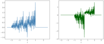
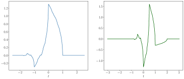
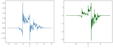
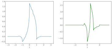

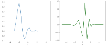
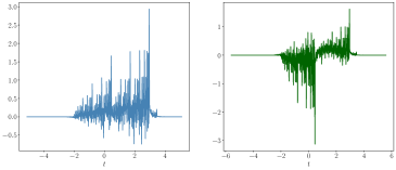
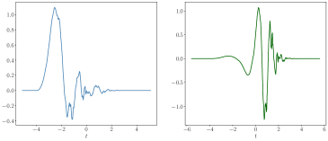
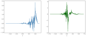
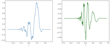
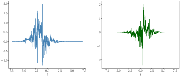
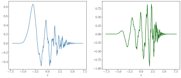
C.1.2 Spleen - second spatial component
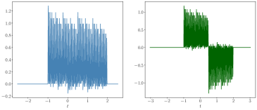
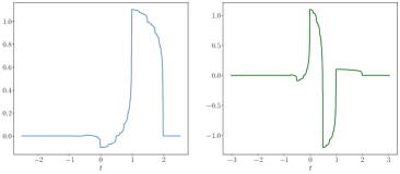
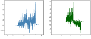
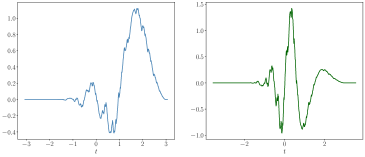

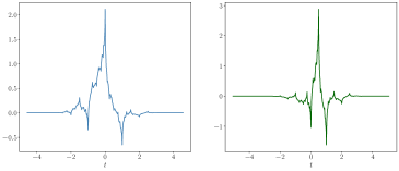
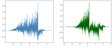
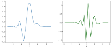
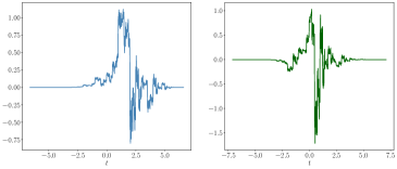
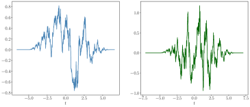
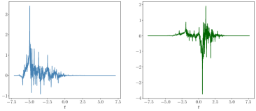
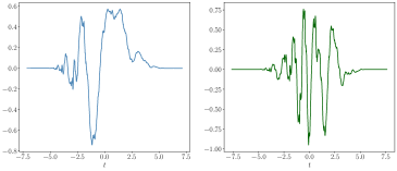
C.1.3 Prostate - first spatial component
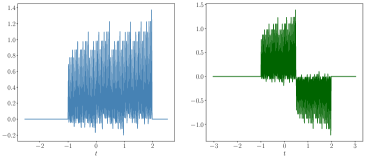
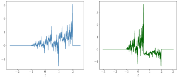
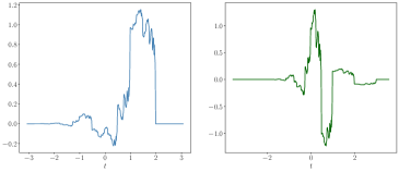
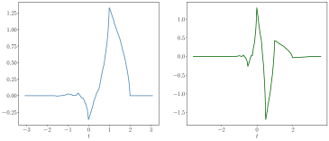
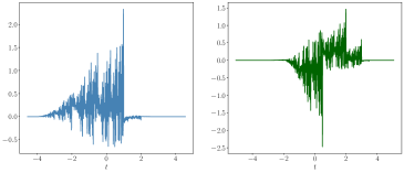
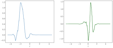
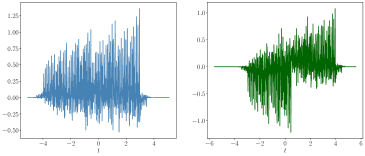
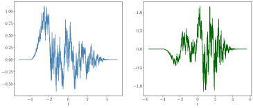
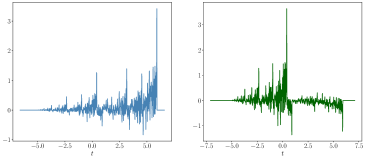
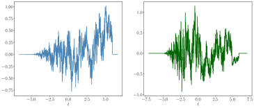
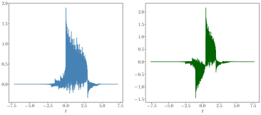
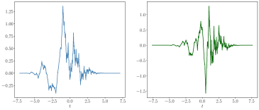
C.1.4 Prostate - second spatial component
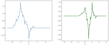
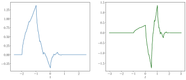
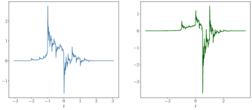
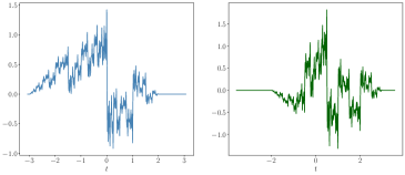
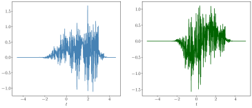
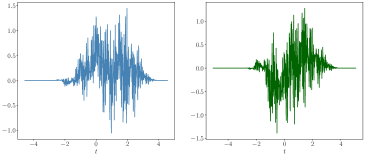
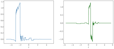
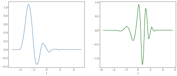
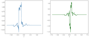
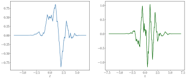
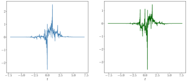
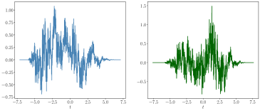
C.2 Refinement masks
In this section we visualize the refinement masks of the initial and task-optimized wavelets shown in the previous section.
C.2.1 Spleen - first spatial component
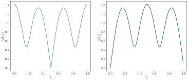

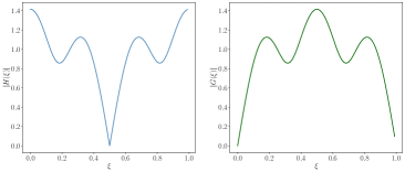
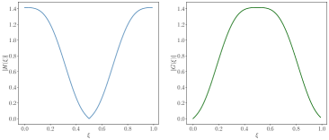
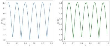
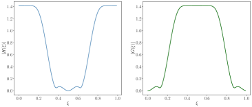
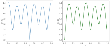
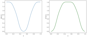
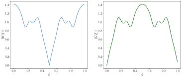
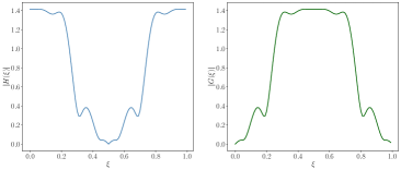
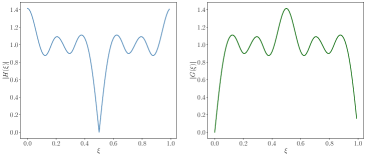
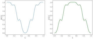
C.2.2 Spleen - second spatial component
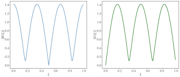
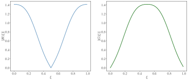
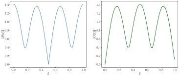
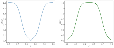
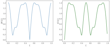
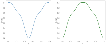
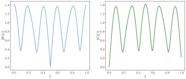
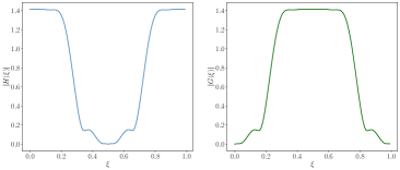
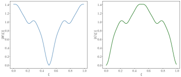
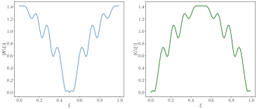
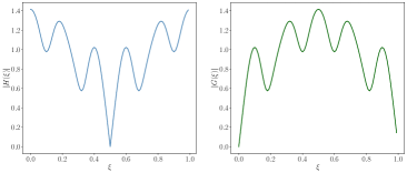
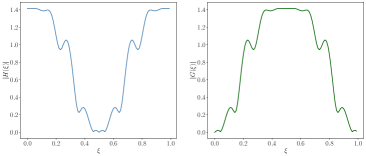
C.2.3 Prostate - first spatial component
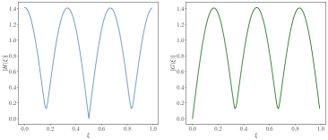
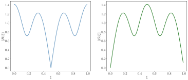
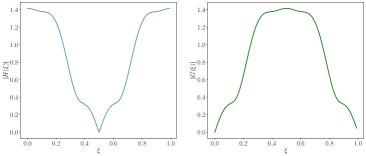
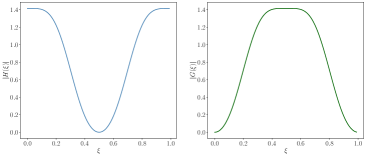
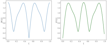
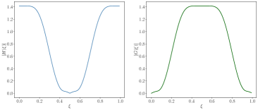
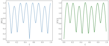
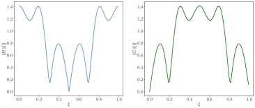
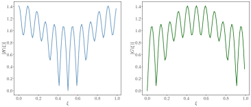
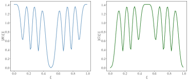
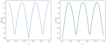
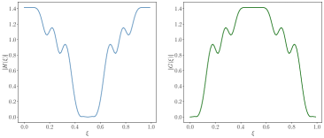
C.2.4 Prostate - second spatial component
