[]Corresponding author: Department of Mathematical Sciences, Universitetsparken 5, 2100 Copenhagen, Denmark. Email: wiuf@math.ku.dk
Evaluation of population structure inferred by principal component analysis or the admixture model
Abstract
Principal component analysis (PCA) is commonly used in genetics to infer and visualize population structure and admixture between populations. PCA is often interpreted in a way similar to inferred admixture proportions, where it is assumed that individuals belong to one of several possible populations or are admixed between these populations. We propose a new method to assess the statistical fit of PCA (interpreted as a model spanned by the top principal components) and to show that violations of the PCA assumptions affect the fit. Our method uses the chosen top principal components to predict the genotypes. By assessing the covariance (and the correlation) of the residuals (the differences between observed and predicted genotypes), we are able to detect violation of the model assumptions. Based on simulations and genome wide human data we show that our assessment of fit can be used to guide the interpretation of the data and to pinpoint individuals that are not well represented by the chosen principal components. Our method works equally on other similar models, such as the admixture model, where the mean of the data is represented by linear matrix decomposition.
keywords:
PCA; residuals; population modelling; ancient DNA; statistical fitxx xx, xxxx \accxx xx, xxxx
1 Introduction
Principal component analysis (PCA) and model-based clustering methods are popular ways to disentangle the ancestral genetic history of individuals and populations. One particular model, the admixture model (Pritchard et al., 2000), has played a prominent role because of its simple structure and, in some cases, easy interpretability. PCA is often seen as being model free but as noted by Engelhardt and Stephens (2010), the two approaches are very similar. The interpretation of the results of a PCA analysis is often based on assumptions similar to those of the admixture model, such that admixed individuals are linear combinations of the eigenvectors representing unadmixed individuals. In this way, the admixed individuals lie in-between the unadmixed individuals in a PCA plot. As shown for the admixture model, there are many demographic histories that can lead to the same result (Lawson et al., 2018a) and many demographic histories that violate the assumptions of the admixture model (Garcia-Erill and Albrechtsen, 2020). As we will show, this is also the case for PCA, since it has a similar underlying model (Engelhardt and Stephens, 2010).
The admixture model states that the genetic material from each individual is composed of contributions from distinct ancestral homogeneous populations. However, this is often contested in real data analysis, where the ancestral population structure might be much more complicated than that specified by the admixture model. For example, the ancestral populations might be heterogeneous themselves, the exact number of ancestral populations might be difficult to assess due to many smaller contributing populations, or the genetic composition of an individual might be the result of continuous migration or recent backcrossing, which also violates the assumptions of the admixture model. Furthermore, the admixture model assumes individuals are unrelated, which naturally might not be the case. This paper is concerned with assessing the fit of PCA building on the special relationship with the admixture model (Engelhardt and Stephens, 2010). In particular, we are interested in quantifying the model fit and assessing the validity of the model at the level of the sample as well as at the level of the individual. Using real and simulated data we show that the fit from a PCA analysis is affected by violations of the admixture model.
We consider genotype data from individuals and SNPs, such that is the number of reference alleles for individual and SNP . Typically, is assumed to be binomially distributed with parameter , where depends on the number of ancestral populations, , their admixture proportions and the ancestral population allele frequencies. For clustering based analysis such as ADMIXTURE (Alexander and Lange, 2011), is the number of clusters while in PCA, it is the top principal components. We give the specifics of the admixture model in the next section and show its relationship to PCA in the Material and methods section.
Several methods aim to estimate the best in some sense (Alexander and Lange, 2011; Evanno et al., 2005; Pritchard et al., 2000; Raj et al., 2014; Wang, 2019), but finding such does not imply the data fit the model (Lawson et al., 2018b; Janes et al., 2017). In statistics, it is standard to use residuals and distributional summaries of the residuals to assess model fit (Box et al., 2005). The residual of an observation is defined as the difference between the observed and the predicted value (estimated under some model). Visual trends in the residuals (for example, differences between populations) are indicative of model misfit, and large absolute values of the residuals are indicative of outliers (for example due to experimental errors, or kinship). If the model is correct, a histogram of the residuals is expected to be mono-modal centered around zero (Box et al., 2005).
In our context, Garcia-Erill and Albrechtsen (2020) argue that trends in the residual correlation matrix carries information about the underlying model and might be used for visual model evaluation. A method is designed to assess whether the correlation structure agrees with the proposed model, in particular, whether it agrees with the proposed number of homogeneous ancestral populations (Garcia-Erill and Albrechtsen, 2020). However, even in the case the model is correctly specified, the residuals are in general correlated (Box et al., 2005), and therefore, trends might be observed even if the model is true, leading to incorrect model assessment. To adjust for this correlation, a leave-one-out procedure, based on maximum likelihood estimation of the admixture model parameters, is developed that removes the correlation between residuals in the case the model is correct, but not if the model is misspecified (Garcia-Erill and Albrechtsen, 2020). This approach could also be applied to PCA, where expected genotypes could be calculated using probabilistic PCA (Meisner et al., 2021). This leave-one-out procedure is, however, computationally expensive.
To remedy the computational difficulties, we take a different approach to investigate the correlation structure. We suggest two different ways of calculating the correlation matrix of the residuals. The first is simply the empirical correlation matrix of the residuals. The second might be considered an estimated correlation matrix, based on a model. Both are simple to compute. Under mild regularity assumptions, these two measures agree if the model is correct and the number of SNPs is large. Hence, their difference is expected to be close to zero, when the admixture model is not violated. If the difference is considerably different from zero, then this is proof of model misfit.
To explore the adequacy of the proposed method, we investigate different ways to calculate the predicted values of the genotype (hence, the residuals), using Principal Component Analysis (PCA) in different ways. However, we also show that this approach can be used on estimated admixture proportions. Specifically, we use 1) an uncommon but very useful PCA approach (here, named PCA 1) based on unnormalized genotypes (Cabreros and Storey, 2019; Chen and Storey, 2015), 2) PCA applied to mean centred data (PCA 2), see Patterson et al. (2006), and 3) PCA applied to mean and variance normalised data (PCA 3) (Patterson et al., 2006). All three approaches are computationally fast and do not require separate estimation of ancestral allele frequencies and population proportions, as in Garcia-Erill and Albrechtsen (2020). Hence, the computation of the residuals are computationally inexpensive. Additionally, we show that this approach can also be applied to output from, for example, the software ADMIXTURE (Alexander et al., 2009) to estimate for each and , and to calculate the residuals from these estimates. An overview of PCA can be found in Jolliffe and Cadima (2016).
We demonstrate that our proposed method works well on simulated and real data, when the predicted values (and the residuals) are calculated in any of the four mentioned ways. Furthermore, we back this up mathematically by showing that the two correlation measures agree (if the number of SNPs is large) under the correct admixture model for PCA 1 and PCA 2. For the latter, a few additional assumptions are required. The estimated covariance (and correlation coefficient) under the proposed model might be seen as a correction term for population structure. Subtracting it from the empirical covariance, thus gives a covariance estimate with baseline zero under the correct model, independent of the population structure. It is natural to suspect that similar can be done in models with population structure and kinship, which we will pursue in a subsequent study.
In the next section, we describe the model, the statistical approach to compute the residuals, and how we evaluate model fit. In addition, we give mathematical statements that show how the method performs theoretically. In the ‘Results’ section, we provide analysis of simulated and real data, respectively. We end with a discussion. Mathematical proofs are collected in the appendix.
2 Materials and methods
2.1 Notation
For an matrix , denotes the -th column of , the -th row, the transpose matrix, and the rank. The Frobenius norm of a square matrix is
A square matrix is an orthogonal projection if and . A symmetric matrix has real eigenvalues (with multiplicity) and the eigenvectors can be chosen such that they are orthogonal to each other. If the matrix is positive (semi-)definite, then the eigenvalues are positive (non-negative).
For a random variable/vector/matrix , its expectation is denoted (provided it exist). The variance of a random variable is denoted , and covariance between two random variables is denoted (provided they exist). Similarly, for a random vector , the covariance matrix is denoted . For a sequence , of random variables/vectors/matrices, if as almost surely (convergence for all realisations but a set of zero probability), we leave out ‘almost surely’ and write as for convenience.
2.2 The PCA and the admixture model
We consider a model with genotype observations from individuals, and biallelic sites (SNPs), where is assumed to be (much) larger than , . The genotype of SNP in individual is assumed to be a binomial random variable
In matrix notation, we have with expectation , where and are dimensional matrices. Conditional on , we assume the entries of are independent random variables.
Furthermore, we assume the matrix takes the form , where is a (possibly unconstrained) matrix of rank , and is a (possibly unconstrained) matrix, also of rank (implying likewise is of rank , Lemma 13). Entry-wise, this amounts to
For the binomial assumption to make sense, we must require the entries of to be between zero and one.
In the literature, this model is typically encountered in the form of an admixture model with ancestral populations, see for example, Pritchard et al. (2000); Garcia-Erill and Albrechtsen (2020). The general unconstrained setting which applies to PCA has also been discussed (Cabreros and Storey, 2019). In the case of an admixture model, is a matrix of ancestral admixture proportions, such that the proportion of individual ’s genome originating from population is . Furthermore, is a matrix of ancestral SNP frequencies, such that the frequency of the reference allele of SNP in population is . In many applications, the columns of sum to one.
While we lean towards an interpretation in terms of ancestral population proportions and SNP frequencies, our approach does not enforce or assume the columns of (the admixture proportions) to sum to one, but allow these to be unconstrained. This is advantageous for at least two reasons. First, a proposed model might only contain the major ancestral populations, leaving out older or lesser defined populations. Hence, the sum of ancestral proportions might be smaller than one. Secondly, when fitting a model with fewer ancestral populations than the true model, one should only require the admixture proportions to sum to at most one.
2.3 The residuals
Our goal is to design a strategy to assess the hypothesis that is a product of two matrices. As we do not know the true , we suggest a number of ancestral populations and estimate the model parameters under this constraint. That is, we assume a model of the form
where each entry of follows a binomial distribution. has dimension , has dimension , and , hence also . Throughout, we use the index to indicate the imposed rank condition, and assume unless otherwise stated. The latter assumption is only to guarantee the mathematical validity of certain statements, and is not required for practical use of the method.
Our approach is build on the residuals, the difference between observed and predicted data. To define the residuals, we let be the orthogonal projection onto the -dimensional subspace spanned by the rows of (the true) , hence , and . Let be an estimate of based on the data , and assume is an orthogonal projection onto a -dimensional subspace. Later in this section, we show how an estimate can be obtained from an estimate of or an estimate of . Estimates of these parameters might be obtained using existing methods, based on for example, maximum likelihood analysis (Wang, 2003; Alexander et al., 2009; Garcia-Erill and Albrechtsen, 2020). Furthermore, for the three PCA approaches, an estimate of the projection matrix can simply be obtained from eigenvectors of a singular value decomposition (SVD) of the data matrix.
We define the matrix of residuals by
where is the observed data and , the predicted values. The latter might also be considered an estimate of , the expected value of . This definition of residuals is in line with how the residuals are defined in a multilinear regression model as the difference between the observed data (here, ) and the projection of the data onto the subspace spanned by the regressors (here, ). The essential difference being that in a multilinear regression model, the regressors are known and does not depend on the observed data, while is estimated from the data.
We assess the model fit by studying the correlation matrix of the residuals in two ways. First, we consider the empirical covariance matrix with entries
where
and the corresponding empirical correlation matrix with entries
. Secondly, we consider the estimated covariance matrix
with corresponding estimated correlation matrix,
. Here, is the diagonal matrix containing the average heterozygosities of each individual,
Under reasonable regularity conditions, we can quantify the behaviour of and as the number of SNPs become large. Specifically, we assume the rows of are independent and identically distributed with distribution , where denote the -dimensional mean vector of the distribution, and the -covariance matrix, that is,
. The matrix is assumed to be non-random, that is, fixed. These assumptions are standard and typically used in simulation of genetic data, see for example, Pickrell and Pritchard (2012); Cabreros and Storey (2019); Garcia-Erill and Albrechtsen (2020). Often is taken to be the product of independent uniform distributions in which case and is a diagonal matrix with entries , though other choices have been applied, see for example Balding and Nichols (1995); Conomos et al. (2016).
Let be the diagonal matrix with entries
| (1) |
It follows from Lemma 7 in the appendix, that converges to as . Furthermore, as is the variance of (it is binomial), then might be considered an estimate of this variance. The proofs of the statements are in the appendix.
Theorem 1.
Let . Under the given assumptions, suppose further that as , for some matrix . Then, is an orthogonal projection. Furthermore, the following holds,
as . Hence, also
as . For , if , then the right hand side is the zero matrix, whereas this is not the case in general for .
Theorem 2.
Assume and . Furthermore, suppose as in Theorem 1 and that the vector with all entries equal to one is in the space spanned by the rows of (this is, for example, the case if the admixture proportions sum to one for each individual). Then,
| (2) |
In addition, if takes the form
where has dimension , and , then (2) holds for each component of individuals. If , then
for all individuals in the -th component, irrespective the form of , .
Theorem 3.
Assume and . Furthermore, suppose as in Theorem 1 and that takes the form
where has dimension , . Then, converges as to a value larger than or equal to for all .
The same statements in the last two theorems hold with and replaced by and , respectively.
The three theorems provide means to evaluate the model. In particular, Theorem 1 might be used to assess the correctness (or appropriateness) of the proposed , while Theorem 2 and Theorem 3 might be used to assess whether data from a group of individuals (e.g., a modern day population) originates from a single ancestral population, irrespective, the origin of the remaining individuals. We give examples in the Results section.
The work flow is shown in Algorithm 1. We process real and simulated genotype data using PCA 1, PCA 2, PCA 3, and the software ADMIXTURE, and evaluate the fit of the model.
-
1.
Choose ,
-
2.
Compute an estimate of the projection ,
-
3.
Calculate the residuals ,
-
4.
Calculate the correlation coefficients, and ,
-
5.
Plot and the difference, the corrected correlation coefficients, ,
-
6.
Assess visually the fit of the model.
2.4 Estimation of
Estimation of and has received considerable interest in the literature, using for example, maximum likelihood (Wang, 2003; Alexander et al., 2009), Bayesian approaches (Pritchard et al., 2000) or PCA (Engelhardt and Stephens, 2010).
We discuss different ways to obtain an estimate of .
2.4.1 Using an estimate of
An estimate might be obtained by projecting onto the subspace spanned by the rows of ,
assuming for the calculation to be valid.
We apply this approach to estimate the projection matrix using output from the software ADMIXTURE.
2.4.2 Using an estimate of
Let be linearly independent rows chosen from (out of rows). Then, an estimate of is
assuming for the calculation to be valid. Alternatively, one might apply the Gram-Schmidt method in which case the vectors are orthonormal by construction and . The estimate is independent of the choice of the rows, provided .
2.4.3 Using PCA 1
We consider a PCA approach, originally due to Chen and Storey (2015), to estimate the space spanned by the rows of . We follow the procedure laid out in Cabreros and Storey (2019).
Let be the symmetric matrix
Since is symmetric, all eigenvalues are real and the matrix is diagonalisable. Furthermore, is a variance adjusted version of , see (1). Let be orthogonal eigenvectors belonging to the largest eigenvalues of , counted with multiplicities. Define the matrix and the orthogonal projection matrix
onto the subspace given by the span of the vectors .
In this particular case, convergence of can be made precise. Define the matrix . Then, is symmetric and positive semi-definite because and both are positive semi-definite. Hence, has non-negative eigenvalues. Furthermore, according to Lemma 8 in the appendix, converges to as .
Theorem 4.
Assume . Let be the eigenvalues of , with corresponding orthogonal eigenvectors . In particular, , as has rank . Let be the orthogonal projection onto the span of , that is,
where .
Assume or , referred to as the eigenvalue condition. Then, as . If the eigenvalue condition is fulfilled for , then , that is, is the orthogonal projection onto the span of the row vectors of . In particular, the eigenvalue condition is fulfilled for if and only if is positive definite. The latter is the case if is positive definite.
For , the correct row space of is found eventually, but not itself. If , then a subspace of this row space is found, corresponding to the largest eigenvalues. As the data is not mean centred, we discard the first principal component, and use the subsequent eigenvectors and eigenvalues.
2.4.4 Using PCA 2 (mean centred data)
A popular approach to estimation of in the admixture model is PCA based on mean centred data, or mean and variance normalised data (Pritchard et al., 2000; Engelhardt and Stephens, 2010; Patterson et al., 2006).
Let be the SNP-wise mean centred genotypes, where is an matrix with all entries equal to one. Following the exposition and notation in Cabreros and Storey (2019), let be the SVD of , where consists of the row-wise principal components of , ordered according to the singular values. Define
where is a vector with all entries one, and contains the top rows of . Then, an estimate of the projection is
The squared singular values in the SVD decomposition of are the same as the eigenvalues of
(Jolliffe, 2002). We have
| (3) |
Let denote the right hand side of (3).
Theorem 5.
Let be the eigenvalues of , with corresponding orthogonal eigenvectors . In particular, and . If has all diagonal entries positive, then .
Let and let be the orthogonal projection onto the span of , that is,
where . If or , then as .
There are no guarantees that for , we have and that the difference between and converges to zero for large . However, this is the case under some extra conditions, and appears to be the case in many practical situations, see the Results section.
2.4.5 Using PCA 3 (mean and variance normalised data)
Let be the SNP mean and variance normalised genotypes, where is an diagonal matrix with -th entry being the observed standard deviation of the genotypes of SNP . All SNPs for which no variation are observed are removed, hence the number of SNPs might be smaller than the original number, . Following the same procedure as for PCA 2, let be the SVD of , where consists of the row-wise principal components of , ordered according to the singular values. Define
where , and contains the top rows of . Then, an estimate of the projection is
We are not aware of any theoretical justification of this procedure similar to Theorem 1, but it appears to perform well in many practical situations, according to our simulations.
2.5 Simulation of genotype data
We simulated genotype data from different demographic scenarios using different sampling strategies. We deliberately choose different sampling strategies to challenge the method. We first made simple simulations that illustrate the problem of model fit as well as to demonstrate the theoretical and practical properties of the residual correlations that arise from having data from a finite number of individuals and a large number of SNPs. An overview of the simulations are given in Table 1.
In the first two scenarios, the ancestral allele frequencies are simulated independently for each ancestral population from a uniform distribution, for each site and each ancestral population . In scenario 1, we simulated unadmixed individuals from three populations with either an equal or an unequal number of sampled individuals from each population. In scenario 2, we simulated two ancestral populations and a population that is admixed with half of its ancestry coming from each of the two ancestral populations.
In scenario 3, we set and simulated spatial admixture in a way that resembles a spatial decline of continuous gene flow between populations living in a long narrow island. We first simulated a single population in the middle of the long island. From both sides of the island, we then recursively simulated new populations from a Balding-Nichols distribution with parameter using the R package ‘bnpsd’ (Ochoa and Storey, 2019). In this way, each pair of adjacent populations along the island has an of 0.001. Additional details on the simulation and an schematic visualization can be found in Figure 2 of Garcia-Erill and Albrechtsen (2020).
In scenario 4, we first simulated allele frequencies for an ancestral population from a symmetric beta distribution with shape parameter 0.03, , which results in an allele frequency spectrum enriched for rare variants, mimicking the human allele frequency spectrum. We then sampled allele frequencies from a bifurcating tree (((pop1:0.1,popGhost:0.2):0.05,pop2:0.3):0.1,pop3:0.5), where pop1 and popGhost are sister populations and pop3 is an outgroup. Using the Balding-Nichols distribution and the branch lengths of the tree (see Figure 5), we sampled allele frequencies in the four leaf nodes. Then, we created an admixed population with 30% ancestry from popGhost and 70% from pop2. We sampled 10 million genotypes for 50 individuals from each population except for the ghost population which was not included in the analysis, and subsequently removed sites with a sample minor allele frequency below 0.05, resulting in a total of 694,285 sites.
In scenario 5, we simulated an ancestral population with allele frequencies from a uniform distribution Unif , from which we sampled allele frequencies for two daughter populations from a Balding Nicholds distributions with from the ancestral population, using ’bnpsd’. We then created recent hybrids based on a pedigree where all but one founder has ancestry from the first population. The number of generations in the pedigree then determines the admixture proportions and the age of the admixture where F1 individuals have one unadmixed parent from each population and backcross individuals have one unadmixed parent and the other F1. Double backcross individuals have one unadmixed parent and the other is a backcross. We continue to quadruple backcross with one unadmixed parent and the other triple backcross. Note that for the recent hybrids the ancestry of the pair of alleles at each loci is no longer independent which is a violation of the admixture model.
| Scenario | Description | 111Ancestral allele frequencies, | |||
|---|---|---|---|---|---|
| 1 | 3 | 20,20,20 | Unadmixed | ||
| 1 | 3 | 10,20,30 | Unadmixed | ||
| 2 | 2 | 20,20,20 | Admixed | ||
| 2 | 2 | 10,20,30 | Admixed | ||
| 3 | 500 | 222after applying MAF% filtering, 88,082 remained. | Spatial with | ||
| between adjacent populations | |||||
| 4 | 4 | 50,50,50,50,0333No reference samples are provided on the ghost population. | 444after applying MAF% filtering, 694,285 remained. | Ghost admixture | |
| 5 | 2 | 20,20,50 | Recent hybrids |
3 Results
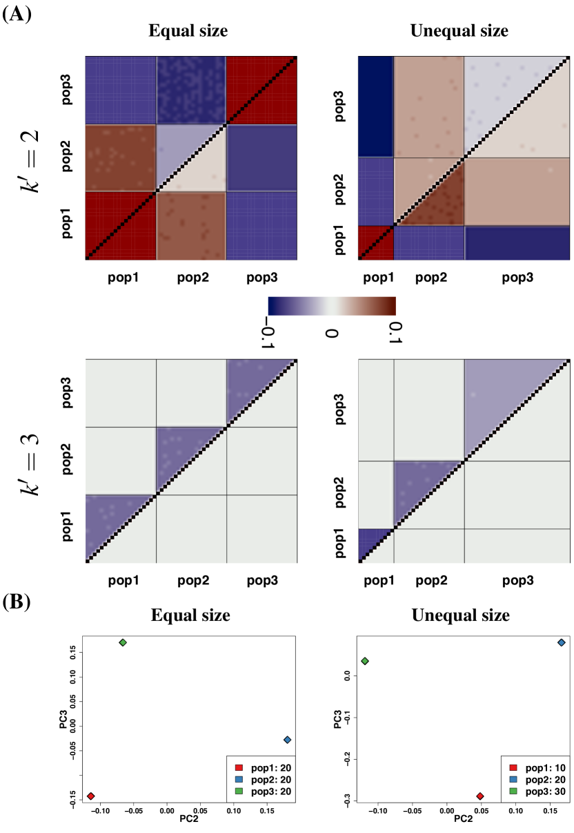
3.1 Scenario 1
In this first set-up, we demonstrate the method using PCA 1 only. We simulated unadmixed individuals from ancestral populations
where is a row vector with all elements being one, and . We simulated genotypes for individuals with sample sizes and , respectively, as detailed in the previous section. In Figure 1(A), we show the residual correlation coefficients for and plot the corresponding major PCs. For the PCA 1 approach, the first principal component does not relate to population structure as the data is not mean centered, and we use the following principal components.
When assuming that there are only two populations, , we note that the empirical correlation coefficients appear largely consistent within each population sample, but the corrected correlation coefficients are generally non-zero with different signs, which points to model misfit. In contrast, when assuming the correct number of populations is , the empirical correlation coefficients match nicely the theoretical values of , which comply with Theorem 2 (see Table 2). A fairly homogeneous pattern in the corrected correlation coefficients appears around zero across all samples. This is a good indication that the model fits well and that the PCA plots using principal components 2 and 3 reflex the data well.
| Scenario 1 | pop1 | pop2 | pop3 | ||||
| 555The second line of in each case shows the theoretical value obtained from the limit in Theorem 1. | -0.0526 (0.0015) | -0.0526 (0.0016) | -0.0526 (0.0016) | ||||
| -0.0526 | -0.0526 | -0.0526 | |||||
| 0e-04 (0.0015) | 0e-04 (0.0016) | 0e-04 (0.0016) | |||||
| -0.1111 (0.0011) | -0.0526 (0.0016) | -0.0345 (0.0016) | |||||
| -0.1111 | -0.0526 | -0.0345 | |||||
| 0e-04 (0.0012) | 0e-04 (0.0016) | 0e-04 (0.0016) | |||||
| Scenario 2 | pop1 | admixed | pop3 | ||||
| -0.0419 (0.0015) | -0.0192 (0.0015) | -0.0420 (0.0015) | |||||
| -0.0420 | -0.0193 | -0.0420 | |||||
| 0e-04 (0.0015) | 0e-04 (0.0015) | 0e-04 (0.0015) | |||||
| -0.0701 (0.0018) | -0.0228 (0.0014) | -0.0304 (0.0016) | |||||
| -0.0701 | -0.0229 | -0.0304 | |||||
| 0e-04 (0.0017) | 0e-04 (0.0014) | 0e-04 (0.0016) | |||||
| Scenario 4 | pop1 | pop2 | pop3 | pop4 | |||
| -0.0190 (0.0015) | 0.0027 (0.0015) | -0.0204 (0.0017) | 0.0122 (0.0013) | ||||
| 0.0009 (0.0015) | 0.0147 (0.0015) | 0e-04 (0.0017) | 0.0208 (0.0013) | ||||
| -0.0204 (0.0015) | -0.0204 (0.0015) | -0.0204 (0.0017) | -0.0204 (0.0014) | ||||
| 0e-04 (0.0015) | 0e-04 (0.0015) | 0e-04 (0.0017) | 0e-04 (0.0013) |
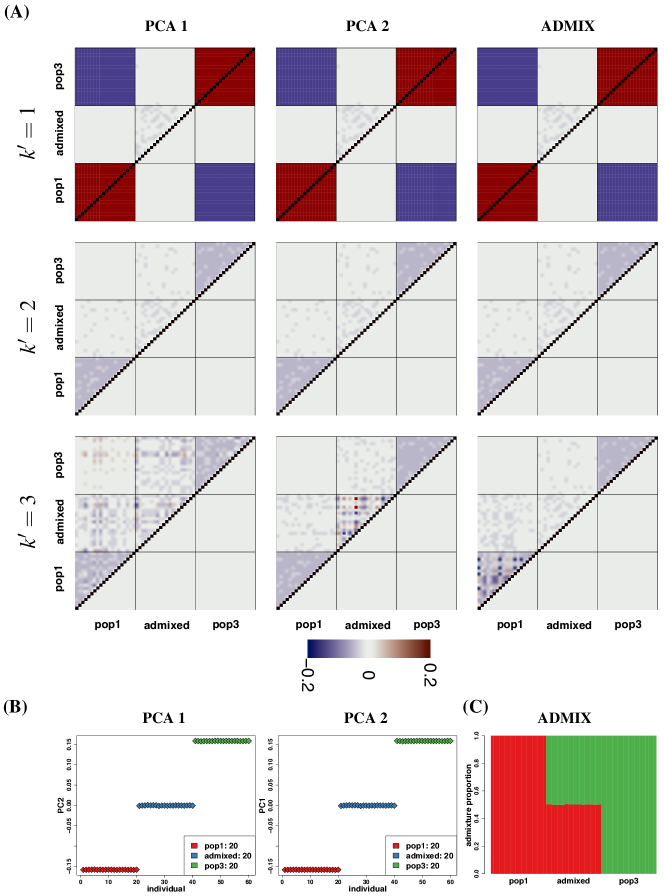
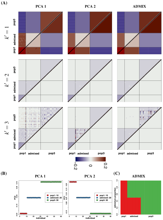
3.2 Scenario 2
In this set-up we also include admixed individuals. We simulated samples from two ancestral populations and individuals that are a mix of the two. We then applied all three PCA procedures and the software ADMIXTURE to the data. Specifically, we choose
with true ancestral populations, and or , see the previous section for details. We analysed the data with , and obtained the correlation structure shown in Figures 2 and 3, and Table 2. The two standard approaches PCA 2 and PCA 3 show almost identical results, hence only PCA 2 is shown in the figures. Both PCA 2 and PCA 3 use the top principal components, while PCA 1 disregards the first, hence the discrepancy in the axis labeling in Figures 2(b) and 3/b). For none of the principal components are used and the predicted normalized genotypes is simply 0. All four methods show consistent results, in particular, for the correct (), while there are smaller discrepancies between the methods for wrong . This is most pronounced for PCA 1 and ADMIXTURE. We note that the average correlation coefficient of within each population sample comply with Theorem 1 (see Table 2). A fairly homogeneous pattern in the corrected correlation coefficients appears around zero across all samples for , as in scenario 1, which shows that the model fits well. However, unlike in scenario 1 the bias for the empirical correlation coefficient is not a simple function of the sample size (see Table 2).
In this case, and similarly in all other investigated cases, we don’t find any big discrepancies between the four methods. Therefore, we only show the results of PCA 1 for which we have theoretical justification for the results.
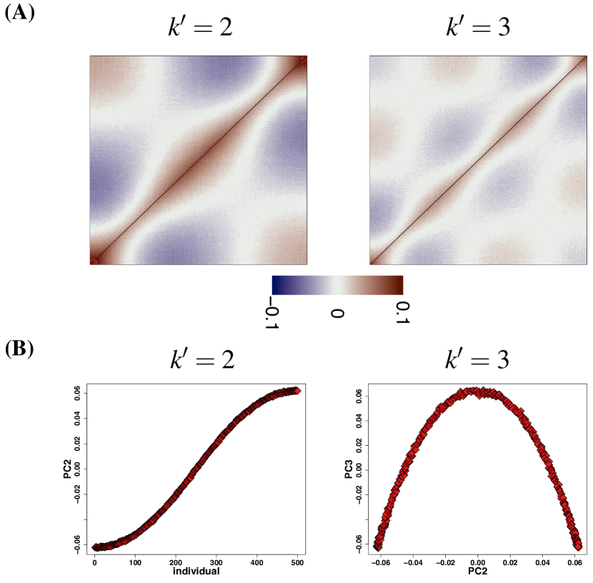
3.3 Scenario 3
We simulated genotypes for individuals at sites with continuous genetic flow between individuals, thus there is not a true . We analysed the data assuming , see Figure 4. In the figure, the individuals are ordered according to the estimated proportions of the ancestral populations, hence it appears there is a color wave pattern in the empirical and the corrected correlation coefficients, see Figure 4(A). As expected, the corrected correlation coefficients are closer to zero for than , though the deviations from zero are still large. We thus find no support for the model for either value of . This is consistent with the plots of the major PCs, that show continuous change without grouping the data into two or three clusters, see Figure 4(B).
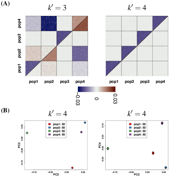
3.4 Scenario 4
This case is based on the tree in Figure 5, which include an unsampled (so-called) ghost population, popGhost. The popGhost is sister population to pop1.

We simulated genotypes for individuals: 150 unadmixed samples from pop1, pop2, and pop3; and 50 samples admixed with 0.3 ancestry from popGhost and 0.7 ancestry from pop2 (as pop4), as detailed in the previous section. As there is drift between the populations and hence genetic differences, the correct (pop1, pop2, pop3, popGhost). This is picked up by our method that clearly shows is wrong with large deviation from zero in the corrected correlation coefficients. In contrast, for , the corrected correlation coefficients are almost zero (Figure 6).
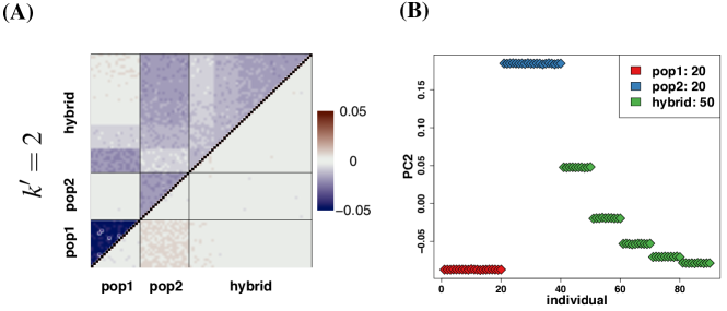
3.5 Scenario 5
In the last example, we simulated two populations (originating from a common ancestral population) and created admixed populations by backcrossing, as detailed in the previous section. Thus, the model does not fulfil the assumptions of the admixture model in that the number of reference alleles are not binomially distributed, but depends on the particular backcross and the frequencies of the parental populations.
We simulate genotypes for individuals at sites. There are 20 homogeneous individuals from each parental population, and 10 different individuals from each of the different recent admixture classes. Then, we analysed the data with and found the corrected correlation coefficients deviated consistently from zero, in particular for one of the parental populations (Figure 7). We are thus able to say the admixture model does not provide a reasonable fit.
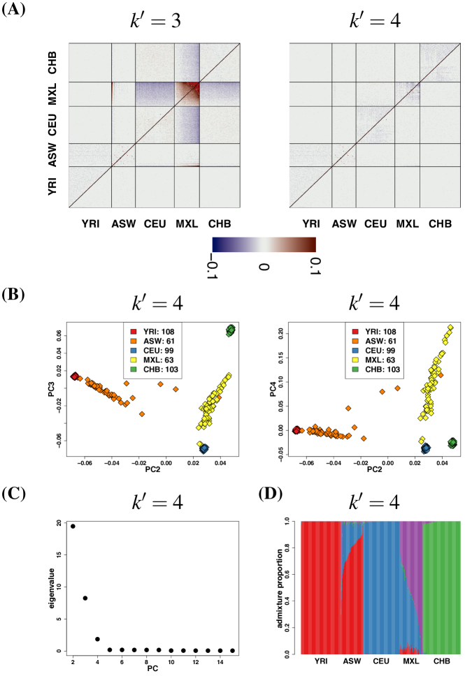
3.6 Real data
We analysed a whole genome sequencing data set from the 1000 Genomes Project (Auton et al., 2015), see also Garcia-Erill and Albrechtsen (2020) where the same data is used. It consists of data from five groups of different descent: a Yoruba group from Ibadan, Nigeria (YRI), residents from Southwest US with African ancestry (ASW), Utah residents with Northern and Western European ancestry (CEU), a group with Mexican ancestry from Los Angeles, California (MXL), and a group of Han Chinese from Beijing, China (CHB) with sample sizes and , respectively, in total, . We kept only sites present in the Human Origins SNP panel (Lazaridis et al., 2014), with a total of SNPs were left after a MAF filter of 0.05.
We analyzed the data with . For , Figure 8 shows that it is not possible to explain the relationship between MXL, CEU and CHB, indicating that MXL is not well explained as a mixture of the two. For , the color shades of the corrected correlation coefficients are almost negligible within each population, pointing at a contribution from a native american population. This is further corroborated in Figure 8(D) that shows estimated proportions from the four ancestral populations using the software ADMIXTURE.
4 Discussion
We have developed a novel approach to assess model fit of PCA and the admixture model based on structure of the residual correlation matrix. We have shown that it performs well for simulated and real data, using a suit of different PCA methods, commonly used in the literature, and the ADMIXTURE software to estimate model parameters. By assessing the residual correlation structure visually, one is able to detect model misfit and violation of modelling assumptions.
The model fit is assessed by comparing visually two matrices of residual correlation coefficients. The theoretical and practical advantage of our approach lie in three aspects. First, our approach is computationally simple and fast. Calculation of the two residual correlation matrices and their difference is computationally inexpensive. Secondly, our approach provides a unified approach to model fitting based on PCA and clustering methods (like ADMIXTURE). In particular, it provides simple means to assess the adequacy of the chosen number of top principal components to describe the structure of the data. Assessing the adequacy by plotting the principal components against each other might lead to false confidence. In contrast, our approach exposes model misfit by plotting the difference between two matrices of the residual correlation coefficients. Thirdly, it comes with theoretical guarantees in some cases. These guarantees are further back up by simulations in cases, we cannot provide theoretical validity. Finally, our approach might be adapted to work on NGS data without estimating genotypes first, but working directly on genotype likelihoods.
Data availability
The data sets used in this study are all publicly available, including simulated and real data. Information about the R code used to analyze and simulate data is available at https://github.com/Ginwaitthreebody/evalPCA. The variant calls for the 1000 Genomes Project data used are publicly available at ftp://ftp.1000genomes.ebi.ac.uk/vol1/ftp/release/20130502/.
Acknowledgements
The authors are supported by the Independent Research Fund Denmark (grant number: 8021-00360B) and the University of Copenhagen through the Data+ initiative. SL acknowledges the financial support from the funding agency of China Scholarship Council. GGE and AA are supported by the Independent Research Fund Denmark (grant numbers: 8049-00098B and DFF-0135-00211B respectively).
Appendix A
We first state the expectation and covariance matrix of and , respectively, under the given distributional assumptions,
for , where
and
The unconditional columns , , of are independent random vectors by construction.
The above implies that
| (4) |
Auxiliary results are in appendix B.
Lemma 7.
The estimator is an unbiased estimator of , that is, . Furthermore, it holds that as .
Proof.
Conditional on , using binomiality, we have , and the first result follows. For convergence, note that , , unconditionally, form a sequence of iid random variables with finite variance, hence the convergence statement follows from the strong Law of Large Numbers (Jacod and Protter, 2004). ∎
Lemma 8.
The estimator is an unbiased estimator of , that is, . Furthermore, it holds that as , and
Proof.
Unbiasedness follows from (4) and Lemma 7. Consider the -th entry of , namely, . The sequence , , is iid with finite variance, hence converges to as by the strong Law of Large Numbers (Jacod and Protter, 2004). Combined with Lemma 7 gives convergence of to as .
It remains to prove the inequality. Define
Then,
Using , independence of and for , and , we have
which proves the claim. ∎
The convergence result is also in Chen and Storey (2015, theorem 2). The second part provides the rate of convergence of in the -norm. Convergence is contingent on large , rather than large , and requires to increase at least like the square of .
Proof of Theorem 1. Since is assumed to be an orthogonal projection, that is, and , then also the limit is an orthogonal projection, and .
Consider the empirical covariance . Define the variables with replaced by , and the empirical covariance
defined similarly to , with The sequences , , and , , are iid random variables, by the distributional assumptions on . Furthermore, since is an orthogonal projection, then is bounded (Lemma 12). Therefore, also is bounded uniformly in by .
Using boundedness, independence and the strong Law of Large Numbers (Jacod and Protter, 2004),
| (5) |
for , and The latter equality follows from (4).
Consider . Hence,
as by assumption of the theorem. It follows that converges to as . Furthermore,
The absolute value of the first term in the last line above is bounded by
and similarly for the second term. The third is bounded by
All three terms converge to zero as , hence we conclude from (5) that as .
The result for the estimated covariance follows from convergence of and by assumption of the theorem. The remaining part follows from the convergence of and . Note that , hence the second equation holds. The last statement of the theorem follows directly.
Proof of Theorem 2. Consider , where is the projection onto the row space of . Then, contains the residuals under multiple regression of the rows of on the rows of (Box et al., 2005). Since is in the row space of , then the sum of the residuals is zero for each : (the assumption that is in the row space is equivalent to having an intercept in the regression model) (Box et al., 2005). We have, for ,
since the distribution of is independent of . From the proof of Theorem 4, it follows that converges to as . Hence,
and the desired result follows by rearrangement.
If takes the given form, then the residuals under multiple regression are independent between compartments, as the projection is
where has dimension . It follows that the computation above holds for each compartment. Finally, if , then the distribution of the random vector is exchangeable, resulting in
assuming the individuals in the -th compartment are numbered to . Rearranging terms and substituting for the moments of yields the desired result.
Proof of Theorem 3. Consider , where is the projection onto the row space of . If , then the distribution of the random variables are exchangeable, resulting in
Rearranging terms and substituting for the moments of yields the desired result.
Proof of Theorem 4. The convergence statement of the theorem is a special case of Theorem 9 in Appendix B. Take (that depends on the number of SNPs , and the particular realization), , and in the theorem ( is used as a generic index in Theorem 9). Then, and , and the conclusion of Theorem 4 holds. Convergence in Frobenius norm is equivalent to pointwise convergence (as is fixed) as by definition.
If is positive definite, then it has rank . As by assumption, it follows from Lemma 13 that . Consequently, there are positive eigenvalues of and , and the eigenvalue condition holds. Conversely, assume the eigenvalue condition holds. By definition . As by assumption, then also and we conclude . It follows that the rank of is ; consequently, it is positive definite.
If , then and (as ), and . So assume . Since the eigenvalue condition is fulfilled, then from the above, we have , and Lemma 13 yields that the row space of and agree. Similarly, we have and Lemma 13 yields that the row space of and agree. This implies the row space of and agree. Consequently, , and the statement holds.
Proof of Theorem 5. It follows trivially that is an eigenvector of with eigenvalue . If has all entries positive, then it is positive definite and is also positive definite, hence has rank . It follows from Lemma 13 that has rank , hence .
Similarly to the proof of Lemma 8 in Appendix B, one can show and as , where denotes the right hand side of (3). The remaining part of the theorem is proven similarly to Theorem 4.
Proof of Theorem 6. Note that is an eigenvector of with eigenvalue . Consider an eigenvector of , orthogonal to with eigenvalue . Then, the following two equations are equivalent,
| (6) |
where it is used that and . It shows that is an eigenvector of with eigenvalue . Since has rank and the vector is in the space spanned by the rows of , then has rank . It follows that there are at most positive eigenvalues of , that is, at most eigenvalues of such that . Furthermore, there are precisely positive eigenvalues, provided is positive definite (Lemma 13). The remaining eigenvalues of are zero, that is, the corresponding eigenvalues of are .
Assume is positive definite, then by the above argument there precisely are eigenvalues of such that with corresponding orthogonal eigenvectors . It follows from (6) that are in the space spanned by the rows of , hence the eigenvectors are in the space spanned by the rows of . By assumption is also in that row span. Hence, forms an orthogonal basis of the row span of , as has rank . Thus, .
Appendix B
Theorem 9.
Let be a sequence of symmetric -matrices that converges to a symmetric -matrix in the Frobenius norm, that is , as . Let be the eigenvalues of (with multiplicity, and not necessarily non-negative). Let be given and assume either or . Furthermore, let be orthogonal eigenvectors corresponding to the eigenvalues , respectively, and let be orthogonal eigenvectors corresponding to the largest eigenvalues of (with multiplicity). Then, the orthogonal projection onto the span of converges to the orthogonal projection onto the span of in the Frobenius norm. That is, define and , then as .
Proof.
If , then and , and the statement is trivial. Hence, assume . Let be eigenvectors of corresponding to eigenvalues , respectively. Let be the eigenvectors of corresponding to the eigenvalues . All eigenvectors can be asssumed to be orthonormal.
As for , then every entry of converges to the corresponding entry of . Consequently, the characteristic function of converges to that of , and the eigenvalues of converges to those of , that is, for , and . Let be such that . As and are orthogonal matrices, hence also is orthogonal. Applying Lemma 10 in the first and third line gives
By assumption, . Hence, by convergence of eigenvalues, for , , or , , we have as .
Furthermore,
where .
From Lemma 11, we have for in the Frobenius inner product. Moreover, for all . Hence,
| (7) |
As noted above, as for , , or , . Using this and orthogonality of gives
Inserting into (7) results in as . ∎
Lemma 10.
Let be an matrix. Let be a orthogonal matrix and an orthogonal matrix. Then,
Proof.
See Golub and Loan (2013). ∎
Lemma 11.
Let . For -matrices and , let be the Frobenius inner product of and , and let be the standard inner product on . Then, . In particular, and if or .
Proof.
Note that
Hence, if either or , then , and , such that . ∎
Lemma 12.
Let be linearly independent vectors. An orthogonal projection matrix on has Frobenius norm .
Proof.
Lemma 13.
Let be an matrix and an matrix, both of rank , such that . Let Then, is of rank , and the row space of coincides with the row space of .
Proof.
First we show that . Note that has linearly independent rows , and has linearly independent columns . Let and be the matrices with and . Then and are invertible matrices. Hence, also is invertible and has rank . It follows that has rank . As is invertible, then the span of the rows of is equal to the span of the rows of . That is, the span of the rows of is equal to the span of the rows of . ∎
References
- Alexander and Lange (2011) Alexander DH, Lange K. 2011. Enhancement of the admixture algorithm for individual ancestry estimation. BMC Bioinformatics. 12:246.
- Alexander et al. (2009) Alexander DH, Novembre J, Lange K. 2009. Fast model-based estimation of ancestry in unrelated individuals. Genome Res. 19:1655–1664.
- Auton et al. (2015) Auton A, Brooks LD, Durbin RM, Garrison EP, Kang HM, Korbel JO, Marchini JL, McCarthy S, McVean GA, Abecasis GR et al. 2015. A global reference for human genetic variation. Nature. 526:68–74.
- Balding and Nichols (1995) Balding DJ, Nichols RA. 1995. A method for quantifying differentiation between populations at multi-allelic loci and its implications for investigating identity and paternity. Genetica. 96:3–12.
- Box et al. (2005) Box G, Hunter J, Hunter W. 2005. Statistics for Experimenters: Design, Innovation, and Discovery. Wiley Series in Probability and Statistics. Wiley.
- Cabreros and Storey (2019) Cabreros I, Storey J. 2019. A Likelihood-Free Estimator of Population Structure Bridging Admixture Models and Principal Components Analysis. Genetics. 212:1009–1029.
- Chen and Storey (2015) Chen X, Storey J. 2015. Consistent estimation of low-dimensional latent structure in high-dimensional data.
- Conomos et al. (2016) Conomos M, Reiner A, Weir B, Thornton T. 2016. Model-free estimation of recent genetic relatedness. Am J Hum Genet. 98:127–148.
- Engelhardt and Stephens (2010) Engelhardt B, Stephens M. 2010. Analysis of population structure: a unifying framework and novel methods based on sparse factor analysis. PLoS Genetics. 6.
- Evanno et al. (2005) Evanno G, Regaut S, Goudet J. 2005. Detecting the number of clusters of individuals using the software structure: A simulation study. Mol Ecol. 14:2622–2620.
- Garcia-Erill and Albrechtsen (2020) Garcia-Erill G, Albrechtsen A. 2020. Evaluation of model fit of inferred admixture proportions. Molecular Ecology Resources. 20:936–949.
- Golub and Loan (2013) Golub GH, Loan CF. 2013. Matrix Computations. Johns Hopkins Studies in Mathematical Sciences. JHU Press.
- Jacod and Protter (2004) Jacod J, Protter P. 2004. Probability Essentials. Universitext. Springer.
- Janes et al. (2017) Janes JK, Miller JM, Dupuis JR, Malenfant RM, Gorrell JC, Cullingham CI, Andrew RL. 2017. The conundrum. Mol Ecol. 26:3594–3602.
- Jolliffe (2002) Jolliffe IT. 2002. Principle Component Analysis (2nd Ed.). Springer Series in Statistics. Springer.
- Jolliffe and Cadima (2016) Jolliffe T, Cadima J. 2016. Principal component analysis: a review and recent developments. Phil. Trans. R. Soc. A. 374:0150202.
- Lawson et al. (2018a) Lawson D, van Dorp L, Falush D. 2018a. A tutorial on how not to over-interpret structure and admixture bar plots. Nature Communications. 9.
- Lawson et al. (2018b) Lawson DJ, van Dorp L, Falush D. 2018b. A tutorial on how not to over-interpret structure and admisture bar plots. Nat Comm. 19:3258.
- Lazaridis et al. (2014) Lazaridis I, Patterson N, Mittnik A, Renaud G, Mallick S, Kirsanow K, Sudmant PH, Schraiber JG, Castellano S, Lipson M et al. 2014. Ancient human genomes suggest three ancestral populations for present-day Europeans. Nature. 513:409–413.
- Meisner et al. (2021) Meisner J, Liu S, Huang M, Albrechtsen A. 2021. Large-scale inference of population structure in presence of missingness using PCA. Bioinformatics. 37:1868–1875.
- Ochoa and Storey (2019) Ochoa A, Storey JD. 2019. and kinship for arbitrary population structures i: Generalized definitions. bioRxiv. .
- Patterson et al. (2006) Patterson N, Price AL, Reich D. 2006. Population structure and eigenanalysis. PLoS Genetics. 2:e190.
- Pickrell and Pritchard (2012) Pickrell J, Pritchard J. 2012. Inference of population splits and mixtures from genome-wide allele frequency data. PLOS Genetics. 8:1–17.
- Pritchard et al. (2000) Pritchard J, Stephens M, Donnelly P. 2000. Inference of population structure using multilocus genotype data. Genetics. 155:945–959.
- Raj et al. (2014) Raj A, Stephens M, Pritchard J. 2014. Faststructure: Variational inference of populations structure in large snp data sets. Genetics. 197:573–589.
- Wang (2003) Wang J. 2003. Maximum-likelihood estimation of admixture proportions from genetic data. Genetics. 154:747 –765.
- Wang (2019) Wang J. 2019. A parsimony estimator of the number of populations froma structure-like analysis. Mol Ecol Res. 19:970 –981.