Light and Accurate: Neural Architecture Search via Two Constant Shared Weights Initialisations

Abstract

In recent years, zero-cost proxies are gaining ground in neural architecture search (NAS). These methods allow finding the optimal neural network for a given task faster and with a lesser computational load than conventional NAS methods. Equally important is the fact that they also shed some light on the internal workings of neural architectures. This paper presents a zero-cost metric that highly correlates with the train set accuracy across the NAS-Bench-101, NAS-Bench-201 and NAS-Bench-NLP benchmark datasets. Architectures are initialised with two distinct constant shared weights, one at a time. Then, a fixed random mini-batch of data is passed forward through each initialisation. We observe that the dispersion of the outputs between two initialisations positively correlates with trained accuracy. The correlation further improves when we normalise dispersion by average output magnitude. Our metric, epsilon, does not require gradients computation or labels. It thus unbinds the NAS procedure from training hyperparameters, loss metrics and human-labelled data. Our method is easy to integrate within existing NAS algorithms and takes a fraction of a second to evaluate a single network.

Keywords Machine Learning, Neural Architecture Search, Zero-cost NAS, NAS-Bench-201, NAS-Bench-NLP

1 Introduction

The field of neural architecture search (NAS) emerged about a decade ago as an effort to automatise the process of neural geometry optimisation. At the early stages of NAS development, every candidate architecture used to be evaluated through the training process (reinforcement learning (Williams, 1992), evolutionary algorithms (Real et al., 2019), Bayesian optimisation (Falkner et al., 2018; White et al., 2021)).

One-shot algorithms adopting weight sharing dispense of multiple architectures training, reducing the search time drastically (efficient reinforcement learning (Pham et al., 2018), random search with parameters sharing(Li and Talwalkar, 2020), differentiable methods). Nevertheless, they require the training of a massive hypernet, which necessitates elaborate hyperparameter tuning. While these methods prove efficient, they do not systematically achieve satisfactory results (Dong and Yang, 2019). One of the best of them, DARTS- (Chu et al., 2020), shows significant uncertainty compared to evolutionary or reinforcement algorithms.

There are available methods that estimate network performance without training the dataset of interest but relying on an auxiliary predictive machine learning (ML) model built on a dataset of trained architectures (Istrate et al., 2019; Deng et al., 2017). These methods aim to accelerate the NAS process for image recognition but still rely on training and cannot apply to other ML problems.

Evaluating geometries through training brings multiple disadvantages. The most obvious is that training is a computationally expensive procedure, and large-scale geometry evaluation often cannot be carried out on massive datasets. Consequently, architectures are usually trained with a single random seed and a fixed set of hyperparameters. This fact raises the question of whether the chosen architecture is statistically reliable and might lead to selecting a sub-optimal model, optimal only in the context of the fixed set of hyperparameters. Training also implies using hand-labelled data, which brings in human error – ImageNet dataset, for instance, is known to have a label error of about $6$ $\rm\%$ (Northcutt et al., 2021). Importantly, from the fundamental point of view, the above NAS methods do not explain why a given architecture is selected.

1.1 Zero-cost NAS

To alleviate the process of architecture search, many researchers focus on developing methods that allow finding optimal architectures without model training – so-called zero-cost NAS methods. These methods evaluate networks via some trainless metric. They typically require the equivalent of one or a few training epochs, which is two to three orders of magnitude faster than other NAS methods.

Weight agnostic neural networks.

One of the pioneering works in zero-shot NAS is presented by Gaier and Ha (2019). They demonstrate a constructor that builds up neural architectures based on the mean accuracy over several initialisations with constant shared weights and the number of parameters contained within the model. The resulting model achieves over $90\%$ accuracy on MNIST data (LeCun et al., 2010) when the weights are fixed to the best-performing constants. While these results are very intriguing, the authors admit that such architectures do not perform particularly well upon training. Moreover, back in $2019$, the benchmark databases of trained architectures, which are now routinely used to compare NAS metrics with each other, were yet to be released, which disables the comparison of this zero-shot method against the most recent ones.

Jacobian covariance.

In $2020$, Mellor et al. (2020) present the naswot metric, which exploits the rectified linear unit (ReLU, Agarap (2018)) activation function’s property to yield distinct activation patterns for different architectures. Concretely, every image yields a binary activation vector upon passing through a network, forming a binary matrix for a mini-batch. The logarithm of the determinant of this matrix serves as a scoring metric. Authors show that larger naswot values are associated with better training performances, which leads to the conclusion that high-performing networks should be able to distinguish the inputs before training. Unfortunately, the method can only be implemented on networks with ReLU activation functions, which limits its applicability to convolutional architectures. In the first version of the paper released in June 2020, the authors presented another scoring method using Jacobian covariance (jacov) and achieved significantly different performances. Following Abdelfattah et al. (2021), we compare our results against jacov as well.

Another work employing the abovementioned ReLU property is Chen et al. (2021). They combine the number of linear regions in the input space with the spectrum of the neural tangent kernel (NTK) to build the tenas metric. Instead of evaluating each network in the search space individually, they create a super-network built with all the available edges and operators and then prune it.

Coefficient of variance.

Another early work on fully trainless NAS belongs to Gracheva (2021), which evaluates the stability of untrained scores over random weights initialisations. The author initialises the networks with multiple random seeds, and architectures are selected based on the coefficient of variance of the accuracy at initialisation, CV. While CV performance is associated with a high error rate, the author concludes that a good architecture should be stable against random weight fluctuations. While this method can, in theory, apply to any neural architecture type, it requires multiple initialisations and is relatively heavy compared to naswot and later methods. Furthermore, accuracy-based scoring metrics can only apply to classification problems, and it is unclear how to extend CV implementation to the regression tasks.

Gradient sign.

The grad_sign metric is built to approximate the sample-wise optimisation landscape (Zhang and Jia, 2021). The authors argue that the closer local minima for various samples sit to each other, the higher the probability that the corresponding gradients will have the same sign. The number of samples yielding the same gradient sign approximates this probability. It allows to evaluate the smoothness of the optimisation landscape and architecture trainability. The method requires labels and gradient computation.

Pruning-at-initialisation proxies.

Several powerful zero-cost proxies have emerged as an adaptation of pruning-at-initialisation methods to NAS in the work by Abdelfattah et al. (2021): grad_norm (Wang et al., 2020), snip (Lee et al., 2018), synflow (Tanaka et al., 2020). These metrics are originally developed to evaluate the network’s parameters’ salience and prune away potentially meaningless synapses. They require a single forward-backwards pass to compute the loss. Then, the importance of parameters is computed as a multiplication of the weight value and gradient value. Abdelfattah et al. (2021) integrate the salience over all the parameters in the network to evaluate its potential upon training. What is particularly interesting about the synflow metric is that it evaluates the architectures without looking at the data by computing the loss as the product of all the weights’ values (randomly initialised). synflow metric shows the most consistent performance among various search spaces and sets the state-of-the-art for the zero-cost NAS.

Both naswot and synflow do not depend on labels, which arguably reduces the effect of human error during data labelling. Moreover, naswot does not require gradient computation, which renders this method less memory-intensive.

The above results imply that neural networks might have some intrinsic property which defines their prediction potential before training. Such property should not depend on the values of trainable parameters (weights) but only on the network’s topology. In the present work, we combine the takeaways from the existing trainless NAS implementations to present a new metric which significantly outperforms existing zero-cost NAS methods.

1.2 NAS benchmarks

To guarantee our metric’s reproducibility and compare its performance against other NAS algorithms, we evaluate it on the three widely used NAS benchmark datasets.

NAS-Bench-101

The first and one of the largest NAS benchmark sets of trained architectures. It consists of $423{,}624$ cell-based convolutional neural networks (Ying et al., 2019). The architectures consist of three stacks of cells, each followed by max-pooling layers. Cells may have up to $7$ vertices and $9$ edges, with $3$ possible operations. This benchmark is trained multiple times on a single dataset, CIFAR-10 (Krizhevsky et al., 2009), with a fixed set of hyperparameters for $108$ epochs.

NAS-Bench-201

It is a set of architectures with a fixed skeleton consisting of a convolution layer and three stacks of cells connected by a residual block (Dong and Yang, 2020). Each cell is a densely connected directed acyclic graph with $4$ nodes, $5$ possible operations and no limits on the number of edges, providing a total of $15{,}625$ possible architectures. Architectures are trained on three major datasets: CIFAR-10, CIFAR-100 (Krizhevsky et al., 2009) and a downsampled version of ImageNet (Chrabaszcz et al., 2017). Training hyperparameters are fixed, and the training spans $200$ epochs.

NAS-Bench-NLP

As the name suggests, this benchmark consists of architectures suitable for neural language processing (Klyuchnikov et al., 2022). Concretely, it consists of randomly-generated recurrent neural networks. Recurrent cells comprise $24$ nodes, $3$ hidden states and $3$ input vectors at most, with $7$ allowed operations. Here, we only consider models trained and evaluated on Penn Treebank (PTB, Marcinkiewicz (1994)) dataset: $14{,}322$ random networks with a single seed and $4{,}114$ with tree seeds. The training spans $50$ epochs and is conducted with fixed hyperparameters.

2 Epsilon metric

Two existing NAS methods inspire the metric that we share in the present work: CV (Gracheva, 2021) and weight agnostic neural networks (Gaier and Ha, 2019). Both metrics aim to exclude individual weight values from consideration when evaluating networks: the former cancels out the individual weights via multiple random initialisations, while the latter sets them to the same value across the network. It is very intriguing to see that an network can be characterised purely by its topology.

As mentioned above, the CV metric has two principal disadvantages. While it shows a fairly consistent trend with trained accuracy, it suffers from high uncertainty. It can be, to some degree, explained by the fact that random weight initialisations bring in some noise. Our idea is that replacing random initialisations with single shared weight initialisations, similarly to Gaier and Ha (2019), should improve the method’s performance.

The second weak point is that CV is developed for classification problems and relies on accuracy. Therefore, it needs to be clarified how to apply this metric to regression problems. The coefficient of variation is a ratio of standard deviation to mean, and Gracheva (2021) shows that CV correlates negatively with train accuracy. It implies that the mean untrained accuracy should be maximised. On the other hand, for regression tasks, performance is typically computed as some error, which is sought to be minimised. It is not apparent whether the division by mean untrained error would result in the same trend for CV metric.

To address this issue, we decided to consider raw outputs. This modification renders the method applicable to any neural architecture. However, it comes with a difference: accuracy returns a single value per batch of data, while raw outputs are $[N_{\textrm{BS}}\times L]$ matrices, where $N_{\rm{BS}}$ is the batch size and $L$ is the length of a single output. In our work, we flatten these matrices to obtain a single vector $\mathbf{v}$ of length $L_{v}=N_{\textrm{BS}}\times L$ per initialisation. We then stuck both initialisations into a single output matrix $\mathbf{V}$.

Before proceeding to statistics computation over initialisations, we also must normalise the output vectors: in the case of constant shared weights, outputs scale with weight values. In order to compare initialisations on par with each other, we use min-max normalisation:

$$\mathbf{V}_{i}^{\prime}=\frac{\mathbf{V}_{i}-\min(\mathbf{V}_{i})}{\max(\mathbf{V}_{i})-\min(\mathbf{V}_{i})},$$ (1)

where $i$ is the index for initialisations, $i=\{0,1\}$.

We noticed that two distinct weights are sufficient to grasp the difference between initialisations. Accordingly, instead of standard deviation, we use mean absolute error between the normalised outputs of two initialisations:

$$\delta=\frac{1}{L_{v}}\sum\limits_{j=0}^{L_{v}}\lvert\mathbf{V}_{1,j}^{\prime}-\mathbf{V}_{2,j}^{\prime}\rvert.$$ (2)

The mean is computed over the outputs of both initialisations as follows:

$$\mu=\frac{1}{L_{v}}\sum\limits_{j=0}^{L_{v}}\frac{\mathbf{V}_{1,j}^{\prime}+\mathbf{V}_{2,j}^{\prime}}{2}=\frac{1}{2L_{v}}\sum\limits_{i=0}^{2}\sum\limits_{j=0}^{L_{v}}\mathbf{V}_{i,j}^{\prime}$$ (3)

Finally, the metric is computed as the ratio of $\delta$ and $\mu$:

$$\varepsilon=\frac{\delta}{\mu}.$$ (4)

We refer to our metric as epsilon, as a tribute to the $\varepsilon$ symbol used in mathematics to denote error bounds. Algorithm 1 details the epsilon metric computation.

Algorithm 1 Algorithm for epsilon metric computation

  Select a batch of data from train set

  for arch in search space do

     Initialise empty output matrix

     for weight in [val1, val2] do

        Initialise arch with constant shared weight

        Forward pass the batch through arch

        Get and flatten outputs

        Minmax normalise outputs (Eq. 1)

        Append outputs to the output matrix

     end for

     Compute difference between the rows of the output matrix (Eq. 2)

     Compute mean over the output matrix (Eq. 3)

     Compute epsilon metric (Equation 4)

  end for

3 Results

3.1 Empirical evaluation

Here we evaluate the performance of epsilon and compare it to the results for zero-cost NAS metrics reported in Abdelfattah et al. (2021). We use the following evaluation scores (computed with NaN omitted):

• Spearman $\rho$ (global): Spearman rank correlation $\rho$ evaluated on the entire dataset.

• Spearman $\rho$ (top-$10\%$): Spearman rank correlation $\rho$ for the top-$10\%$ performing architectures.

• Kendall $\tau$ (global): Kendall rank correlation coefficient $\tau$ evaluated on the entire dataset.

• Kendall $\tau$ (top-$10\%$): Kendall rank correlation coefficient $\tau$ for the top-$10\%$ performing architectures.

• Top-$10\%$/top-$10\%$: fraction of top-$10\%$ performing models within the top-$10\%$ models ranked by zero-cost scoring metric ($\%$).

• Top-64/top-$10\%$: number of top-64 models ranked by zero-cost scoring metric within top-$5\%$ performing models.

3.1.1 NAS-Bench-201

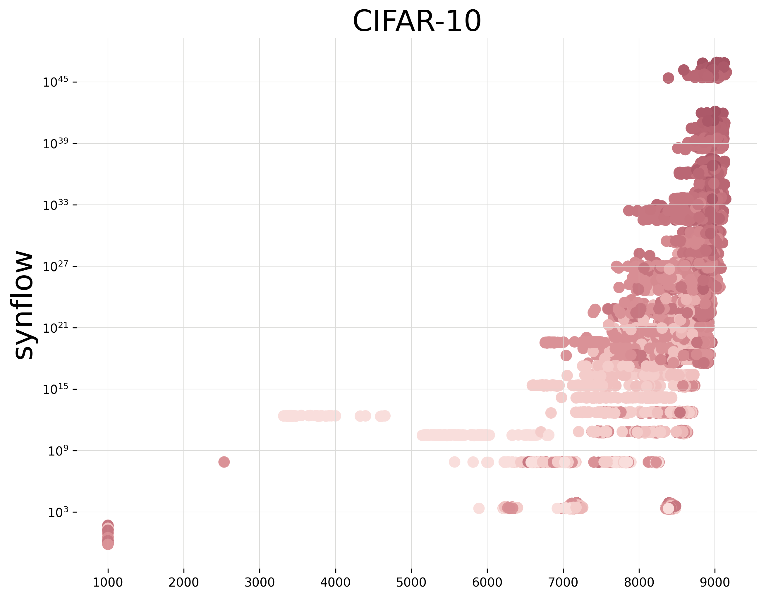
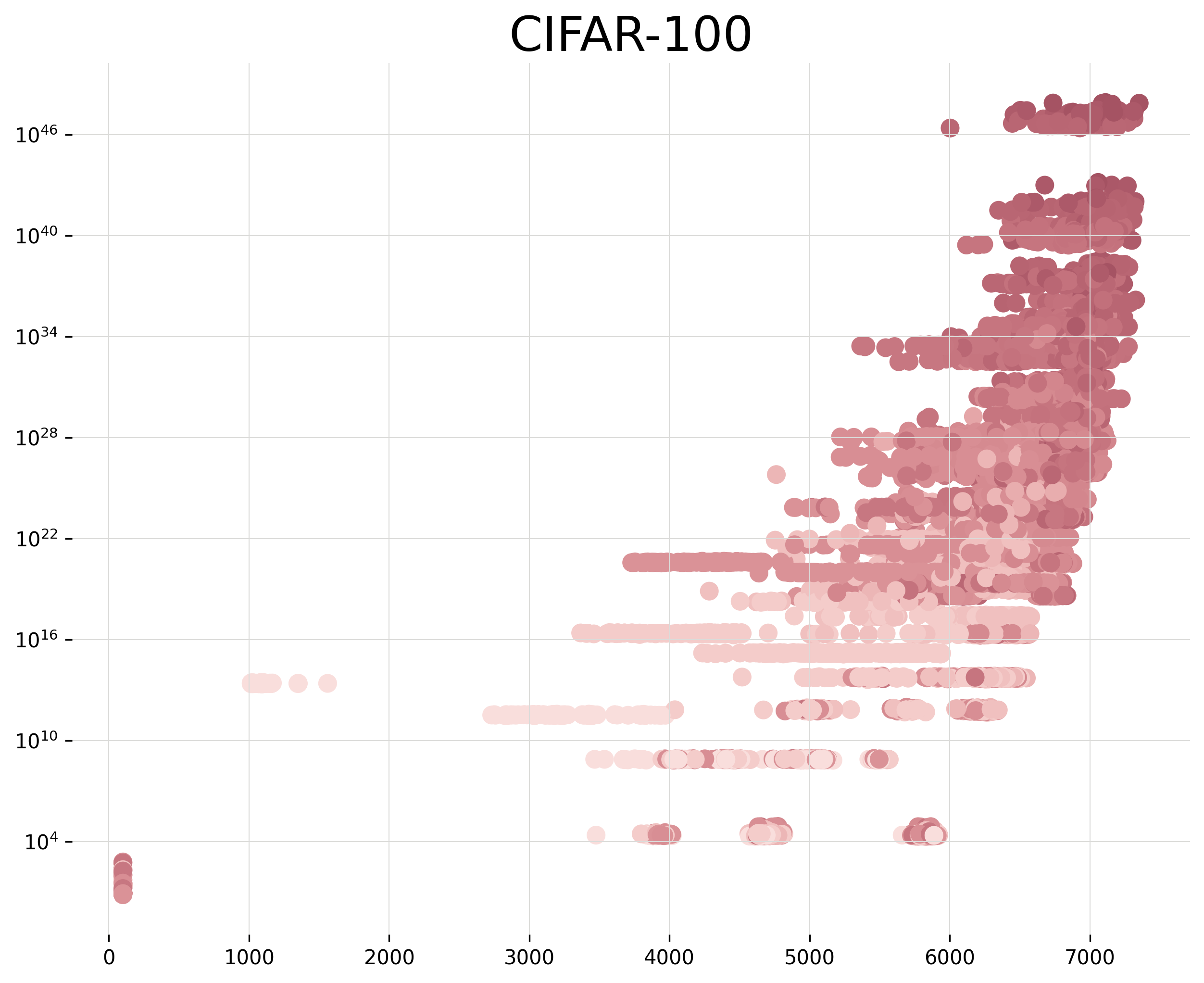
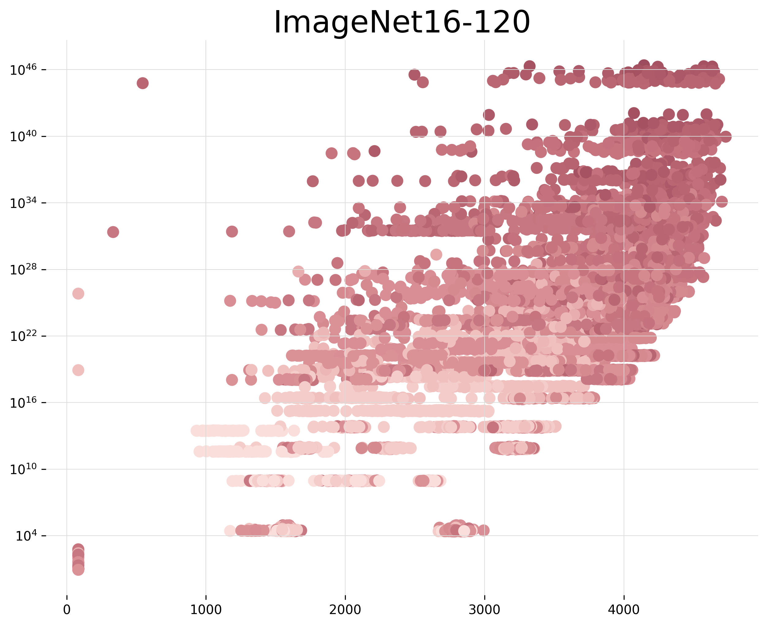
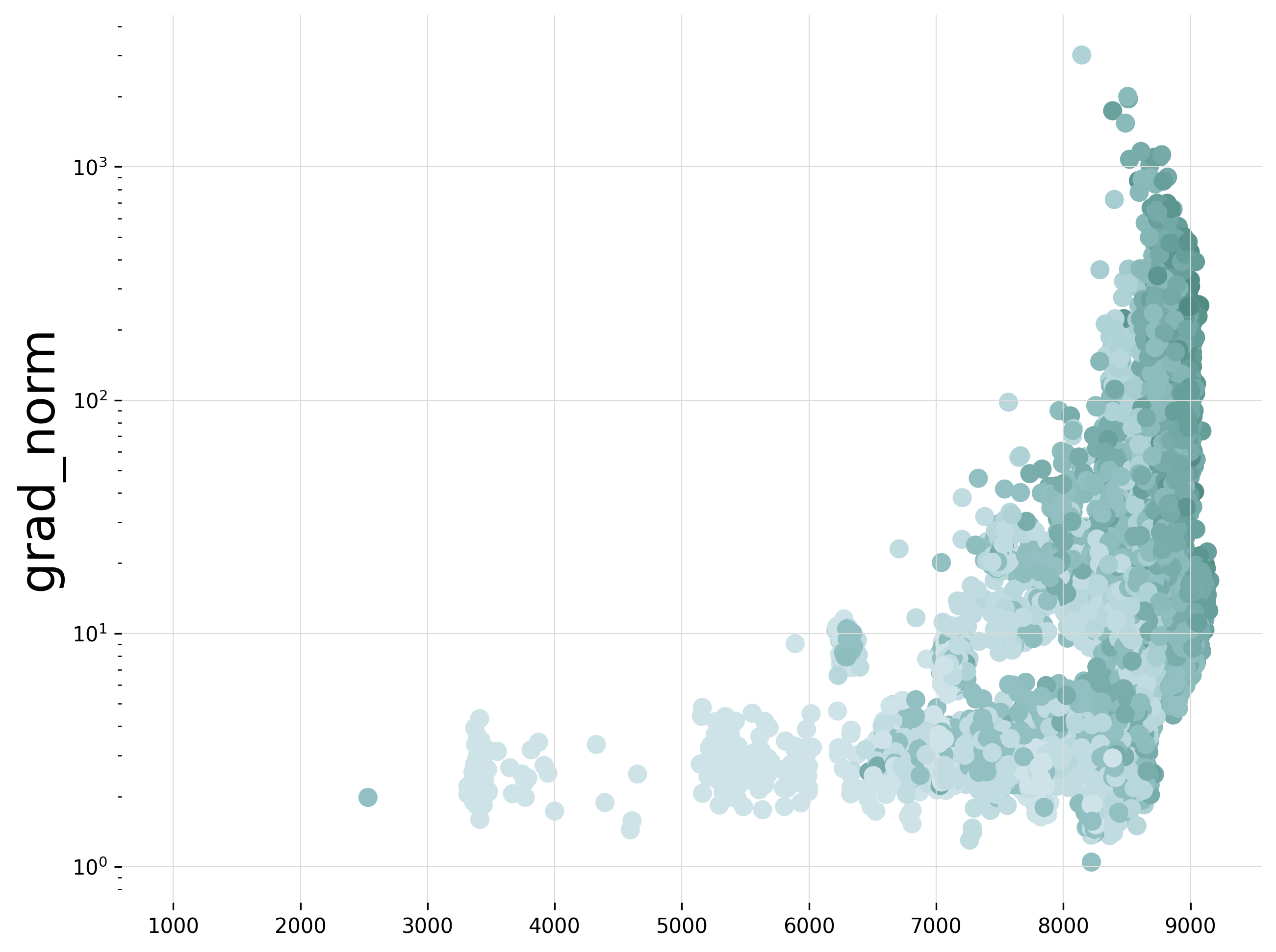
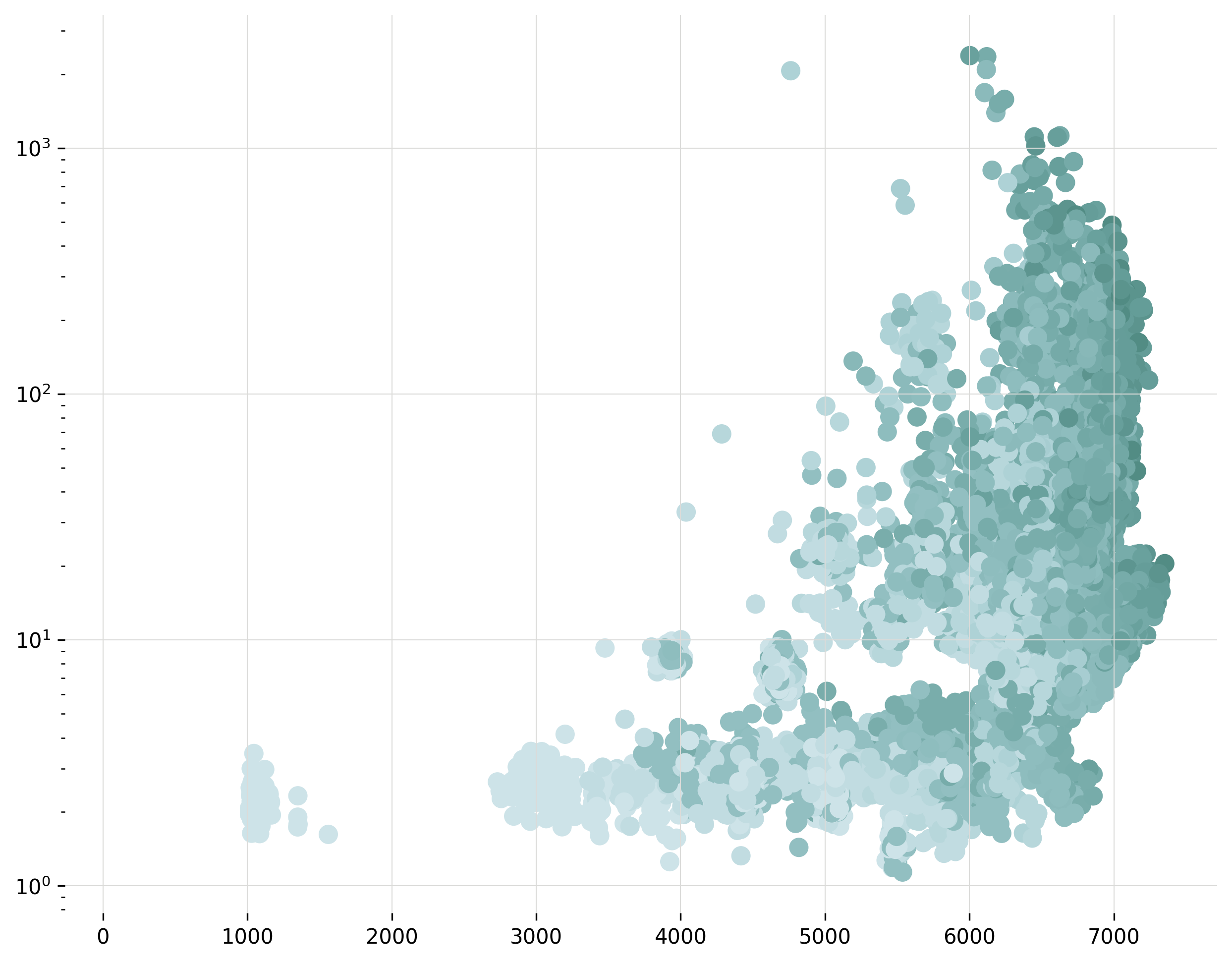
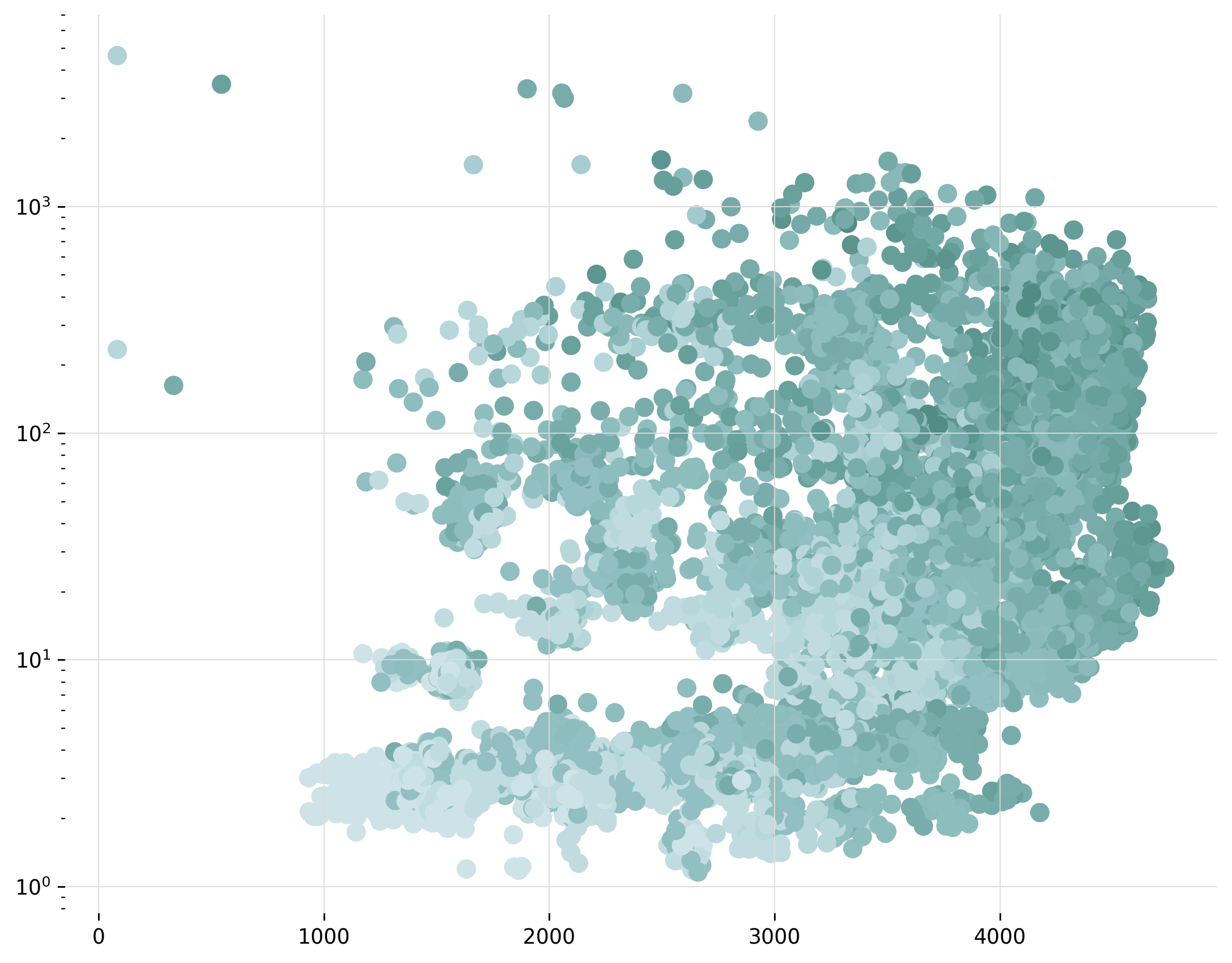
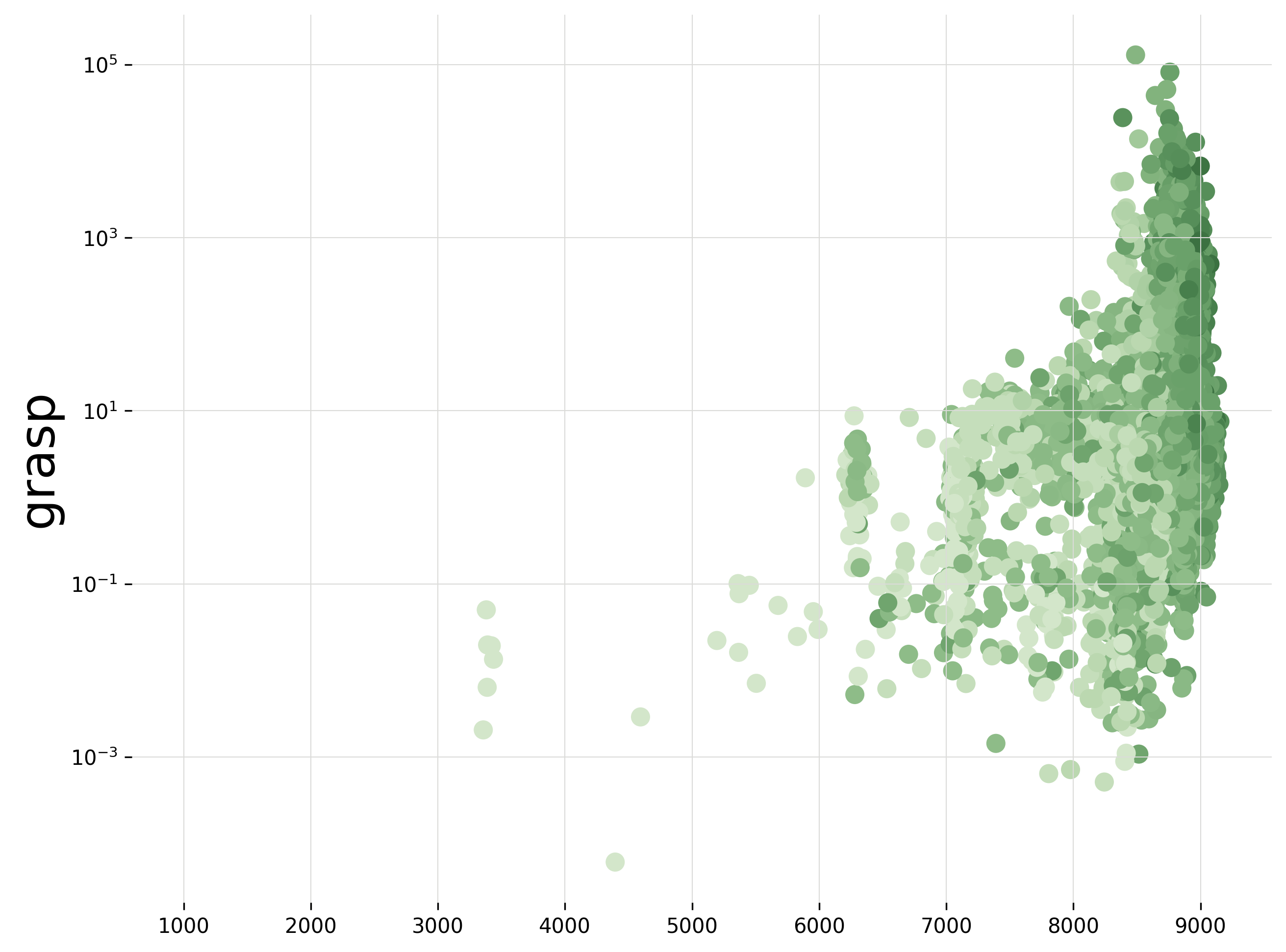
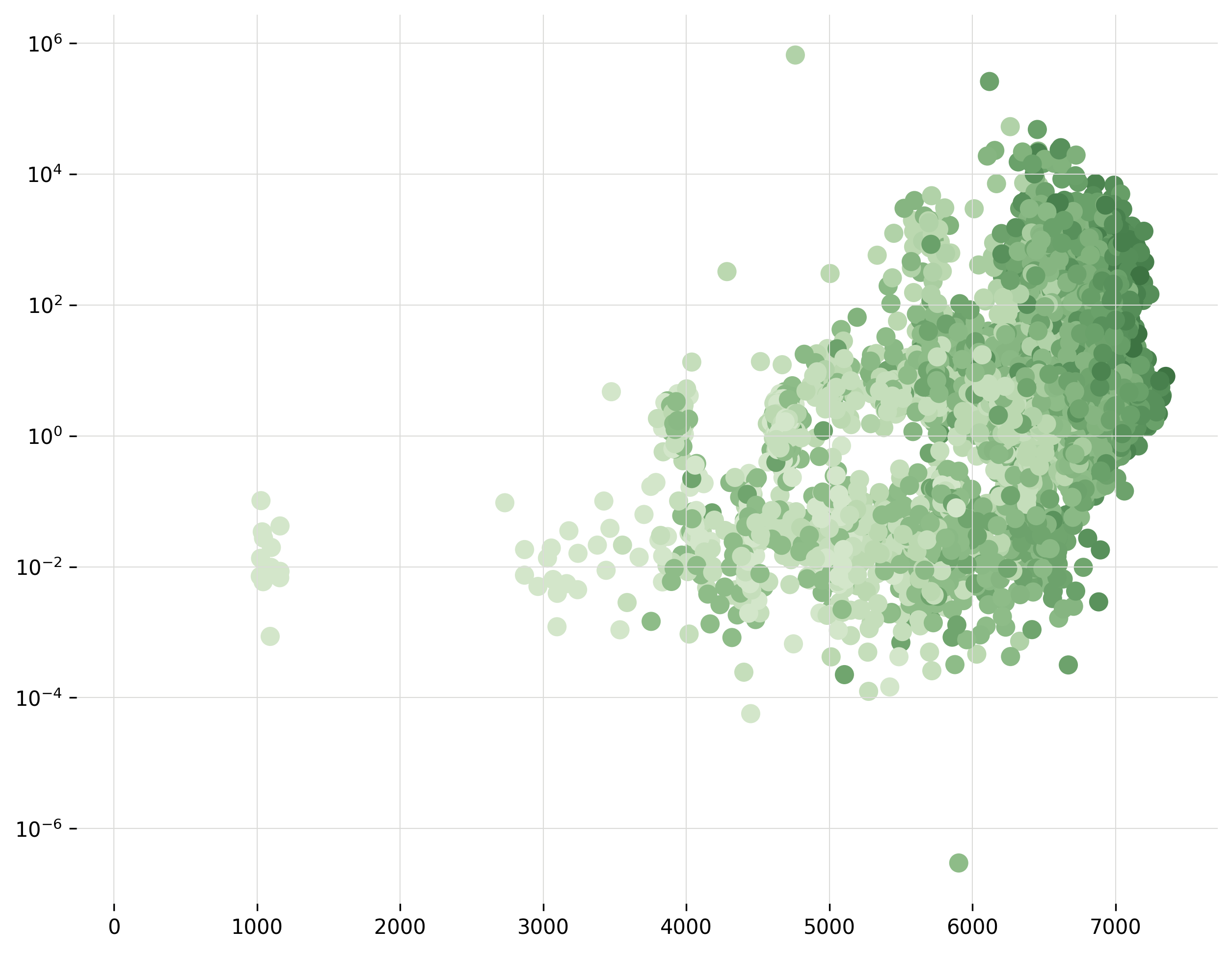
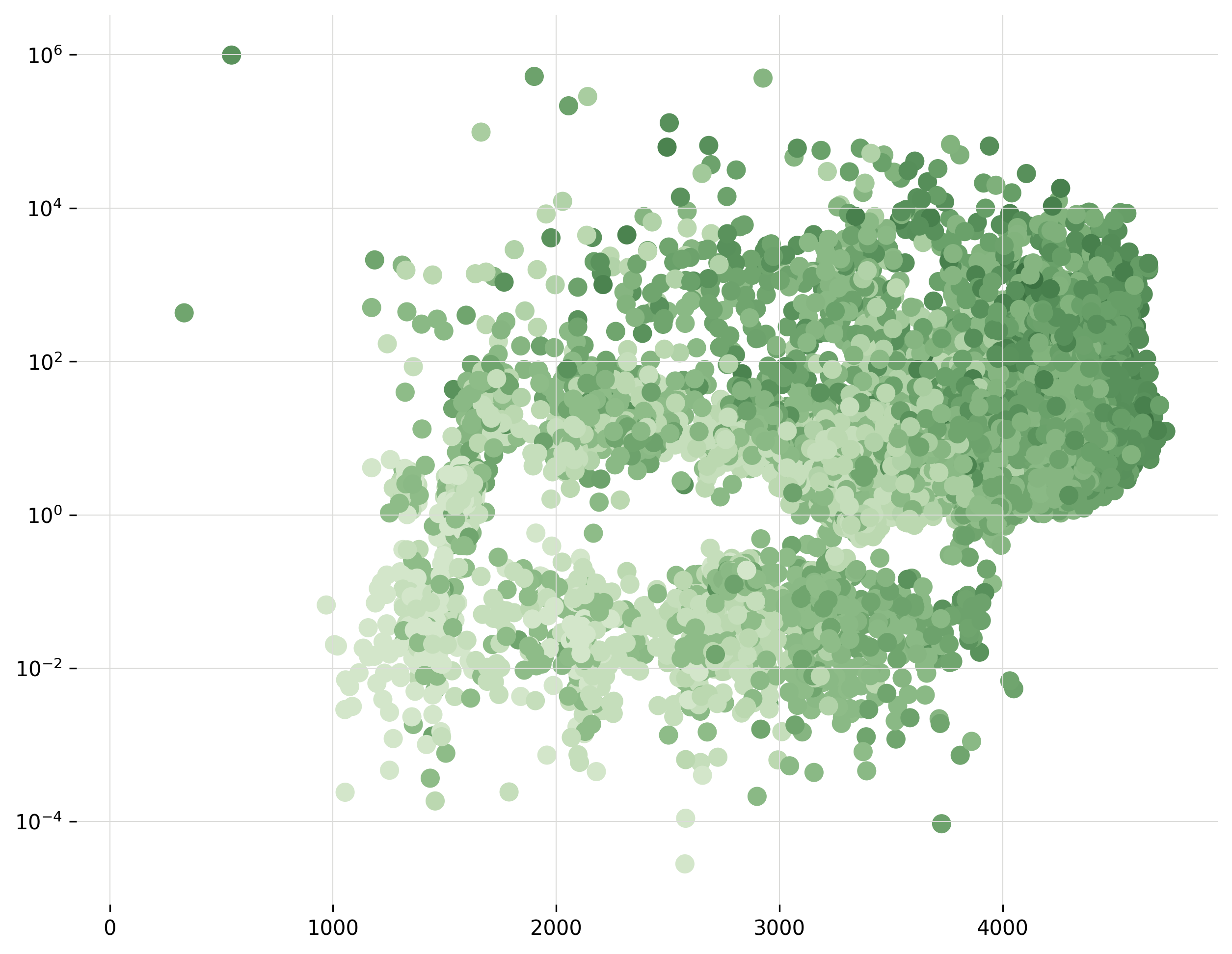
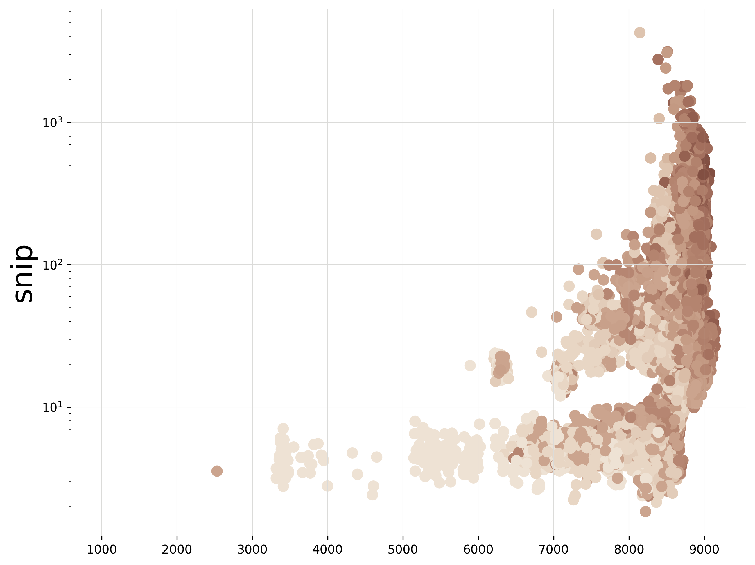
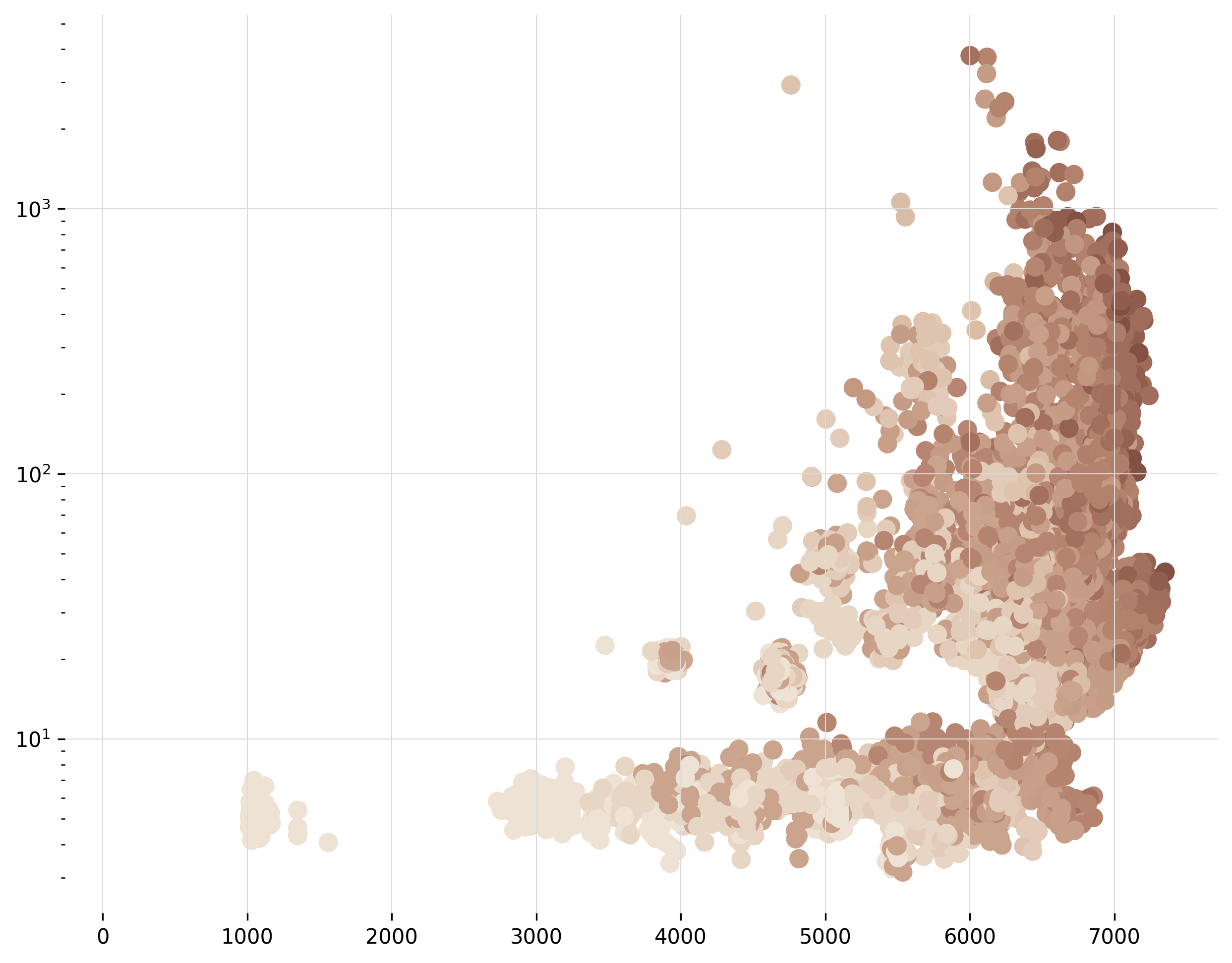
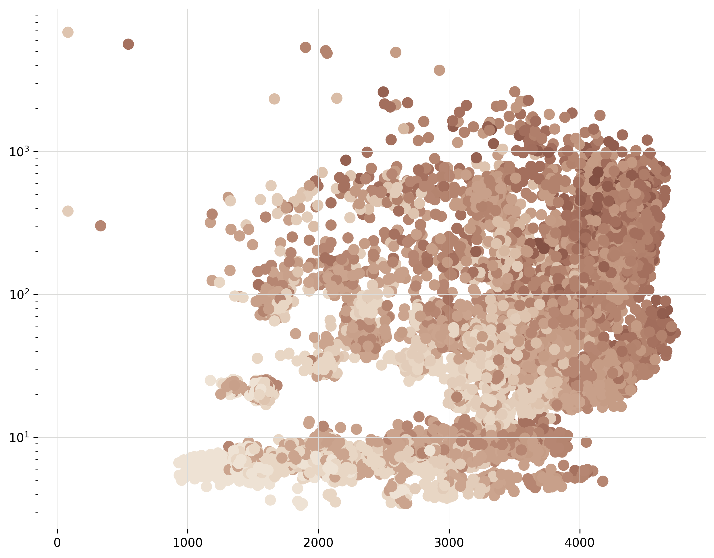
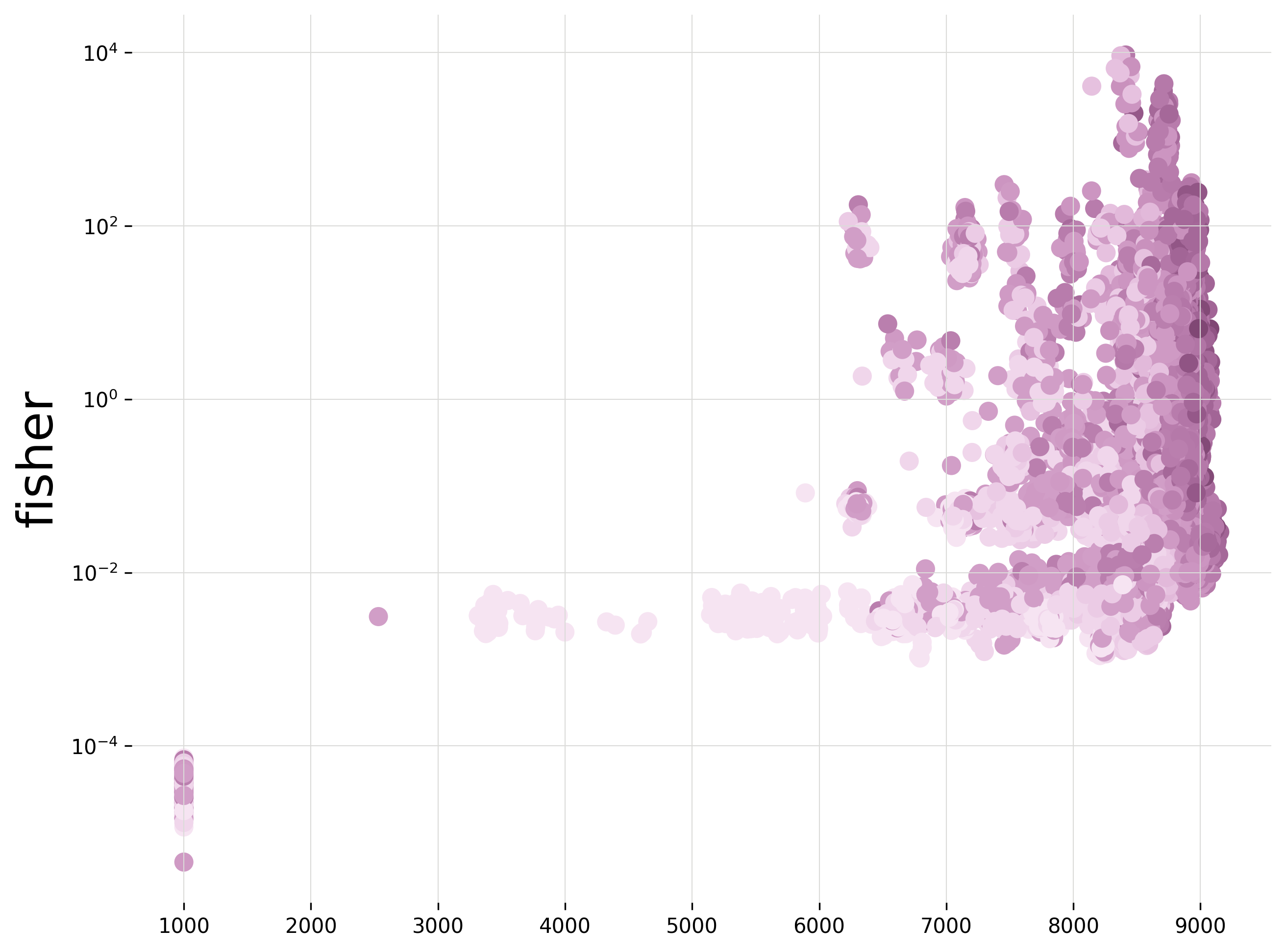
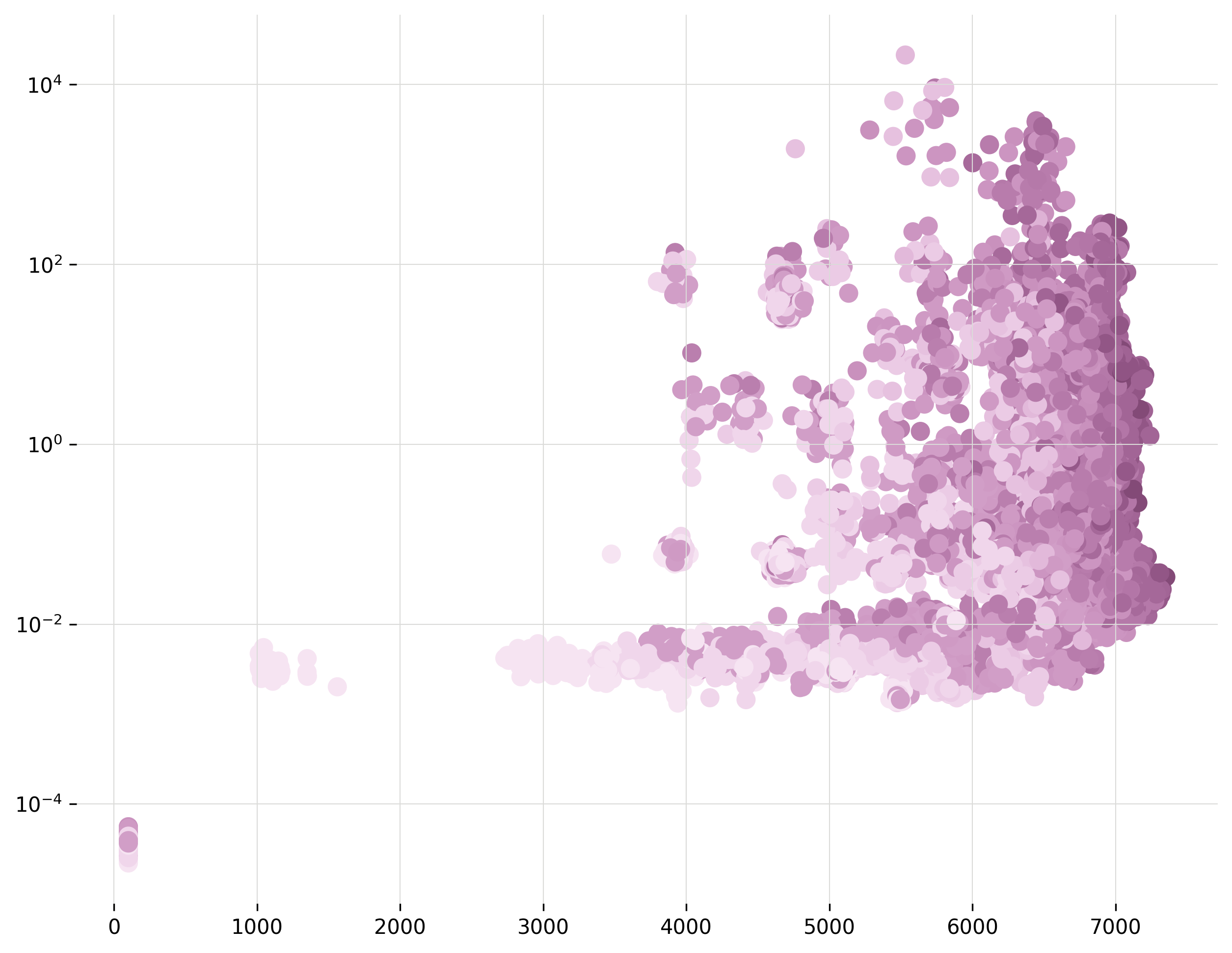
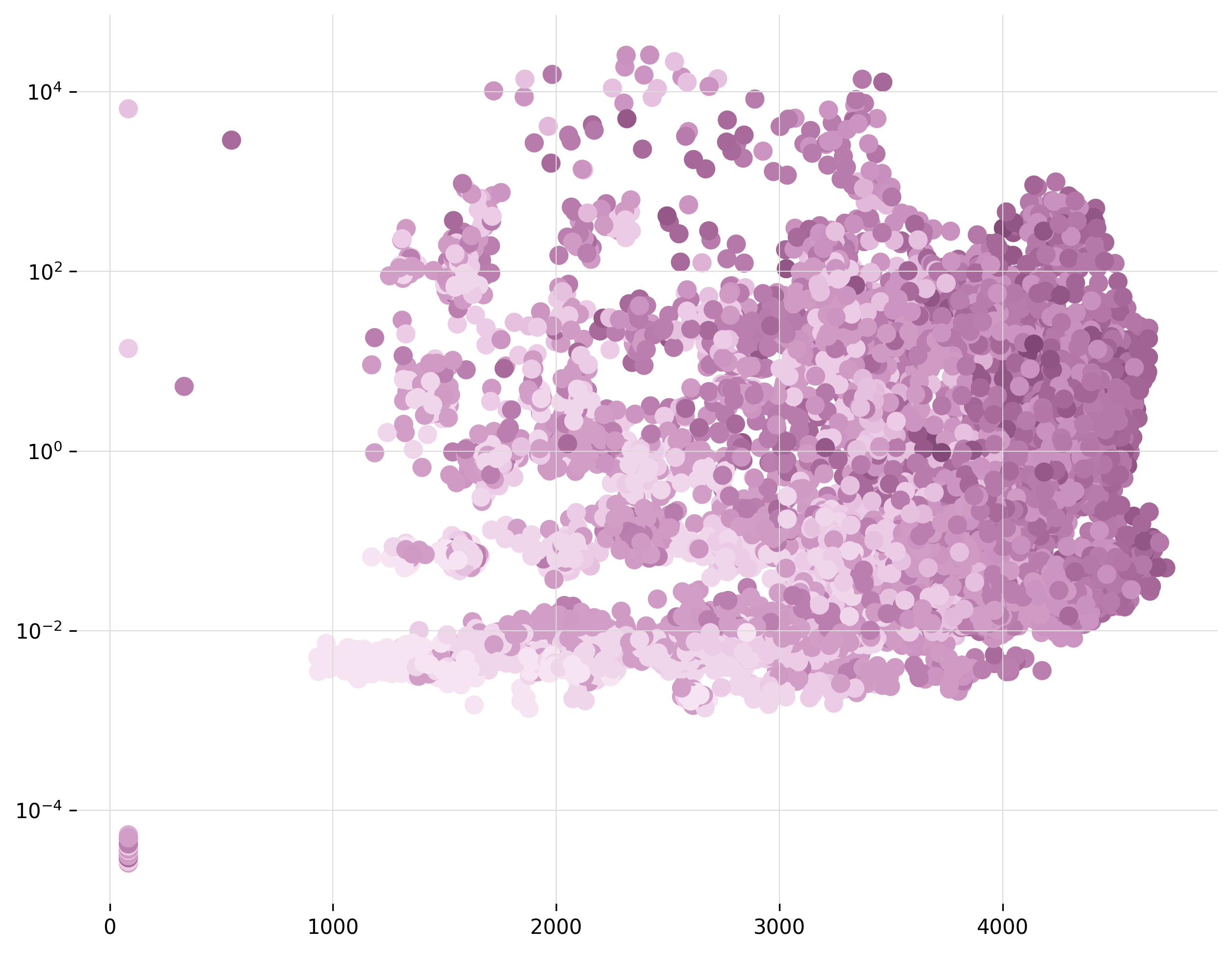
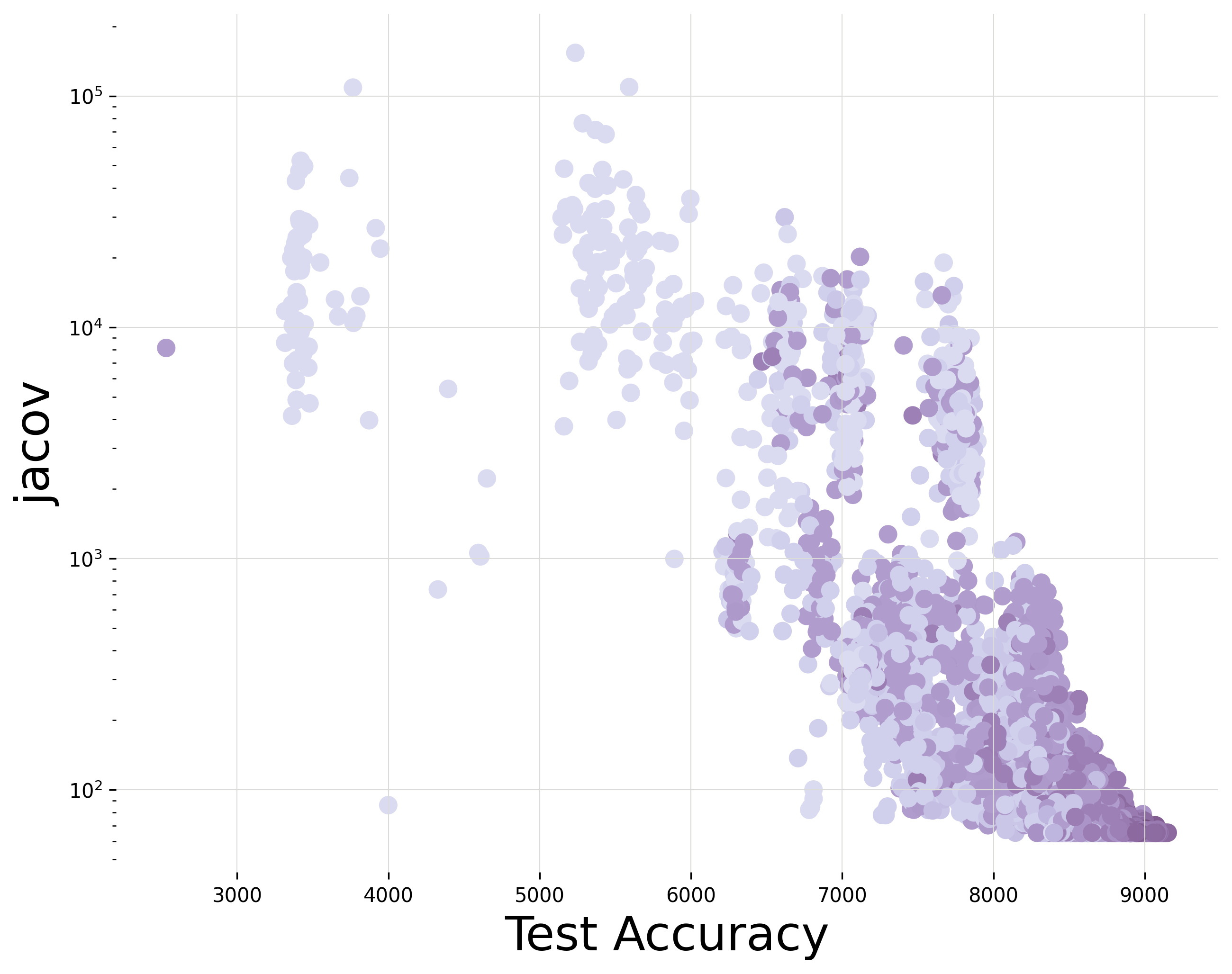
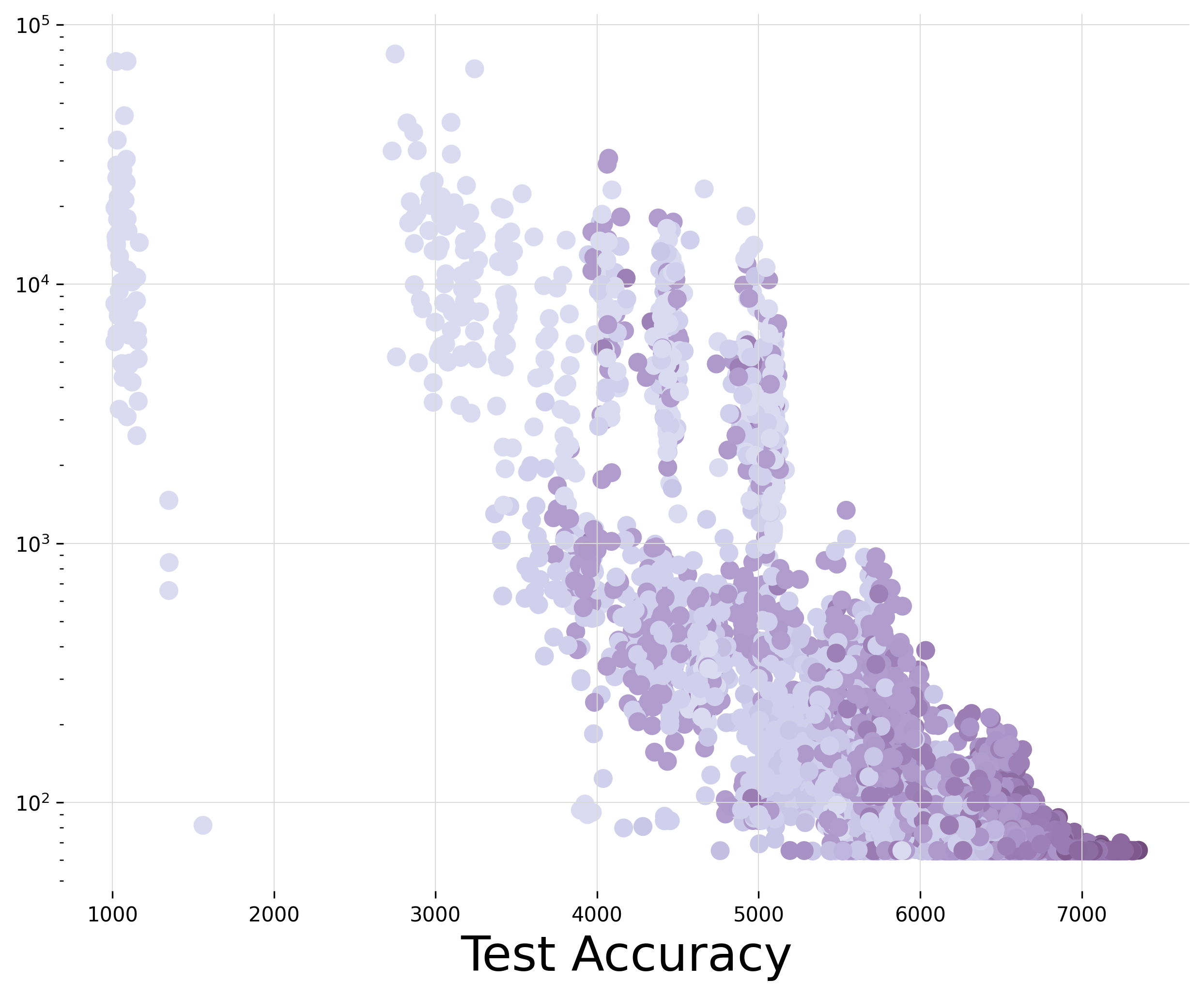
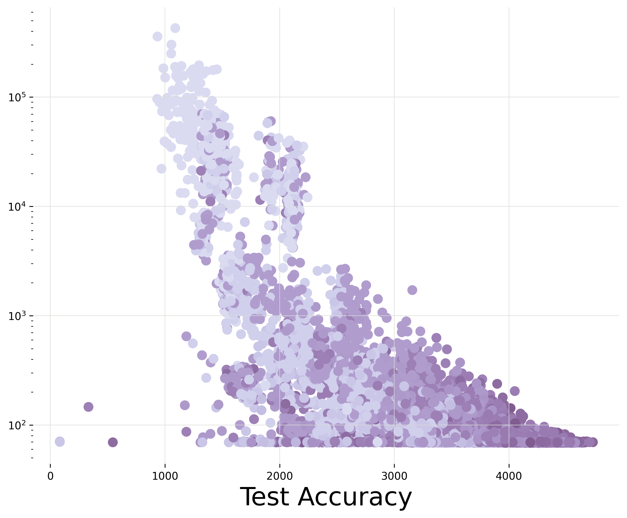
Figure 6: Zero-cost metrics performance illustration for NAS-Bench-201 search space evaluated on CIFAR-10, CIFAR-100 and ImageNet16-120 datasets, based on data from Abdelfattah et al. [2021]. Each dot corresponds to an architecture; the darker the colour, the more parameters it contains. Figure represents search space of $15{,}625$ networks (excluding architectures with NaN scores).

The results for overall epsilon performance on NAS-Bench-201 are given in Table 1 along with other zero-cost NAS metrics. The Kendall $\tau$ score is not reported in Abdelfattah et al. (2021), but it is considered more robust than Spearman $\rho$ and is increasingly used for NAS metric evaluation. We use the data provided by Abdelfattah et al. (2021) to evaluate their Kendal $\tau$. Note that our results differ from the original paper for some evaluation scores. In such cases, we indicate the original values between brackets. In particular, there is a discrepancy in computing the values in the last column, Top-64/top-$5\%$, while the rest of the results are consistent. Figure 6 in Appendix suggests that our calculations are correct.

Table 1: Zero-cost metrics performance for the NAS-Bench-201 search space with its three datasets: CIFAR-10, CIFAR-100 and ImageNet16-120. We give the original values from Abdelfattah et al. (2021) for reference between brackets. We highlight the best-performing metrics in bold.

Metric	Spearman $\rho$					Kendall $\tau$		Top-10%/		Top-64/
	global		top-10%			global	top-10%	top-10%		top-5%
CIFAR-10
grad_sign	0.77
synflow	0.74		0.18			0.54	0.12	45.75	(46)	29	(44)
grad_norm	0.59	(0.58)	-0.36	(-0.38)		0.43	-0.21	30.26	(30)	1	(0)
grasp	0.51	(0.48)	-0.35	(-0.37)		0.36	-0.21	30.77	(30)	3	(0)
snip	0.60	(0.58)	-0.36	(-0.38)		0.44	-0.21	30.65	(31)	1	(0)
fisher	0.36		-0.38			0.26	-0.24	4.99	( 5)	0	(0)
jacov	-0.73	(0.73)	0.15	(0.17)		0.55	-0.10	24.72	(25)	11	(15)
epsilon	0.87		0.55			0.70	0.40	67.39		59
CIFAR-100
grad_sign	0.79
synflow	0.76		0.42			0.57	0.29	49.71	(50)	45	(54)
grad_norm	0.64		-0.09			0.47	-0.05	35.00	(35)	0	(4)
grasp	0.55	(0.54)	-0.10	(-0.11)		0.39	-0.06	35.32	(34)	3	(4)
snip	0.64	(0.63)	-0.08	(-0.09)		0.47	-0.05	35.25	(36)	0	(4)
fisher	0.39		-0.15	(-0.16)		0.28	-0.10	4.22	( 4)	0	(0)
jacov	-0.70	(0.71)	0.07	(0.08)		0.54	0.05	22.11	(24)	7	(15)
epsilon	0.90		0.59			0.72	0.43	81.24		62
ImageNet16-120
grad_sign	0.78
synflow	0.75		0.55			0.56	0.39	43.57	(44)	26	(56)
grad_norm	0.58		0.12	(0.13)		0.43	0.09	31.29	(31)	0	(13)
grasp	0.55	(0.56)	0.10			0.39	0.07	31.61	(32)	2	(14)
snip	0.58		0.13			0.43	0.09	31.16	(31)	0	(13)
fisher	0.33		0.02			0.25	0.01	4.61	( 5)	0	(0)
jacov	0.70	(0.71)	0.08	(0.05)		0.53	0.05	29.63	(44)	10	(15)
epsilon	0.85		0.53			0.67	0.37	71.51		59

For NAS-Bench-201, we also report average performance when selecting one architecture from a pool of $N$ random architectures. The statistics are reported over $500$ runs. Table 2 compares epsilon to other trainless metrics. Note that te-nas starts with a super-network composed of all the edges and operators available within the space. In this case, $N$ is not applicable, and the performance can not be improved. In principle, other methods’ performance should improve with higher $N$ values.

Table 2: Comparison of the trainless metrics performances against existing NAS algorithms on CIFAR-10, CIFAR-100 and ImageNet16-120 datasets. On the top, we list the best-performing methods that require training (REA Real et al. (2019), random search, REINFORCE Williams (1992), BOHB Falkner et al. (2018)). We report the average best-achieved test accuracy over $500$ runs, with $1{,}000$ architectures ($100$ for grad_sign)sampled from the search space at random. For tenas, the results are reported for $4$ random seeds. Random and optimal performances are given as baseline.

Method	CIFAR-10			CIFAR-100			ImageNet16-120
	validation	test		validation	test		validation	test
State-of-the-art
REA	$91.19\pm 0.31$	$93.92\pm 0.3$		$71.81\pm 1.12$	$71.84\pm 0.99$		$45.15\pm 0.89$	$45.54\pm 1.03$
Random Search	$90.93\pm 0.36$	$93.92\pm 0.31$		$70.93\pm 1.09$	$71.04\pm 1.07$		$44.45\pm 1.1$	$44.57\pm 1.25$
REINFORCE	$91.09\pm 0.37$	$93.92\pm 0.32$		$71.61\pm 1.12$	$71.71\pm 1.09$		$45.05\pm 1.02$	$45.24\pm 1.18$
BOHB	$90.82\pm 0.53$	$93.92\pm 0.33$		$70.74\pm 1.29$	$70.85\pm 1.28$		$44.26\pm 1.36$	$44.42\pm 1.49$
Baselines (N=1000)
Optimal	$91.34\pm 0.18$	$94.20\pm 0.13$		$72.53\pm 0.53$	$72.84\pm 0.41$		$45.93\pm 0.51$	$46.59\pm 0.34$
Random	$84.11\pm 11.71$	$87.40\pm 11.94$		$61.57\pm 11.305$	$61.67\pm 11.35$		$33.97\pm 8.68$	$33.67\pm 8.98$
Trainless (N=1000)
naswot	$89.69\pm 0.73$	$92.96\pm 0.81$		$69.86\pm 1.21$	$69.98\pm 1.22$		$43.95\pm 2.05$	$44.44\pm 2.10$
synflow	$89.91\pm 0.83$	$90.12\pm 0.78$		$70.35\pm 2.25$	$70.37\pm 2.08$		$41.73\pm 3.91$	$42.11\pm 4.02$
grad_norm	$88.13\pm 2.35$	$88.42\pm 2.28$		$66.35\pm 5.45$	$66.48\pm 5.32$		$33.88\pm 11.46$	$33.90\pm 11.74$
grasp	$87.85\pm 2.12$	$88.17\pm 2.04$		$65.36\pm 5.57$	$65.45\pm 5.48$		$32.23\pm 10.95$	$32.20\pm 11.23$
snip	$87.47\pm 2.19$	$87.81\pm 2.12$		$64.61\pm 5.52$	$64.74\pm 5.43$		$30.65\pm 11.32$	$30.55\pm 11.55$
fisher	$87.01\pm 2.31$	$87.36\pm 2.23$		$63.54\pm 5.69$	$63.67\pm 5.62$		$26.70\pm 10.83$	$29.56\pm 10.83$
jacov	$88.17\pm 1.67$	$88.45\pm 1.69$		$67.73\pm 2.69$	$67.90\pm 2.77$		$31.58\pm 10.65$	$31.44\pm 10.83$
epsilon	$\boldsymbol{91.03}\pm\boldsymbol{0.42}$	$\boldsymbol{93.86}\pm\boldsymbol{0.43}$		$\boldsymbol{71.76}\pm\boldsymbol{0.90}$	$\boldsymbol{71.79}\pm\boldsymbol{0.86}$		$\boldsymbol{45.11}\pm\boldsymbol{0.99}$	$\boldsymbol{45.42}\pm\boldsymbol{1.21}$
Trainless (N=100)
grad_sign	$89.84\pm 0.61$	$93.31\pm 0.47$		$70.22\pm 1.32$	$70.33\pm 1.28$		$42.07\pm 2.78$	$42.42\pm 2.81$
epsilon	$\boldsymbol{90.44}\pm\boldsymbol{0.97}$	$\boldsymbol{93.39}\pm\boldsymbol{0.82}$		$\boldsymbol{70.85}\pm\boldsymbol{1.30}$	$\boldsymbol{71.00}\pm\boldsymbol{1.26}$		$\boldsymbol{44.03}\pm\boldsymbol{2.02}$	$\boldsymbol{44.20}\pm\boldsymbol{2.04}$
Trainless (N/A)
tenas		$93.9\pm 0.47$			$71.24\pm 0.56$			$42.38\pm 0.46$

Comparing the results for epsilon with other zero-cost NAS metrics, we can see that it outperforms them by a good margin. Figure 1 further confirms the applicability of the method to the NAS-Bench-201 field (similar figures for other methods can be found in Appendix, Figure 6). However, NAS-Bench-201 is a relatively compact search space; furthermore, it has been used for epsilon development.

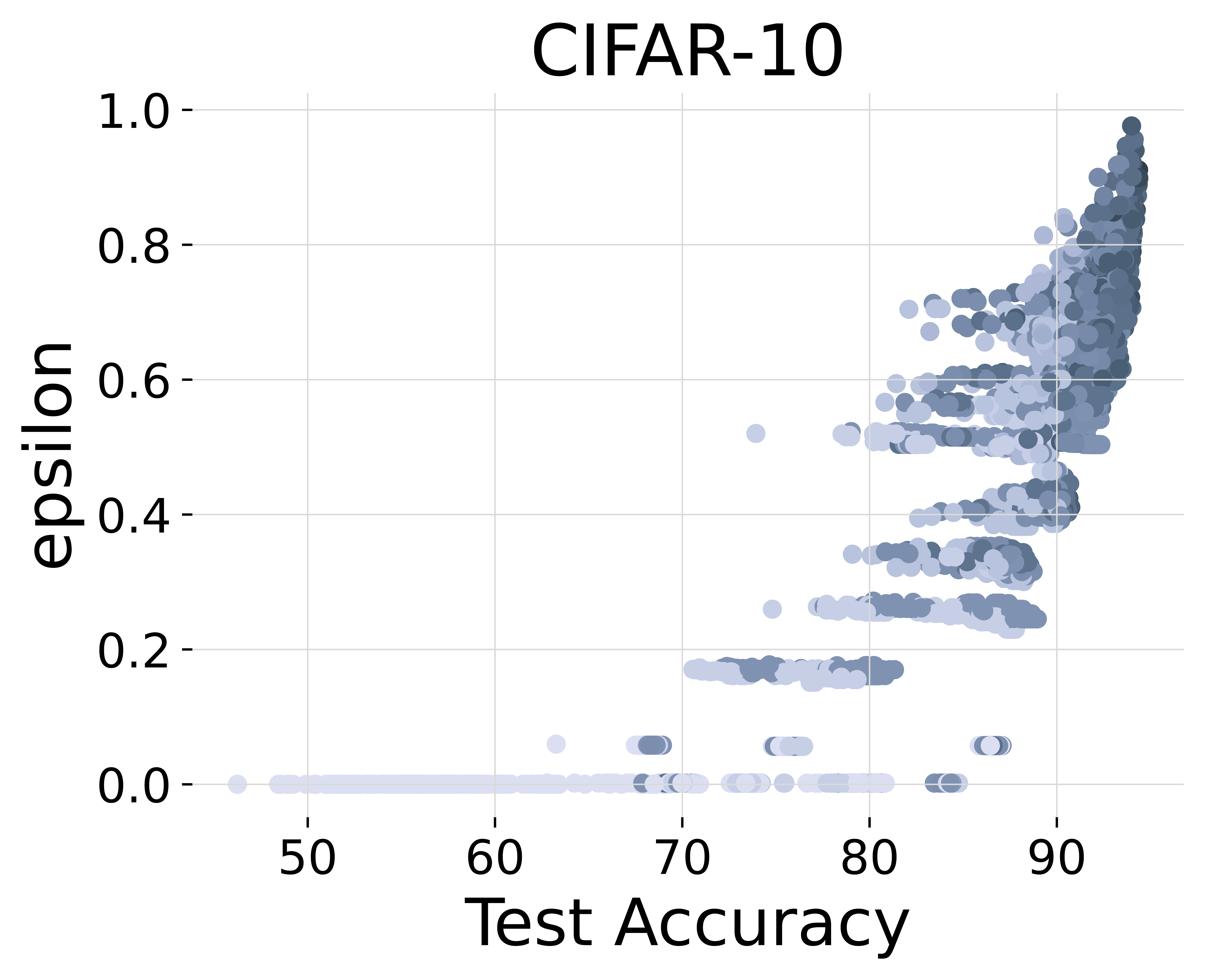
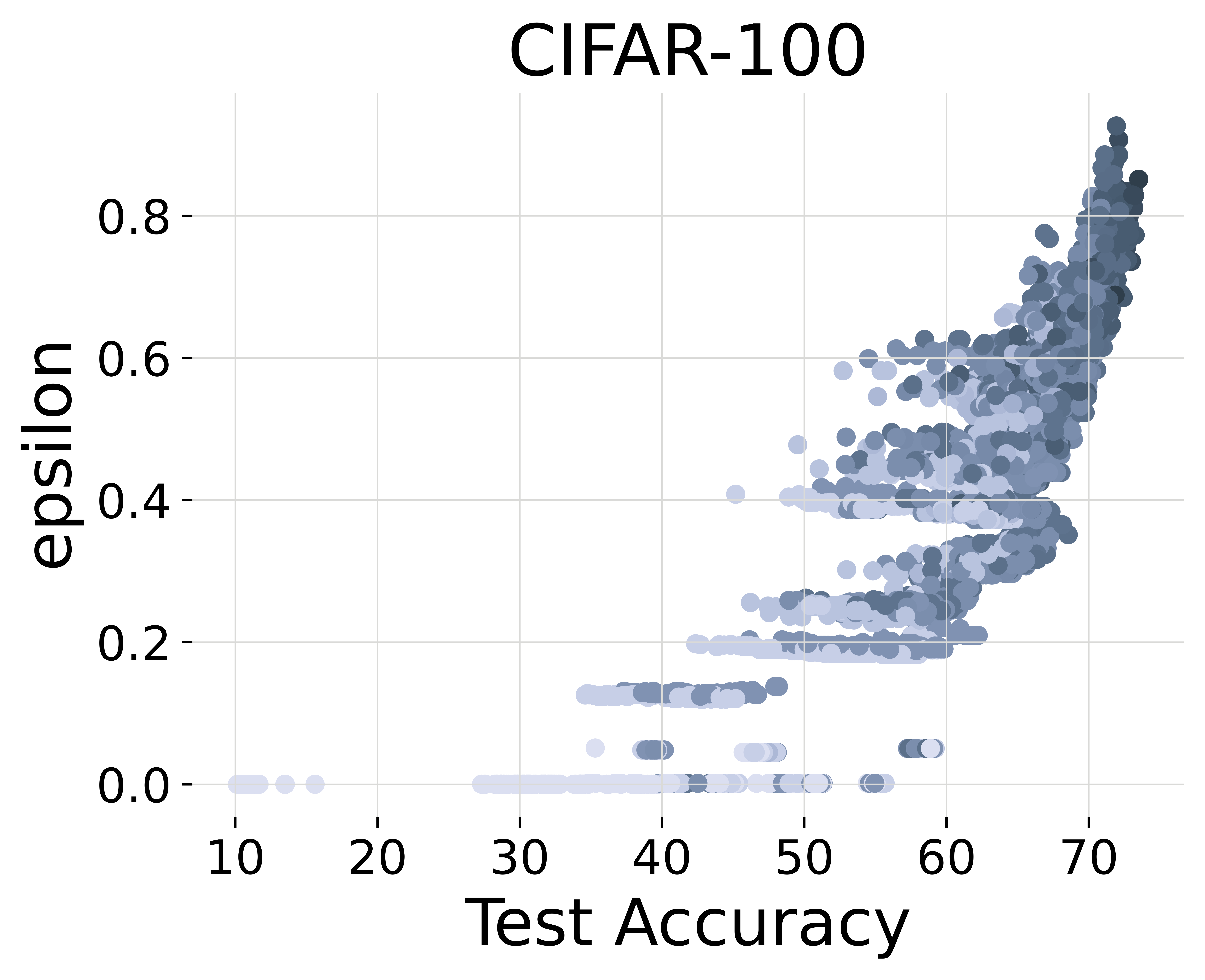
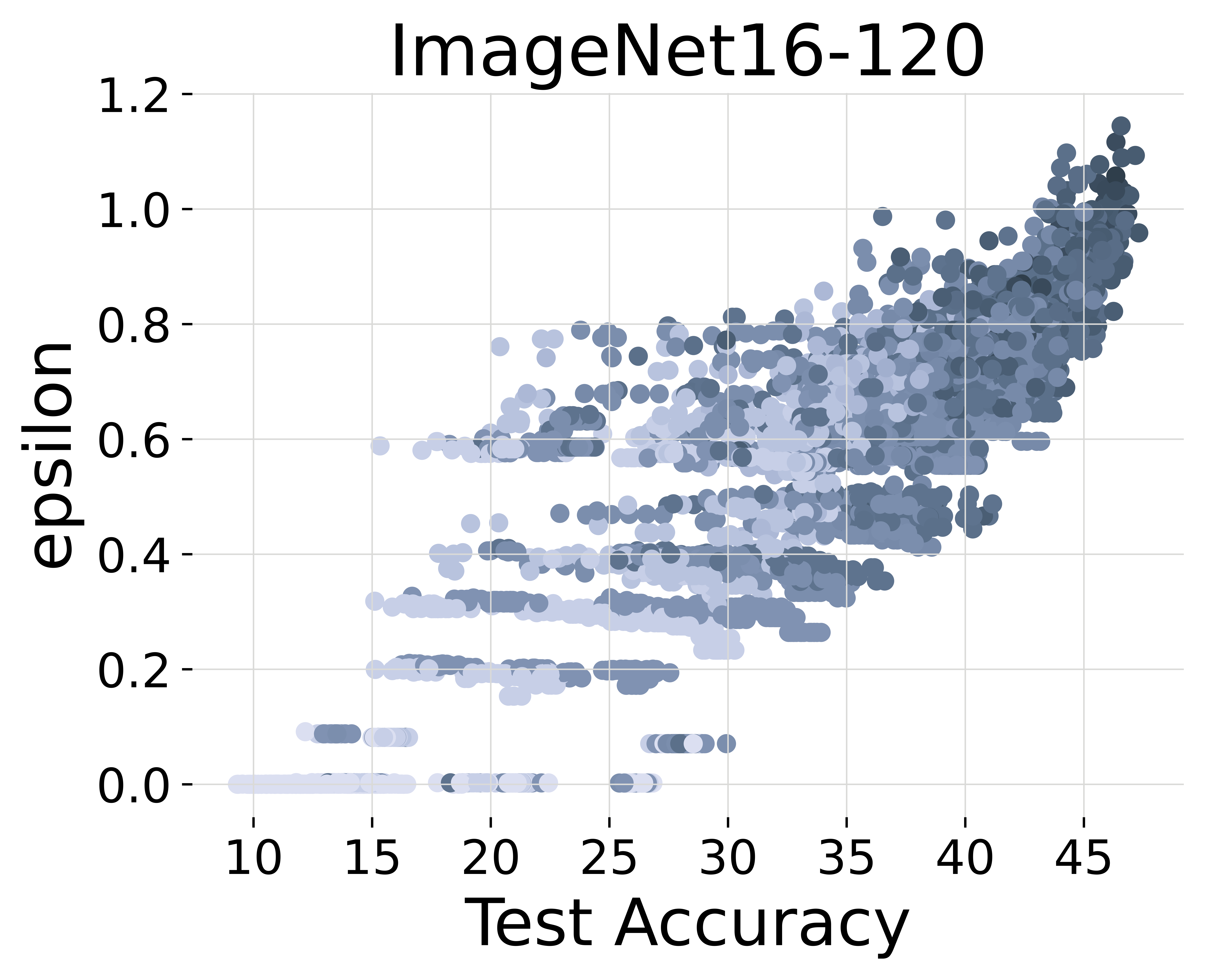
Figure 1: Zero-cost NAS epsilon metric performance illustration for NAS-Bench-201 search space evaluated on CIFAR-10, CIFAR-100 and ImageNet16-120 datasets. The horizontal axis shows test accuracy upon training. Each dot corresponds to an architecture; the darker the colour, the more parameters it contains. The figure represents the search space of $15{,}625$ networks (excluding architectures with NaN scores).

3.1.2 NAS-Bench-101

We use NAS-Bench-101 space to confirm that the success of epsilon metric in the previous section is not due to overfitting the NAS-Bench-201 search space and to see how it applies to a vaster search space. Table 3 together with Figure 2 confirm that it performs reasonably well on NAS-Bench-101, too.

Table 3: Zero-cost metrics performance evaluated on NAS-Bench-101 search space, CIFAR-10 dataset. Values from Abdelfattah et al. (2021) are given for reference between brackets. We highlight the best-performing metrics in bold.

Metric	Spearman $\rho$					Kendall $\tau$		Top-10%/		Top-64/
	global		top-10%			global	top-10%	top-10%		top-5%
CIFAR-10
grad_sign	0.45
synflow	0.37		0.14			0.25	0.10	22.67	23	4	(12)
grad_norm	-0.20		-0.05	(0.05)		-0.14	-0.03	1.98	2	0	(0)
grasp	0.45		-0.01			0.31	-0.01	25.60	26	0	(6)
snip	-0.16		0.01	(-0.01)		-0.11	0.00	3.43	3	0	(0)
fisher	-0.26		-0.07	(0.07)		-0.18	-0.05	2.65	3	0	(0)
jacov	0.38	(0.38)	-0.08	(0.08)		-0.05	0.05	1.66	2	0	(0)
epsilon	0.62		0.12			0.44	0.08	40.33		10

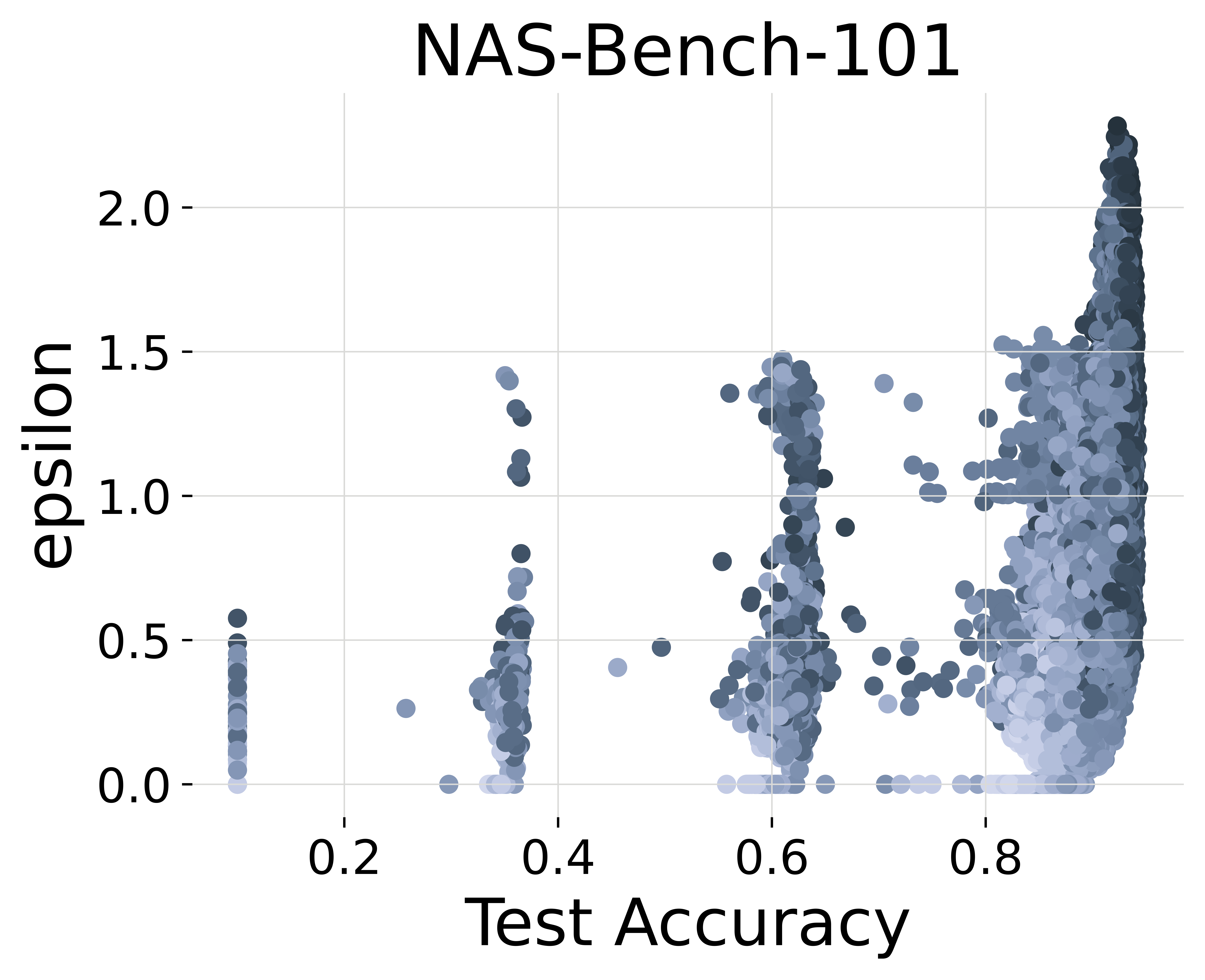
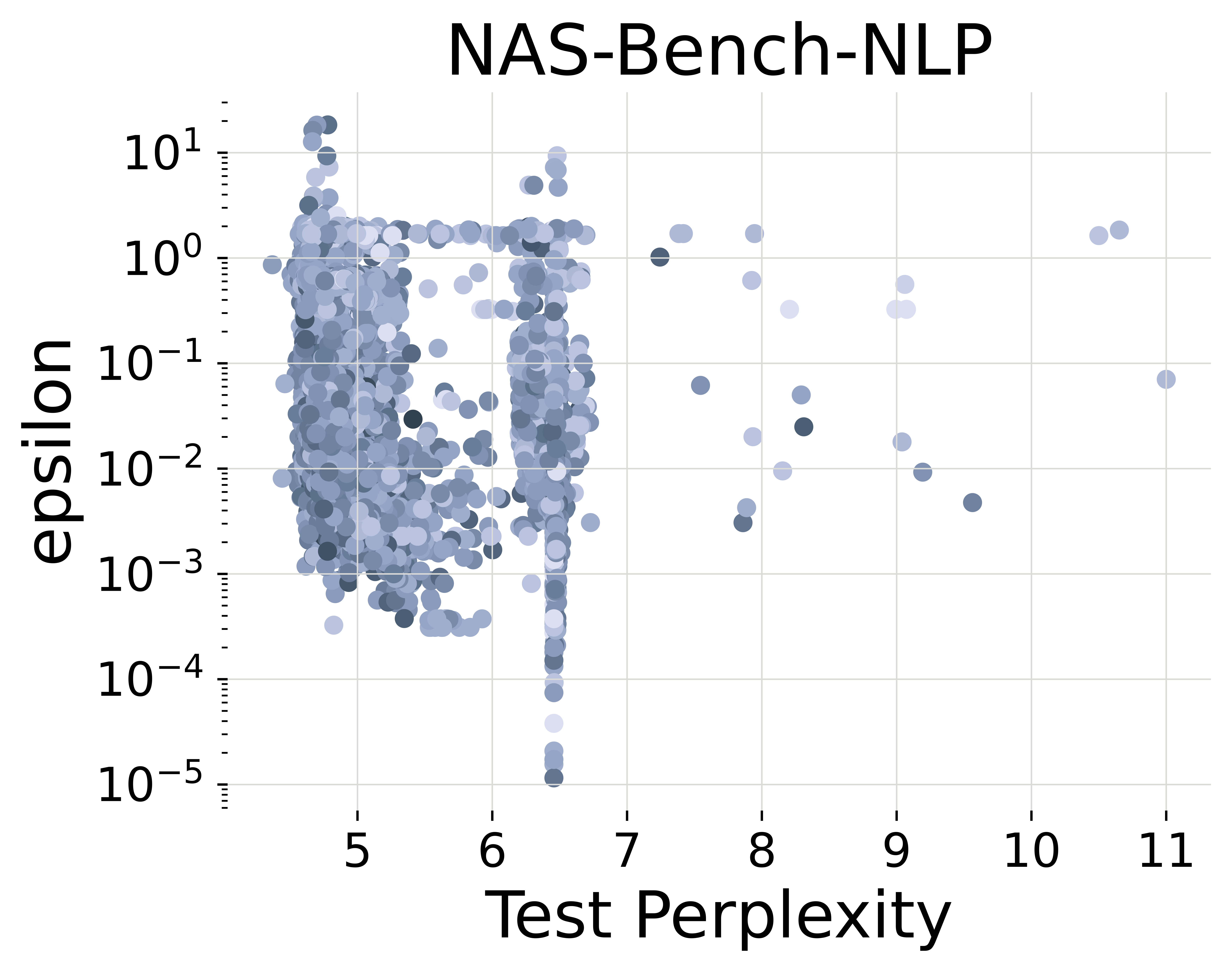
Figure 2: Zero-cost NAS epsilon metric performance illustration for NAS-Bench-101 search space, CIFAR-10 dataset and NAS-Bench-NLP search space, PTB dataset. The horizontal axis shows test accuracy upon training. Each dot corresponds to an architecture; the darker the colour, the more parameters it contains. The figure shows $423{,}624$ and $14{,}322$ networks for NAS-Bench-101 and NAS-Bench-NLP, respectively (excluding architectures with NaN scores).

3.1.3 NAS-Bench-NLP

Both NAS-Bench-201 and NAS-Bench-101 are created to facilitate NAS in image recognition. They operate convolutional networks of very similar constitutions. To truly probe the generalisability of the epsilon metric, we test it on NAS-Bench-NLP. Both input data format and architecture type differ from the first two search spaces.

Unfortunately, Abdelfattah et al. (2021) provides no data for NAS-Bench-NLP, disabling us from using their results for calculations. Therefore, in Table 4, we give only values provided in the paper together with our epsilon metric (data for ficher is absent). We want to note that, unlike accuracy, perplexity used for language-related ML problems should be minimised. Therefore, the signs of correlations with scoring metrics should be reversed, which is not the case for numbers given in Abdelfattah et al. (2021).

The performance of epsilon metric on the NAS-Bench-NLP space is not exceptional. While there is a trend towards better architectures with increasing metric value, the noise level is beyond acceptable. It might stem from the characteristics of the benchmark itself (factors like a relatively small sample of networks given vast space, chosen hyperparameters, dropout rates, and others may distort NAS performance). Nonetheless, the trend is visible enough to conclude that epsilon metric can apply to recurrent type architectures.

Table 4: Zero-cost metrics performance evaluated on NAS-Bench-NLP search space, PTB dataset. We highlight the best-performing metrics in bold.

Metric	Spearman $\rho$			Kendall $\tau$		Top-10%/	Top-64/
	global	top-10%		global	top-10%	top-10%	top-5%
PTB
synflow	0.34	0.10		—	—	22	—
grad_norm	-0.21	0.03		—	—	10	—
grasp	0.16	0.55		—	—	4	—
snip	-0.19	-0.02		—	—	10	—
jacov	0.38	0.04		—	—	38	—
epsilon	-0.34	-0.12		-0.23	-0.08	24.87	11

3.2 Integration with other NAS methods

While it is possible to utilise zero-cost metrics independently, they are often implemented within other NAS. Here we provide examples of random search and ageing evolution algorithms when used in tandem with epsilon.

Similarly to Abdelfattah et al. (2021), we compare random search performance with and without warm-up. First, we create a warm-up pool of $3{,}000$ architectures. Then, during the first $64$ steps of random search, the algorithm picks networks from the pool based on the highest trainless score and accordingly updates the best test performance.

For ageing evolution, the same principle applies. En plus, we report the results of implementation where every next parent is decided based on the highest epsilon score ("move"). In other words, the trainless scoring metric replaces validation accuracy in move mode. Finally, the child is created by parent mutation (within an edit distance of $1$) and added to the pool. Finally, the oldest network is removed from the pool.

For both described algorithms, we run the procedure until the number of trained architectures reaches $300$ and perform $100$ random rounds. Figure 3 shows that epsilon metric leads to considerable improvements in terms of time and precision. The best performance is achieved in combination with a warm-up. Figure 5 assembles warm-up performances for several trainless metrics.

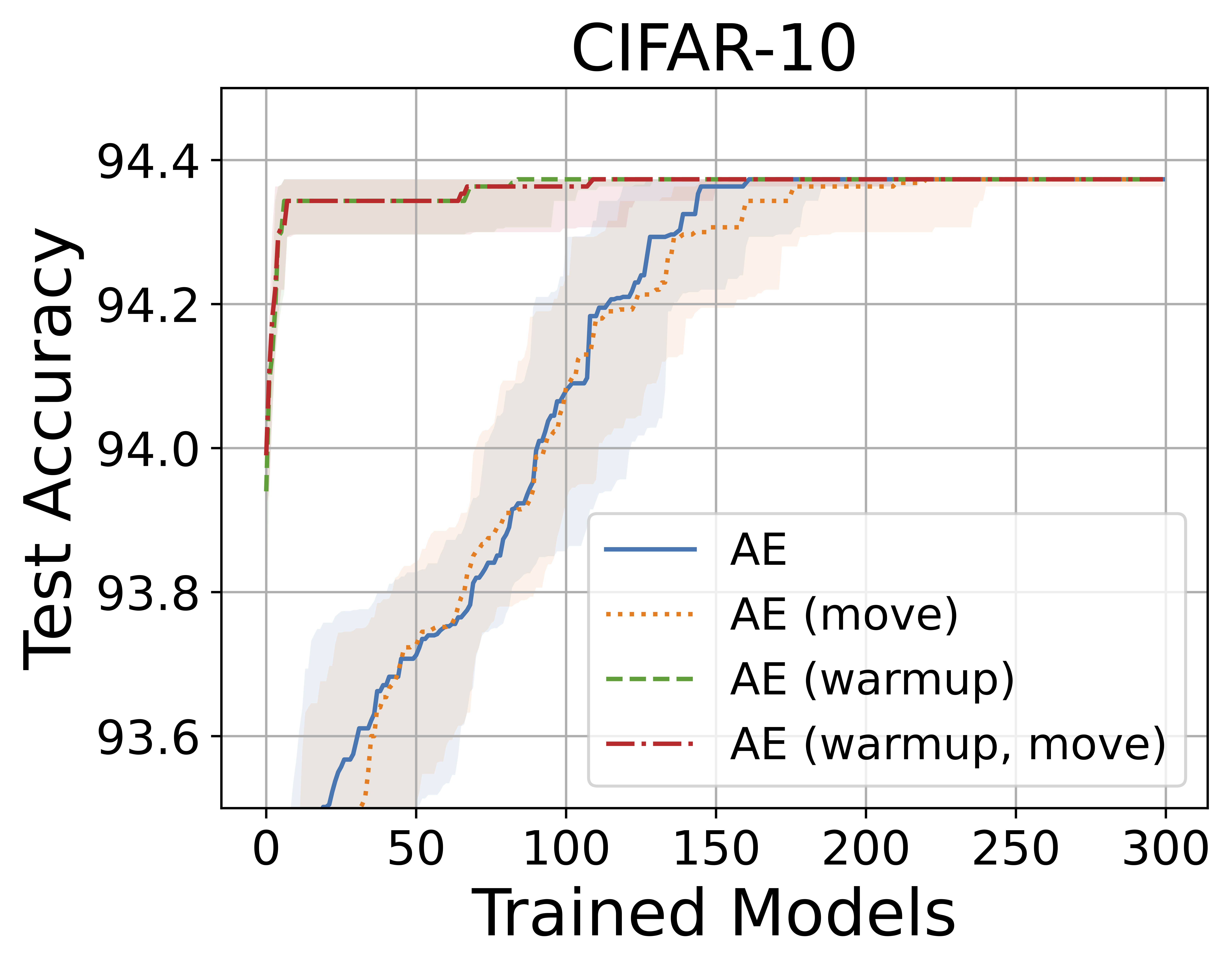
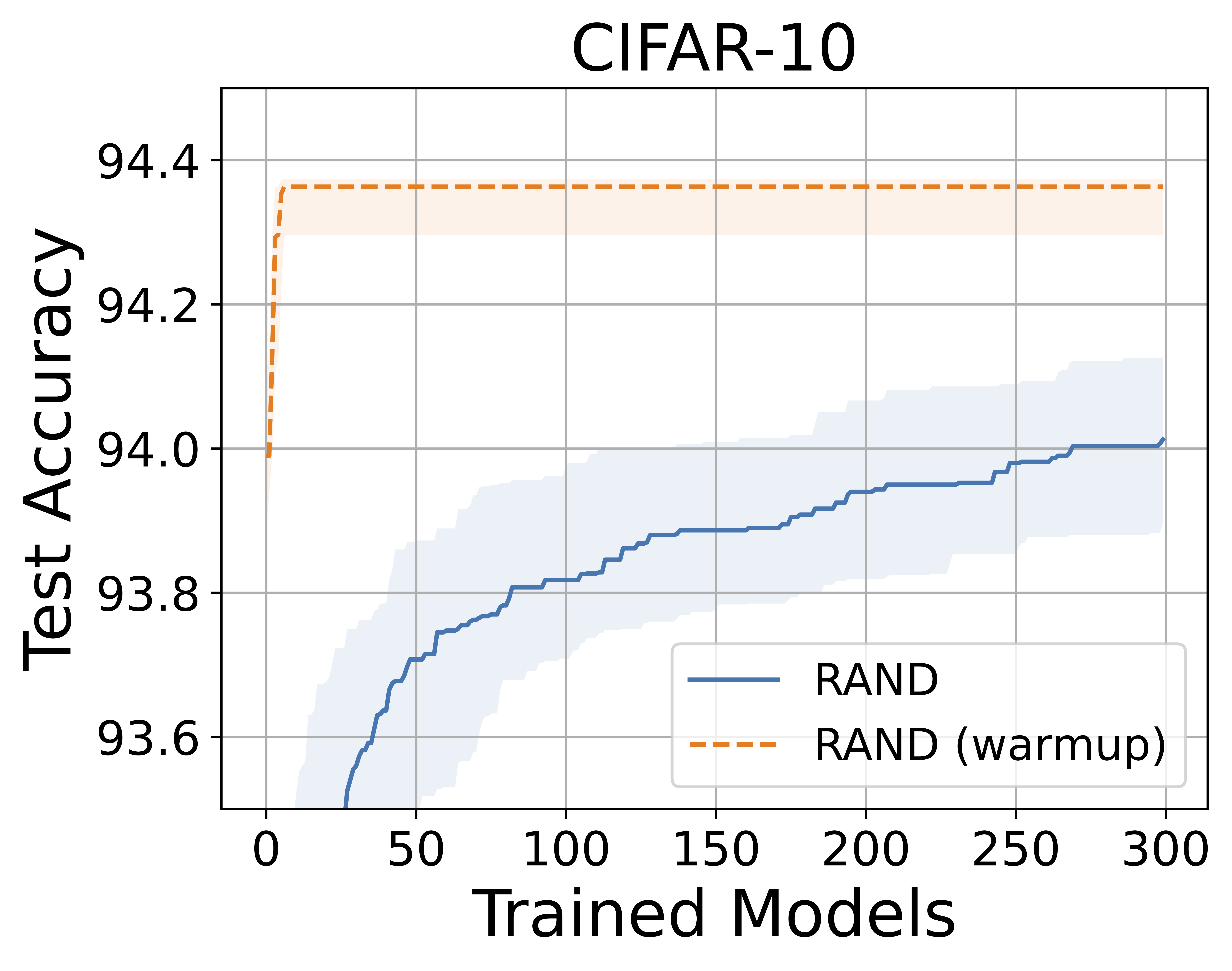
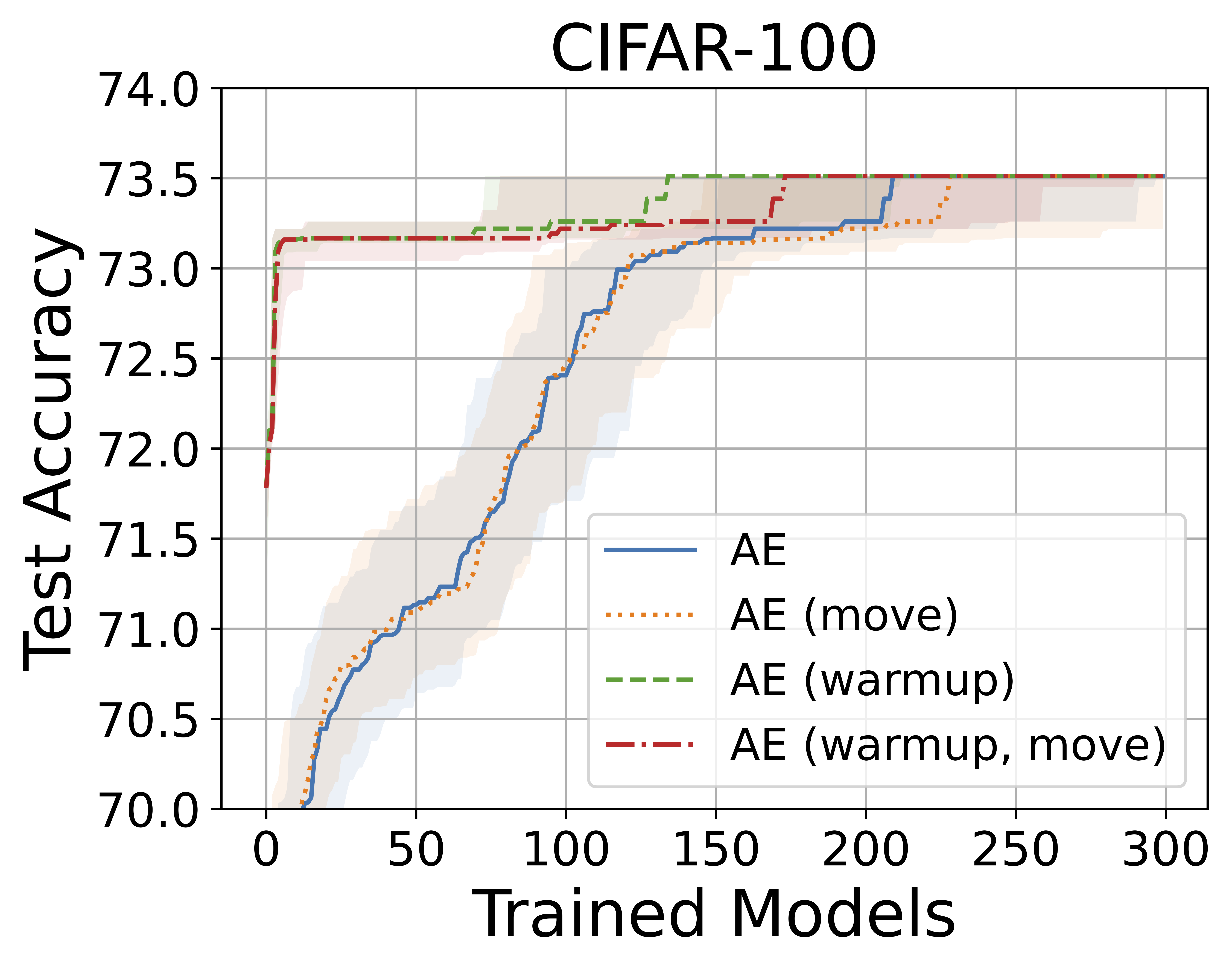
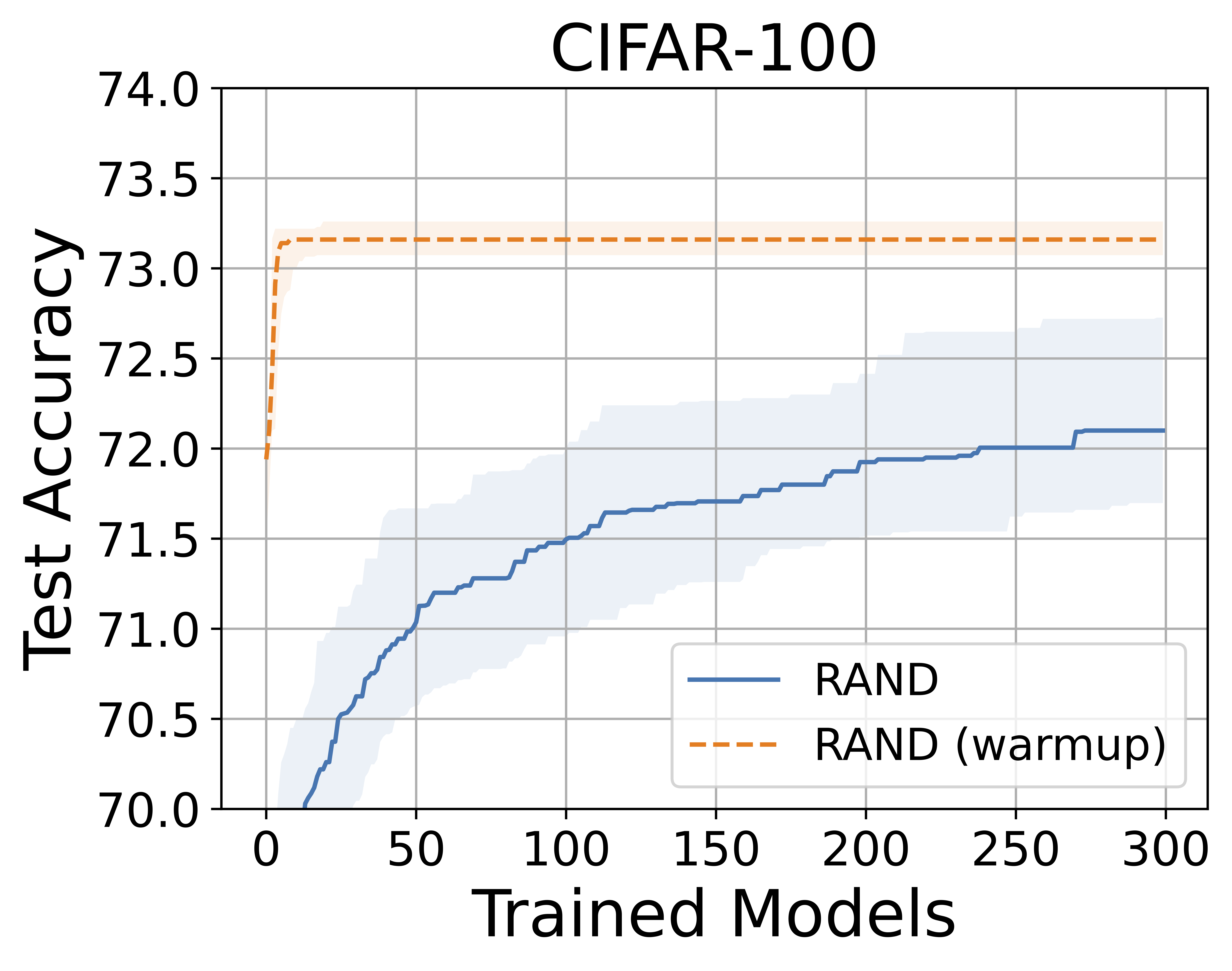
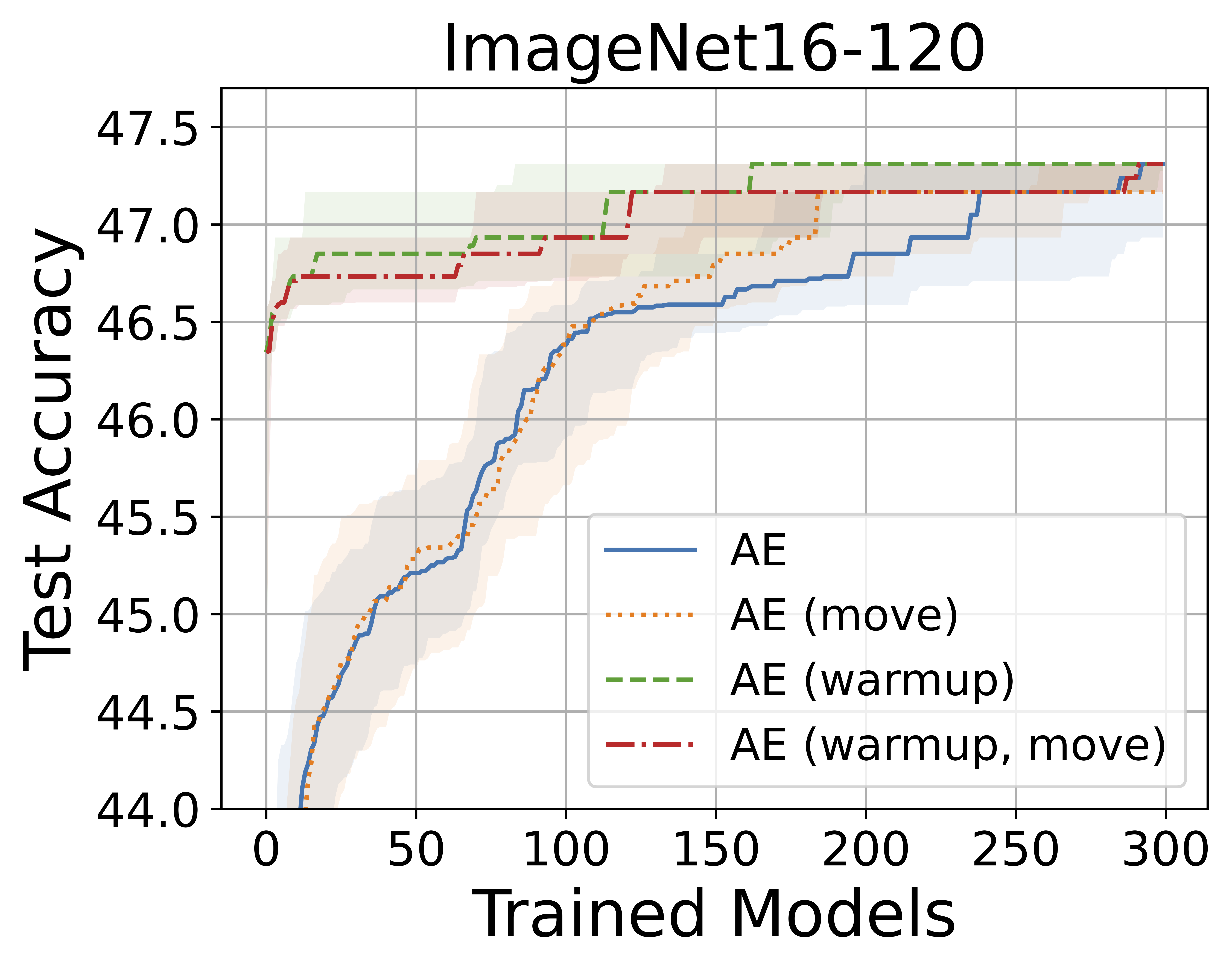
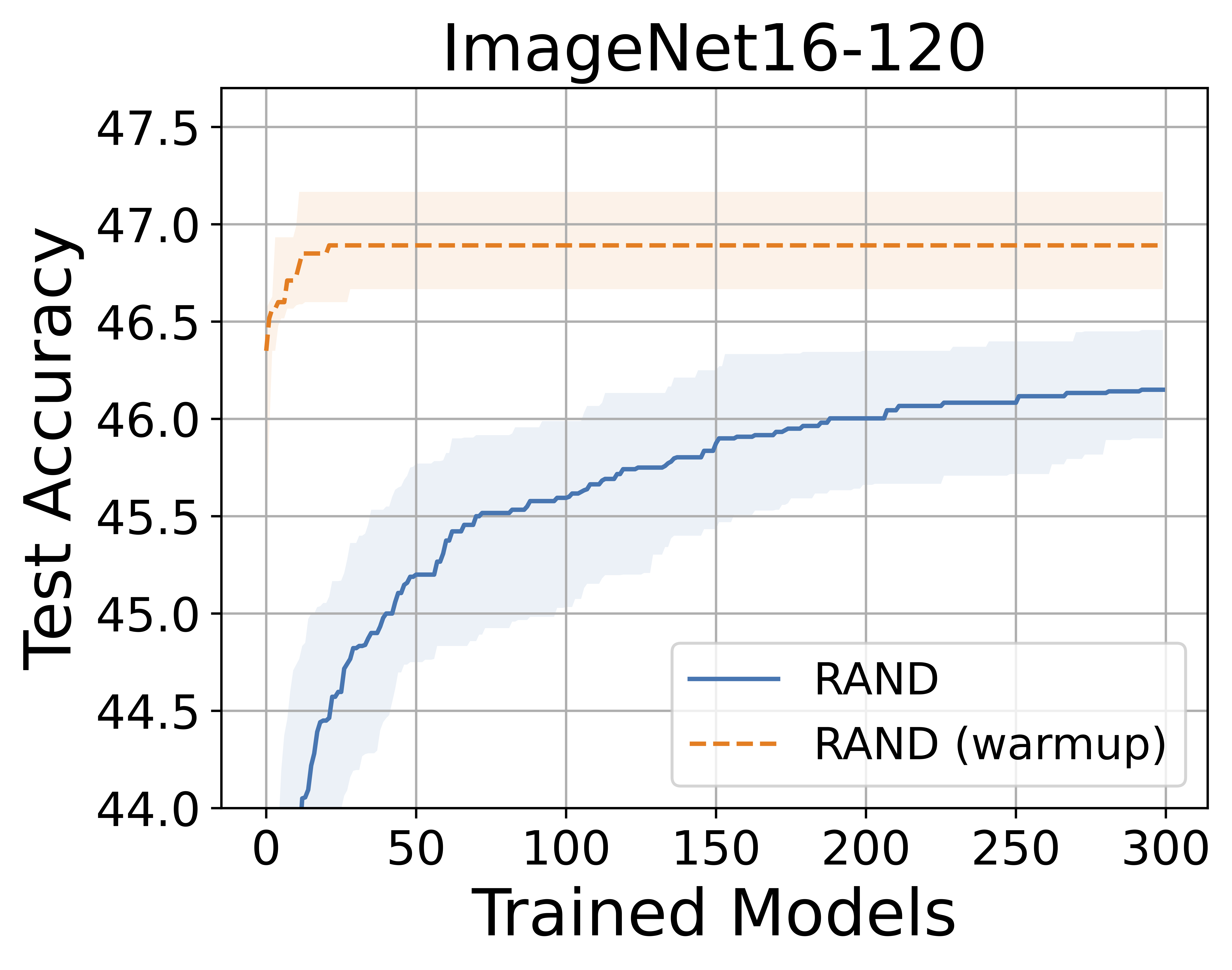
Figure 3: epsilon integration within ageing evolution (top) and random search (bottom) NAS algorithms for three datasets from NAS-Bench-201 search space.

4 Discussion

While epsilon metric shows solid empirical performance, the underlying reasons for this are unclear.

There are several hints towards its understanding. First, mathematically, epsilon represents the difference in the output distribution shapes between initialisations. The shape of the output is affected by layer widths, activation functions, batch normalisation, skip connections and other factors, which we generally refer to as network geometry. With constant shared weights, one can probe the effects of the geometry without being obstructed by the randomness of initialisation.

Second, during the weight ablation studies (Section A.1), we noticed that the best performance is achieved when the weights are set to the lowest and highest values that do not lead to excessive outputs explosion or vanishing. Therefore, epsilon measures the amplitude of the outputs’ distribution shape change due to geometry.

Finally, during the synthetic data studies, we see that grey-scale solid images work reasonably well as inputs. The distribution over the input samples is uniform, which makes it easier to track the changes in its shape as the signal propagates through the network.

That said, a coherent theoretical foundation of epsilon is missing and should be developed in future.

5 Conclusions

This work presents a novel zero-cost NAS scoring metric epsilon. It consists of two network initialisations followed by two forward passes. The value of epsilon reflects how neural network outputs’ distribution changes between low and high constant shared weight initialisations. It shows that the higher this difference, the better the network will perform upon training.

The metric does not require labels or gradient computation and is fast and lightweight. Evaluation takes $0.1\sim 1$ seconds per architecture on a single GPU (depending on the size of the architecture and batch size) and can be realised on a CPU. epsilon can virtually apply for any ML problem (care should be taken with embedding initialisation, as explained in Section A.1.4).

This work evaluates epsilon on three staple NAS search spaces: NAS-Bench-201, NAS-Bench-101 and NAS-Bench-NLP. It shows good stable performance with each of them, regardless of the data set. It also significantly improves the performances of random and evolutionary NAS algorithms (see Section 3.2).

The only significant disadvantage of the method is that it requires the choice of constant weight values during initialisation. Our tests show that it must be set up individually for each search space. We plan to automate the weight selection process in our future work.

Acknowledgments

The authors would like to thank Dr. Ayako Nakata and Dr. Guillaume Lambard for their continuous support and advice.

Appendix A Appendix

A.1 Ablation studies

While our metric is relatively straightforward to implement, it does require several hyperparameters to be set. In this section, we provide the ablations studies’ results and analyse them.

A.1.1 Weights

To compute the epsilon metric, we initialise the networks with two distinct constant shared weights. The question is: how to fix their values, and how does this choice affect the whole method?

To answer this question, we ran a series of tests with multiple pairs of weights. In pairs, it makes sense to set the first weight always greater than the second one. This consideration stems from the fact that epsilon is based on the mean absolute difference between two initialisations. Therefore, it will output the same score for [$w_{1}$, $w_{2}$] and [$w_{2}$, $w_{1}$] combinations and will be exactly zero in the case where the two weights are equal. Tables 5, 6, 7 summarises the results of our tests. For the NAS-Bench-201 search space, the outcomes are very similar between the datasets, and the minor differences do not affect the conclusions drawn from this data.

Table 5: Zero-cost metrics performance evaluated on NAS-Bench-101 search space, CIFAR-10 dataset. We start with $5{,}000$ randomly picked architectures. The number of architectures with non-NaN values are given in the second column.

Weights	Archs	Spearman $\rho$			Kendall $\tau$		Top-10%/	Top-64/
		global	top-10%		global	top-10%	top-10%	top-5%
0.0001, 0.001	2120	0.47	0.41		0.33	0.28	38.21	23
0.0001, 0.01	2120	0.61	0.03		0.43	0.02	41.98	24
0.0001, 0.1	2120	0.61	0.03		0.43	0.02	41.98	24
0.0001, 1	2120	0.61	0.03		0.43	0.02	41.98	24
0.0001, 10	2120	0.61	0.03		0.43	0.02	41.98	24
0.001, 0.01	4968	0.29	-0.05		0.20	-0.03	17.30	10
0.001, 0.1	4968	0.29	-0.05		0.19	-0.03	17.30	8
0.001, 1	4968	0.29	-0.05		0.19	-0.03	17.30	8
0.001, 10	4968	0.29	-0.05		0.19	-0.03	17.30	8
0.01, 0.1	5000	0.21	-0.12		0.14	-0.08	4.60	0
0.01, 1	5000	0.21	-0.12		0.14	-0.08	4.60	0
0.01, 10	5000	0.21	-0.12		0.14	-0.08	4.60	0
0.1, 1	5000	-0.47	0.04		-0.32	0.03	0.20	0
0.1, 10	5000	-0.45	0.00		-0.30	0.00	0.20	0
1, 10	5000	-0.44	0.01		-0.29	0.00	0.20	0

Table 6: Zero-cost metrics performance evaluated on NAS-Bench-201 search space, CIFAR-10 dataset. We start with $5{,}000$ randomly picked architectures. The number of architectures with non-NaN values are given in the second column.

Weights	Archs	Spearman $\rho$			Kendall $\tau$		Top-10%/	Top-64/
		global	top-10%		global	top-10%	top-10%	top-5%
1e-08, 1e-07	2957	0.27	-0.46		0.20	-0.37	0.00	3
1e-08, 1e-06	2957	0.42	-0.41		0.28	-0.30	4.39	1
1e-08, 1e-05	2957	0.43	-0.19		0.31	-0.13	9.12	2
1e-08, 0.0001	2957	0.47	-0.01		0.32	0.00	9.12	2
1e-08, 0.001	2957	0.62	0.06		0.43	0.05	18.92	3
1e-08, 0.01	2957	0.83	0.69		0.64	0.49	68.40	56
1e-08, 0.1	2957	0.84	0.64		0.65	0.46	68.03	56
1e-08, 1	2957	0.87	0.59		0.70	0.43	65.88	45
1e-08, 10	2957	0.87	0.58		0.70	0.43	66.78	46
1e-07, 1e-06	2957	0.33	-0.20		0.22	-0.13	4.76	1
1e-07, 1e-05	2957	0.39	-0.06		0.29	-0.04	9.15	2
1e-07, 0.0001	2957	0.47	-0.01		0.32	0.00	9.12	2
1e-07, 0.001	2957	0.62	0.06		0.43	0.05	18.92	3
1e-07, 0.01	2957	0.83	0.69		0.64	0.49	68.40	56
1e-07, 0.1	2957	0.84	0.64		0.65	0.46	68.03	56
1e-07, 1	2957	0.87	0.59		0.70	0.43	65.88	45
1e-07, 10	2957	0.87	0.58		0.70	0.43	66.78	46
1e-06, 1e-05	2957	0.41	-0.06		0.30	-0.04	9.15	2
1e-06, 0.0001	2957	0.47	-0.01		0.32	0.00	9.12	2
1e-06, 0.001	2957	0.62	0.06		0.43	0.05	18.92	3
1e-06, 0.01	2957	0.83	0.69		0.64	0.49	68.40	56
1e-06, 0.1	2957	0.84	0.64		0.65	0.46	68.03	56
1e-06, 1	2957	0.87	0.59		0.70	0.43	65.88	45
1e-06, 10	2957	0.87	0.58		0.70	0.43	66.78	46
1e-05, 0.0001	2957	0.47	-0.01		0.32	0.00	9.12	2
1e-05, 0.001	2957	0.62	0.06		0.43	0.05	18.92	3
1e-05, 0.01	2957	0.83	0.69		0.64	0.49	68.40	56
1e-05, 0.1	2957	0.84	0.64		0.65	0.46	68.03	56
1e-05, 1	2957	0.87	0.59		0.70	0.43	65.88	45
1e-05, 10	2957	0.87	0.58		0.70	0.43	66.78	46
0.0001, 0.001	2957	0.62	0.06		0.43	0.05	19.26	3
0.0001, 0.01	2957	0.82	0.69		0.63	0.49	68.42	56
0.0001, 0.1	2957	0.84	0.64		0.65	0.46	68.14	56
0.0001, 1	2957	0.87	0.58		0.69	0.42	65.88	46
0.0001, 10	2957	0.87	0.58		0.69	0.42	67.24	61
0.001, 0.01	4802	0.25	0.41		0.17	0.28	30.35	52
0.001, 0.1	4802	0.31	0.27		0.20	0.19	26.82	25
0.001, 1	4802	0.31	0.22		0.21	0.15	26.26	6
0.001, 10	4802	0.26	0.21		0.17	0.15	26.82	7
0.01, 0.1	4907	0.15	0.42		0.10	0.29	37.47	57
0.01, 1	4907	0.12	0.39		0.06	0.27	35.85	57
0.01, 10	4907	0.12	0.39		0.06	0.27	35.85	56
0.1, 1	4907	0.01	0.26		-0.03	0.16	0.84	0
0.1, 10	4907	0.01	0.26		-0.03	0.16	0.43	0
1, 10	4907	-0.02	0.25		-0.05	0.16	0.00	0

Table 7: Zero-cost metrics performance evaluated on NAS-Bench-NLP search space, PTB dataset. We start with $5{,}000$ randomly picked architectures. The number of architectures with non-NaN values are given in the second column.

Weights	Archs	Spearman $\rho$			Kendall $\tau$		Top-10%/	Top-64/
		global	top-10%		global	top-10%	top-10%	top-5%
1e-07, 1e-06	2393	-0.24	0.32		-0.16	0.22	0.00	0
1e-07, 1e-05	2391	-0.22	0.52		-0.15	0.39	1.67	0
1e-07, 0.0001	2388	-0.35	0.49		-0.24	0.37	0.42	1
1e-07, 0.001	2332	-0.42	0.50		-0.29	0.37	2.99	1
1e-07, 0.01	1215	-0.30	0.13		-0.21	0.09	4.20	1
1e-07, 0.1	585	-0.49	0.55		-0.36	0.44	1.69	1
1e-07, 1	403	-0.12	0.08		-0.08	-0.00	12.20	7
1e-06, 1e-05	3286	-0.11	0.49		-0.07	0.36	0.91	0
1e-06, 0.0001	3283	-0.24	0.47		-0.16	0.34	0.62	0
1e-06, 0.001	3226	-0.33	0.44		-0.23	0.33	4.64	1
1e-06, 0.01	1639	-0.26	0.13		-0.18	0.09	3.40	2
1e-06, 0.1	841	-0.41	0.13		-0.28	0.12	10.71	1
1e-06, 1	594	-0.09	0.13		-0.06	0.08	11.67	7
1e-05, 0.0001	3948	-0.32	0.30		-0.21	0.22	0.51	0
1e-05, 0.001	3892	-0.35	0.20		-0.24	0.16	3.85	2
1e-05, 0.01	1900	-0.32	0.27		-0.22	0.18	2.86	1
1e-05, 0.1	913	-0.38	0.31		-0.28	0.25	13.04	1
1e-05, 1	649	-0.18	0.36		-0.12	0.25	10.77	7
0.0001, 0.001	3987	-0.35	0.18		-0.24	0.14	3.76	0
0.0001, 0.01	1943	-0.37	0.38		-0.26	0.25	3.59	1
0.0001, 0.1	925	-0.43	0.26		-0.30	0.21	11.83	1
0.0001, 1	663	-0.26	0.35		-0.18	0.24	10.45	7
0.001, 0.01	1936	-0.32	0.40		-0.21	0.26	2.59	3
0.001, 0.1	918	-0.38	0.27		-0.30	0.22	8.70	2
0.001, 1	663	-0.23	-0.20		-0.19	-0.17	7.46	5
0.01, 0.1	910	-0.36	0.04		-0.25	0.02	8.79	2
0.01, 1	654	-0.25	0.06		-0.16	0.04	9.09	5
0.1, 1	652	-0.27	0.20		-0.19	0.13	10.61	7

The results show that there is indeed some variation between different initialisations. Two effects impact performance. Firstly, the more significant the difference between the two weights, the higher the correlation between epsilon and trained performance. It makes sense since if the weights are too close to each other, the difference between the outputs becomes minimal, and the distinction between architectures in terms of epsilon is no longer possible.

Secondly, we can see that too low and too high weights result in fewer architectures with non-NaN scores. Extreme weights result in all zeros or infinite output values and, consequently, in NaN value of the epsilon metric. Naturally, the deeper the network is, the more signal attenuation is, and the higher the probability of NaN score. We remind that prior to epsilon computation, the outputs are normalised to the same range $[0,1]$, which means the value of the metric per se does not become smaller for deeper networks. This extinction effect is due to the limited sensitivity of float type. Theoretically, with infinite float sensitivity, there would be no extinction and hence no effects on the choice of the weights.

Table 8: Optimal weights for epsilon evaluation for three search spaces and their datasets.

Search space	Dataset	Optimal weights
NAS-Bench-101	CIFAR-10	$[10^{-4},10]$
NAS-Bench-201	CIFAR-10	$[10^{-7},1]$
	CIFAR-100	$[10^{-7},1]$
	ImageNet16-120	$[10^{-7},1]$
NAS-Bench-NLP	PTB	$[10^{-5},10^{-3}]$

As a rule of thumb, for every new ML problem, we suggest running epsilon evaluation on a subset of architectures with several weights and selecting the minimum and maximum weights that do not cause excessive NaN outputs. While we acknowledge that this procedure is subjective, importantly, it does not require any training.

Weight combinations that we selected for each search space are given in Table 8.

A.1.2 Initialisation algorithm

The choice to initialise the weights with constant values provides a ground for discussion. On the one hand, constant shared weights guarantee the same initialisation regardless of the structure; the noise from the randomness of other initialisations is not obstructing the effect of the neural geometry. It would be possible to reduce the amount of noise by increasing the number of independent initialisations with distinct random seeds similar to the work of Gracheva [2021], but this increases the algorithm run-time proportionally.

Table 9 gives the results of the ablation studies when we compute epsilon based on two initialisations.

Table 9: Initialisations ablation studies. The metric is computed over $5{,}000$ initial architectures. The number of remaining architectures is given in the second column.

Initialisation	Archs	Spearman $\rho$			Kendall $\tau$		Top-10%/	Top-64/
		global	top-10%		global	top-10%	top-10%	top-5%
Uniform	15284	0.14	-0.17		0.09	-0.11	3.07	7
Normal	15284	0.44	-0.29		0.30	-0.20	20.07	4
Kaiming uniform	15284	0.32	0.11		0.21	0.07	27.40	26
Kaiming normal	15284	0.49	-0.29		0.33	-0.20	17.86	7
Orthogonal	15284	0.41	-0.20		0.28	-0.13	15.11	1

A.1.3 Batch size

To test the method’s sensitivity against the batch size, we ran the scoring routine with $8$ different batch sizes $[8,16,32,64,128,512,1024]$, each with $10$ random batches. The tests are done on the NAS-Bench-201 search space with its three datasets. For each batch, we report medians with $25$ and $75$ percentiles over $10$ runs. We evaluate epsilon on $5{,}000$ architectures.

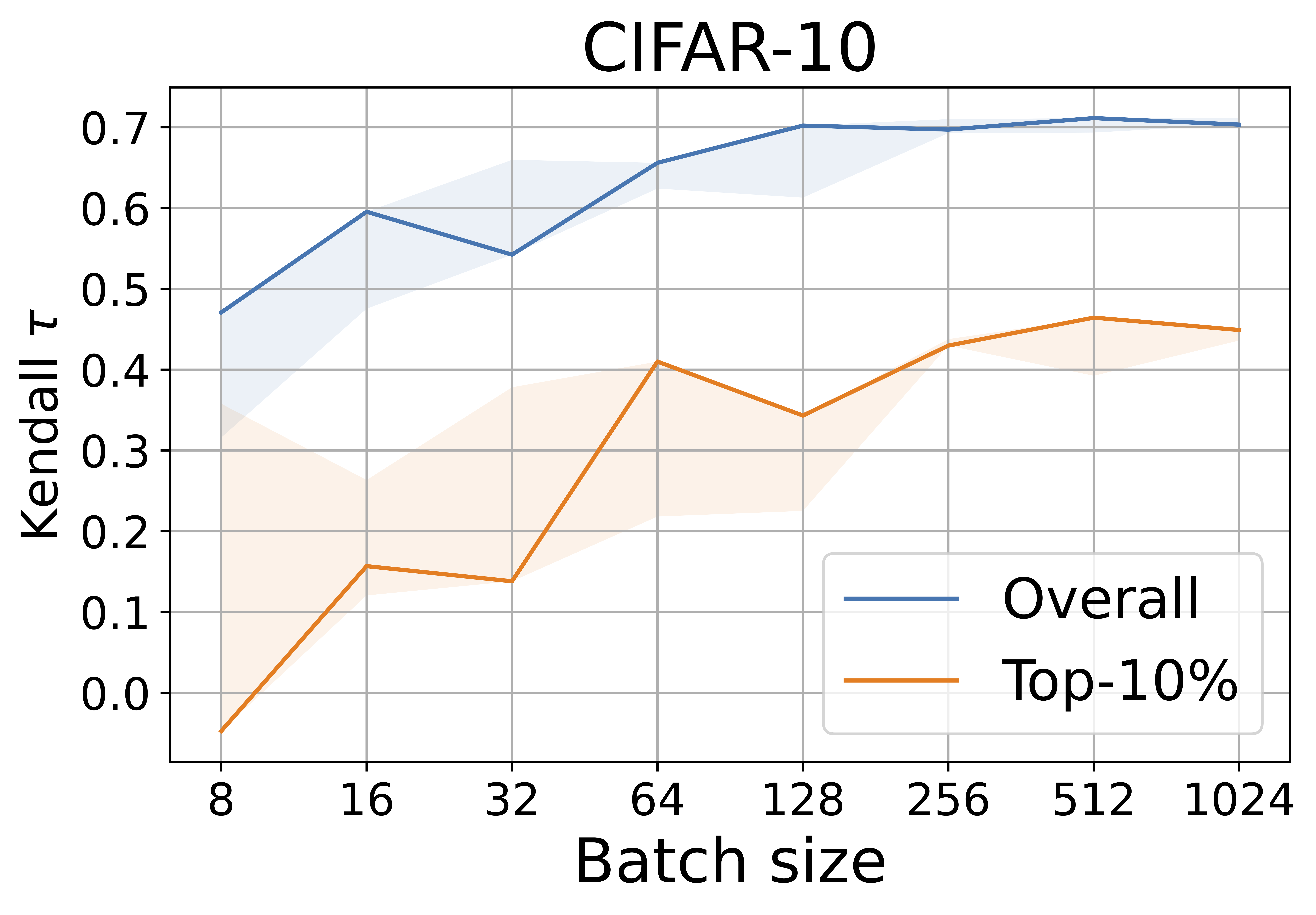
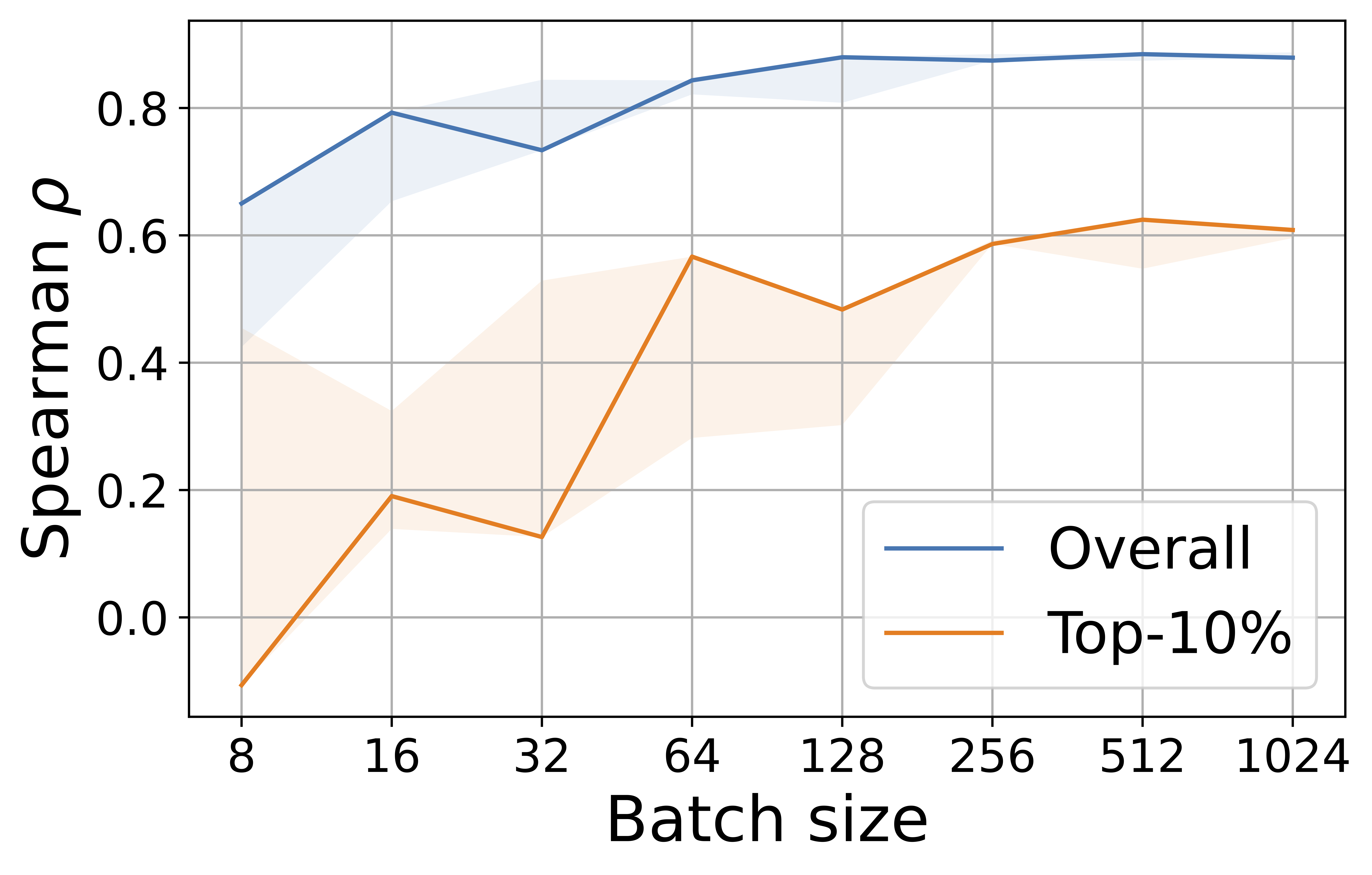
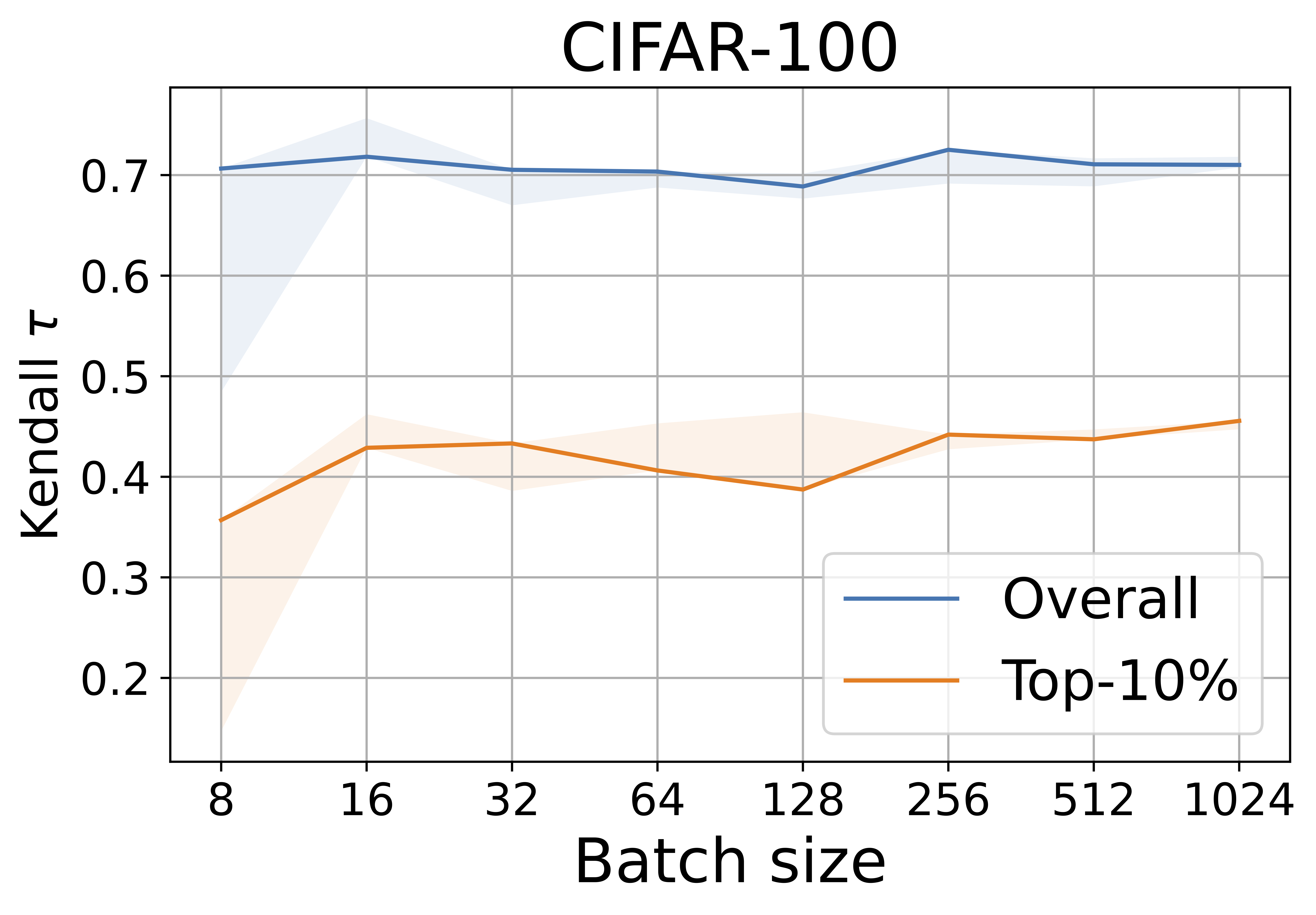
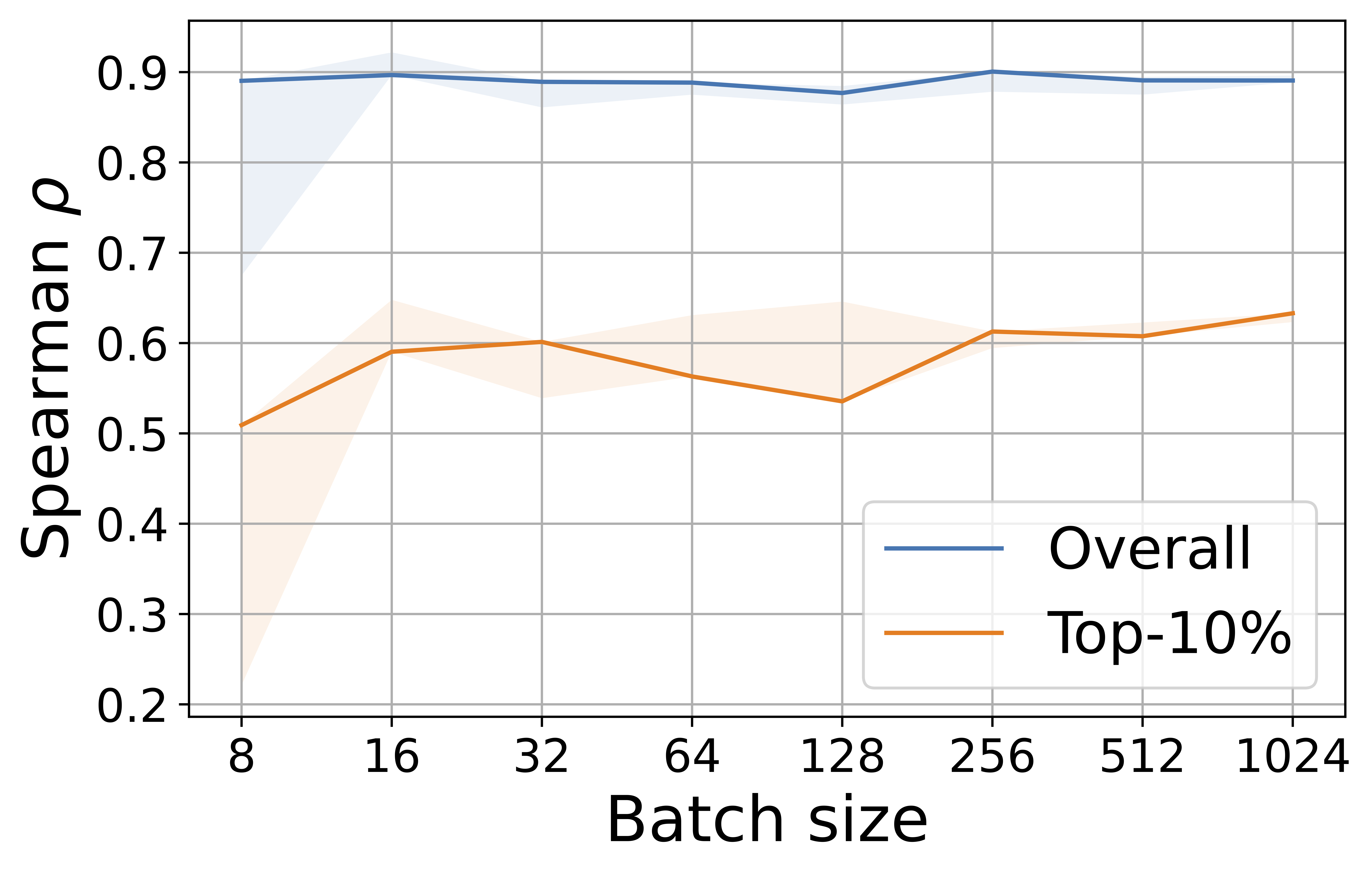
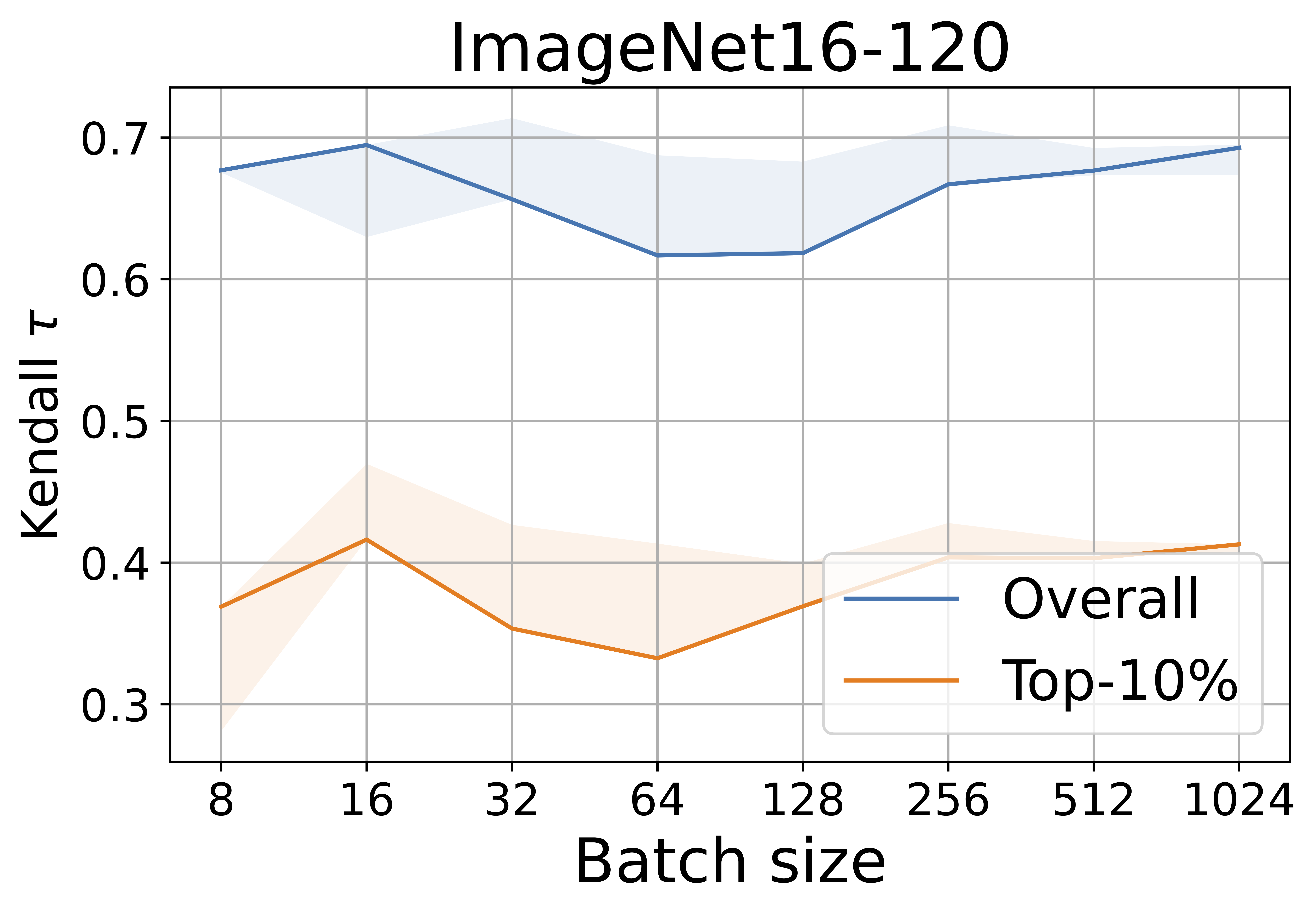
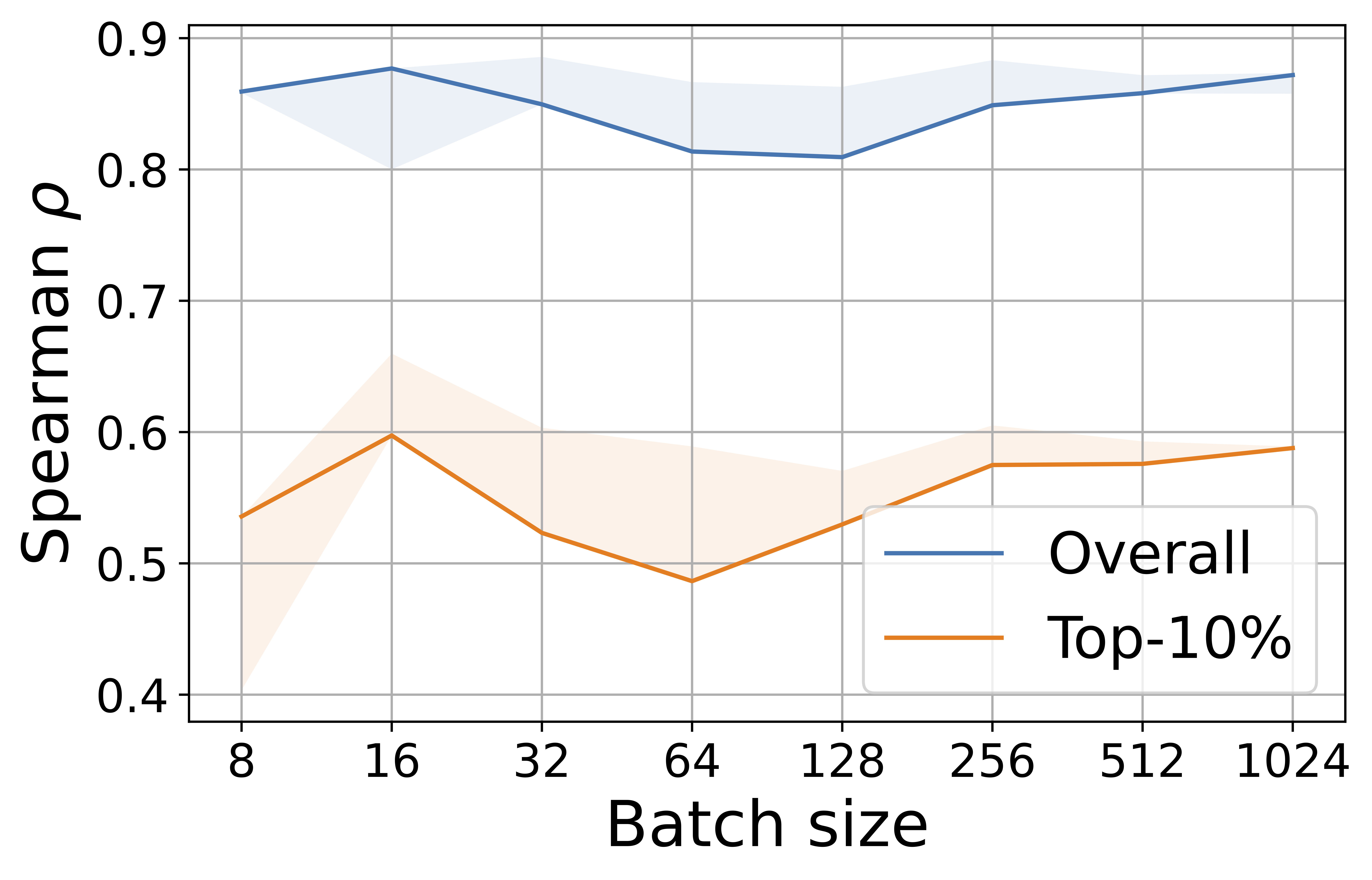
Figure 4: Batch size ablation study for NAS-Bench-201 search space, CIFAR-10 (left), CIFAR-100 (centre) and ImageNet16-120 (right) datasets.

Figure 4 show that, as expected, the larger the batch size, the better and more stable the performance of epsilon metric. There is almost no improvement for batches over $256$. We set the batch size to this value in the experiments throughout the paper.

A.1.4 Embedding initialisation

In order to verify the effect of the embedding initialisation, we have run tests with $6$ different initialisations:

• uniform positive 0.1: random uniform from ranges [0, 0.1]

• uniform positive 1: random uniform from ranges [0, 1]

• uniform centred 0.1: random uniform from ranges [-0.1, 0.1]

• uniform centred 1: random uniform from ranges [-1, 1]

• random 0.1: random normal centred at $0$ with a standard deviation of 0.1

• random 1: random normal centred at $0$ with a standard deviation of 1

Table 10 summarises our results of the embedding ablations. Ablation is done on the NAS-Bench-NLP search space, PTB dataset (the only search space implementing embedding).

Table 10: Embedding ablation studies. Metric computed over $5{,}000$ initial architectures. The number of remaining architectures is given in the second column.

Embedding	Archs	Spearman $\rho$			Kendall $\tau$		Top-10%/	Top-64/
		global	top-10%		global	top-10%	top-10%	top-5%
uniform positive 0.1	782	-0.38	0.17		-0.26	0.15	3.80	2
uniform positive 1	776	-0.37	0.21		-0.26	0.18	2.56	2
uniform centered 0.1	783	-0.40	0.18		-0.28	0.15	2.53	2
uniform centered 1	782	-0.46	0.18		-0.33	0.16	1.27	1
random 0.1	783	-0.42	0.18		-0.29	0.15	2.53	2
random 1	782	-0.47	0.19		-0.33	0.16	1.27	1

Care should be taken when initialising the networks containing the embedding layer: if embedding is initialised with all constants, there is no difference between the embedded input. The performance of our metric, in this case, will be analogous to that with a batch size of one.

Our ablation studies show that as soon as the embedding is initialised with non-constant weights, it does not significantly influence the outcomes.

A.1.5 Synthetic data

In this section, we test the importance of the input data by feeding our metric several synthetic input data on CIFAR-10. We feed networks with $5$ types of data:

• actual data: a batch of CIFAR-10 data

• grey scale images: images within the batch are solid colour ranging from black to white

• random normal: images are filled with random values following normal distribution with $[\mu,\sigma]=[0,1]$

• random uniform: images are filled with random values following uniform distribution with $[\mu,\sigma]=[-1,1]$

• random uniform (+): images are filled with random values following uniform distribution with $[min,\max]=[0,1]$

All the tests are performed with batch size of $256$, weights $[10^{-7},1]$ and $5{,}000$ architectures. Table 11 shows that even though the performance with synthetic data drops compared to actual data, it is still reasonably good.

Curiously, greyscale images, filled with constant values, show the closest results to the actual data. Note that epsilon metric with greyscale data outperforms synflow. It is an essential achievement because synflow does not use input data and is, therefore, data independent. Our results show that epsilon has the potential to be used with no data whatsoever.

Table 11: Synthetic data tests with CIFAR-10 dataset, NAS-Bench-201 search space. Tests are based on the evaluation of $5{,}000$ architectures.

Metric	Spearman $\rho$			Kendall $\tau$		Top-10%/	Top-64/
	global	top-10%		global	top-10%	top-10%	top-5%
real data	0.87	0.59		0.70	0.43	65.88	$45$
grey scale	0.87	0.44		0.68	0.31	59.46	$34$
random normal	0.54	0.15		0.38	0.14	14.97	$3$
random uniform	0.56	0.17		0.40	0.16	14.19	$3$
random uniform (+)	0.61	0.17		0.43	0.16	16.22	$4$

A.2 Visualisation of other zero-cost NAS metrics

A.2.1 When integrated with other NAS methods

In Section 3.2, we show how epsilon metric improves the performance of ageing evolution and random search when used for warming up. Figure 5 compares epsilon integration to other metrics from Abdelfattah et al. [2021]. For both EA ans RS, we use the metrics for a warm-up and run the procedure until the number of trained architectures reaches $300$ with $100$ random rounds. The warm-up pool contains $3000$ randomly selected architectures.

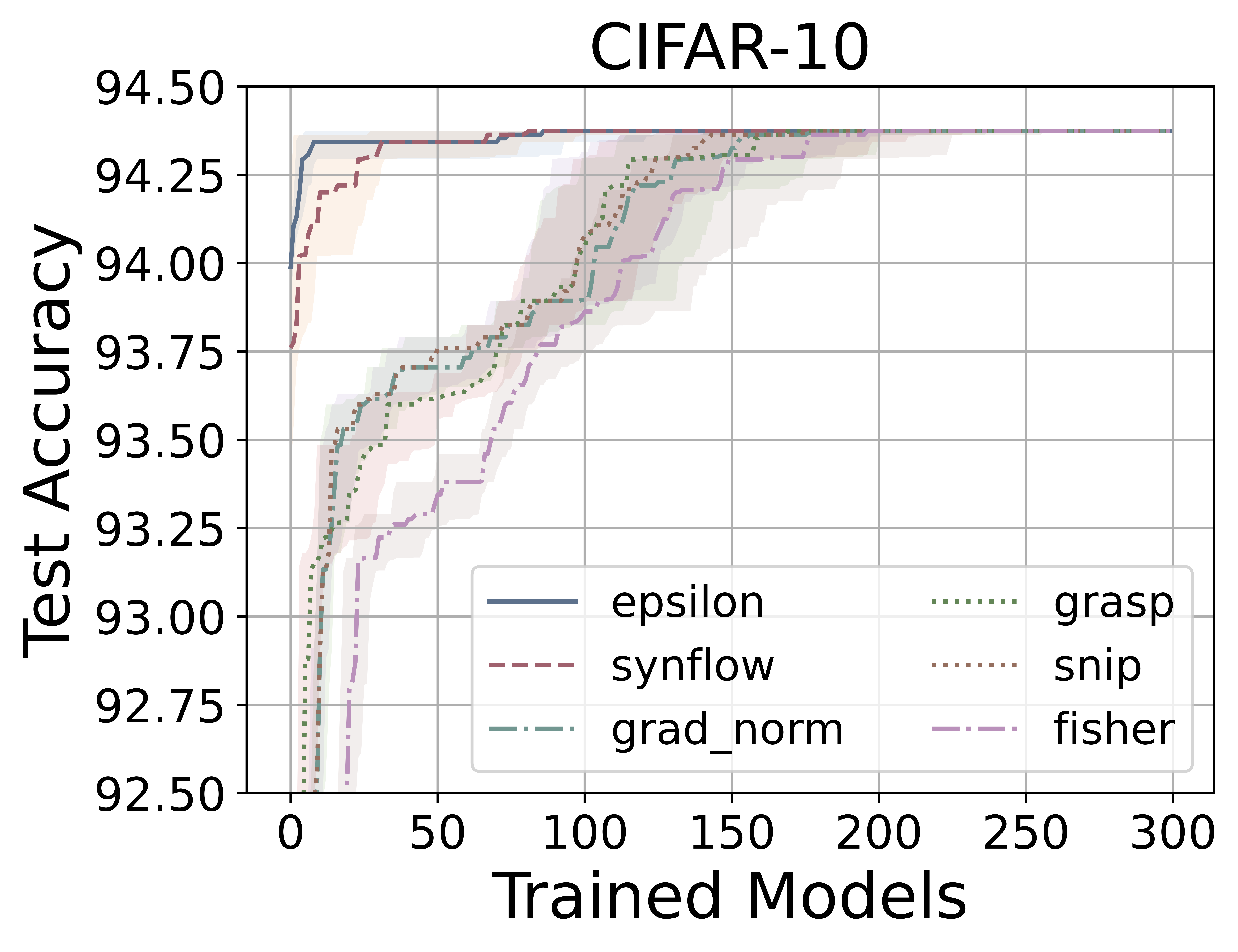
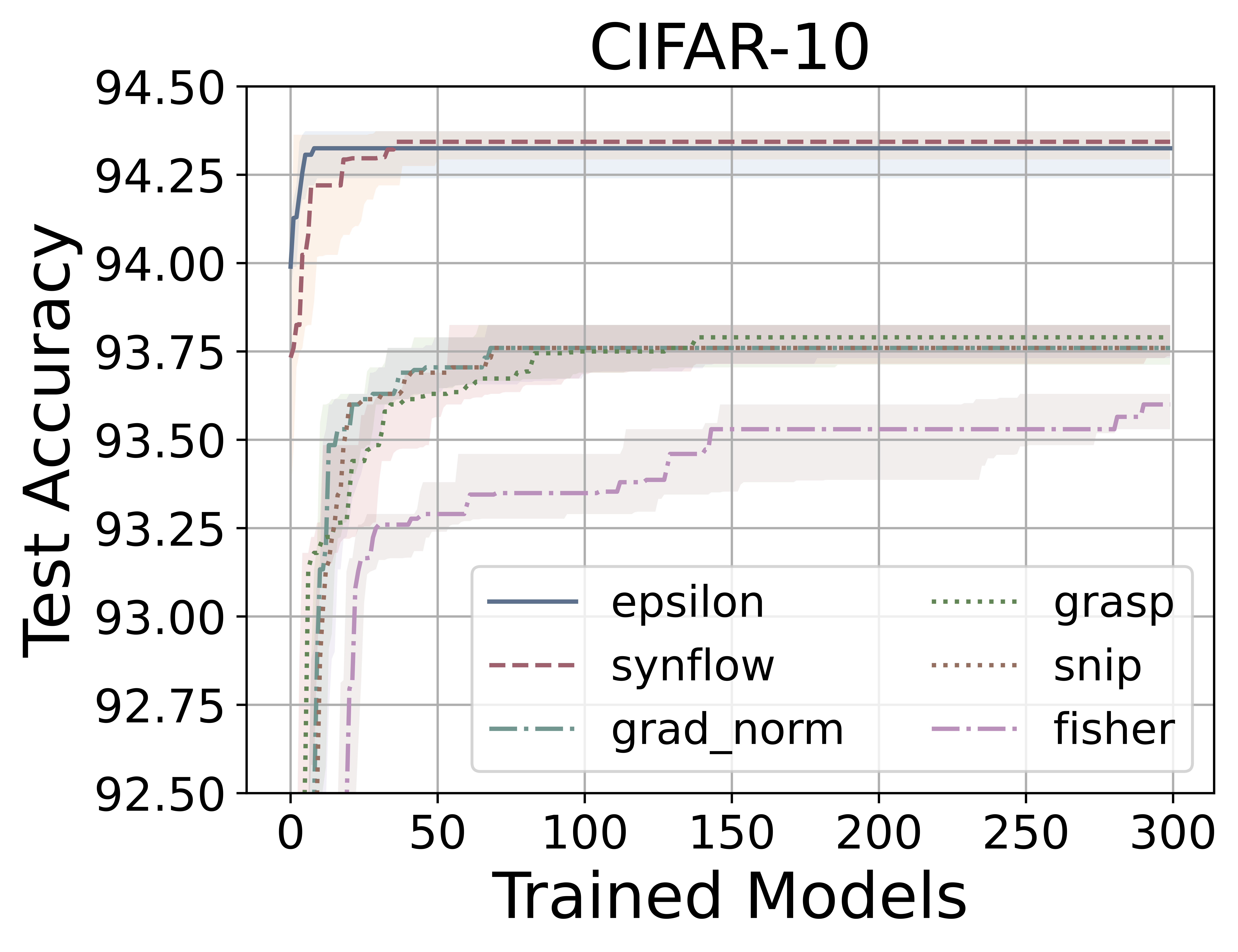
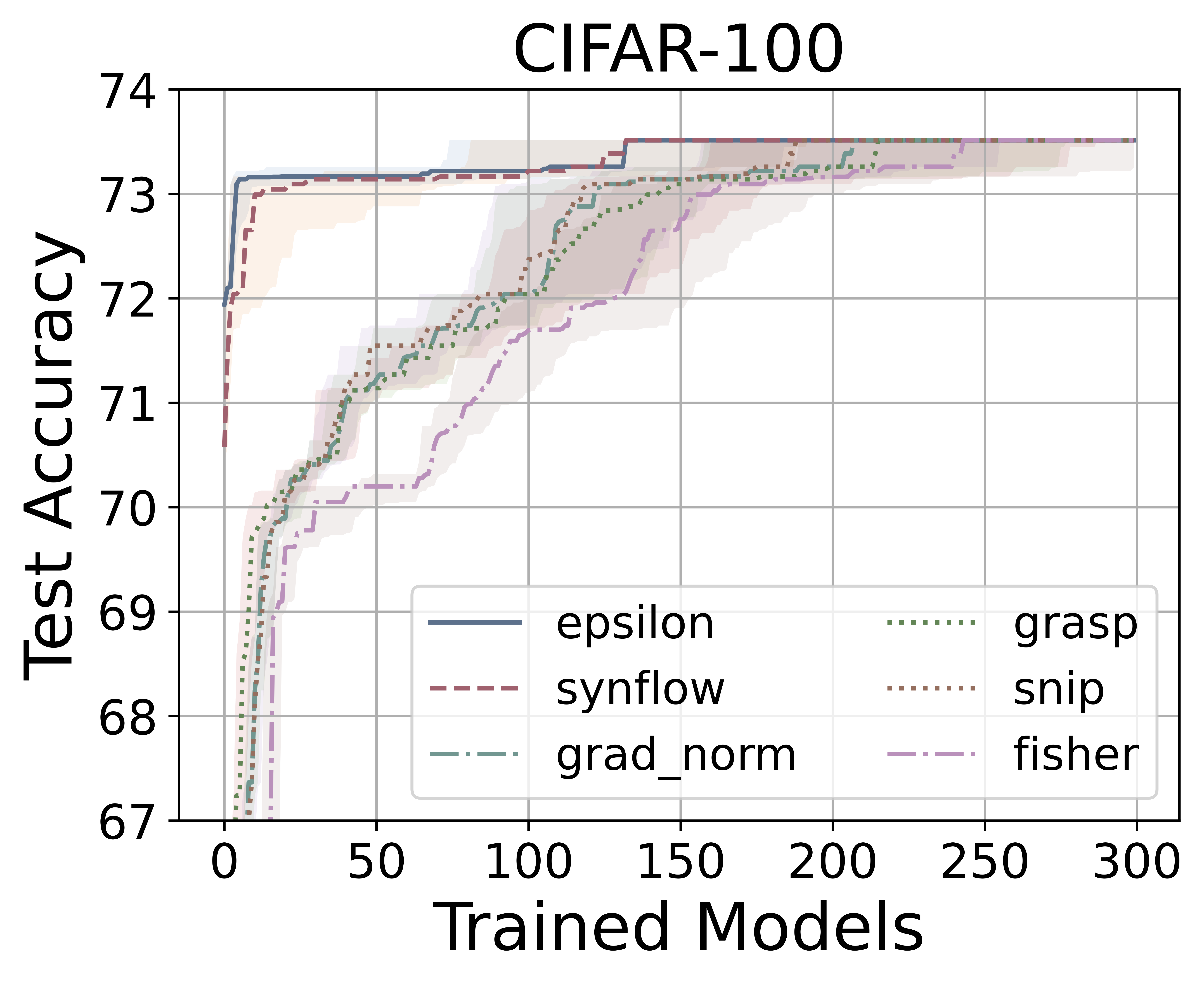
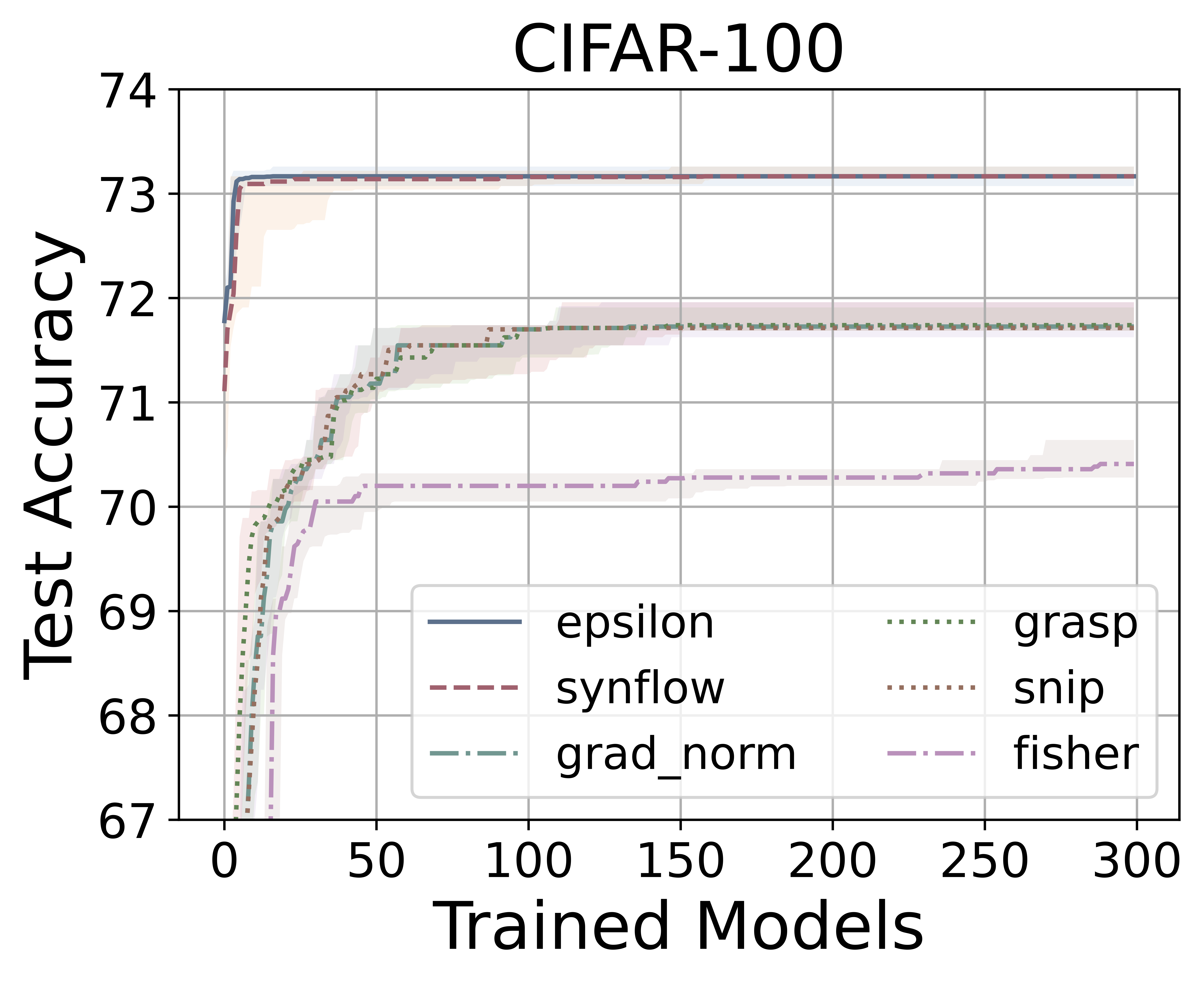
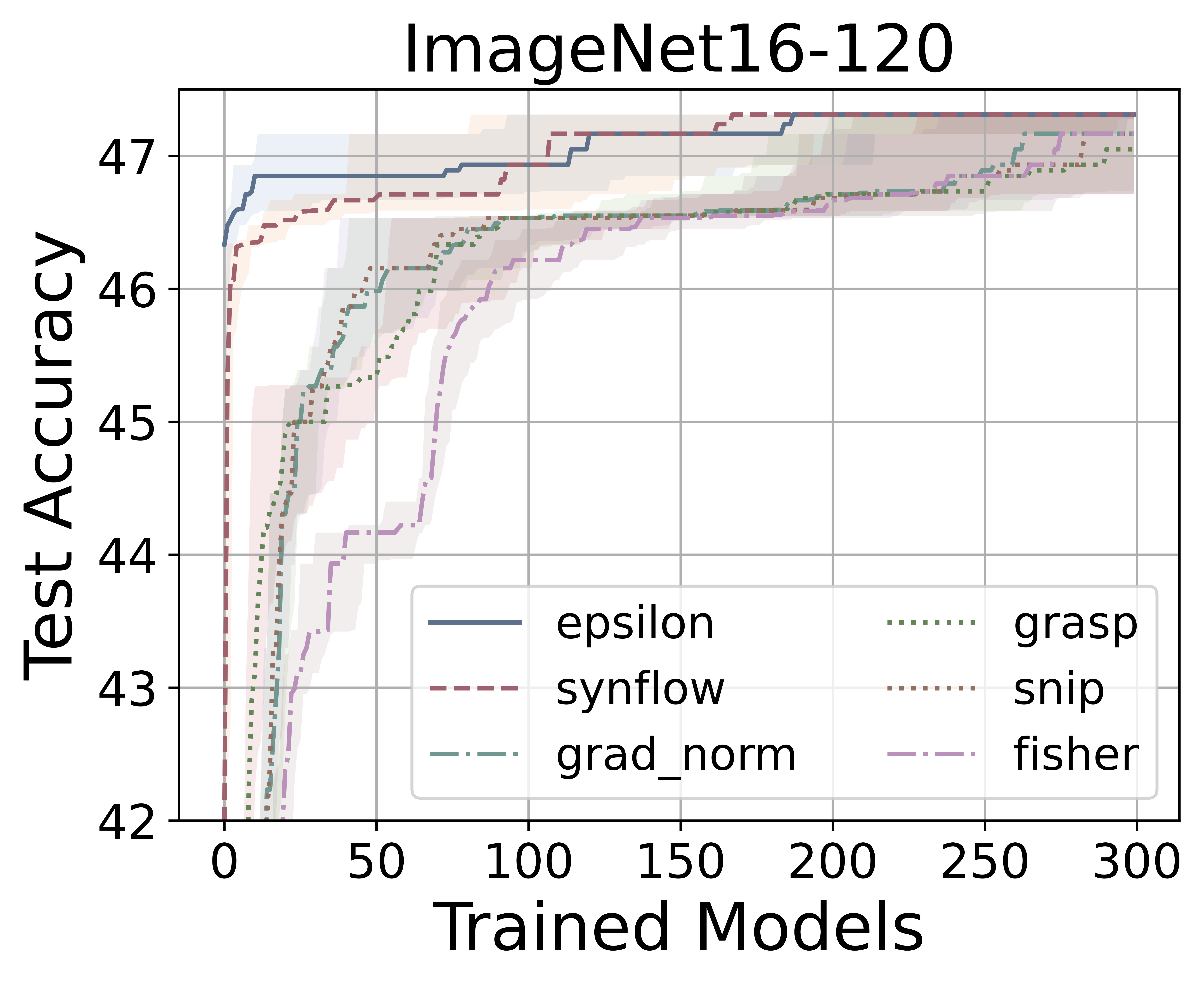
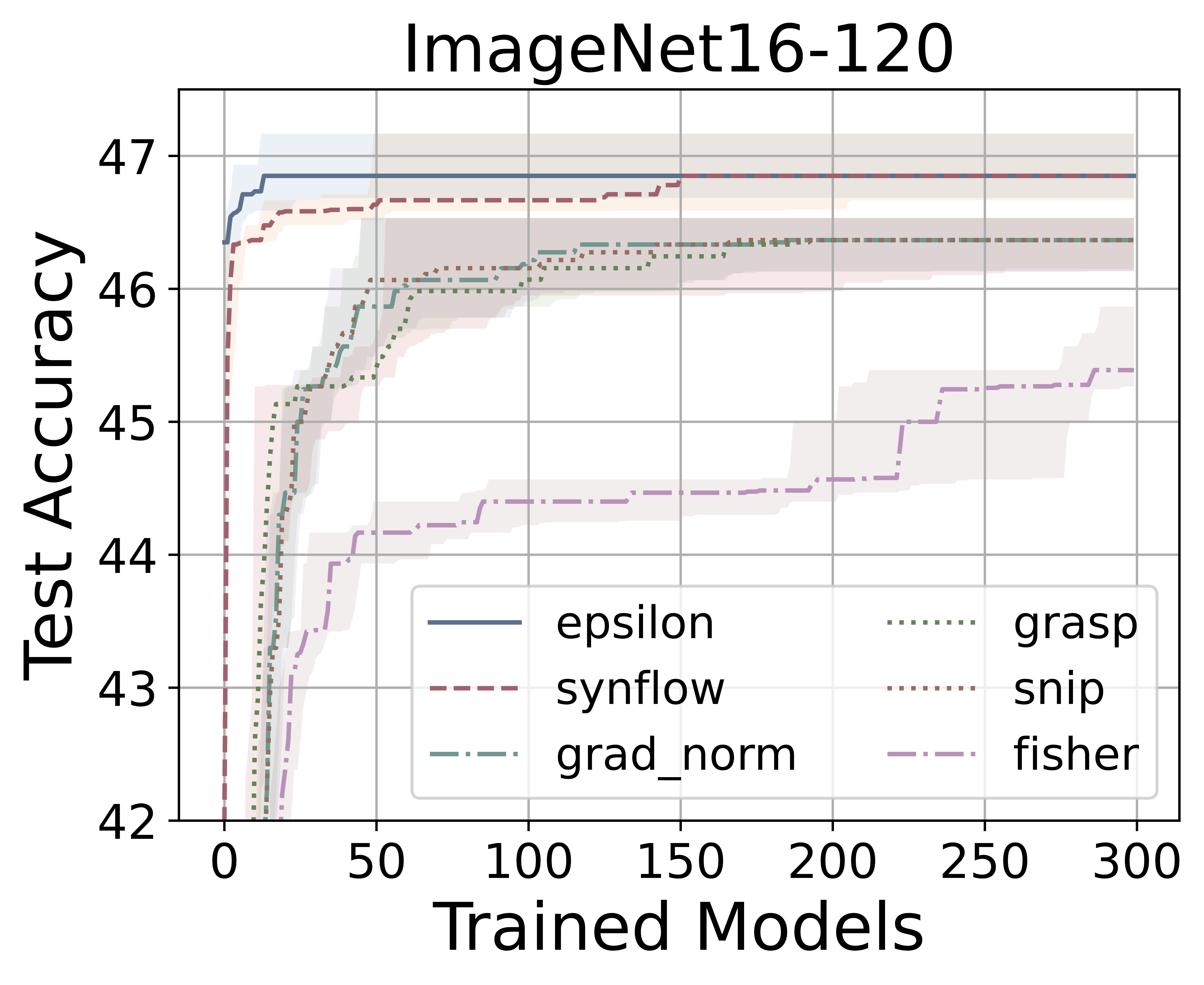
Figure 5: Various zero-cost NAS metrics’ performance when used as a warm-up for ageing evolution (top) and random search (bottom) for three datasets from the NAS-Bench-201 search space. Shadows span between lower and upper quartiles based on $100$ rounds. The warm-up population is $3000$ architectures.

A.2.2 Correlation with accuracy

In the work of Abdelfattah et al. [2021] the metrics are presented through statistical measures, but we feel that visualisation helps to improve understanding. Here we provide visualisations for two search spaces built on the data provided by the authors.

References

- Williams [1992] Ronald J Williams. Simple statistical gradient-following algorithms for connectionist reinforcement learning. Machine learning, 8(3):229–256, 1992.
- Real et al. [2019] Esteban Real, Alok Aggarwal, Yanping Huang, and Quoc V Le. Regularized evolution for image classifier architecture search. In Proceedings of the aaai conference on artificial intelligence, volume 33, pages 4780–4789, 2019.
- Falkner et al. [2018] Stefan Falkner, Aaron Klein, and Frank Hutter. Bohb: Robust and efficient hyperparameter optimization at scale. arXiv preprint arXiv:1807.01774, 2018.
- White et al. [2021] Colin White, Willie Neiswanger, and Yash Savani. Bananas: Bayesian optimization with neural architectures for neural architecture search. In Proceedings of the AAAI Conference on Artificial Intelligence, volume 35, pages 10293–10301, 2021.
- Pham et al. [2018] Hieu Pham, Melody Y Guan, Barret Zoph, Quoc V Le, and Jeff Dean. Efficient neural architecture search via parameter sharing. arXiv preprint arXiv:1802.03268, 2018.
- Li and Talwalkar [2020] Liam Li and Ameet Talwalkar. Random search and reproducibility for neural architecture search. In Uncertainty in artificial intelligence, pages 367–377. PMLR, 2020.
- Dong and Yang [2019] Xuanyi Dong and Yi Yang. Searching for a robust neural architecture in four gpu hours. In Proceedings of the IEEE/CVF Conference on Computer Vision and Pattern Recognition, pages 1761–1770, 2019.
- Chu et al. [2020] Xiangxiang Chu, Xiaoxing Wang, Bo Zhang, Shun Lu, Xiaolin Wei, and Junchi Yan. Darts-: robustly stepping out of performance collapse without indicators. arXiv preprint arXiv:2009.01027, 2020.
- Istrate et al. [2019] Roxana Istrate, Florian Scheidegger, Giovanni Mariani, Dimitrios Nikolopoulos, Constantine Bekas, and Adelmo Cristiano Innocenza Malossi. Tapas: Train-less accuracy predictor for architecture search. In Proceedings of the AAAI Conference on Artificial Intelligence, volume 33, pages 3927–3934, 2019.
- Deng et al. [2017] Boyang Deng, Junjie Yan, and Dahua Lin. Peephole: Predicting network performance before training. arXiv preprint arXiv:1712.03351, 2017.
- Northcutt et al. [2021] Curtis G Northcutt, Anish Athalye, and Jonas Mueller. Pervasive label errors in test sets destabilize machine learning benchmarks. arXiv preprint arXiv:2103.14749, 2021.
- Gaier and Ha [2019] Adam Gaier and David Ha. Weight agnostic neural networks. Advances in neural information processing systems, 32, 2019.
- LeCun et al. [2010] Yann LeCun, Corinna Cortes, and CJ Burges. Mnist handwritten digit database. ATT Labs [Online]. Available: http://yann.lecun.com/exdb/mnist, 2, 2010.
- Mellor et al. [2020] Joseph Mellor, Jack Turner, Amos Storkey, and Elliot J Crowley. Neural architecture search without training. arXiv preprint arXiv:2006.04647v1, 2020.
- Agarap [2018] Abien Fred Agarap. Deep learning using rectified linear units (relu). arXiv preprint arXiv:1803.08375, 2018.
- Abdelfattah et al. [2021] Mohamed S Abdelfattah, Abhinav Mehrotra, Łukasz Dudziak, and Nicholas D Lane. Zero-cost proxies for lightweight nas. arXiv preprint arXiv:2101.08134, 2021.
- Chen et al. [2021] Wuyang Chen, Xinyu Gong, and Zhangyang Wang. Neural architecture search on imagenet in four gpu hours: A theoretically inspired perspective. arXiv preprint arXiv:2102.11535, 2021.
- Gracheva [2021] Ekaterina Gracheva. Trainless model performance estimation based on random weights initialisations for neural architecture search. Array, 12:100082, 2021. ISSN 2590-0056. doi:https://doi.org/10.1016/j.array.2021.100082.
- Zhang and Jia [2021] Zhihao Zhang and Zhihao Jia. Gradsign: Model performance inference with theoretical insights. arXiv preprint arXiv:2110.08616, 2021.
- Wang et al. [2020] Chaoqi Wang, Guodong Zhang, and Roger Grosse. Picking winning tickets before training by preserving gradient flow. arXiv preprint arXiv:2002.07376, 2020.
- Lee et al. [2018] Namhoon Lee, Thalaiyasingam Ajanthan, and Philip HS Torr. Snip: Single-shot network pruning based on connection sensitivity. arXiv preprint arXiv:1810.02340, 2018.
- Tanaka et al. [2020] Hidenori Tanaka, Daniel Kunin, Daniel L Yamins, and Surya Ganguli. Pruning neural networks without any data by iteratively conserving synaptic flow. Advances in Neural Information Processing Systems, 33:6377–6389, 2020.
- Ying et al. [2019] Chris Ying, Aaron Klein, Eric Christiansen, Esteban Real, Kevin Murphy, and Frank Hutter. Nas-bench-101: Towards reproducible neural architecture search. In International Conference on Machine Learning, pages 7105–7114. PMLR, 2019.
- Krizhevsky et al. [2009] Alex Krizhevsky, Geoffrey Hinton, et al. Learning multiple layers of features from tiny images. Master’s thesis, Department of Computer Science, University of Toronto, 2009.
- Dong and Yang [2020] Xuanyi Dong and Yi Yang. Nas-bench-201: Extending the scope of reproducible neural architecture search. arXiv preprint arXiv:2001.00326, 2020.
- Chrabaszcz et al. [2017] Patryk Chrabaszcz, Ilya Loshchilov, and Frank Hutter. A downsampled variant of imagenet as an alternative to the cifar datasets. arXiv preprint arXiv:1707.08819, 2017.
- Klyuchnikov et al. [2022] Nikita Klyuchnikov, Ilya Trofimov, Ekaterina Artemova, Mikhail Salnikov, Maxim Fedorov, Alexander Filippov, and Evgeny Burnaev. Nas-bench-nlp: neural architecture search benchmark for natural language processing. IEEE Access, 10:45736–45747, 2022.
- Marcinkiewicz [1994] Mary Ann Marcinkiewicz. Building a large annotated corpus of english: The penn treebank. Using Large Corpora, 273, 1994.