Extended Decoupled Anisotropic Solutions in $f(\mathcal{R},\mathcal{T},\mathcal{R}_{\gamma\chi}\mathcal{T}^{\gamma\chi})$ Gravity

Abstract

In this paper, we consider static spherical structure to develop some anisotropic solutions by employing the extended gravitational decoupling scheme in the background of $f(\mathcal{R},\mathcal{T},\mathcal{R}_{\gamma\chi}\mathcal{T}^{\gamma\chi})$ gravity, where $\mathcal{R}$ and $\mathcal{T}$ indicate the Ricci scalar and trace of the energy-momentum tensor, respectively. We transform both radial as well as temporal metric functions and apply them on the field equations that produce two different sets corresponding to the decoupling parameter $\xi$. The first set is associated with isotropic distribution, i.e., modified Krori-Barua solution. The second set is influenced from anisotropic factor and contains unknowns which are determined by taking some constraints. The impact of decoupling parameter is then analyzed on the obtained physical variables and anisotropy. We also investigate energy conditions and some other parameters such as mass, compactness and redshift graphically. It is found that our solution corresponding to pressure-like constraint shows stable behavior throughout in this gravity for the considered range of $\xi$.

Keywords: $f(\mathcal{R},\mathcal{T},\mathcal{R}_{\gamma\chi}\mathcal{T}^{\gamma\chi})$ gravity; Gravitational decoupling; Anisotropy; Self-gravitating systems.
PACS: 04.50.Kd; 04.40.Dg; 04.40.-b.

1 Introduction

The structure of our cosmos is well-organized yet unfathomable, made up of massive geometrical structures such as stars and galaxies as well as other obscure components. The physical behavior of such heavily bodies help to understand cosmic evolution. General Relativity (GR) is the first relativistic theory which provides basic understanding of both astrophysical as well as cosmological phenomena. Numerous cosmological experiments performed on the far away galaxies indicate that our universe is getting larger rapidly. The repulsive form of energy, named as the dark energy, is considered to execute such expansion. The modifications to GR have therefore been found very important to disclose hidden features of our universe. The $f(\mathcal{R})$ theory is the first ever modification of GR in which the Ricci scalar $\mathcal{R}$ is replaced with the functional $f(\mathcal{R})$ in the Einstein-Hilbert action. Several researchers [1]-[3] employed different techniques in this theory to study the physical characteristics and stability of compact objects. Capozziello and his associates [4] utilized the Lané-Emden equation to analyze the stable configuration of different models in this theory. The formation and stability of the astronomical objects have been examined by various authors [5]-[8].

The matter-geometry coupling in $f(\mathcal{R})$ gravity was first studied by Bertolami et al. [9] by considering the Lagrangian in terms of $\mathcal{R}$ and $\mathcal{L}_{m}$. Such a coupling in modified gravitational theories has led many astronomers to focus on the accelerating expansion of our cosmos. Another modified theory which involves matter-geometry interaction was developed by Harko et al. [10] is the $f(\mathcal{R},\mathcal{T})$ theory, $\mathcal{T}$ shows trace of the energy-momentum tensor. This interaction supports the energy-momentum tensor not to be conserved, which may result in the accelerating cosmic expansion. Later, a more complicated theory, named as $f(\mathcal{R},\mathcal{T},\mathcal{Q})$ gravity, was established by Haghani et al. [11] to study the influence of strong non-minimal interaction on interstellar structures, where $\mathcal{Q}\equiv\mathcal{R}_{\gamma\chi}\mathcal{T}^{\gamma\chi}$. They studied some mathematical models and found stability criteria for them. They also utilized Lagrange multiplier approach to obtain conserved equations in this theory.

The construction of this gravity is based on the insertion of strong non-minimal coupling between matter and geometry which is explained by the factor $\mathcal{R}_{\gamma\chi}\mathcal{T}^{\gamma\chi}$. The role of dark matter and dark energy, without resorting to exotic matter distribution is explained through the modification in the Einstein-Hilbert action. Some other theories like $f(\mathcal{R},\mathcal{T})$ and $f(\mathcal{R},\mathcal{L}_{m})$ also engage such non-minimal coupling but their functionals cannot be considered in the most general form to understand the effects of coupling on massive bodies in some scenarios. It should be stressed that the insertion of $\mathcal{R}_{\gamma\chi}\mathcal{T}^{\gamma\chi}$ could explain non-minimal interaction in the situations where $f(\mathcal{R},\mathcal{T})$ theory fails to explain. For instance, the gravitational equations of motion corresponding to the massive particles cannot encompass the effects of non-minimal coupling in $f(\mathcal{R},\mathcal{T})$ gravity in case of the trace-free energy-momentum tensor $(\mathcal{T}=0)$, while $f(\mathcal{R},\mathcal{T},\mathcal{Q})$ theory provides such coupling even in this context. This theory was shown to be stable against Dolgov-Kawasaki instability [11]. The presence of an extra force in this theory, which helps the test particles to move in non-geodesic path, could explain the galactic rotation curves.

Sharif and Zubair considered FRW spacetime to study the laws of black hole thermodynamics [12] for some particular models and derived energy bounds [13] in this gravity. In $f(\mathcal{R},\mathcal{T},\mathcal{Q})$ gravity, Odintsov and Sáez-Gómez [14] solved the complicated field equations corresponding to different models through numerical technique and highlighted some challenges related to the instability of matter distribution. Ayuso et al. [15] assumed some appropriate scalar/vector fields to obtain the stability conditions for this theory and found that instability occurs necessarily for the vector field. Baffou et al. [16] calculated gravitational field equations for FRW geometry and solved them by introducing perturbation functions to analyze their viability. Yousaf et al. [17]-[22] calculated four structure scalars in this theory which are found to be very useful to study the evolution of static and non-static spacetimes. We used different approaches to discuss charged/uncharged compact anisotropic objects and obtained physically acceptable solutions to the field equations [23]-[26].

The quest for accurate solutions of self-gravitating matter distributions has always been a fascinating problem due to non-linear nature of the field equations. Multiple approaches have been used to find such solutions corresponding to the isotropic as well as anisotropic configured celestial bodies. Sharif and Waseem [27, 28] investigated the viability and stability of different compact objects in $f(\mathcal{R},\mathcal{T},\mathcal{Q})$ gravity by using the Krori-Barua solution. They found stable solution for the case of anisotropic matter distribution, whereas isotropic configured stars are shown to be unstable near the center. Maurya et al. [29] considered the model $f(\mathcal{R},\mathcal{T})=\mathcal{R}+2\chi\mathcal{T}$ and examined the physical feasibility of anisotropic structures through the MIT bag model and Karmarkar condition. Shamir and Fayyaz [30] discussed four anisotropic compact stars in $f(\mathcal{R})$ theory by taking different models. A newly established methodology named as the minimal geometric deformation (MGD) via gravitational decoupling has shown its significant consequences for the development of physically acceptable solutions. This approach offers various noteworthy ingredients for accurate solutions in the field of cosmology and astrophysics. Initially, Ovalle developed [31] this procedure to construct new analytical solutions for spherically symmetric interstellar bodies in the background of braneworld. Following the braneworld scenario, Ovalle and Linares [32] formulated exact solutions for the case of isotropic spherical distribution which are compatible with the Tolman IV solution. For spherical exterior spacetime, Casadio et al. [33] constructed a new solution whose behavior is singular at the Schwarzschild radius.

Ovalle [34] employed the decoupling strategy to establish an accurate anisotropic solution for spherical distribution. The isotropic solution has been generalized by Ovalle et al. [35] to new anisotropic solutions which are analyzed graphically. Gabbanelli et al. [36] assumed Duragpal-Fuloria isotropic solution and extended it to anisotropic solution which is found to be physically feasible. Estrada and Tello-Ortiz [37] formulated several anisotropic solutions from Heintzmann isotropic ansatz and concluded that these solutions are physically viable. Sharif and Sadiq [38] formed two anisotropic solutions by using the Krori-Barua spacetime in the presence of electromagnetic field and explored the effect of decoupling parameter on the matter variables as well as the energy conditions. Sharif and his collaborators [39]-[42] generalized these solutions to modified theories like $f(\mathcal{G})$ and $f(\mathcal{R})$, where $\mathcal{G}$ is the Gauss-Bonnet invariant. Making use of the same strategy, Singh et al. [43] calculated various anisotropic solutions by employing class-one condition. Hensh and Stuchlík [44] considered Tolman VII solution and engaged an appropriate deformation to find different viable anisotropic solutions.

Although the MGD (which transforms the radial metric potential only) is a highly efficient approach to develop feasible solutions of the field equations. However, this is possible only when the sources under consideration do not exchange energy to each other. Ovalle [45] resolved this problem by presenting a new strategy in which both (radial and temporal) metric functions have been transformed. This strategy is known as the extended gravitational decoupling (EGD), which works for all spacetime regions for any choice of the matter configuration. For the case of $2+1$-dimensional geometry, Contreras and Bargueño [46] considered vacuum BTZ solution and extended it to the charged BTZ solution by employing EGD scheme. This technique has been utilized by Sharif and Ama-Tul-Mughani to construct anisotropic solutions by extending the isotropic Tolman IV [47] and Krori-Barua [48] solutions. Sharif and Saba [49] developed anisotropic solutions in $f(\mathcal{G})$ gravity through this technique. Sharif and Majid [50]-[52] used both minimal and extended strategies to formulate various cosmological solutions in Brans-Dicke scenario by considering different isotropic solutions such as Krori-Barua and Tolman IV.

This paper explores the influence of $f(\mathcal{R},\mathcal{T},\mathcal{Q})$ correction terms on different anisotropic solutions corresponding to spherical geometry, which are constructed via EGD scheme. The paper is structured in the following way. We introduce some basic formulation of this modified gravity in the next section. The EGD approach is discussed in section 3, which helps to divide the field equations into two sectors. In section 4, we develop two anisotropic solutions by utilizing the Krori-Barua solution and examine their physical feasibility. Lastly, we summarize our findings in section 5.

2 The $f(\mathcal{R},\mathcal{T},\mathcal{R}_{\gamma\chi}\mathcal{T}^{\gamma\chi})$ Gravity

The modification of the Einstein-Hilbert action involving an additional source (with $\kappa=8\pi$) is given as [14]

$$S_{f(\mathcal{R},\mathcal{T},\mathcal{R}_{\gamma\chi}\mathcal{T}^{\gamma\chi})}=\int\left[\frac{f(\mathcal{R},\mathcal{T},\mathcal{R}_{\gamma\chi}\mathcal{T}^{\gamma\chi})}{16\pi}+\mathcal{L}_{m}+\xi\mathcal{L}_{\Delta}\right]\sqrt{-g}d^{4}x,$$ (1)

where $\mathcal{L}_{m}$ and $\mathcal{L}_{\Delta}$ refer to the Lagrangian for matter distribution and new gravitational source, respectively. Here, the matter Lagrangian is taken to be negative of the energy density of fluid, i.e., $\mathcal{L}_{m}=-\mu$. The field equations corresponding to the action (1) become

$$\mathcal{G}_{\gamma\chi}=8\pi\mathcal{T}_{\gamma\chi}^{(tot)}.$$ (2)

The quantity $\mathcal{G}_{\gamma\chi}$ indicates the Einstein tensor which shows the geometry and $\mathcal{T}_{\gamma\chi}^{(tot)}$ is the stress-energy tensor which may further be expressed as

$$\mathcal{T}_{\gamma\chi}^{(tot)}=\mathcal{T}_{\gamma\chi}^{(eff)}+\xi\Delta_{\gamma\chi}=\frac{1}{f_{\mathcal{R}}-\mathcal{L}_{m}f_{\mathcal{Q}}}\mathcal{T}_{\gamma\chi}+\mathcal{T}_{\gamma\chi}^{(\mathcal{D})}+\xi\Delta_{\gamma\chi}.$$ (3)

The self-gravitating star contains anisotropic effects due to the presence of new source $\Delta_{\gamma\chi}$ through some scalar, vector or tensor field whose influence on a system is governed by a decoupling parameter $\xi$. Moreover, the energy-momentum tensor in $f(\mathcal{R},\mathcal{T},\mathcal{Q})$ gravity which includes usual as well as extra curvature terms can be seen as

$$\mathcal{T}_{\gamma\chi}^{(\mathcal{D})} = -\frac{1}{\mathcal{L}_{m}f_{\mathcal{Q}}-f_{\mathcal{R}}}\left[\left(f_{\mathcal{T}}+\frac{1}{2}\mathcal{R}f_{\mathcal{Q}}\right)\mathcal{T}_{\gamma\chi}+\left\{\frac{\mathcal{R}}{2}(\frac{f}{\mathcal{R}}-f_{\mathcal{R}})-\mathcal{L}_{m}f_{\mathcal{T}}\right.\right.$$ (4)

$$- \left.\frac{1}{2}\nabla_{\eta}\nabla_{\upsilon}(f_{\mathcal{Q}}\mathcal{T}^{\eta\upsilon})\right\}g_{\gamma\chi}-(g_{\gamma\chi}\Box-\nabla_{\gamma}\nabla_{\chi})f_{\mathcal{R}}-\frac{1}{2}\Box(f_{\mathcal{Q}}\mathcal{T}_{\gamma\chi})$$

$$+ \nabla_{\eta}\nabla_{(\gamma}[\mathcal{T}_{\chi)}^{\eta}f_{\mathcal{Q}}]-2f_{\mathcal{Q}}\mathcal{R}_{\eta(\gamma}\mathcal{T}_{\chi)}^{\eta}+2(f_{\mathcal{Q}}\mathcal{R}^{\eta\upsilon}+\left.f_{\mathcal{T}}g^{\eta\upsilon})\frac{\partial^{2}\mathcal{L}_{m}}{\partial g^{\gamma\chi}\partial g^{\eta\upsilon}}\right],$$

where $f_{\mathcal{R}}=\frac{\partial f(\mathcal{R},\mathcal{T},\mathcal{Q})}{\partial\mathcal{R}},~{}f_{\mathcal{T}}=\frac{\partial f(\mathcal{R},\mathcal{T},\mathcal{Q})}{\partial\mathcal{T}}$ and $f_{\mathcal{Q}}=\frac{\partial f(\mathcal{R},\mathcal{T},\mathcal{Q})}{\partial\mathcal{Q}}$. Also, $\nabla_{\chi}$ is the covariant derivative and $\Box\equiv\nabla_{\chi}\nabla^{\chi}$. As the matter Lagrangian does not depend on the metric tensor, thus the last term on the right hand side of equation (4) becomes zero [11], i.e., $\frac{\partial^{2}\mathcal{L}_{m}}{\partial g^{\gamma\chi}\partial g^{\eta\upsilon}}=0$. The energy-momentum tensor for perfect fluid is

$$\mathcal{T}_{\gamma\chi}=(\mu+\mathcal{P})\mathcal{V}_{\gamma}\mathcal{V}_{\chi}+\mathcal{P}g_{\gamma\chi},$$ (5)

where $\mathcal{V}_{\chi}$ is the four-velocity and $\mathcal{P}$ shows isotropic pressure. The trace of the field equations yields

$$3\nabla^{\chi}\nabla_{\chi}f_{\mathcal{R}}+\mathcal{R}\left(f_{\mathcal{R}}-\frac{\mathcal{T}}{2}f_{\mathcal{Q}}\right)-\mathcal{T}(f_{\mathcal{T}}+1)+\nabla_{\gamma}\nabla_{\chi}(f_{\mathcal{Q}}\mathcal{T}^{\gamma\chi})+\frac{1}{2}\nabla^{\chi}\nabla_{\chi}(f_{\mathcal{Q}}\mathcal{T})$$

$$-2f+2\mathcal{R}_{\gamma\chi}\mathcal{T}^{\gamma\chi}f_{\mathcal{Q}}+(\mathcal{R}f_{\mathcal{Q}}+4f_{\mathcal{T}})\mathcal{L}_{m}-2g^{\eta\upsilon}\frac{\partial^{2}\mathcal{L}_{m}}{\partial g^{\eta\upsilon}\partial g^{\gamma\chi}}\left(f_{\mathcal{T}}g^{\gamma\chi}+f_{\mathcal{Q}}R^{\gamma\chi}\right)=0.$$

In view of $\mathcal{Q}=0$ in the above equation, $f(\mathcal{R},\mathcal{T})$ theory can be obtained whereas one can retrieve $f(\mathcal{R})$ gravity by assuming the vacuum case.

The geometry, we consider, contains interior and exterior regions which are separated by the hypersurface $\Sigma$. The following metric defines static spherically symmetric object

$$ds^{2}=-e^{\psi}dt^{2}+e^{\phi}dr^{2}+r^{2}d\theta^{2}+r^{2}\sin^{2}\theta d\varphi^{2},$$ (6)

where $\psi=\psi(r)$ and $\phi=\phi(r)$. The four-velocity and four-vector in the comoving frame take the form

$$\mathcal{V}^{\chi}=(e^{\frac{-\psi}{2}},0,0,0),\quad\mathcal{W}^{\chi}=(0,e^{\frac{-\phi}{2}},0,0),$$ (7)

with the relations $\mathcal{V}^{\chi}\mathcal{V}_{\chi}=-1$ and $\mathcal{W}^{\chi}\mathcal{V}_{\chi}=0$. For self-gravitating geometry (6), the components of the field equations are

$$e^{-\phi}\left(\frac{\phi^{\prime}}{r}-\frac{1}{r^{2}}\right)+\frac{1}{r^{2}}=8\pi\left(\tilde{\mu}-\mathcal{T}_{0}^{0(\mathcal{D})}-\xi\Delta_{0}^{0}\right),$$ (8)

$$e^{-\phi}\left(\frac{\psi^{\prime}}{r}+\frac{1}{r^{2}}\right)-\frac{1}{r^{2}}=8\pi\left(\tilde{\mathcal{P}}+\mathcal{T}_{1}^{1(\mathcal{D})}+\xi\Delta_{1}^{1}\right),$$ (9)

$$\frac{e^{-\phi}}{4}\left[2\psi^{\prime\prime}+\psi^{\prime 2}-\psi^{\prime}\phi^{\prime}+\frac{2\psi^{\prime}}{r}-\frac{2\phi^{\prime}}{r}\right]=8\pi\left(\tilde{\mathcal{P}}+\mathcal{T}_{2}^{2(\mathcal{D})}+\xi\Delta_{2}^{2}\right),$$ (10)

where $\tilde{\mu}=\frac{1}{(\mu f_{\mathcal{Q}}+f_{\mathcal{R}})}\mu$ and $\tilde{\mathcal{P}}=\frac{1}{(\mu f_{\mathcal{Q}}+f_{\mathcal{R}})}\mathcal{P}$. The presence of modified correction terms $\mathcal{T}_{0}^{0(\mathcal{D})},~{}\mathcal{T}_{1}^{1(\mathcal{D})}$ and $\mathcal{T}_{2}^{2(\mathcal{D})}$ make the above set of equations (8)-(10) highly complex. Their values are presented in Appendix A. Here, prime means $\frac{\partial}{\partial r}$. Due to the matter-geometry interaction in this theory, the stress-energy tensor exhibits non-zero divergence, (i.e., $\nabla_{\gamma}\mathcal{T}^{\gamma\chi}\neq 0$). Thus this theory disobeys the equivalence principle as opposed to GR and $f(\mathcal{R})$ theory, and the presence of an extra force leads to the non-geodesic motion of particles in the gravitational field. Therefore we have

$$\nabla^{\gamma}\mathcal{T}_{\gamma\chi} =\frac{2}{2f_{\mathcal{T}}+\mathcal{R}f_{\mathcal{Q}}+1}\left[\nabla_{\gamma}(f_{\mathcal{Q}}\mathcal{R}^{\eta\gamma}\mathcal{T}_{\eta\chi})+\nabla_{\chi}(\mathcal{L}_{m}f_{\mathcal{T}})-\frac{1}{2}(f_{\mathcal{T}}g_{\eta\upsilon}+f_{\mathcal{Q}}\mathcal{R}_{\eta\upsilon})\right.$$

$$\times\left.\nabla_{\chi}\mathcal{T}^{\eta\upsilon}-\mathcal{G}_{\gamma\chi}\nabla^{\gamma}(f_{\mathcal{Q}}\mathcal{L}_{m})-\frac{1}{2}\big{\{}\nabla^{\gamma}(\mathcal{R}f_{\mathcal{Q}})+2\nabla^{\gamma}f_{\mathcal{T}}\big{\}}\mathcal{T}_{\gamma\chi}\right].$$ (11)

This leads to the hydrostatic equilibrium condition as

$$\frac{d\mathcal{P}}{dr}+\xi\frac{d\Delta_{1}^{1}}{dr}+\frac{\psi^{\prime}}{2}\left(\mu+\mathcal{P}\right)-\frac{2\xi}{r}\left(\Delta_{2}^{2}-\Delta_{1}^{1}\right)-\frac{\xi\psi^{\prime}}{2}\left(\Delta_{0}^{0}-\Delta_{1}^{1}\right)=\Omega,$$ (12)

which can be referred as the generalization of Tolman-Opphenheimer-Volkoff (TOV) equation and the term $\Omega$, appears due to non-zero divergence in $f(\mathcal{R},\mathcal{T},\mathcal{Q})$ gravity, is provided in Appendix A. This equation has been viewed to be very significant to study the systematic changes in self-gravitating celestial objects.

We have a set of four differential equations (8)-(10) and (12) which are highly non-linear and contains seven unknowns $(\psi,\phi,\mu,\mathcal{P},\Delta_{0}^{0},\Delta_{1}^{1},\Delta_{2}^{2})$, thus the system becomes indeterminate. We use standardized approach [35] to get a determinate system so that we can calculate unknown quantities. The effective matter variables can be expressed as

$$\hat{\mu}=\tilde{\mu}-\xi\Delta_{0}^{0},\quad\hat{\mathcal{P}}_{r}=\tilde{\mathcal{P}}+\xi\Delta_{1}^{1},\quad\hat{\mathcal{P}}_{\bot}=\tilde{\mathcal{P}}+\xi\Delta_{2}^{2},$$ (13)

which indicate that the source $\Delta_{\gamma}^{\chi}$ leads to anisotropic self-gravitating object. The effective anisotropy is defined as

$$\hat{\Pi}=\hat{\mathcal{P}}_{\bot}-\hat{\mathcal{P}}_{r}=\xi\left(\Delta_{2}^{2}-\Delta_{1}^{1}\right),$$ (14)

which vanishes for $\xi=0$.

3 Extended Gravitational Decoupling

In the following, we work out the system (8)-(10) and calculate unknowns with the help of a novel algorithm, known as gravitational decoupling through EGD approach. This modifies the field equations so that the additional source $\Delta_{\gamma}^{\chi}$ provides transformed equations which may induce anisotropy in the inner region of celestial structure. We begin with fundamental ingredient of this approach, i.e., the perfect fluid solution $(\omega,\rho,\mu,\mathcal{P})$ with the metric

$$ds^{2}=-e^{\omega}dt^{2}+e^{\rho}dr^{2}+r^{2}d\theta^{2}+r^{2}\sin^{2}\theta d\varphi^{2},$$ (15)

where $\omega=\omega(r)$ and $\rho=\rho(r)=1-\frac{2m(r)}{r}$, $m(r)$ is the Misner-Sharp mass of the geometry (15). Further, we enforce linear geometrical transformations on both metric potentials to examine the effects of additional source $\Delta_{\gamma}^{\chi}$ on the isotropic solution as

$$\omega\rightarrow\psi=\omega+\xi\mathfrak{l},\quad e^{-\rho}\rightarrow e^{-\phi}=e^{-\rho}+\xi\mathfrak{n},$$ (16)

where $\mathfrak{l}=\mathfrak{l}(r)$ and $\mathfrak{n}=\mathfrak{n}(r)$ correspond to temporal and radial metric components, respectively, thus EGD technique assures the translation of both components.

We apply the transformation (16) on equations (8)-(10) to solve the complex field equations and get two different sectors in which the first one for $\xi=0$ is given as

$$8\pi\left(\tilde{\mu}-\mathcal{T}_{0}^{0(\mathcal{D})}\right)=\frac{1}{r^{2}}+e^{-\rho}\left(\frac{\rho^{\prime}}{r}-\frac{1}{r^{2}}\right),$$ (17)

$$8\pi\left(\tilde{\mathcal{P}}+\mathcal{T}_{1}^{1(\mathcal{D})}\right)=-\frac{1}{r^{2}}+e^{-\rho}\left(\frac{\omega^{\prime}}{r}+\frac{1}{r^{2}}\right),$$ (18)

$$8\pi\left(\tilde{\mathcal{P}}+\mathcal{T}_{2}^{2(\mathcal{D})}\right)=e^{-\rho}\left(\frac{\omega^{\prime\prime}}{2}+\frac{\omega^{\prime 2}}{4}-\frac{\omega^{\prime}\rho^{\prime}}{4}+\frac{\omega^{\prime}}{2r}-\frac{\rho^{\prime}}{2r}\right),$$ (19)

and the second sector which contains anisotropic source $\Delta^{\chi}_{\gamma}$ becomes

$$8\pi\Delta_{0}^{0} =\frac{\mathfrak{n}^{\prime}}{r}+\frac{\mathfrak{n}}{r^{2}},$$ (20)

$$8\pi\Delta_{1}^{1} =\mathfrak{n}\left(\frac{\psi^{\prime}}{r}+\frac{1}{r^{2}}\right)+\frac{e^{-\rho}\mathfrak{l}^{\prime}}{r},$$ (21)

$$8\pi\Delta_{2}^{2} =\frac{\mathfrak{n}}{4}\left(2\psi^{\prime\prime}+\psi^{\prime 2}+\frac{2\psi^{\prime}}{r}\right)+\frac{e^{-\rho}}{4}\left(2\mathfrak{l}^{\prime\prime}+\xi\mathfrak{l}^{\prime 2}+\frac{2\mathfrak{l}^{\prime}}{r}+2\omega^{\prime}\mathfrak{l}^{\prime}-\rho^{\prime}\mathfrak{l}^{\prime}\right)$$

$$+\frac{\mathfrak{n}^{\prime}}{4}\left(\psi^{\prime}+\frac{2}{r}\right).$$ (22)

The set of equations (20)-(22) are different from the field equations for perfect matter distribution by few terms. Thus, these equations can be labeled as the standard field equations for anisotropic spherical geometry defined as

$$\Delta^{*\chi}_{\gamma}=\Delta^{\chi}_{\gamma}-\frac{1}{r^{2}}\delta_{\gamma}^{0}\delta_{0}^{\chi}-\left(\mathcal{A}_{1}+\frac{1}{r^{2}}\right)\delta_{\gamma}^{1}\delta_{1}^{\chi}-\mathcal{A}_{2}\delta_{\gamma}^{2}\delta_{2}^{\chi},$$ (23)

with explicit notations

$$\Delta^{*0}_{0} =\Delta^{0}_{0}-\frac{1}{r^{2}},$$ (24)

$$\Delta^{*1}_{1} =\Delta^{1}_{1}-\left(\mathcal{A}_{1}+\frac{1}{r^{2}}\right),$$ (25)

$$\Delta^{*2}_{2} =\Delta^{2}_{2}-\mathcal{A}_{2},$$ (26)

with

$$\mathcal{A}_{1}=\frac{e^{-\rho}\mathfrak{l}^{\prime}}{r},\quad\mathcal{A}_{2}=\frac{e^{-\rho}}{4}\left(2\mathfrak{l}^{\prime\prime}+\xi\mathfrak{l}^{\prime 2}+\frac{2\mathfrak{l}^{\prime}}{r}+2\omega^{\prime}\mathfrak{l}^{\prime}-\rho^{\prime}\mathfrak{l}^{\prime}\right).$$

Consequently, the EGD technique has split the indefinite system (8)-(10) into two sectors, the first of them (17)-(19) indicates the field equations for isotropic matter $(\tilde{\mu},\tilde{\mathcal{P}},\psi,\phi$). The other set (20)-(22) follows the anisotropic system (23) and encompasses five unknowns ($\mathfrak{l},\mathfrak{n},\Delta_{0}^{0},\Delta_{1}^{1},\Delta_{2}^{2}$). Finally, the system (8)-(10) has been successfully decoupled.

4 Anisotropic Solutions

Our objective is to develop anisotropic solutions by employing different constraints for compact object through EGD approach. For this purpose, the field equations (17)-(19) need isotropic solution in $f(\mathcal{R},\mathcal{T},\mathcal{Q})$ scenario. We adopt the non-singular Krori-Barua isotropic solution [53] to continue our analysis. Thus the solution in this gravity becomes

$$e^{\psi} = e^{Xr^{2}+Y},$$ (27)

$$e^{\phi} = e^{\rho}=e^{Zr^{2}},$$ (28)

$$\tilde{\mu} = -\frac{1}{8\pi r^{2}}\left[e^{-Zr^{2}}\left(1-2Zr^{2}\right)-1\right]+\mathcal{T}^{0(\mathcal{D})}_{0},$$ (29)

$$\mathcal{\tilde{P}} = \frac{1}{8\pi r^{2}}\left[e^{-Zr^{2}}\left(1+2Xr^{2}\right)-1\right]-\mathcal{T}^{1(\mathcal{D})}_{1}.$$ (30)

The above equations involve three unknown quantities $X,~{}Y$ and $Z$ which can be found through matching conditions. After matching the inner and outer spacetimes smoothly at boundary $r=H$, the continuity of metric coefficients produce these constants as

$$X = \frac{\breve{M}}{H^{3}}\left(1-\frac{2\breve{M}}{H}\right)^{-1},$$ (31)

$$Y = \ln\left(\frac{H-2\breve{M}}{H}\right)-\frac{\breve{M}}{H}\left(1-\frac{2\breve{M}}{H}\right)^{-1},$$ (32)

$$Z = \frac{1}{H^{2}}\ln\left(\frac{H}{H-2\breve{M}}\right),$$ (33)

with compactness $\frac{2\breve{M}}{H}<\frac{8}{9}$ and $\breve{M}$ is the total mass at the boundary. These equations pledge the continuity of isotropic solution (27)-(30) with the exterior Schwarzschild at the boundary which may be modified in the interior due to the insertion of new source $\Delta_{\gamma\chi}$. The inner spherical solutions involving pressure anisotropy ($\xi\neq 0$) can be formulated by using the metric functions presented in equations (27) and (28). Equations (20)-(22) establish an interesting relation between two deformation functions ($\mathfrak{l},\mathfrak{n}$) and source $\Delta_{\gamma\chi}$, the solution of which can be calculated by applying some conditions. In the following, we present some constraints to obtain anisotropic solutions and check their feasibility through graphical analysis.

4.1 Solution-I

Here, we calculate anisotropic solution by using a linear equation of state given as

$$\Delta^{0}_{0}=\alpha\Delta^{1}_{1}+\beta\Delta^{2}_{2},$$ (34)

along with a restriction on $\Delta_{1}^{1}$ to figure out $\mathfrak{l},~{}\mathfrak{n}$ and $\Delta_{\gamma}^{\chi}$. For our ease, we choose $\alpha=1$ and $\beta=0$ so the relation (34) becomes $\Delta^{0}_{0}=\Delta^{1}_{1}$. The interior isotropic configuration is found to be compatible with exterior Schwarzschild as long as $\tilde{\mathcal{P}}(H)+\mathcal{T}_{1}^{1(\mathcal{D})}(H)\sim-\xi\left(\Delta_{1}^{1}(H)\right)_{-}$. The straightforward choice which fulfills this criteria is [35]

$$-\tilde{\mathcal{P}}-\mathcal{T}_{1}^{1(\mathcal{D})}=\Delta_{1}^{1}.$$ (35)

Making use of the field equations (18), (20) and (21) with metric components (27) and (28), we obtain deformation functions as

$$\mathfrak{l} = \int\frac{1}{r\varpi}\left[\sqrt{\pi}e^{Zr^{2}}(X+Z)\left(2Xr^{2}+1\right)\text{erf}\left(\sqrt{Z}r\right)-2\sqrt{Z}r\left\{X\left(2Xr^{2}\right.\right.\right.$$ (36)

$$+ \left.\left.\left.1\right)+Z\left(2Xr^{2}\left(e^{Zr^{2}}+1\right)+1\right)\right\}\right]dr,$$

$$\mathfrak{n} = 1-\frac{\sqrt{\pi}\left(X+Z\right)\text{erf}\left(\sqrt{Z}r\right)}{2Z^{3/2}r}+\frac{Xe^{-Zr^{2}}}{Z},$$ (37)

where

$$\varpi=2\sqrt{Z}r\left(Z\xi e^{Zr^{2}}+Z+X\xi\right)-\sqrt{\pi}\xi\left(X+Z\right)e^{Zr^{2}}\text{erf}\left(\sqrt{Z}r\right).$$

Thus the temporal and radial components take the form

$$\psi = Xr^{2}+Y+\xi\int\frac{1}{r\varpi}\left[\sqrt{\pi}e^{Zr^{2}}(X+Z)\left(2Xr^{2}+1\right)\text{erf}\left(\sqrt{Z}r\right)\right.$$ (38)

$$- \left.2\sqrt{Z}r\left\{X\left(2Xr^{2}+1\right)+Z\left(2Xr^{2}\left(e^{Zr^{2}}+1\right)+1\right)\right\}\right]dr,$$

$$e^{-\phi} = e^{-Zr^{2}}+\xi\left(1-\frac{\sqrt{\pi}\left(X+Z\right)\text{erf}\left(\sqrt{Z}r\right)}{2Z^{3/2}r}+\frac{Xe^{-Zr^{2}}}{Z}\right),$$ (39)

which will become standard Krori-Barua solution for perfect sphere $(\xi=0)$.

To analyze the influence of anisotropy on triplet $(X,Y,Z)$, we use the matching conditions at the boundary. The first fundamental form produces the following expressions

$$\ln\left(1-\frac{2\breve{M}}{H}\right) = XH^{2}+Y+\xi\left[\int\frac{1}{r\varpi}\left[\sqrt{\pi}e^{Zr^{2}}(X+Z)\left(2Xr^{2}+1\right)\right.\right.$$ (40)

$$\times \text{erf}\left(\sqrt{Z}r\right)-2\sqrt{Z}r\left\{Z\left(2Xr^{2}\left(e^{Zr^{2}}+1\right)+1\right)\right.$$

$$+ \left.\left.\left.X\left(2Xr^{2}+1\right)\right\}\right]dr\right]_{r=H},$$

and

$$1-\frac{2\breve{M}}{H}=e^{-ZH^{2}}+\xi\left(1-\frac{\sqrt{\pi}\left(X+Z\right)\text{erf}\left(\sqrt{Z}H\right)}{2Z^{3/2}H}+\frac{Xe^{-ZH^{2}}}{Z}\right).$$ (41)

Similarly, the second fundamental form $(\tilde{\mathcal{P}}(H)+\mathcal{T}_{1}^{1(\mathcal{D})}(H)+\xi\left(\Delta_{1}^{1}(H)\right)_{-}=0)$ gives

$$\tilde{\mathcal{P}}(H)+\mathcal{T}_{1}^{1(\mathcal{D})}(H)=0\quad\Rightarrow\quad Z=\frac{\ln\left(1+2XH^{2}\right)}{H^{2}},$$ (42)

which interlinks the constants $X$ and $Z$. Equations (40)-(42) offer suitable conditions which are very useful for smooth matching of inner and outer spacetimes. Moreover, after using the constraints (34) and (35), the first anisotropic solution $(\hat{\mu},\hat{\mathcal{P}}_{r},\hat{\mathcal{P}}_{\bot})$ and anisotropic factor ($\hat{\Pi}$) become

$$\hat{\mu} = \frac{1}{8\pi r^{2}}\left[e^{-Zr^{2}}\left(2Zr^{2}-1+2\xi Xr^{2}+\xi\right)+1-\xi+8\pi r^{2}\mathcal{T}_{0}^{0(\mathcal{D})}\right],$$ (43)

$$\hat{\mathcal{P}}_{r} = \frac{1}{8\pi r^{2}}\left[\left(1-\xi\right)\left\{e^{-Zr^{2}}\left(2Xr^{2}+1\right)-1\right\}-8\pi r^{2}\mathcal{T}_{1}^{1(\mathcal{D})}\right],$$ (44)

$$\hat{\mathcal{P}}_{\bot} = \frac{1}{8\pi}\left[Xe^{-Zr^{2}}\left(Xr^{2}+2\right)-XZr^{2}e^{-Zr^{2}}-Ze^{-Zr^{2}}+\frac{\xi}{4Z^{3/2}r^{3}}\left\{\left(Xr^{2}\right.\right.\right.$$ (45)

$$+ \left.\left.1\right)e^{-Zr^{2}}\left(\sqrt{\pi}(X+Z)e^{Zr^{2}}\text{erf}\left(\sqrt{Z}r\right)-2\sqrt{Z}r\left(2XZr^{2}+Z+X\right)\right)\right\}$$

$$+ \xi X\left(Xr^{2}+2\right)\left(-\frac{\sqrt{\pi}(X+Z)\text{erf}\left(\sqrt{Z}r\right)}{2Z^{3/2}r}+\frac{Xe^{-Zr^{2}}}{Z}+1\right)+\frac{\xi}{4\varpi}$$

$$\times \left\{2Ze^{-Zr^{2}}\left(\sqrt{\pi}(X+Z)e^{Zr^{2}}\left(2Xr^{2}+1\right)\text{erf}\left(\sqrt{Z}r\right)+X\left(2Xr^{2}+1\right)\right.\right.$$

$$- \left.\left.2\sqrt{Z}r\left(Z\left(2Xr^{2}\left(e^{Zr^{2}}+1\right)+1\right)\right)\right)\right\}+\frac{\xi e^{-Zr^{2}}}{4\varpi^{2}}\left\{-4\sqrt{\pi}\sqrt{Z}\right.$$

$$\times r(X+Z)e^{Zr^{2}}\text{erf}\left(\sqrt{Z}r\right)\left(2Z^{2}r^{2}(\xi-1)\left(2Xr^{2}+1\right)-Z\left(4X^{2}r^{4}\right.\right.$$

$$\times \left.\left(\xi e^{Zr^{2}}+1\right)+4Xr^{2}\left(2\xi e^{Zr^{2}}+\xi+1\right)-\xi e^{Zr^{2}}-1\right)$$

$$+ \left.X\xi\left(-4X^{2}r^{4}-8Xr^{2}+1\right)\right)+4Zr^{2}\left(4Z^{3}r^{2}e^{Zr^{2}}\left(2Xr^{2}(\xi-1)+\xi\right)\right.$$

$$- Z^{2}\left(4X^{2}r^{4}\left(e^{Zr^{2}}+1\right)\left(\xi\left(e^{Zr^{2}}-1\right)+2\right)+4Xr^{2}\left(2\xi e^{2Zr^{2}}+2\right)\right.$$

$$- \left.2\xi e^{Zr^{2}}+\xi-2\right)-2XZ\left(4X^{2}r^{4}\left(\xi e^{Zr^{2}}+1\right)-\xi e^{Zr^{2}}-1\right.$$

$$+ \left.\left.4Xr^{2}\left(2\xi e^{Zr^{2}}+\xi+1\right)\right)+X^{2}\xi\left(-4X^{2}r^{4}-8Xr^{2}+1\right)\right)-\pi\xi$$

$$\times \left.\left.(X+Z)^{2}e^{2Zr^{2}}\left(4X^{2}r^{4}+8Xr^{2}-1\right)\text{erf}\left(\sqrt{Z}r\right)^{2}\right\}-8\pi\mathcal{T}_{1}^{1(\mathcal{D})}\right],$$

$$\hat{\Pi} = \frac{1}{8\pi}\left[Xe^{-Zr^{2}}\left(Xr^{2}+2\right)-XZr^{2}e^{-Zr^{2}}-Ze^{-Zr^{2}}+\frac{\xi}{4Z^{3/2}r^{3}}\left\{\left(Xr^{2}\right.\right.\right.$$ (46)

$$+ \left.\left.1\right)e^{-Zr^{2}}\left(\sqrt{\pi}(X+Z)e^{Zr^{2}}\text{erf}\left(\sqrt{Z}r\right)-2\sqrt{Z}r\left(2XZr^{2}+Z+X\right)\right)\right\}$$

$$+ \xi X\left(Xr^{2}+2\right)\left(-\frac{\sqrt{\pi}(X+Z)\text{erf}\left(\sqrt{Z}r\right)}{2Z^{3/2}r}+\frac{Xe^{-Zr^{2}}}{Z}+1\right)+\frac{\xi}{4\varpi}$$

$$\times \left\{2Ze^{-Zr^{2}}\left(\sqrt{\pi}(X+Z)e^{Zr^{2}}\left(2Xr^{2}+1\right)\text{erf}\left(\sqrt{Z}r\right)+X\left(2Xr^{2}+1\right)\right.\right.$$

$$- \left.\left.2\sqrt{Z}r\left(Z\left(2Xr^{2}\left(e^{Zr^{2}}+1\right)+1\right)\right)\right)\right\}+\frac{\xi e^{-Zr^{2}}}{4\varpi^{2}}\left\{-4\sqrt{\pi}\sqrt{Z}\right.$$

$$\times r(X+Z)e^{Zr^{2}}\text{erf}\left(\sqrt{Z}r\right)\left(2Z^{2}r^{2}(\xi-1)\left(2Xr^{2}+1\right)-Z\left(4X^{2}r^{4}\right.\right.$$

$$\times \left.\left(\xi e^{Zr^{2}}+1\right)+4Xr^{2}\left(2\xi e^{Zr^{2}}+\xi+1\right)-\xi e^{Zr^{2}}-1\right)+X\xi$$

$$\times \left.\left(-4X^{2}r^{4}-8Xr^{2}+1\right)\right)+4Zr^{2}\left(4Z^{3}r^{2}e^{Zr^{2}}\left(2Xr^{2}(\xi-1)+\xi\right)\right.$$

$$- Z^{2}\left(4X^{2}r^{4}\left(e^{Zr^{2}}+1\right)\left(\xi\left(e^{Zr^{2}}-1\right)+2\right)+4Xr^{2}\left(2\xi e^{2Zr^{2}}+2\right)\right.$$

$$- \left.2\xi e^{Zr^{2}}+\xi-2\right)-2XZ\left(4X^{2}r^{4}\left(\xi e^{Zr^{2}}+1\right)-\xi e^{Zr^{2}}-1+4Xr^{2}\right.$$

$$\times \left.\left.\left(2\xi e^{Zr^{2}}+\xi+1\right)\right)+X^{2}\xi\left(-4X^{2}r^{4}-8Xr^{2}+1\right)\right)-\pi\xi e^{2Zr^{2}}$$

$$\times \left.(X+Z)^{2}\left(4X^{2}r^{4}+8Xr^{2}-1\right)\text{erf}\left(\sqrt{Z}r\right)^{2}\right\}-\left(1-\xi\right)\left\{\frac{e^{-Zr^{2}}}{r^{2}}\right.$$

$$\times \left.\left.\left(2Xr^{2}+1\right)-\frac{1}{r^{2}}\right\}\right].$$

4.2 Solution-II

We consider density-like constraint to get another anisotropic solution for spherical configuration (6) which is taken as

$$\tilde{\mu}-\mathcal{T}_{0}^{0(\mathcal{D})}=\Delta_{0}^{0}.$$ (47)

The deformation functions can be found by using equations (17), (20) and (21) along with constraints (34) and (47) as

$$\mathfrak{l} = \int\frac{2r\left(-Xe^{Zr^{2}}+X+Z\right)}{\xi\left(e^{Zr^{2}}-1\right)+1}dr,$$ (48)

$$\mathfrak{n} = 1-e^{Zr^{2}}.$$ (49)

The matching conditions for this solution are expressed as

$$\ln\left(1-\frac{2\breve{M}}{H}\right) =XH^{2}+Y+\xi\left[\int\frac{2r\left(-Xe^{Zr^{2}}+X+Z\right)}{\xi\left(e^{Zr^{2}}-1\right)+1}dr\right]_{r=H},$$ (50)

$$Z =-\frac{1}{H^{2}}\ln\left[1-\frac{1}{1-\xi}\left(\frac{2\breve{M}}{H}\right)\right].$$ (51)

Finally, we have expressions of the corresponding anisotropic solution as

$$\hat{\mu} = \frac{1}{8\pi r^{2}}\left[\left(1-\xi\right)\left\{e^{-Zr^{2}}\left(2Zr^{2}-1\right)+1\right\}+8\pi r^{2}\mathcal{T}_{0}^{0(\mathcal{D})}\right],$$ (52)

$$\hat{\mathcal{P}}_{r} = \frac{1}{8\pi r^{2}}\left[e^{-Zr^{2}}\left(2Xr^{2}+1+2\xi Zr^{2}-\xi\right)-1+\xi-8\pi r^{2}\mathcal{T}_{1}^{1(\mathcal{D})}\right],$$ (53)

$$\hat{\mathcal{P}}_{\bot} = \frac{e^{-Zr^{2}}}{8\pi\left(\xi\left(e^{Zr^{2}}-1\right)+1\right)^{2}}\left[-Z^{2}r^{2}\xi\left(\xi e^{Zr^{2}}-1\right)+Z\xi\left(5-2e^{Zr^{2}}\right)-Z\right.$$ (54)

$$+ Z\xi^{3}\left(e^{Zr^{2}}-1\right)^{2}+Z\xi^{2}\left(6e^{Zr^{2}}-e^{2Zr^{2}}-5\right)+XZr^{2}\left\{\left(e^{Zr^{2}}-1\right)^{2}\right.$$

$$\times \left.\xi^{3}-2\xi^{2}\left(-3e^{Zr^{2}}+e^{2Zr^{2}}+2\right)+\chi\left(6-5e^{Zr^{2}}\right)-1\right\}+2X$$

$$+ 2X\xi^{3}\left(e^{Zr^{2}}-1\right)^{3}+4X\xi^{2}\left(e^{Zr^{2}}-1\right)^{2}+4X\xi\left(e^{Zr^{2}}-1\right)+X^{2}r^{2}$$

$$+ \left.\left\{\xi^{3}\left(e^{Zr^{2}}-1\right)^{3}+2\xi^{2}\left(e^{Zr^{2}}-1\right)^{2}+\xi\left(e^{Zr^{2}}-1\right)+1\right\}\right]$$

$$- \mathcal{T}_{1}^{1(\mathcal{D})},$$

and the anisotropy becomes

$$\hat{\Pi} = \frac{1}{8\pi}\left[\frac{e^{-Zr^{2}}}{\left(\xi\left(e^{Zr^{2}}-1\right)+1\right)^{2}}\left\{-Z^{2}r^{2}\xi\left(\xi e^{Zr^{2}}-1\right)+Z\xi\left(5-2e^{Zr^{2}}\right)-Z\right.\right.$$ (55)

$$+ Z\xi^{3}\left(e^{Zr^{2}}-1\right)^{2}+Z\xi^{2}\left(6e^{Zr^{2}}-e^{2Zr^{2}}-5\right)+XZr^{2}\left(\left(e^{Zr^{2}}-1\right)^{2}\right.$$

$$\times \left.\xi^{3}-2\xi^{2}\left(-3e^{Zr^{2}}+e^{2Zr^{2}}+2\right)+\chi\left(6-5e^{Zr^{2}}\right)-1\right)+2X$$

$$+ 2X\xi^{3}\left(e^{Zr^{2}}-1\right)^{3}+4X\xi^{2}\left(e^{Zr^{2}}-1\right)^{2}+4X\xi\left(e^{Zr^{2}}-1\right)+X^{2}r^{2}$$

$$+ \left.\left(\xi^{3}\left(e^{Zr^{2}}-1\right)^{3}+2\xi^{2}\left(e^{Zr^{2}}-1\right)^{2}+\xi\left(e^{Zr^{2}}-1\right)+1\right)\right\}-\frac{e^{-Zr^{2}}}{r^{2}}$$

$$\times \left.\left(2Xr^{2}+1+2\xi Zr^{2}-\xi\right)+1-\xi\right].$$

4.3 Physical Interpretation of the Obtained Solutions

For a self-gravitating spherical object, the mass can be expressed as

$$m(r)=4\pi\int_{0}^{H}r^{2}\hat{\mu}dr.$$ (56)

The numerical solution of the above equation gives mass of the geometry (6), where we have used an initial condition $m(0)=0$. The ratio of mass and radius of a celestial object is known as compactness $(\zeta(r))$ which is considered as a significant property of a self-gravitating structure. Buchdahl [54] developed an upper limit of $\zeta(r)$ by employing the continuity of fundamental forms of junction conditions between inner and outer spacetimes at the hypersurface. It is found that this limit must be less than $\frac{4}{9}$ in stable region of stellar configuration, where $m(r)=\frac{H}{2}\left(1-e^{-\phi}\right)$. The increment in the wavelength of electromagnetic diffusion (occurs in celestial body due to its robust gravitational pull) can be calculated by a redshift parameter characterized as $D(r)=\frac{1}{\sqrt{1-2\zeta}}-1$. Buchdahl hampered its value at the boundary of the star as $D(r)<2$ for stable configuration in the case of perfect fluid, while its upper limit has been found to be 5.211 for anisotropic structures [55].

Another phenomenon which plays a major role in self-gravitating geometry is the energy conditions. The fulfillment of such constraints assure the existence of normal matter as well as viability of the solutions. These conditions are followed by the parameters which govern the interior stellar configuration involving ordinary matter. These bounds have been classified in four different categories, namely null, weak, strong and dominant energy conditions which become in $f(\mathcal{R},\mathcal{T},\mathcal{Q})$ theory as

$$\hat{\mu}\geq 0,\quad\hat{\mu}+\hat{\mathcal{P}}_{r}\geq 0,$$

$$\hat{\mu}+\hat{\mathcal{P}}_{\bot}\geq 0,\quad\hat{\mu}-\hat{\mathcal{P}}_{r}\geq 0,$$

$$\hat{\mu}-\hat{\mathcal{P}}_{\bot}\geq 0,\quad\hat{\mu}+\hat{\mathcal{P}}_{r}+2\hat{\mathcal{P}}_{\bot}\geq 0.$$ (57)

To study the feasibility of a star in astrophysics, the stability plays a significant role. Here, we employ two different criteria to analyze the stable regions of interior geometry for the obtained solutions. We use causality condition which requires the squared sound speed to be within $(0,1)$, i.e., $0<v_{s}^{2}<1$. For anisotropic fluid, the difference between squared sound speeds in both tangential $(v_{s\bot}^{2}=\frac{d\hat{\mathcal{P}}_{\bot}}{d\hat{\mu}})$ and radial directions $(v_{sr}^{2}=\frac{d\hat{\mathcal{P}}_{r}}{d\hat{\mu}})$ is used to check the stability of compact stars as $\mid v_{s\bot}^{2}-v_{sr}^{2}\mid<1$. The other influential criterion to examine stability is the adiabatic index $(\Upsilon)$. The stable region of the astronomical object must have its value greater than $\frac{4}{3}$ [56]. Here, $\Upsilon$ has the form

$$\hat{\Upsilon}=\frac{\hat{\mu}+\hat{\mathcal{P}}_{r}}{\hat{\mathcal{P}}_{r}}\left(\frac{d\hat{\mathcal{P}}_{r}}{d\hat{\mu}}\right).$$ (58)

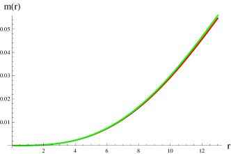
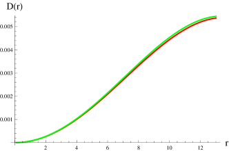
Figure 1: Plots of mass, compactness and redshift parameters corresponding to $\xi=0.2$ (red) and $\xi=0.8$ (green) for Solution-I.

As this theory involves complicated functional form, thus for our ease, we adopt a linear model [11] engaging an arbitrary constant $\varrho$ to investigate the physical feasibility of the obtained solutions as

$$f(\mathcal{R},\mathcal{T},\mathcal{R}_{\gamma\chi}\mathcal{T}^{\gamma\chi})=\mathcal{R}+\varrho\mathcal{R}_{\gamma\chi}\mathcal{T}^{\gamma\chi}.$$ (59)

We set $\varrho=-0.1$ and fix the constant $Z$ given in equation (42) to analyze Solution-I physically. Equations (31) and (32) present the values of parameters $X$ and $Y$. As the above model encompasses the contraction of Ricci tensor with the energy-momentum tensor, thus the effects of non-minimal matter-geometry interaction can still be entailed on the massive test particles. The mass of anisotropic sphere (6) is analyzed in Figure 1 (upper left) for two values of the decoupling parameter, $\xi=0.1$ and $0.9$. We find that the mass increases slowly with rise in $\xi$. Figure 1 (right and lower) displays the compactness and redshift parameters of the considered structure whose ranges are confirmed to be within their respective bounds.

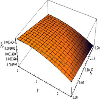
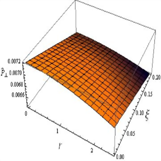
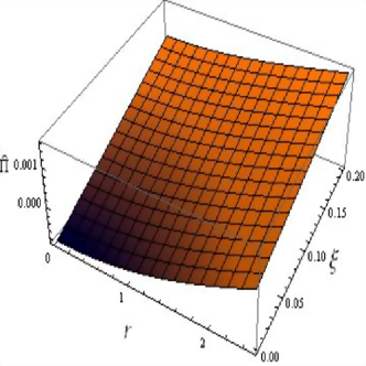
Figure 2: Plots of $\hat{\mu},~{}\hat{\mathcal{P}}_{r},~{}\hat{\mathcal{P}}_{\bot}$ and $\hat{\Pi}$ versus $r$ and $\xi$ with $\breve{M}=1M_{\bigodot}$ and $H=(0.2)^{-1}M_{\bigodot}$ for Solution-I.

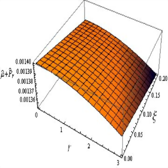
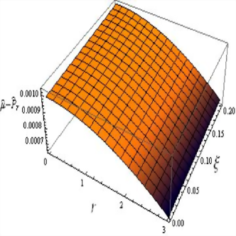
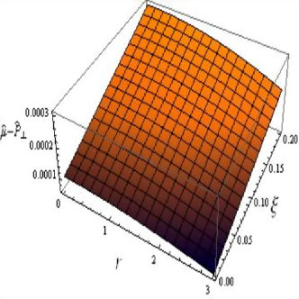
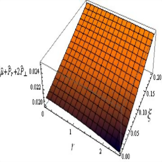
Figure 3: Plots of energy conditions versus $r$ and $\xi$ with $\breve{M}=1M_{\bigodot}$ and $H=(0.2)^{-1}M_{\bigodot}$ for Solution-I.

In the core of a celestial object, the physical variables (such as pressure and energy density) should have finite, maximum and positive values, while their behavior must decrease monotonically towards the surface of star. Figure 2 (upper left) shows that the effective energy density gains its maximum value in the middle and decreases by increasing $r$. The effective energy density enhances linearly with the increase of decoupling parameter, thus larger is the decoupling parameter, more dense is the star. Figure 2 also shows that the plots of radial and tangential pressures are similar for the parameter $\varrho$ and decrease with rise in $r$ as well as $\xi$. The anisotropic factor $\hat{\Pi}$ vanishes at the center and increases with the increase in $\xi$ which reveals that the system contains stronger anisotropy due to the decoupling parameter. By means of graphical interpretation with different values of the coupling constant $\varrho$, we examine that small negative values of $\varrho$ provide the compatible physical variables, while its positive values show their counter behavior. Figure 3 shows that all energy conditions (57) are satisfied, hence our first solution is physically viable. It is important to mention here that our Solution-I provides stable configuration throughout the system, as shown by Figure 4.

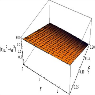
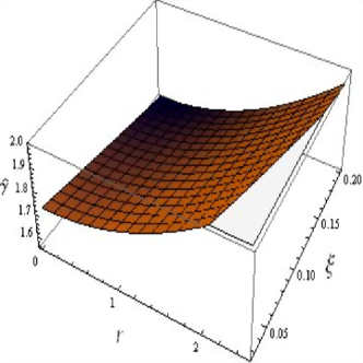
Figure 4: Plots of $|v_{s\perp}^{2}-v_{sr}^{2}|$ and adiabatic index versus $r$ and $\xi$ with $\breve{M}=1M_{\bigodot}$ and $H=(0.2)^{-1}M_{\bigodot}$ for Solution-I.

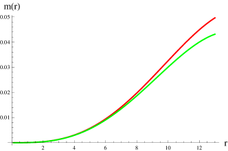
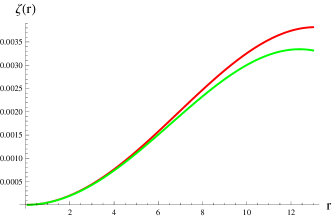
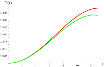
Figure 5: Plots of mass, compactness and redshift parameters corresponding to $\xi=0.10$ (red) and $\xi=0.14$ (green) for Solution-II.

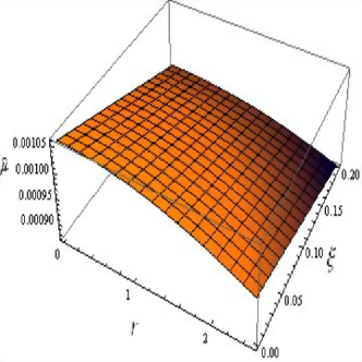
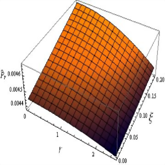
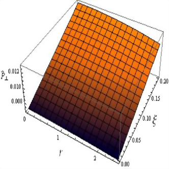
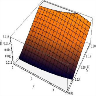
Figure 6: Plots of $\hat{\mu},~{}\hat{\mathcal{P}}_{r},~{}\hat{\mathcal{P}}_{\bot}$ and $\hat{\Pi}$ versus $r$ and $\xi$ with $\breve{M}=1M_{\bigodot}$ and $H=(0.2)^{-1}M_{\bigodot}$ for Solution-II.

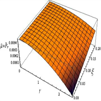
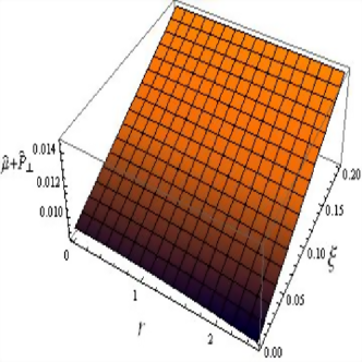
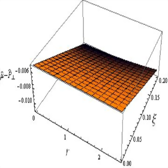
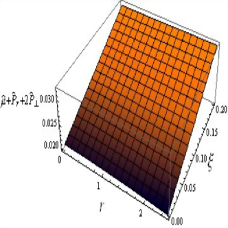
Figure 7: Plots of energy conditions versus $r$ and $\xi$ with $\breve{M}=1M_{\bigodot}$ and $H=(0.2)^{-1}M_{\bigodot}$ for Solution-II.

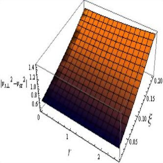
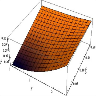
Figure 8: Plots of $|v_{s\perp}^{2}-v_{sr}^{2}|$ and adiabatic index versus $r$ and $\xi$ with $\breve{M}=1M_{\bigodot}$ and $H=(0.2)^{-1}M_{\bigodot}$ for Solution-II.

The physical features of our developed Solution-II are now being examined by taking $\varrho=-0.05$. The constants $X$ and $Z$ are shown in equations (31) and (51). Figure 5 (upper left) shows decreasing behavior of the mass of sphere (6) with increasing $\xi$. It can also be seen from the same figure (upper right and lower) that the compactness $(\zeta(r))$ and redshift $(D(r))$ comply with their required limits. The behavior of material variables and anisotropy is illustrated in Figure 6. The effective energy density decreases with rise in the decoupling parameter whereas both the effective pressures increase linearly. Figure 6 (lower right) discloses that the behavior of anisotropy is monotonically increasing with respect to $\xi$. Our second solution fulfills all energy conditions (57) except $\hat{\mu}-\hat{\mathcal{P}}_{\bot}\geq 0$, as shown in Figure 7. Hence, it is not physically viable. Figure 8 (right) confirms that the Solution-II is unstable for all values of parameter $\xi$ as it does not fulfill the required limit of adiabatic index, i.e., it takes value less than $\frac{4}{3}$ throughout.

5 Conclusions

This paper is intended to examine two different anisotropic solutions for spherically symmetric spacetime for a linear model $\mathcal{R}+\varrho\mathcal{Q}$ in $f(\mathcal{R},\mathcal{T},\mathcal{Q})$ gravity. We have utilized EGD technique to find such solutions. We have introduced an additional source $\Delta_{\gamma\chi}$ in the modified action and obtained anisotropic field equations which have further been divided into two sets by employing deformation functions. We have assumed the isotropic Krori-Barua ansatz to deal with the first set in this gravity involving three unknowns which have been calculated through junction conditions. The second sector (20)-(22) involves five unknowns, thus we have employed two constraints to close the system, one of them is the equation of state $\Delta^{0}_{0}=\alpha\Delta^{1}_{1}+\beta\Delta^{2}_{2}$ which depends upon anisotropic components. The other constraint has been taken as pressure-like or density-like which has led to the Solutions-I and II, respectively.

In order to check the feasibility of both solutions corresponding to the decoupling parameter, we have checked the graphs of effective forms of physical variables $(\hat{\mu},\hat{\mathcal{P}}_{r},\hat{\mathcal{P}}_{\bot})$, pressure anisotropy $(\hat{\Pi})$ as well as energy bounds (57) by taking $\varrho=-0.1$ and $-0.05$. The redshift and compactness for both solutions have been found to be in their respective limits. The self-gravitating geometry (6) becomes more massive for Solution-I as the decoupling parameter $\xi$ increases, while the mass decreases in case of the Solution-II. We have also explored the stability of these solutions through two approaches. The first solution provides viable as well as stable geometry, while the sphere (6) does not meet the criteria of viability and stability for Solution-II. We summarize that the behavior of these modified solutions are in contrast with GR [47, 48] and $f(\mathcal{G})$ theory [49], as Solution-I shows more stable behavior while Solution-II is not stable throughout. The resulting Solution-I is also not compatible with [38] as that solution is not stable throughout the considered range of the parameter $\xi$, i.e., $(0,0.28)$. Finally, these results can be reduced to GR by considering $f(\mathcal{R},\mathcal{T},\mathcal{Q})=\mathcal{R}$ in the action (1).

Appendix A

The modified corrections appear in equations (8)-(10) are given as

$$\mathcal{T}_{0}^{0(\mathcal{D})} = \frac{1}{f_{\mathcal{R}}+\mu f_{\mathcal{Q}}}\left[\mu\left\{f_{\mathcal{Q}}\left(\frac{\psi^{\prime 2}}{2e^{\phi}}-\frac{\psi^{\prime}}{re^{\phi}}+\frac{\psi^{\prime}\phi^{\prime}}{4e^{\phi}}-\frac{\psi^{\prime\prime}}{2e^{\phi}}-\frac{1}{2}\mathcal{R}\right)+f^{\prime}_{\mathcal{Q}}\left(\frac{\psi^{\prime}}{2e^{\phi}}\right.\right.\right.$$

$$- \left.\left.\frac{\phi^{\prime}}{4e^{\phi}}+\frac{1}{re^{\phi}}\right)+\frac{f^{\prime\prime}_{\mathcal{Q}}}{2e^{\phi}}-2f_{\mathcal{T}}\right\}+\mu^{\prime}\left\{f_{\mathcal{Q}}\left(\frac{\psi^{\prime}}{2e^{\phi}}+\frac{1}{re^{\phi}}-\frac{\phi^{\prime}}{4e^{\phi}}\right)+\frac{f^{\prime}_{\mathcal{Q}}}{e^{\phi}}\right\}$$

$$+ \frac{f_{\mathcal{Q}}\mu^{\prime\prime}}{2e^{\phi}}+\mathcal{P}\left\{f_{\mathcal{Q}}\left(\frac{3\phi^{\prime 2}}{4e^{\phi}}-\frac{2}{r^{2}e^{\phi}}-\frac{\phi^{\prime\prime}}{2e^{\phi}}\right)-f^{\prime}_{\mathcal{Q}}\left(\frac{5\phi^{\prime}}{4e^{\phi}}-\frac{1}{re^{\phi}}\right)+\frac{f^{\prime\prime}_{\mathcal{Q}}}{2e^{\phi}}\right\}$$

$$+ \mathcal{P}^{\prime}\left\{f_{\mathcal{Q}}\left(\frac{1}{re^{\phi}}-\frac{5\phi^{\prime}}{4e^{\phi}}\right)+\frac{f^{\prime}_{\mathcal{Q}}}{e^{\phi}}\right\}+\frac{f_{\mathcal{Q}}\mathcal{P}^{\prime\prime}}{2e^{\phi}}+\frac{\mathcal{R}f_{\mathcal{R}}}{2}+f^{\prime}_{\mathcal{R}}\left(\frac{\phi^{\prime}}{2e^{\phi}}-\frac{2}{re^{\phi}}\right)$$

$$- \left.\frac{f^{\prime\prime}_{\mathcal{R}}}{e^{\phi}}-\frac{f}{2}\right],$$

$$\mathcal{T}_{1}^{1(\mathcal{D})} = \frac{1}{f_{\mathcal{R}}+\mu f_{\mathcal{Q}}}\left[\mu\left(f_{\mathcal{T}}-\frac{f_{\mathcal{Q}}\psi^{\prime 2}}{4e^{\phi}}+\frac{f^{\prime}_{\mathcal{Q}}\psi^{\prime}}{4e^{\phi}}\right)+\frac{f_{\mathcal{Q}}\mu^{\prime}\psi^{\prime}}{4e^{\phi}}+\mathcal{P}\left\{f_{\mathcal{T}}+f_{\mathcal{Q}}\left(\frac{\psi^{\prime\prime}}{e^{\phi}}\right.\right.\right.$$

$$- \left.\left.\frac{\phi^{\prime 2}}{e^{\phi}}+\frac{\psi^{\prime 2}}{2e^{\phi}}-\frac{3\psi^{\prime}\phi^{\prime}}{4e^{\phi}}-\frac{3\phi^{\prime}}{re^{\phi}}+\frac{2}{r^{2}e^{\phi}}+\frac{1}{2}\mathcal{R}\right)-f^{\prime}_{\mathcal{Q}}\left(\frac{\psi^{\prime}}{4e^{\phi}}+\frac{2}{re^{\phi}}\right)\right\}$$

$$- \left.\mathcal{P}^{\prime}f_{\mathcal{Q}}\left(\frac{\psi^{\prime}}{4e^{\phi}}+\frac{2}{re^{\phi}}\right)+\frac{f}{2}-\frac{\mathcal{R}f_{\mathcal{R}}}{2}-f^{\prime}_{\mathcal{R}}\left(\frac{\psi^{\prime}}{2e^{\phi}}+\frac{2}{re^{\phi}}\right)\right],$$

$$\mathcal{T}_{2}^{2(\mathcal{D})} = \frac{1}{f_{\mathcal{R}}+\mu f_{\mathcal{Q}}}\left[\mu\left(f_{\mathcal{T}}-\frac{f_{\mathcal{Q}}\psi^{\prime 2}}{4e^{\phi}}+\frac{f^{\prime}_{\mathcal{Q}}\psi^{\prime}}{4e^{\phi}}\right)+\frac{f_{\mathcal{Q}}\mu^{\prime}\psi^{\prime}}{4e^{\phi}}+\mathcal{P}\left\{f_{\mathcal{T}}+f_{\mathcal{Q}}\left(\frac{\phi^{\prime\prime}}{2e^{\phi}}\right.\right.\right.$$

$$+ \left.\frac{\psi^{\prime}}{2re^{\phi}}-\frac{3\phi^{\prime 2}}{4e^{\phi}}-\frac{\phi^{\prime}}{2re^{\phi}}+\frac{1}{r^{2}e^{\phi}}-\frac{2}{r^{2}}+\frac{1}{2}\mathcal{R}\right)+f^{\prime}_{\mathcal{Q}}\left(\frac{3\phi^{\prime}}{2e^{\phi}}-\frac{\psi^{\prime}}{4e^{\phi}}-\frac{3}{re^{\phi}}\right)$$

$$- \left.\frac{f^{\prime\prime}_{\mathcal{Q}}}{e^{\phi}}\right\}+\mathcal{P}^{\prime}\left\{f_{\mathcal{Q}}\left(\frac{3\phi^{\prime}}{2e^{\phi}}-\frac{\psi^{\prime}}{4e^{\phi}}-\frac{3}{re^{\phi}}\right)-\frac{2f^{\prime}_{\mathcal{Q}}}{e^{\phi}}\right\}-\frac{f_{\mathcal{Q}}\mathcal{P}^{\prime\prime}}{e^{\phi}}-\frac{\mathcal{R}f_{\mathcal{R}}}{2}+\frac{f}{2}$$

$$+ \left.f^{\prime}_{\mathcal{R}}\left(\frac{\phi^{\prime}}{2e^{\phi}}-\frac{\psi^{\prime}}{2e^{\phi}}-\frac{1}{re^{\phi}}\right)-\frac{f^{\prime\prime}_{\mathcal{R}}}{e^{\phi}}\right].$$

The quantity $\Omega$ in equation (12) turns out to be

$$\Omega =\frac{2}{\left(\mathcal{R}f_{\mathcal{Q}}+2(1+f_{\mathcal{T}})\right)}\left[f^{\prime}_{\mathcal{Q}}e^{-\phi}\mathcal{P}\left(\frac{1}{r^{2}}-\frac{e^{\phi}}{r^{2}}+\frac{\psi^{\prime}}{r}\right)+f_{\mathcal{Q}}e^{-\phi}\mathcal{P}\left(\frac{\psi^{\prime\prime}}{r}-\frac{\psi^{\prime}}{r^{2}}-\frac{\phi^{\prime}}{r^{2}}\right.\right.$$

$$-\left.\frac{\psi^{\prime}\phi^{\prime}}{r}-\frac{2}{r^{3}}+\frac{2e^{\phi}}{r^{3}}\right)+\mathcal{P}^{\prime}\left\{f_{\mathcal{Q}}e^{-\phi}\left(\frac{\psi^{\prime}\phi^{\prime}}{8}-\frac{\psi^{\prime\prime}}{8}-\frac{\psi^{\prime 2}}{8}+\frac{\phi^{\prime}}{2r}+\frac{\psi^{\prime}}{2r}+\frac{1}{r^{2}}-\frac{e^{\phi}}{r^{2}}\right)\right.$$

$$+\left.\frac{3}{4}f_{\mathcal{T}}\right\}+\mathcal{P}f^{\prime}_{\mathcal{T}}-\mu f^{\prime}_{\mathcal{T}}-\mu^{\prime}\left\{\frac{f_{\mathcal{Q}}e^{-\phi}}{8}\left(\psi^{\prime 2}-\psi^{\prime}\phi^{\prime}+2\psi^{\prime\prime}+\frac{4\psi^{\prime}}{r}\right)+\frac{3f_{\mathcal{T}}}{2}\right\}$$

$$-\left.\left(\frac{e^{-\phi}}{r^{2}}-\frac{1}{r^{2}}+\frac{\psi^{\prime}e^{-\phi}}{r}\right)\left(\mu^{\prime}f_{\mathcal{Q}}+\mu f^{\prime}_{\mathcal{Q}}\right)\right].$$

References

- [1] Nojiri, S. and Odintsov, S.D.: Phys. Rev. D 68(2003)123512.
- [2] Cognola, G., et al.: J. Cosmol. Astropart. Phys. 02(2005)010.
- [3] Song, Y.S., Hu, W. and Sawicki, I.: Phys. Rev. D 75(2007)044004.
- [4] Capozziello, S. et al.: Phys. Rev. D 83(2011)064004.
- [5] Sharif, M. and Kausar, H.R.: J. Cosmol. Astropart. Phys. 07(2011)022.
- [6] Arapoğlu, S., Deliduman, C. and Ekşi, K.Y.: J. Cosmol. Astropart. Phys. 07(2011)020.
- [7] Sharif, M. and Yousaf, Z.: Astropart. Phys. 56(2014)19.
- [8] Astashenok, A.V., Capozziello, S. and Odintsov, S.D.: Phys. Rev. D 89(2014)103509.
- [9] Bertolami, O. et al.: Phys. Rev. D 75(2007)104016.
- [10] Harko, T. et al.: Phys. Rev. D 84(2011)024020.
- [11] Haghani, Z. et al.: Phys. Rev. D 88(2013)044023.
- [12] Sharif, M. and Zubair, M.: J. Cosmol. Astropart. Phys. 11(2013)042.
- [13] Sharif, M. and Zubair, M.: J. High Energy Phys. 12(2013)079.
- [14] Odintsov, S.D. and Sáez-Gómez, D.: Phys. Lett. B 725(2013)437.
- [15] Ayuso, I., Jiménez, J.B. and De la Cruz-Dombriz, A.: Phys. Rev. D 91(2015)104003.
- [16] Baffou, E.H., Houndjo, M.J.S. and Tosssa, J.: Astrophys. Space Sci. 361(2016)376.
- [17] Yousaf, Z., Bhatti, M.Z. and Naseer, T.: Eur. Phys. J. Plus 135(2020)353.
- [18] Yousaf, Z., Bhatti, M.Z. and Naseer, T.: Phys. Dark Universe 28(2020)100535.
- [19] Yousaf, Z., Bhatti, M.Z. and Naseer, T.: Int. J. Mod. Phys. D 29(2020)2050061.
- [20] Yousaf, Z., Bhatti, M.Z. and Naseer, T.: Ann. Phys. 420(2020)168267.
- [21] Yousaf, Z. et al.: Phys. Dark Universe 29(2020)100581.
- [22] Yousaf, Z. et al.: Mon. Not. R. Astron. Soc. 495(2020)4334.
- [23] M. Sharif, T. Naseer, Chin. J. Phys. 73 (2021) 179.
- [24] T. Naseer, M. Sharif, Universe 8 (2022) 62.
- [25] M. Sharif, T. Naseer, Phys. Scr. 97 (2022) 055004.
- [26] M. Sharif, T. Naseer, arXiv:2203.03268v1 [gr-qc] (2022).
- [27] Sharif, M. and Waseem, A.: Eur. Phys. J. Plus 131(2016)190.
- [28] Sharif, M. and Waseem, A.: Can. J. Phys. 94(2016)1024.
- [29] Maurya, S.K. et al.: Phys. Rev. D 100(2019)044014.
- [30] Shamir, M.F. and Fayyaz, I.: Theor. Math. Phys. 202(2020)112.
- [31] Ovalle, J.: Mod. Phys. Lett. A 23(2008)3247.
- [32] Ovalle, J. and Linares, F.: Phys. Rev. D 88(2013)104026.
- [33] Casadio, R., Ovalle, J. and Da Rocha, R.: Class. Quantum Grav. 32(2015)215020.
- [34] Ovalle, J.: Phys. Rev. D 95(2017)104019.
- [35] Ovalle, J., et al.: Eur. Phys. J. C 78(2018)960.
- [36] Gabbanelli, L., Rincón, Á. and Rubio, C.: Eur. Phys. J. C 78(2018)370.
- [37] Estrada, M. and Tello-Ortiz, F.: Eur. Phys. J. Plus 133(2018)453.
- [38] Sharif, M. and Sadiq, S.: Eur. Phys. J. C 78(2018)410.
- [39] Sharif, M. and Saba, S.: Eur. Phys. J. C 78(2018)921.
- [40] Sharif, M. and Saba, S.: Chin. J. Phys. 59(2019)481.
- [41] Sharif, M. and Waseem, A.: Ann. Phys. 405(2019)14.
- [42] Sharif, M. and Waseem, A.: Chin. J. Phys. 60(2019)426.
- [43] Singh, K.N. et al.: Eur. Phys. J. C 79(2019)851.
- [44] Hensh, S. and Stuchlík, Z.: Eur. Phys. J. C 79(2019)834.
- [45] Ovalle, J.: Phys. Lett. B 788(2019)213.
- [46] Contreras, E. and Bargueño, P.: Class. Quantum Grav. 36(2019)215009.
- [47] Sharif, M. and Ama-Tul-Mughani, Q.: Ann. Phys. 415(2020)168122.
- [48] Sharif, M. and Ama-Tul-Mughani, Q.: Chin. J. Phys. 65(2020)207.
- [49] Sharif, M. and Saba, S.: Int. J. Mod. Phys. D 29(2020)2050041.
- [50] Sharif, M. and Majid, A.: Chin. J. Phys. 68(2020)406.
- [51] Sharif, M. and Majid, A.: Phys. Dark Universe 30(2020)100610.
- [52] Sharif, M. and Majid, A.: Phys. Scr. 96(2021)035002.
- [53] Krori, K.D. and Barua, J.: J. Phys. A: Math. Gen. 8(1975)508.
- [54] Buchdahl, H.A.: Phys. Rev. D 116(1959)1027.
- [55] Ivanov, B.V.: Phys. Rev. D 65(2002)104011.
- [56] Heintzmann, H. and Hillebrandt, W.: Astron. Astrophys. 38(1975)51.