Monge, Bregman and Occam: Interpretable Optimal Transport in High-Dimensions with Feature-Sparse Maps

Abstract

Optimal transport (OT) theory focuses, among all maps $T:\mathbb{R}^{d}\rightarrow\mathbb{R}^{d}$ that can morph a probability measure onto another, on those that are the “thriftiest”, i.e. such that the averaged cost $c(\mathbf{x},T(\mathbf{x}))$ between $\mathbf{x}$ and its image $T(\mathbf{x})$ be as small as possible. Many computational approaches have been proposed to estimate such Monge maps when $c$ is the $\ell_{2}^{2}$ distance, e.g., using entropic maps (Pooladian and Niles-Weed, 2021), or neural networks (Makkuva et al., 2020; Korotin et al., 2020). We propose a new model for transport maps, built on a family of translation invariant costs $c(\mathbf{x},\mathbf{y}):=h(\mathbf{x}-\mathbf{y})$, where $h:=\tfrac{1}{2}\|\cdot\|_{2}^{2}+\tau$ and $\tau$ is a regularizer. We propose a generalization of the entropic map suitable for $h$, and highlight a surprising link tying it with the Bregman centroids of the divergence $D_{h}$ generated by $h$, and the proximal operator of $\tau$. We show that choosing a sparsity-inducing norm for $\tau$ results in maps that apply Occam’s razor to transport, in the sense that the displacement vectors $\Delta(\mathbf{x}):=T(\mathbf{x})-\mathbf{x}$ they induce are sparse, with a sparsity pattern that varies depending on $\mathbf{x}$. We showcase the ability of our method to estimate meaningful OT maps for high-dimensional single-cell transcription data, in the $34000$-$d$ space of gene counts for cells, without using dimensionality reduction, thus retaining the ability to interpret all displacements at the gene level.

1 Introduction

A fundamental task in machine learning is learning how to transfer observations from a source to a target probability measure. For such problems, optimal transport (OT) (Santambrogio, 2015) has emerged as a powerful toolbox that can improve performance and guide theory in various settings. For instance, the computational approaches advocated in OT have been used to transfer knowledge across datasets in domain adaptation tasks (Courty et al., 2016, 2017), train generative models (Montavon et al., 2016; Arjovsky et al., 2017; Genevay et al., 2018; Salimans et al., 2018), and realign datasets in natural sciences (Janati et al., 2019; Schiebinger et al., 2019).

High-dimensional Transport. OT finds its most straightforward and intuitive use-cases in low-dimensional geometric domains (grids and meshes, graphs, etc…). This work focuses on the more challenging problem of using it on distributions in $\mathbb{R}^{d}$, with $d\gg 1$. In $\mathbb{R}^{d}$, the ground cost $c(\mathbf{x},\mathbf{y})$ between observations $\mathbf{x},\mathbf{y}$ is often the $\ell_{2}$ metric or its square $\ell_{2}^{2}$. However, when used on large-$d$ data samples, that choice is rarely meaningful. This is due to the curse-of-dimensionality associated with OT estimation (Dudley et al., 1966; Weed and Bach, 2019) and the fact that the Euclidean distance loses its discriminative power as dimension grows. To mitigate this, practitioners rely on dimensionality reduction, either in two steps, before running OT solvers, using, e.g., PCA, a VAE, or a sliced-Wasserstein approach (Rabin et al., 2012; Bonneel et al., 2015); or jointly, by estimating both a projection and transport, e.g., on hyperplanes (Niles-Weed and Rigollet, 2022; Paty and Cuturi, 2019; Lin et al., 2020; Huang et al., 2021; Lin et al., 2021), lines (Deshpande et al., 2019; Kolouri et al., 2019), trees (Le et al., 2019) or more advanced featurizers (Salimans et al., 2018). However, an obvious drawback of these approaches is that transport maps estimated in reduced dimensions are hard to interpret in the original space (Muzellec and Cuturi, 2019).

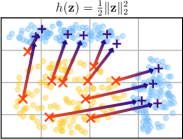
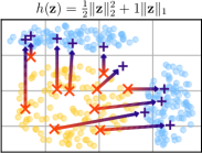
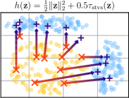
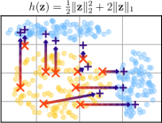
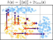
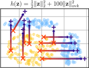
Figure 1: Plots of entropic map estimators $T_{h,\varepsilon}$, as defined in Prop. 4.2, to map a 2D measure supported on $(\mathbf{x}^{i})$ onto that supported on $(\mathbf{y}^{j})$, for various costs $h$. The displacements $\Delta(\mathbf{x})=T_{h,\varepsilon}(\mathbf{x})-\mathbf{x}$ of unseen points are displayed as arrows. From left to right: standard $\ell_{2}^{2}$ norm, Elastic $\ell_{1}$, STVS, and $k$-support costs ($k=1$). For each proposed cost, the regularization $\gamma$ is small on the top row and high on the bottom. Displacements are not sparse for the $\ell_{2}^{2}$ cost but become increasingly so as $\gamma$ grows, with a support that varies with input $\mathbf{x}$. Note that Elastic $\ell_{1}$ and STVS tend to censor displacements as $\gamma$ grows, to the extent that they become null. In contrast, the $k$-support cost encourages sparsity but enforces displacements with at least $k$ non-zero values. See also Figure 2 for aggregate results.

Contributions. To target high $d$ regimes, we introduce a radically different approach. We use the sparsity toolbox (Hastie et al., 2015; Bach et al., 2012) to build OT maps that are, adaptively to input $\mathbf{x}$, drastically simpler:

• We introduce a generalized entropic map (Pooladian and Niles-Weed, 2021) for translation invariant costs $c(\mathbf{x},\mathbf{y}):=h(\mathbf{x}-\mathbf{y})$, where $h$ is strongly convex. That entropic map $T_{h,\varepsilon}$ is defined almost everywhere (a.e.), and we show that it induces displacements $\Delta(\mathbf{x}):=T(\mathbf{x})-\mathbf{x}$ that can be cast as Bregman centroids, relative to the Bregman divergence generated by $h$.

• When $h$ is an elastic-type regularizer, the sum of a strongly-convex term $\ell_{2}^{2}$ and a sparsifying norm $\tau$, we show that such centroids are obtained using the proximal operator of $\tau$. This induces sparse displacements $\Delta(\mathbf{x})$, with a sparsity pattern that depends on $\mathbf{x}$, controlled by the regularization strength set for $\tau$. To our knowledge, our formulation is the first in the computational OT literature that can produce features-wise sparse OT maps.

• We apply our method to single-cell transcription data using two different sparsity-inducing proximal operators. We show that this approach succeeds in recovering meaningful maps in extremely high-dimension.

Not the Usual Sparsity found in Computational OT. Let us emphasize that the sparsity studied in this work is unrelated, and, in fact, orthogonal, to the many references to sparsity found in the computational OT literature. Such references arise when computing an OT plan from $n$ to $m$ points, resulting in large $n\times m$ optimal coupling matrices. Such matrices are sparse when any point in the source measure is only associated to one or a few points in the target measure. Such sparsity acts at the level of samples, and is usually a direct consequence of linear programming duality (Peyré and Cuturi, 2019, Proposition 3.4). It can be also encouraged with regularization (Courty et al., 2016; Dessein et al., 2018; Blondel et al., 2018) or constraints (Liu et al., 2022). By contrast, sparsity in this work only occurs relative to the features of the displacement vector $\Delta(\mathbf{x})\in\mathbb{R}^{d}$, when moving a given $\mathbf{x}$, i.e., $\|\Delta(\mathbf{x})\|_{0}\ll d$. Note, finally, that we do not use coupling matrices in this paper.

Links to OT Theory with Degenerate Costs. Starting with the seminal work by Sudakov (1979), who proved the existence of Monge maps for the original Monge problem, studying non-strongly convex costs with gradient discontinuities (Santambrogio, 2015, §3) has been behind many key theoretical developments (Ambrosio and Pratelli, 2003; Ambrosio et al., 2004; Evans and Gangbo, 1999; Trudinger and Wang, 2001; Carlier et al., 2010; Bianchini and Bardelloni, 2014). While these works have few practical implications, because they focus on the existence of Monge maps, constructed by stitching together OT maps defined pointwise, they did, however, guide our work in the sense that they shed light on the difficulties that arise from “flat” norms such as $\ell_{1}$. This has guided our focus in this work on elastic-type norms, which allow controlling the amount of sparsity through regularization strength, by analogy with the Lasso tradeoff where an $\ell_{2}^{2}$ loss is paired with an $\ell_{1}$ regularizer.

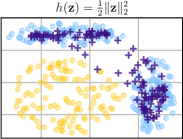
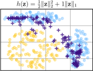
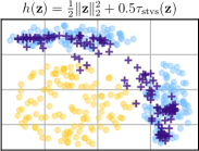
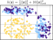
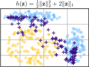
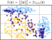
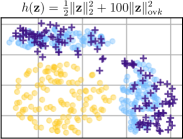
Figure 2: Follow-up to Figure 1, where a fresh sample of points from the base measure is transported using the various entropic map estimators $T_{h,\varepsilon}$ that were considered. Paired with Figure 1, this plot shows the tradeoff, controlled by $\gamma$, between the sparsity of displacements and the ability to recover the target measure (as $\gamma$ increases, ultimately, the map no longer moves points.). An interesting feature of the $\|\cdot\|_{\mathrm{ov}k}$ norm resides in its ability, no matter what $\gamma$, to enforce at least one displacement (here $k=1$).

2 Background

2.1 The Monge Problem.

Consider a translation-invariant cost function $c(\mathbf{x},\mathbf{y}):=h(\mathbf{x}-\mathbf{y})$, where $h:\mathbb{R}^{d}\rightarrow\mathbb{R}$. The Monge problem (1781) consists of finding, among all maps $T:\mathbb{R}^{d}\rightarrow\mathbb{R}^{d}$ that push-forward a measure $\mu\in\mathcal{P}(\mathbb{R}^{d})$ onto $\nu\in\mathcal{P}(\mathbb{R}^{d})$, the map which minimizes the average length (as measured by $h$) of its displacements:

$$T^{\star}:=\operatorname*{arg\,inf}_{T\sharp\mu=\nu}\int_{\mathbb{R}^{d}}h(\mathbf{x}-T(\mathbf{x}))\,\mathrm{d}\mu\,.$$ (1)

From Dual Potentials to Optimal Maps.

Problem (1) is notoriously difficult to solve directly since the set of admissible maps $T$ is not even convex. The defining feature of OT theory to obtain an optimal push-forward solution $T^{\star}$ is to cast Problem (1) as a linear optimization problem: relax the requirement that $\mathbf{x}$ is mapped onto a single point $T(\mathbf{x})$, to optimize instead over the space of couplings of $\mu,\nu$, namely on the set $\Pi(\mu,\nu)$ of probability distributions in $\mathcal{P}(\mathbb{R}^{d}\times\mathbb{R}^{d})$ with marginals $\mu,\nu$:

$$P^{\star}:=\operatorname*{arg\,inf}_{P\in\Pi(\mu,\nu)}\iint_{\mathbb{R}^{d}\times\mathbb{R}^{d}}c\,\mathrm{d}P\,.$$ (2)

If $T^{\star}$ is optimal for  Equation 1, then $(\text{Id},T^{\star})\sharp\mu$ is trivially an optimal coupling. To recover a map $T^{\star}$ from a coupling $P^{\star}$ requires considering the dual to (2):

$$f^{\star},g^{\star}\in\operatorname*{arg\,sup}_{\begin{subarray}{c}f,g:\mathbb{R}^{d}\rightarrow\mathbb{R}\\ f\oplus g\leq c\end{subarray}}\,\,\int_{\mathbb{R}^{d}}f\,\mathrm{d}\mu+\int_{\mathbb{R}^{d}}g\,\mathrm{d}\nu\,,$$ (3)

where $\forall\,\mathbf{x},\mathbf{y}$ we write $(f\oplus g)(\mathbf{x},\mathbf{y}):=f(\mathbf{x})+g(\mathbf{y})$.

Leaving aside how such couplings and dual potentials can be approximated from data (this will be discussed in the next section), suppose that we have access to an optimal dual pair $(f^{\star},g^{\star})$. By a standard duality argument (Santambrogio, 2015, §1.3), if a pair $(\mathbf{x}^{0},\mathbf{y}^{0})$ lies in the support of $P^{\star}$, $\operatorname{supp}(P^{\star})$, the constraint for dual variables is saturated, i.e.,

$$f^{\star}(\mathbf{x}^{0})+g^{\star}(\mathbf{y}^{0})=h(\mathbf{x}^{0}-\mathbf{y}^{0})\,,$$

Additionally, by a so-called $c$-concavity argument one has:

$$g^{\star}(\mathbf{y}^{0})=\inf_{\mathbf{x}}h(\mathbf{x}-\mathbf{y}^{0})-f^{\star}(\mathbf{x}).\,$$

Assuming $f^{\star}$ is differentiable at $\mathbf{x}^{0}$, combining these two results yields perhaps the most pivotal result in OT theory:

$$(\mathbf{x}^{0},\mathbf{y}^{0})\in\operatorname{supp}(P^{\star})\Leftrightarrow\nabla f^{\star}(\mathbf{x}^{0})\in\partial h(\mathbf{x}^{0}-\mathbf{y}^{0})\,,$$ (4)

where $\partial h$ denotes the subdifferential of $h$, see, e.g. (Carlier et al., 2010). Let $h^{*}$ be the convex conjugate of $h$,

$$h^{*}(\mathbf{y}):=\sup_{x\in\mathbb{R}^{d}}\langle\mathbf{x},\mathbf{y}\rangle-h(\mathbf{x}).$$

Depending on $h$, two cases arise in the literature:

• If $h$ is differentiable everywhere, strictly convex, one has:

  $$\nabla f^{\star}(\mathbf{x}^{0})=\nabla h(\mathbf{x}^{0}-\mathbf{y}^{0})\,.$$

  Thanks to the identity $\nabla h^{*}=(\nabla h)^{-1}$, one can uniquely characterize the only point $\mathbf{y}^{0}$ to which $\mathbf{x}^{0}$ is associated in the optimal coupling $P^{\star}$ as $\mathbf{x}^{0}-\nabla h^{*}(\nabla f^{\star}(\mathbf{x}^{0}))$. More generally one recovers therefore for any $\mathbf{x}$ in $\operatorname{supp}(\mu)$:

  $$T^{\star}(\mathbf{x})=\mathbf{x}-\nabla h^{*}\circ\nabla f^{\star}(\mathbf{x})\,.$$ (5)

  The Brenier theorem (1991) is a particular case of that result, which states that when $h=\frac{1}{2}\|\cdot\|^{2}_{2}$, we have $T(\mathbf{x})=\mathbf{x}-\nabla f^{\star}(\mathbf{x}^{0})$, since in that case $\nabla h=\nabla h^{*}=(\nabla h)^{-1}=\text{Id}$, see (Santambrogio, 2015, Theo. 1.22).

• If $h$ is “only” convex, then one recovers the sub-differential inclusion $\mathbf{y}^{0}\in\mathbf{x}^{0}+\partial h^{*}(\nabla f^{\star}(\mathbf{x}^{0}))$ (Ambrosio et al., 2004)(Santambrogio, 2015, §3).

In summary, given an optimal dual solution $f^{\star}$ to Problem (3), one can use differential (or sub-differential) calculus to define an optimal transport map, in the sense that it defines (uniquely or as a multi-valued map) where the mass of a point $\mathbf{x}$ should land.

2.2 Bregman Centroids

We suppose in this section that $h$ is strongly convex, in which case its convex conjugate is differentiable everywhere and gradient smooth. The generalized Bregman divergence (or B-function) generated by $h$ (Telgarsky and Dasgupta, 2012; Kiwiel, 1997) is,

$$D_{h}(\mathbf{x}|\mathbf{y})=h(\mathbf{x})-h(\mathbf{y})-\sup_{\mathbf{w}\in\partial h(\mathbf{y})}\langle\mathbf{w},\mathbf{x}-\mathbf{y}\rangle.$$

Consider a family of $k$ points $\mathbf{z}^{1},\dots,\mathbf{z}^{m}\in\mathbb{R}^{d}$ with weights $p^{1},\dots,p^{m}>0$ summing to $1$. A point in the set

$$\operatorname*{arg\,min}_{\mathbf{z}\in\mathbb{R}^{d}}\sum_{j}p^{\,j}D_{h}(\mathbf{z},\mathbf{z}^{j})\,,$$

is called a Bregman centroid (Nielsen and Nock, 2009, Theo. 3.2). Assuming $h$ is differentiable at each $\mathbf{z}^{j}$, one has that this point is uniquely defined as:

$$\mathcal{C}_{h}\left((\mathbf{z}^{j})_{j},(p^{\,j})_{i}\right):=\nabla h^{\star}\left(\sum_{j=1}^{m}p^{\,j}\nabla h(\mathbf{z}^{i})\right)\,.$$ (6)

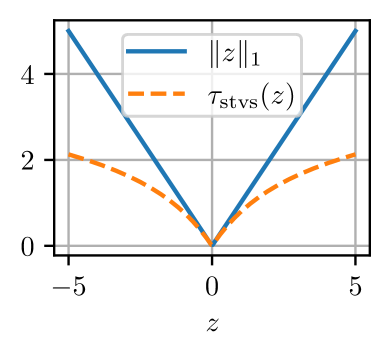
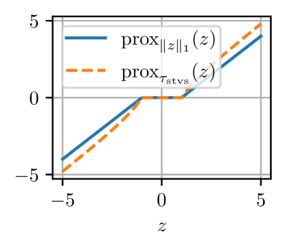
Figure 3: The STVS regularizer is not convex, but its proximal operator is well-defined and tends to shrink values less than the usual soft-thresholding operator. For instance, its values near $\{-5,5\}$ are close to the identity line.

2.3 Sparsity-Inducing Penalties

To form relevant functions $h$, we will exploit the following sparsity-inducing functions: the $\ell_{1}$ and $\|\cdot\|_{\mathrm{ov}k}$ norms, and a handcrafted penalty that mimics the thresholding properties of $\ell_{1}$ but with less shrinkage.

• For a vector $\mathbf{z}\in\mathbb{R}^{d}$, $\|\mathbf{z}\|_{p}:=(\sum_{i=1}^{d}|\mathbf{z}_{i}|^{p})^{1/p}$. We write $\ell_{2}$ and $\ell_{2}^{2}$ for $\|\cdot\|_{2}$ and $\|\cdot\|_{2}^{2}$ respectively.

• We write $\ell_{1}$ for $\|\cdot\|_{1}$. Its proximal operator $\mathrm{prox}_{\gamma\ell_{1}}(\mathbf{z})=\mathrm{ST}_{\gamma}(\mathbf{z})=(1-\gamma/|\mathbf{z}|)_{+}\odot\mathbf{z}$ is called the soft-thresholding operator.

• Schreck et al. (2015) propose the soft-thresholding operator with vanishing shrinkage (STVS),

  $$\tau_{\mathrm{stvs}}(\mathbf{z})=\gamma^{2}\mathbf{1}_{d}^{T}\left(\sigma(\mathbf{z})+\tfrac{1}{2}-\tfrac{1}{2}e^{-2\sigma(\mathbf{z})}\right)\geq 0\,,$$ (7)

  with $\sigma(\mathbf{z}):=\operatorname{asinh}\left(\frac{\mathbf{z}}{2\gamma}\right)$, and where all operations are element-wise. $\tau_{\mathrm{stvs}}$ is a non-convex regularizer, non-negative thanks to (our) addition of $+\tfrac{1}{2}$, to recover a nonnegative quantity that cancels if and only if $\mathbf{z}=0$. Schreck et al. show that the proximity operator $\operatorname{prox}_{\tau_{\mathrm{stvs}}}$, written $\mathrm{STVS}$ for short, decreases the shrinkage (see  Figure 3) observed with soft-thresholding:

  $$\mathrm{STVS}_{\gamma}(\mathbf{z})=\left(1-\gamma^{2}/|\mathbf{z}|^{2}\right)_{+}\odot\mathbf{z}\,.$$ (8)

  The Hessian of $\tau_{\mathrm{stvs}}$ is a diagonal matrix with values $\tfrac{1}{2}|\mathbf{z}|/\sqrt{\mathbf{z}^{2}+\gamma^{2}}-\tfrac{1}{2}$ and is therefore lower-bounded (with positive-definite order) by $-\tfrac{1}{2}I_{d}$.

• Let $\mathcal{G}_{k}$ be the set of all subsets of size $k$ within $\{1,\dots,d\}$. Argyriou et al. (2012) introduces the $k$-overlap norm:

  $$\|\mathbf{z}\|_{\mathrm{ov}k}=\min\{\!\sum_{I\in\mathcal{G}_{k}}\|\mathbf{v}_{I}\|_{2}\,|\,\text{supp}(\mathbf{v}_{I})\subset I,\sum_{I\in\mathcal{G}_{k}}\mathbf{v}_{I}=\mathbf{z}\}\,.$$

  For any vector $\mathbf{z}$ in $\mathbb{R}^{d}$, we write $\mathbf{z}^{\downarrow}$ for the vector composed with all entries of $\mathbf{z}$ sorted in a decreasing order. This formula can be evaluated as follows to exhibit a $\ell_{1}/\ell_{2}$ norm split between the $d$ variables in a vector:

  $$\|\mathbf{z}\|_{\mathrm{ov}k}^{2}=\sum_{i=1}^{k-r-1}(|\mathbf{z}|^{\downarrow}_{i})^{2}+\left(\sum_{i=k-r}^{d}|\mathbf{z}|^{\downarrow}_{i}\right)^{2}/(r+1)$$

  where $r\leq k-1$ is the unique integer such that

  $$|\mathbf{z}|_{k-r}^{\downarrow}\leq\sum_{i=k-r}^{d}|\mathbf{z}|^{\downarrow}_{i}<|\mathbf{z}|_{k-r-1}^{\downarrow}.$$

  Its proximal operator is too complex to be recalled here but given in (Argyriou et al., 2012, Algo. 1), running in $O(d(\log d+k))$ operations.

Note that both $\ell_{1}$ and $\tau_{\mathrm{stvs}}$ are separable—their proximal operators act element-wise—but it is not the case of $\|\cdot\|_{\mathrm{ov}k}$.

3 Generalized Entropic-Bregman Maps

Generalized Entropic Potential. When $h$ is the $\ell_{2}^{2}$ cost, and when $\mu$ and $\nu$ can be accessed through samples, i.e., $\hat{\mu}_{n}=\tfrac{1}{n}\sum_{i}\delta_{\mathbf{x}^{i}},\hat{\nu}_{m}=\tfrac{1}{m}\sum_{j}\delta_{\mathbf{y}^{j}}$, a convenient estimator for $f^{\star}$ and subsequently $T^{\star}$ is the entropic map (Pooladian and Niles-Weed, 2021; Rigollet and Stromme, 2022). We generalize these estimators for arbitrary costs $h$. Similar to the original approach, our construction starts by solving a dual entropy-regularized OT problem. Let $\varepsilon>0$ and write $K_{ij}=[\exp(-h(\mathbf{x}^{i}-\mathbf{y}^{j})/\varepsilon)]_{ij}$ the kernel matrix induced by cost $h$. Define (up to a constant):

$$\!\!\!\mathbf{f}^{\star},\mathbf{g}^{\star}=\operatorname*{arg\,max}_{\mathbf{f}\in\mathbb{R}^{n},\mathbf{g}\in\mathbb{R}^{m}}\langle\mathbf{f},\tfrac{\mathbf{1}_{n}}{n}\rangle+\langle\mathbf{g},\tfrac{\mathbf{1}_{m}}{m}\rangle-\varepsilon\langle e^{\frac{\mathbf{f}}{\varepsilon}},Ke^{\frac{\mathbf{g}}{\varepsilon}}\rangle\,.$$ (9)

Problem (9) is the regularized OT problem in dual form (Peyré and Cuturi, 2019, Prop. 4.4), an unconstrained concave optimization problem that can be solved with the Sinkhorn algorithm (Cuturi, 2013). Once such optimal vectors are computed, estimators $f_{\varepsilon},g_{\varepsilon}$ of the optimal dual functions $f^{\star},g^{\star}$ of Equation 3 can be recovered by extending these discrete solutions to unseen points $\mathbf{x},\mathbf{y}$,

$$f_{\varepsilon}(\mathbf{x})=\operatorname{min}_{\varepsilon}([h(\mathbf{x}-\mathbf{y}^{j})-\mathbf{g}^{\star}_{j}]_{j})\,,$$ (10)

$$g_{\varepsilon}(\mathbf{y})=\operatorname{min}_{\varepsilon}([h(\mathbf{x}^{i}-\mathbf{y})-\mathbf{f}^{\star}_{i}]_{i})\,,$$ (11)

where for a vector $\mathbf{u}$ or arbitrary size $s$ we define the log-sum-exp operator as $\operatorname{min}_{\varepsilon}(\mathbf{u}):=-\varepsilon\log(\tfrac{1}{s}\mathbf{1}_{s}^{T}e^{-\mathbf{u}/\varepsilon})$.

Generalized Entropic Maps.

Using the blueprint given in Equation 4, we use the gradient of these dual potential estimates to formulate maps. Such maps are only properly defined on a subset of $\mathbb{R}^{d}$ defined as follows:

$$\Omega_{\hat{\nu}_{m}}(h):=\{\mathbf{x}\,|\,\forall j\leq m,\nabla h(\mathbf{x}-\mathbf{y}^{j})\text{ exists.}\}\subset\mathbb{R}^{d}.$$ (12)

However, because a convex function is a.e. differentiable, $\Omega_{\hat{\nu}_{m}}(h)$ has measure 1 in $\mathbb{R}^{d}$. With this, $\nabla f_{\varepsilon}$ is properly defined for $\mathbf{x}$ in $\Omega_{\hat{\nu}_{m}}(h)$, as:

$$\nabla f_{\varepsilon}(\mathbf{x})=\sum_{j=1}^{m}p^{\,j}(\mathbf{x})\nabla h(\mathbf{x}-\mathbf{y}^{j})\,,$$ (13)

using the $\mathbf{x}$-varying Gibbs distribution in the $m$-simplex:

$$p^{\,j}(\mathbf{x}):=\frac{\exp\left(-\left(h(\mathbf{x}-\mathbf{y}^{j})-\mathbf{g}_{j}^{\star}\right)/\varepsilon\right)}{\sum_{k=1}^{m}\exp\left(-\left(h(\mathbf{x}-\mathbf{y}^{k})-\mathbf{g}_{k}^{\star}\right)/\varepsilon\right)}\,.$$ (14)

One can check that if $h=\tfrac{1}{2}\ell^{2}_{2}$, Equation 13 simplifies to the usual estimator (Pooladian and Niles-Weed, 2021):

$$T_{2,\varepsilon}(\mathbf{x}):=\mathbf{x}-\nabla f_{\varepsilon}(\mathbf{x})=\sum_{j=1}^{m}p^{\,j}(\mathbf{x})\mathbf{y}^{j}\,.$$ (15)

We can now introduce the main object of interest of this paper, starting back from Equation 5, to provide a suitable generalization for entropic maps of elastic-type:

Definition 3.1.

The entropic map estimator for $h$ evaluated at $\mathbf{x}\in\Omega_{\hat{\nu}_{m}}(h)$ is $\mathbf{x}-\nabla h^{*}\circ\nabla f_{\varepsilon}(\mathbf{x})$. This simplifies to:

$$T_{h,\varepsilon}(x):=\mathbf{x}-\mathcal{C}_{h}((\mathbf{x}-\mathbf{y}^{j})_{j},(p^{\,j}(\mathbf{x}))_{j})$$ (16)

Bregman Centroids vs. $W_{c}$ Gradient flow

To displace points, a simple approach consists of following $W_{c}$ gradient flows, as proposed, for instance, in (Cuturi and Doucet, 2014) using a primal formulation Equation 2. In practice, this can also be implemented by relying on variations in dual potentials $\nabla f_{\varepsilon}$, as advocated in Feydy et al. (2019, §4). This approach arises from the approximation of $W_{c}(\hat{\mu}_{n},\hat{\nu}_{m})$ using the dual objective Equation 3,

$$S_{h,\varepsilon}\left(\tfrac{1}{n}\textstyle\sum_{i}\delta_{\mathbf{x}_{i}},\tfrac{1}{m}\textstyle\sum_{j}\delta_{\mathbf{y}_{j}}\right)=\tfrac{1}{n}\textstyle\sum_{i}f_{\varepsilon}(\mathbf{x}_{i})+\tfrac{1}{m}\textstyle\sum_{j}g_{\varepsilon}(\mathbf{y}_{j})\,,$$

differentiated using the Danskin theorem. As a result, any point $\mathbf{x}$ in $\mu$ is then pushed away from $\nabla f_{\varepsilon}$ to decrease that distance. This translates to a gradient descent scheme:

$$\mathbf{x}\leftarrow\mathbf{x}-\lambda\nabla f_{\varepsilon}(\mathbf{x})$$

Our analysis suggests that the descent must happen relative to $D_{h}$, to use, instead, a Bregman update (here $\bar{\lambda}=1-\lambda$):

$$\mathbf{x}\leftarrow\nabla h^{*}\!\!\left(\bar{\lambda}\nabla h(\mathbf{x})+\lambda\nabla h(\mathbf{x}-\nabla h^{*}\!\!\circ\nabla f_{\varepsilon}(\mathbf{x}))\right)$$ (17)

Naturally, these two approaches are exactly equivalent as $h=\tfrac{1}{2}\ell_{2}^{2}$ but result in very different trajectories for other functions $h$ as shown in Figure 4.

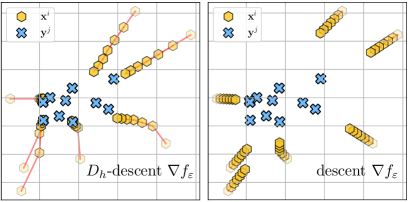
Figure 4: Difference between $W_{c}$ gradient descents, minimizing loss directly in direction $-\lambda\nabla f_{\varepsilon}$, or Bregman descent as described in Equation 17 when $h=\tfrac{1}{2}\ell_{2}^{2}+\ell_{1}$, see 4.1 for details on computing $\nabla h^{*}$. Six steps are plotted with stepsize $\lambda=\tfrac{1}{4}$.

4 Structured Monge Displacements

We introduce in this section cost functions $h$ that we call of elastic-type, namely functions with a $\ell_{2}^{2}$ term in addition to another function $\tau$. When $\tau$ is sparsity-inducing (minimized on sparse vectors, with kinks) and has a proximal operator in closed form, we show that the displacements induced by this function $h$ are feature-sparse.

4.1 Elastic-type Costs

By reference to (Zou and Hastie, 2005), we call $h$ of elastic-type if it is strongly convex and can be written as

$$h(\mathbf{z}):=\tfrac{1}{2}\|\mathbf{z}\|^{2}+\tau(\mathbf{z})\,.$$ (18)

where $\tau:\mathbb{R}^{d}\rightarrow\mathbb{R}$ is a function whose proximal operator is well-defined. Since OT algorithms are invariant to a positive rescaling of the cost $c$, our elastic-type costs subsume, without loss of generality, all strongly-convex translation invariant costs with convex $\tau$. They do also include useful cases arising when $\tau$ is not (e.g., $\tau_{\mathrm{stvs}}$).

Proposition 4.1.

For $h$ as in (18) and $\mathbf{x}\in\Omega_{\hat{\nu}_{m}}(\tau)$ one has:

$$T_{h,\varepsilon}(x):=\mathbf{x}-\operatorname{prox}_{\tau}\!\!\left(\!\mathbf{x}-\sum_{j=1}^{m}p^{\,j}(\mathbf{x})\left(\mathbf{y}^{j}+\nabla\tau(\mathbf{x}-\mathbf{y}^{j})\right)\!\!\right)$$ (19)

Proof.

The result follows from $\nabla h^{*}=\operatorname{prox}_{\tau}.$ Indeed:

$$h^{*}(\mathbf{w}) =\sup_{\mathbf{z}}\mathbf{w}^{T}\mathbf{z}-\tfrac{1}{2}\|\mathbf{z}\|^{2}-\tau(\mathbf{z})$$

$$=-\inf_{\mathbf{z}}-\mathbf{w}^{T}\mathbf{z}+\tfrac{1}{2}\|\mathbf{z}\|^{2}+\tau(\mathbf{z})$$

$$=\tfrac{1}{2}\|\mathbf{w}\|^{2}-\inf_{\mathbf{z}}\tfrac{1}{2}\|\mathbf{z}-\mathbf{w}\|^{2}+\tau(\mathbf{z}).$$

Differentiating on both sides and using Danskin’s lemma, we get the desired result by developing $\nabla h$ and taking advantage of the fact that the weights $p^{\,j}(\mathbf{x})$ sum to 1. ∎

4.2 Sparsity-Inducing Functions $\tau$

We discuss in this section the three choices we introduced in §2 for proximal operators and their practical implications in the context of our generalized entropic maps.

1-Norm $\ell_{1}$.

As a first example, we consider $\tau(\mathbf{z})=\gamma\|\mathbf{z}\|_{1}$ in Equation 18. The associated proximal operator is the soft-thresholding operator $\mathrm{prox}_{\tau}(\cdot)=\operatorname{ST}(\cdot,\gamma)$ mentioned in the introduction. We also have $\nabla h(\mathbf{z})=\mathbf{z}+\gamma\,\operatorname{sign}(\mathbf{z})$ for $\mathbf{z}$ with no $0$ coordinate. Plugging this in Equation 5, we find that the Monge map $T_{\gamma\ell_{1},\varepsilon}(\mathbf{x})$ is equal to

$$\mathbf{x}-\mathrm{ST}_{\gamma}\left(\mathbf{x}-\sum_{j=1}^{m}p^{\,j}(\mathbf{x})\left(\mathbf{y}^{j}+\gamma\operatorname{sign}(\mathbf{x}-\mathbf{y}^{j})\right)\right)\,,$$

where the $p^{\,j}(\mathbf{x})$ are evaluated at $\mathbf{x}$ using Equation 14. Applying the transport consists in an element-wise operation on $\mathbf{x}$: for each of its features $t\leq d$, one substracts $\mathrm{ST}_{\gamma}\left(\sum_{j=1}^{m}p^{\,j}(\mathbf{x})\nabla h(\mathbf{x}_{t}-\mathbf{y}^{j}_{t})\right)$. The only interaction between coordinates comes from the weights $p^{\,j}(\mathbf{x})$.

The soft-thresholding operator sparsifies the displacement. Indeed, when for a given $\mathbf{x}$ and a feature $t\leq d$ one has

$$|\mathbf{x}_{t}-\sum_{j=1}^{m}p^{\,j}(\mathbf{x})\mathbf{y}^{j}_{t}+\gamma\operatorname{sign}(\mathbf{x}_{t}-\mathbf{y}^{j}_{t})|\leq\gamma,$$

then there is no change on that feature : $[T_{\gamma\ell_{1},\varepsilon}(\mathbf{x})]_{t}=\mathbf{x}_{t}$. That mechanism works to produce, locally, sparse displacements on certain coordinates. Another interesting phenomenon happens when $\mathbf{x}$ is too far from the $\mathbf{y}_{j}$’s on some coordinates, in which case the transport defaults back to a $\ell_{2}^{2}$ average of the target points $\mathbf{y}^{j}$ (with weights that are, however, influenced by the $\gamma\ell_{1}$ regularization):

Proposition 4.2.

If $\mathbf{x}$ is such that $\mathbf{x}_{t}\geq\max_{j}\mathbf{y}^{j}_{t}$ or $\mathbf{x}_{t}\leq\min_{j}\mathbf{y}^{j}_{t}$ then $T_{\gamma\ell_{1},\varepsilon}(\mathbf{x})_{t}=\sum_{j}p^{\,j}(\mathbf{x})\mathbf{y}^{j}_{t}$.

Proof.

For instance, assume $\mathbf{x}_{t}\geq\max_{j}\mathbf{y}^{j}_{t}$. Then, for all $j$, we have $\mathrm{sign}(\mathbf{x}_{t}-\mathbf{y}^{j}_{t})=1$, and as a consequence $\sum_{j=1}^{m}p^{\,j}(\mathbf{x})\nabla h(\mathbf{x}-\mathbf{y}^{j})_{t}=\mathbf{x}_{t}-\sum_{j}p^{\,j}(\mathbf{x})\mathbf{y}^{j}_{t}+\gamma$. This quantity is greater than $\gamma$, so applying the soft-thresholding gives $\mathrm{ST}_{\gamma}(\sum_{j=1}^{m}p^{\,j}(\mathbf{x})\nabla h(\mathbf{x}-\mathbf{y}^{j})_{t})=\mathbf{x}_{t}-\sum_{j}p^{\,j}(\mathbf{x})\mathbf{y}^{j}_{t}$, which gives the advertised result. Similar reasoning gives the same result when $\mathbf{x}_{t}\leq\min_{j}\mathbf{y}^{j}_{t}$. ∎

Interestingly, this property depends on $\gamma$ only through the $p^{\,j}(\mathbf{x})$’s, and the condition that $\mathbf{x}_{t}\geq\max_{j}\mathbf{y}^{j}_{t}$ or $\mathbf{x}_{t}\leq\min_{j}\mathbf{y}^{j}_{t}$ does not depend on $\gamma$ at all.

Vanishing Shrinkage STVS:

The $\ell_{1}$ term added to form the elastic net has a well-documented drawback, notably for regression: on top of having a sparsifying effect on the displacement, it also shrinks values. This is clear from the soft-thresholding formula, where a coordinate greater than $\gamma$ is reduced by $\gamma$. This effect can lead to some “shortening” of displacement lengths in the entropic maps. We use the Soft-Thresholding with Vanishing Shrinkage (STVS) proposed by Schreck et al. (2015) to overcome this problem. The cost function is given by Equation 7, and its prox in Equation 8. When $|\mathbf{z}|$ is large, we have $\mathrm{prox}_{\tau_{\mathrm{stvs}}}(\mathbf{z})=\mathbf{z}+o(1)$, which means that the shrinkage indeed vanishes. Interestingly, even though the cost $\tau_{\mathrm{stvs}}$ is non-convex, it still has a proximal operator, and $\frac{1}{2}\|\cdot\|^{2}+\tau_{\mathrm{stvs}}$ is $\tfrac{1}{2}$-strongly convex.

$k$-Overlap: $\tau=\|\cdot\|_{\mathrm{ov}k}$.

The $k$-overlap norm offers the distinctive feature that its proximal operator selects anywhere between $d$ (small $\gamma$) and $k$ (large $\gamma$) non-zero variables, see Figure 1. Applying this proximal operator is, however, significantly more complex, because it is not separable across coordinates and requires $d(k+\log d)$ operations, instantiating a $k\times d-k$ matrix to select two integers $r,l$ ($r\leq k\leq l$) at each evaluation. We were able to use it for moderate problem sizes but these costs became prohibitive on larger scale datasets, where $d$ is a few tens of thousands.

5 Experiments

We start this experimental study with two synthetic tasks. For classic costs such as $\ell_{2}^{2}$, several examples of ground-truth optimal maps are known. Unfortunately, we do not know yet how to propose ground-truth $h$-optimal maps, nor dual potentials, when $h$ has the general structure considered in this work. As a result, we study two synthetic problems, where the sparsity pattern of a ground truth transport is either constant across $\mathbf{x}$ or split across two areas. We follow with an application to single-cell genomics, where the modeling assumption that a treatment has a sparse effect on gene activation (across $34k$ genes) is plausible. In terms of implementaiton, the entire pipeline described in § 3 and 4 rests on running the Sinkhorn algorithm first, with an appropriate cost, and than differentiating the resulting potentials. This can be carried out in a few lines of code using a parameterized TICost, fed into the Sinkhorn solver, to output a DualPotentials object in OTT-JAX(Cuturi et al., 2022). We a class of regularized translation invariant cost functions, specifying both regularizers $\tau$ and their proximal operators. We call such costs RegTICost.

5.1 Synthetic experiments.

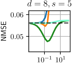
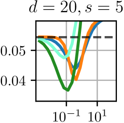
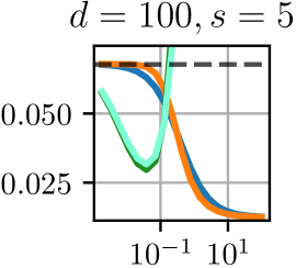
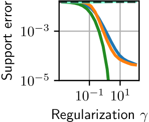
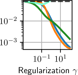
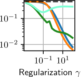
Figure 5: Synthetic experiment: ability of the estimated $T_{h,\varepsilon}$ to recover a ground-truth transport which displaces $s$ coordinates in dimension $d$, with $n=1000$ samples. We compare the different costs $h$ proposed in the paper with the classical $\ell_{2}^{2}$ cost. We identify $3$ regimes. Left: when $s\simeq d$, the $\ell_{2}^{2}$ cost is already good, and the proposed costs barely improve over it in terms of MSE. Middle: when $d$ is moderately larger than $s$, all the proposed costs improve over the $\ell_{2}^{2}$ cost, and the optimal regularization for $\ell_{1}$ and $\tau_{\mathrm{stvs}}$ are finite. Right: When $d\gg s$, the proposed methods vastly improve over the $\ell_{2}^{2}$ cost. The optimal regularization for $\ell_{1}$ and $\tau_{\mathrm{stvs}}$ is infinite even for the MSE. In terms of support error, larger regularization always leads to better results.

Constant sparsity-pattern. We measure the ability of our method to recover a sparse transport map using a setting inspired by (Pooladian and Niles-Weed, 2021). Here $\mu=\mathcal{U}_{[0,1]^{d}}$. For an integer $s<d$, we set $\nu=T^{\star}_{s}\sharp\mu$, where the map $T^{\star}_{s}$ acts on coordinates independently with the formula $T^{\star}_{s}(\mathbf{x})=[\exp(\mathbf{x}_{1}),\dots,\exp(\mathbf{x}_{s}),\mathbf{x}_{s+1},\dots,\mathbf{x}_{d}]$: it only changes the first $s$ coordinates of the vector, and corresponds to a sparse displacement when $s\ll d$. Note that this sparse transport plan is much simpler than the maps our model can handle since, for this synthetic example, the sparsity pattern is fixed across samples. Note also that while it might be possible to detect that only the first $s$ components have high variability using a 2-step pre-processing approach, or an adaptive, robust transport approach (Paty and Cuturi, 2019), our goal is to detect that support in a one-shot, thanks to our choice of $h$. We generate $n=1,000$ i.i.d. samples $\mathbf{x}^{i}$ from $\mu$, and $\mathbf{y}^{j}$ from $\nu$ independently; the samples $\mathbf{y}^{j}$ are obtained by first generating fresh i.i.d. samples $\tilde{\mathbf{x}}^{j}$ from $\mu$ and then pushing them : $\mathbf{y}^{j}:=T^{\star}_{s}(\tilde{\mathbf{x}}^{j})$. We use our three costs to compute $T_{h,\varepsilon}$ from these samples, and measure our ability to recover $T^{\star}_{s}$ from $T_{h,\varepsilon}$ using a normalized MSE defined as $\frac{1}{nd}\sum_{i=1}^{n}\|T^{\star}_{s}(\mathbf{x}^{i})-T_{h,\varepsilon}(\mathbf{x}^{i})\|^{2}$. We also measure how well our method identifies the correct support: for each sample, we compute the support error as $\sum_{i=s+1}^{d}\mathbf{\Delta}_{i}^{2}/\sum_{i=1}^{d}\mathbf{\Delta}_{i}^{2}$ with $\mathbf{\Delta}$ the displacement $T_{h,\varepsilon}(\mathbf{x})-\mathbf{x}$. This quantity is between $0$ and $1$ and cancels if and only if the displacement happens only on the correct coordinates. We then average this quantity overall the $\mathbf{x}^{i}$. Figure 5 displays the results as $d$ varies and $s$ is fixed. Here, $\tau_{\mathrm{stvs}}$ performs better than $\ell_{1}$.

$\mathbf{x}$-dependent sparsity-pattern. To illustrate the ability of our method to recover transport maps whose sparsity pattern is adaptive, depending depending on the input $\mathbf{x}$, we extend the previous setting as follows. To compute $F_{s}(\mathbf{x})$, we compute first the norms of two coordinate groups of $\mathbf{x}$: $n_{1}=\sum_{i=1}^{s}\mathbf{x}_{i}^{2}$ and $n_{2}=\sum_{i=s+1}^{2s}\mathbf{x}_{i}^{2}$. Second, we displace the coordinate group with the largest norm: if $n_{1}>n_{2}$, $F_{s}(\mathbf{x})=[\exp(\mathbf{x}_{1}),\dots,\exp(\mathbf{x}_{s}),\mathbf{x}_{s+1},\dots,\mathbf{x}_{d}]$, otherwise $F_{s}(\mathbf{x})=[\mathbf{x}_{1},\dots,\mathbf{x}_{s},\exp(\mathbf{x}_{s+1}),\dots,\exp(\mathbf{x}_{2s}),\mathbf{x}_{2s+1},\dots,\mathbf{x}_{d}]$. Obviously, the displacement pattern depends on $\mathbf{x}$. Figure 6 shows the NMSE with different costs when the dimension $d$ increases while $s$ and $n$ are fixed. As expected, we observe a much better scaling for our costs than for the standard $\ell^{2}_{2}$ cost, indicating that sparsity-inducing costs mitigate the curse of dimensionality.

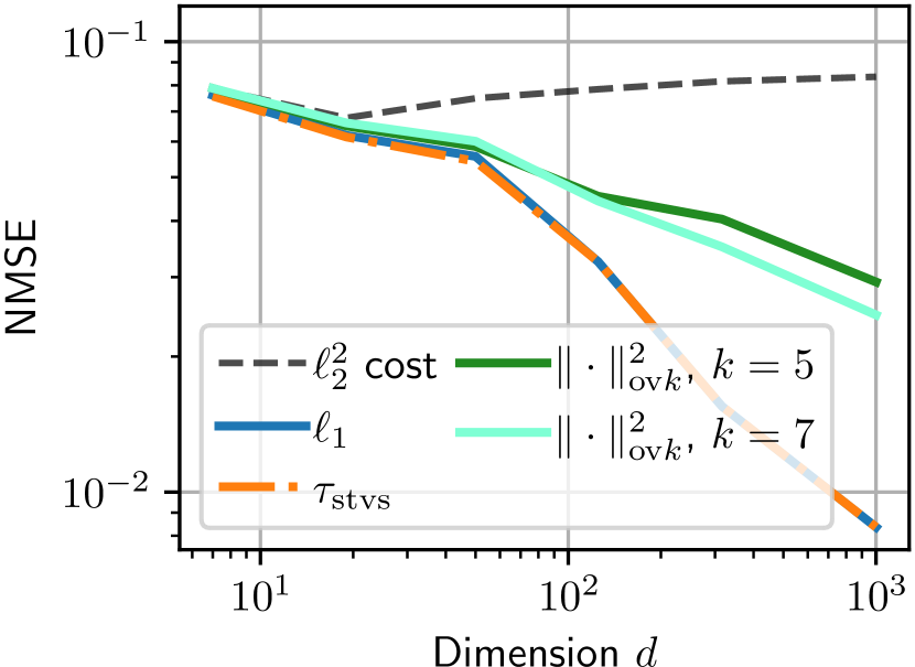
Figure 6: Scaling with dimension: The number of samples is fixed to $n=100$, and the sparsity to $s=2$. For each dimension, we do a grid search over $\gamma$ and retain the one with the lowest MSE.

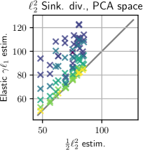
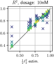
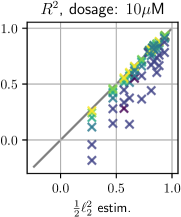
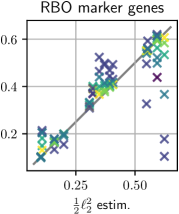
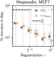
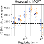
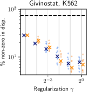
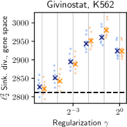
Figure 7: Top row: performance, for all 15 experiments, of the elastic-$\gamma\ell_{1}$ estimator vs. the $\tfrac{1}{2}\ell_{2}^{2}$ entropic map. We consider 6 values for $\gamma$. Each of the $15\times 6$ crosses denotes the mean, over 10 random 80%,/20% splits of that cell line/drug experiment, of a quantity of interest. To facilitate reading, rather than reporting the $\gamma$ value, we report the average percentage of non-zero displacements (using np.isclose(.,0), equivalently thresholding values below $10^{-8}$) across all displaced points in that fold (yellow means $40\%$ dense displacements, dark-blue displacements only happen on $\approx 5\%$ of genes). While all these maps are estimated in full genes space ($\approx 34k$), we provide a simplified measure of their ability to reconstruct the measures by computing a $\tfrac{1}{2}\ell_{2}^{2}$-Sinkhorn divergence in PCA space. This picture shows that one can sparsify significantly $\tfrac{1}{2}\ell_{2}^{2}$ maps and still get a similar reconstruction error. Next, we picture separately the $R^{2}$ (see text body for details) computed on marker genes on low ($10nM$) and high ($10\mu M$) dosages of the drug. For low dosages, inducing sparsity in displacements seems to help, whereas this may no longer be the case when the effect of perturbations becomes large. Finally, the RBO metric shows that sparsity does help to select marker genes based only on map estimation. Bottom row: Close up on Hesperadin/MCF7 and Givinostat/K562 experiments. For each, we quantify the sparsifying effect w.r.t $\gamma$, as well as $\tfrac{1}{2}\ell_{2}^{2}$-Sinkhorn divergence in full gene space.

5.2 Single-Cell RNA-seq data.

We validate our approach on the single-cell RNA sequencing perturbation data from (Srivatsan et al., 2020). After removing cells with less than $200$ expressed genes and genes expressed in less than $20$ cells, the data consists of $579,483$ cells and $34,636$ genes. In addition, the raw counts have been normalized and $\log(x+1)$ scaled. We select the $5$ drugs (Belinostat, Dacinostat, Givinostat, Hesperadin, and Quisinostat) out of $188$ drug perturbations that are highlighted in the original data (Srivatsan et al., 2020) as showing a strong effect. We consider $3$ human cancer cell lines (A549, K562, MCF7) to each of which is applied each of the $5$ drugs. We use our four methods to learn an OT map from control to perturbed cells in each of these $3\times 5$ scenarios. For each cell line/drug pair, we split the data into $10$ non-overlapping 80%/20% train/test splits, keeping the test fold to produce our metrics.

Table 1: Per cell line, sample sizes of control + drug perturbation.

	Cont.	Dac.	Giv.	Bel.	Hes.	Quis.
A549	3274	558	703	669	436	475
K562	3346	388	589	656	624	339
MCF7	6346	1562	1805	1684	882	1520

Methods. We ran experiments in two settings, using the whole $34,000$-$d$ gene space and subsetting to the top $5k$ highly variable genes using ScanPy (Wolf et al., 2018). We consider entropic map estimators with the following cost functions and pre-processing approaches: $\tfrac{1}{2}\ell_{2}^{2}$ cost; the $\tfrac{1}{2}\ell_{2}^{2}$ cost on $50$-$d$ PCA space (PCA directions are recomputed on each train fold); Elastic with $\gamma\ell_{1}$; Elastic with $\gamma$-$\tau_{\mathrm{svts}}$ cost. We vary $\gamma$ for these two methods. We did not use the $\|\cdot\|_{\mathrm{ov}k}$ norm because of memory challenges when handling such a high-dimensional dataset. For the non-PCA-based approaches, we can also measure their performance in PCA space by projecting their high-dimensional predictions onto the 50-$d$ space. The $\varepsilon$ regularization parameter for all these approaches is set for each cost and experiment to $10\%$ of the mean value of the cost matrix between the train folds of control and treated cells, respectively.

Evaluation. We evaluate methods using these metrics:

• the $\ell_{2}^{2}$-Sinkhorn divergence (using $\varepsilon$ to be 10% of the mean of pairwise $\ell_{2}^{2}$ cost matrix of treated cells) between transferred points (from test fold of control) and test points (from perturbed state); lower is better.

• Ranked biased overlap (Webber et al., 2010) with $p=0.9$, between the $50$ perturbation marker genes as computed on all data with ScanPy, and the following per-gene statistic, computed using a map as follows: average (on fold) expression of (predicted) perturbed cells from original control cells (this tracks changes in log-expression before/after predicted treatment); higher is better.

• Coefficient of determination ($R^{2}$) between the average ground-truth / predicted gene expression on the $50$ perturbation markers (Lotfollahi et al., 2019); higher is better.

These results are summarized in Figure 7, across various costs, perturbations and hyperparameter choices.

Conclusion. We consider structured translation-invariant ground costs $h$ for transport problems. After forming an entropic potential with such costs, we plugged it in Brenier’s approach to construct a generalized entropic map. We highlighted a surprising connection between that map and the Bregman centroids associated with the divergence generated by $h$, resulting in a more natural approach to gradient flows defined by $W_{c}$, illustrated in a simple example. By selecting costs $h$ of elastic type (a sum of $\ell_{2}^{2}$ and a sparsifying term), we show that our maps mechanically exhibit sparsity, in the sense that they have the ability to only impact adaptively $\mathbf{x}$ on a subset of coordinates. We have proposed two simple generative models where this property helps estimation and applied this approach to high-dimensional single-cell datasets where we show, at a purely mechanical level, that we can recover meaningful maps. Many natural extensions of our work arise, starting with more informative sparsity-inducing norms (e.g., group lasso), and a more general approach leveraging the Bregman geometry for more ambitious $W_{c}$ problems, such as barycenters.

References

- Ambrosio and Pratelli (2003) Luigi Ambrosio and Aldo Pratelli. Existence and stability results in the l1 theory of optimal transportation. Optimal Transportation and Applications: Lectures given at the CIME Summer School, held in Martina Franca, Italy, September 2-8, 2001, pages 123–160, 2003.
- Ambrosio et al. (2004) Luigi Ambrosio, Bernd Kirchheim, and Aldo Pratelli. Existence of optimal transport maps for crystalline norms. Duke Mathematical Journal, 125(2):207–241, 2004.
- Argyriou et al. (2012) Andreas Argyriou, Rina Foygel, and Nathan Srebro. Sparse prediction with the k-support norm. In F. Pereira, C.J. Burges, L. Bottou, and K.Q. Weinberger, editors, Advances in Neural Information Processing Systems, volume 25. Curran Associates, Inc., 2012.
- Arjovsky et al. (2017) Martin Arjovsky, Soumith Chintala, and Léon Bottou. Wasserstein gan. arXiv preprint arXiv:1701.07875, 2017.
- Bach et al. (2012) Francis Bach, Rodolphe Jenatton, Julien Mairal, Guillaume Obozinski, et al. Optimization with sparsity-inducing penalties. Foundations and Trends® in Machine Learning, 4(1):1–106, 2012.
- Bianchini and Bardelloni (2014) Stefano Bianchini and Mauro Bardelloni. The decomposition of optimal transportation problems with convex cost. arXiv preprint arXiv:1409.0515, 2014.
- Blondel et al. (2018) Mathieu Blondel, Vivien Seguy, and Antoine Rolet. Smooth and sparse optimal transport. In International conference on artificial intelligence and statistics, pages 880–889. PMLR, 2018.
- Bonneel et al. (2015) Nicolas Bonneel, Julien Rabin, Gabriel Peyré, and Hanspeter Pfister. Sliced and radon wasserstein barycenters of measures. Journal of Mathematical Imaging and Vision, 51:22–45, 2015.
- Brenier (1991) Yann Brenier. Polar factorization and monotone rearrangement of vector-valued functions. Comm. Pure Appl. Math., 44(4):375–417, 1991. ISSN 0010-3640. doi: 10.1002/cpa.3160440402. URL https://doi.org/10.1002/cpa.3160440402.
- Carlier et al. (2010) Guillaume Carlier, Luigi De Pascale, and Filippo Santambrogio. A strategy for non-strictly convex transport costs and the example of in . Communications in Mathematical Sciences, 8(4):931–941, 2010.
- Courty et al. (2016) Nicolas Courty, Rémi Flamary, Devis Tuia, and Alain Rakotomamonjy. Optimal transport for domain adaptation. IEEE transactions on pattern analysis and machine intelligence, 39(9):1853–1865, 2016.
- Courty et al. (2017) Nicolas Courty, Rémi Flamary, Amaury Habrard, and Alain Rakotomamonjy. Joint distribution optimal transportation for domain adaptation. Advances in Neural Information Processing Systems, 30, 2017.
- Cuturi (2013) Marco Cuturi. Sinkhorn distances: Lightspeed computation of optimal transport. In Advances in neural information processing systems, pages 2292–2300, 2013.
- Cuturi and Doucet (2014) Marco Cuturi and Arnaud Doucet. Fast computation of wasserstein barycenters. In Eric P. Xing and Tony Jebara, editors, Proceedings of the 31st International Conference on Machine Learning, volume 32 of Proceedings of Machine Learning Research, pages 685–693, Bejing, China, 22–24 Jun 2014. PMLR. URL https://proceedings.mlr.press/v32/cuturi14.html.
- Cuturi et al. (2022) Marco Cuturi, Laetitia Meng-Papaxanthos, Yingtao Tian, Charlotte Bunne, Geoff Davis, and Olivier Teboul. Optimal transport tools (ott): A jax toolbox for all things wasserstein. arXiv preprint arXiv:2201.12324, 2022.
- Deshpande et al. (2019) Ishan Deshpande, Yuan-Ting Hu, Ruoyu Sun, Ayis Pyrros, Nasir Siddiqui, Sanmi Koyejo, Zhizhen Zhao, David Forsyth, and Alexander G Schwing. Max-sliced wasserstein distance and its use for gans. In Proceedings of the IEEE/CVF Conference on Computer Vision and Pattern Recognition, pages 10648–10656, 2019.
- Dessein et al. (2018) Arnaud Dessein, Nicolas Papadakis, and Jean-Luc Rouas. Regularized optimal transport and the rot mover’s distance. The Journal of Machine Learning Research, 19(1):590–642, 2018.
- Dudley et al. (1966) Richard Mansfield Dudley et al. Weak convergence of probabilities on nonseparable metric spaces and empirical measures on euclidean spaces. Illinois Journal of Mathematics, 10(1):109–126, 1966.
- Evans and Gangbo (1999) Lawrence C Evans and Wilfrid Gangbo. Differential equations methods for the Monge-Kantorovich mass transfer problem. American Mathematical Soc., 1999.
- Feydy et al. (2019) Jean Feydy, Thibault Séjourné, François-Xavier Vialard, Shun-ichi Amari, Alain Trouvé, and Gabriel Peyré. Interpolating between optimal transport and mmd using sinkhorn divergences. In The 22nd International Conference on Artificial Intelligence and Statistics, pages 2681–2690. PMLR, 2019.
- Genevay et al. (2018) Aude Genevay, Gabriel Peyré, and Marco Cuturi. Learning generative models with Sinkhorn divergences. In Proceedings of the 21st International Conference on Artificial Intelligence and Statistics, pages 1608–1617, 2018.
- Hastie et al. (2015) Trevor Hastie, Robert Tibshirani, and Martin Wainwright. Statistical learning with sparsity. Monographs on statistics and applied probability, 143:143, 2015.
- Huang et al. (2021) Minhui Huang, Shiqian Ma, and Lifeng Lai. A riemannian block coordinate descent method for computing the projection robust wasserstein distance. In Marina Meila and Tong Zhang, editors, Proceedings of the 38th International Conference on Machine Learning, volume 139 of Proceedings of Machine Learning Research, pages 4446–4455. PMLR, 18–24 Jul 2021.
- Janati et al. (2019) Hicham Janati, Marco Cuturi, and Alexandre Gramfort. Wasserstein regularization for sparse multi-task regression. In The 22nd International Conference on Artificial Intelligence and Statistics, pages 1407–1416. PMLR, 2019.
- Kiwiel (1997) Krzysztof C Kiwiel. Proximal minimization methods with generalized bregman functions. SIAM journal on control and optimization, 35(4):1142–1168, 1997.
- Kolouri et al. (2019) Soheil Kolouri, Kimia Nadjahi, Umut Simsekli, Roland Badeau, and Gustavo Rohde. Generalized sliced wasserstein distances. Advances in neural information processing systems, 32, 2019.
- Korotin et al. (2020) Alexander Korotin, Vage Egiazarian, Arip Asadulaev, Alexander Safin, and Evgeny Burnaev. Wasserstein-2 generative networks. In International Conference on Learning Representations, 2020.
- Le et al. (2019) Tam Le, Makoto Yamada, Kenji Fukumizu, and Marco Cuturi. Tree-sliced variants of wasserstein distances. Advances in neural information processing systems, 32, 2019.
- Lin et al. (2020) Tianyi Lin, Chenyou Fan, Nhat Ho, Marco Cuturi, and Michael Jordan. Projection robust wasserstein distance and riemannian optimization. Advances in neural information processing systems, 33:9383–9397, 2020.
- Lin et al. (2021) Tianyi Lin, Zeyu Zheng, Elynn Chen, Marco Cuturi, and Michael I Jordan. On projection robust optimal transport: Sample complexity and model misspecification. In International Conference on Artificial Intelligence and Statistics, pages 262–270. PMLR, 2021.
- Liu et al. (2022) Tianlin Liu, Joan Puigcerver, and Mathieu Blondel. Sparsity-constrained optimal transport. arXiv preprint arXiv:2209.15466, 2022.
- Lotfollahi et al. (2019) Mohammad Lotfollahi, F. Alexander Wolf, and Fabian J. Theis. scgen predicts single-cell perturbation responses. Nature Methods, 16(8):715–721, Aug 2019. ISSN 1548-7105. doi: 10.1038/s41592-019-0494-8. URL https://doi.org/10.1038/s41592-019-0494-8.
- Makkuva et al. (2020) Ashok Makkuva, Amirhossein Taghvaei, Sewoong Oh, and Jason Lee. Optimal transport mapping via input convex neural networks. In International Conference on Machine Learning, pages 6672–6681. PMLR, 2020.
- Monge (1781) Gaspard Monge. Mémoire sur la théorie des déblais et des remblais. Histoire de l’Académie Royale des Sciences, pages 666–704, 1781.
- Montavon et al. (2016) Grégoire Montavon, Klaus-Robert Müller, and Marco Cuturi. Wasserstein training of restricted boltzmann machines. In D. Lee, M. Sugiyama, U. Luxburg, I. Guyon, and R. Garnett, editors, Advances in Neural Information Processing Systems, volume 29. Curran Associates, Inc., 2016.
- Muzellec and Cuturi (2019) Boris Muzellec and Marco Cuturi. Subspace detours: Building transport plans that are optimal on subspace projections. In H. Wallach, H. Larochelle, A. Beygelzimer, F. d'Alché-Buc, E. Fox, and R. Garnett, editors, Advances in Neural Information Processing Systems, volume 32. Curran Associates, Inc., 2019.
- Nielsen and Nock (2009) Frank Nielsen and Richard Nock. Sided and symmetrized bregman centroids. IEEE Transactions on Information Theory, 55(6):2882–2904, 2009. doi: 10.1109/TIT.2009.2018176.
- Niles-Weed and Rigollet (2022) Jonathan Niles-Weed and Philippe Rigollet. Estimation of wasserstein distances in the spiked transport model. Bernoulli, 28(4):2663–2688, 2022.
- Paty and Cuturi (2019) François-Pierre Paty and Marco Cuturi. Subspace robust wasserstein distances. arXiv preprint arXiv:1901.08949, 2019.
- Peyré and Cuturi (2019) Gabriel Peyré and Marco Cuturi. Computational optimal transport. Foundations and Trends® in Machine Learning, 11(5-6):355–607, 2019.
- Peyré and Cuturi (2019) Gabriel Peyré and Marco Cuturi. Computational optimal transport. Foundations and Trends in Machine Learning, 11(5-6), 2019. ISSN 1935-8245.
- Pooladian and Niles-Weed (2021) Aram-Alexandre Pooladian and Jonathan Niles-Weed. Entropic estimation of optimal transport maps. arXiv preprint arXiv:2109.12004, 2021.
- Rabin et al. (2012) Julien Rabin, Gabriel Peyré, Julie Delon, and Marc Bernot. Wasserstein barycenter and its application to texture mixing. In Scale Space and Variational Methods in Computer Vision: Third International Conference, SSVM 2011, Ein-Gedi, Israel, May 29–June 2, 2011, Revised Selected Papers 3, pages 435–446. Springer, 2012.
- Rigollet and Stromme (2022) Philippe Rigollet and Austin J Stromme. On the sample complexity of entropic optimal transport. arXiv preprint arXiv:2206.13472, 2022.
- Salimans et al. (2018) Tim Salimans, Han Zhang, Alec Radford, and Dimitris Metaxas. Improving GANs using optimal transport. In International Conference on Learning Representations, 2018.
- Santambrogio (2015) Filippo Santambrogio. Optimal transport for applied mathematicians. Springer, 2015.
- Schiebinger et al. (2019) Geoffrey Schiebinger, Jian Shu, Marcin Tabaka, Brian Cleary, Vidya Subramanian, Aryeh Solomon, Joshua Gould, Siyan Liu, Stacie Lin, Peter Berube, et al. Optimal-transport analysis of single-cell gene expression identifies developmental trajectories in reprogramming. Cell, 176(4):928–943, 2019.
- Schreck et al. (2015) Amandine Schreck, Gersende Fort, Sylvain Le Corff, and Eric Moulines. A shrinkage-thresholding metropolis adjusted langevin algorithm for bayesian variable selection. IEEE Journal of Selected Topics in Signal Processing, 10(2):366–375, 2015.
- Sinkhorn (1964) Richard Sinkhorn. A relationship between arbitrary positive matrices and doubly stochastic matrices. Ann. Math. Statist., 35:876–879, 1964.
- Srivatsan et al. (2020) Sanjay R. Srivatsan, José L. McFaline-Figueroa, Vijay Ramani, Lauren Saunders, Junyue Cao, Jonathan Packer, Hannah A. Pliner, Dana L. Jackson, Riza M. Daza, Lena Christiansen, Fan Zhang, Frank Steemers, Jay Shendure, and Cole Trapnell. Massively multiplex chemical transcriptomics at single-cell resolution. Science, 367(6473):45–51, 2020. doi: 10.1126/science.aax6234. URL https://www.science.org/doi/abs/10.1126/science.aax6234.
- Sudakov (1979) Vladimir N Sudakov. Geometric problems in the theory of infinite-dimensional probability distributions. Number 141. American Mathematical Soc., 1979.
- Telgarsky and Dasgupta (2012) Matus Telgarsky and Sanjoy Dasgupta. Agglomerative bregman clustering. In Proceedings of the 29th International Conference on Machine Learning, ICML 2012, Edinburgh, Scotland, UK, June 26 - July 1, 2012. icml.cc / Omnipress, 2012.
- Trudinger and Wang (2001) Neil S Trudinger and Xu-Jia Wang. On the monge mass transfer problem. Calculus of Variations and Partial Differential Equations, 13(1):19–31, 2001.
- Webber et al. (2010) William Webber, Alistair Moffat, and Justin Zobel. A similarity measure for indefinite rankings. ACM Transactions on Information Systems (TOIS), 28(4):1–38, 2010.
- Weed and Bach (2019) Jonathan Weed and Francis Bach. Sharp asymptotic and finite-sample rates of convergence of empirical measures in wasserstein distance. Bernoulli, 25(4A):2620–2648, 2019.
- Wolf et al. (2018) F Alexander Wolf, Philipp Angerer, and Fabian J Theis. Scanpy: large-scale single-cell gene expression data analysis. Genome biology, 19(1):1–5, 2018.
- Zou and Hastie (2005) Hui Zou and Trevor Hastie. Regularization and variable selection via the elastic net. Journal of the royal statistical society: series B (statistical methodology), 67(2):301–320, 2005.