Weakly-supervised Representation Learning for Video Alignment and Analysis

Abstract

Many tasks in video analysis and understanding boil down to the need for frame-based feature learning, aiming to encapsulate the relevant visual content so as to enable simpler and easier subsequent processing. While supervised strategies for this learning task can be envisioned, self and weakly-supervised alternatives are preferred due to the difficulties in getting labeled data. This paper introduces LRProp – a novel weakly-supervised representation learning approach, with an emphasis on the application of temporal alignment between pairs of videos of the same action category. The proposed approach uses a transformer encoder for extracting frame-level features, and employs the DTW algorithm within the training iterations in order to identify the alignment path between video pairs. Through a process referred to as “pair-wise position propagation”, the probability distributions of these correspondences per location are matched with the similarity of the frame-level features via KL-divergence minimization. The proposed algorithm uses also a regularized SoftDTW loss for better tuning the learned features. Our novel representation learning paradigm consistently outperforms the state of the art on temporal alignment tasks, establishing a new performance bar over several downstream video analysis applications.

1 Introduction

As in many other domains, deep learning techniques have brought a revolution to the field of video analysis and understanding in the past several years [1, 2, 3]. Applications such as video classification [4, 5, 6], action detection [7, 8, 9], video captioning [10, 11], forecasting [12, 13], and many others, all have been getting new and highly effective AI-based solutions with unprecedented performance. Interestingly, within this impressive progress, the task of temporal alignment of video pairs has received relatively little attention. This paper offers a novel weakly-supervised approach towards representation learning for video, focusing on the temporal alignment application.

Many events occur in a specific temporal sequence, such as specific actions in sport activity (e.g., baseball swing), portions of a person’s daily routine, various repetitive medical procedures, sea tides, intervals within traffic control videos, or even simple actions such as pouring a glass of fluid. In all these and other cases, videos that capture such visual content contain not only information about the cause and effect of these events, but also the potential for temporal correspondences across multiple instances of the same process. For example, the key moment of reaching for a container and lifting it off the ground are common to all pouring sequences, despite differences in visual factors such as container style, illumination, surrounding items, and event speed. Broadly speaking, a reliable alignment of such videos can open the door to new abilities in video analysis, such as detecting anomaly behavior, enabling quick search of specific sub-events, identifying the phase within the whole event, measuring distances between videos for their clustering, and so much more.

So, how can videos be aligned? Earlier work [14, 15, 16] suggests to address this task by first learning spatio-temporal feature representations for each video frame. Given such representations, their sequential matching over time, which takes into account temporal correspondences, would result in the desired alignment [15, 17, 18]. This temporal matching could be achieved in a variety of ways, ranging from the simple nearest neighbor search, all the way to Dynamic Time Warping, DTW [19]. The sought representations should capture key visual information while discarding irrelevant details, and do this while also providing a dimensionality reduction for ease of later processing.

Representation learning could be achieved in a supervised fashion when frame-by-frame alignment is readily available. In this case, our task simply involves learning a common embedding space from pairs of aligned frames. A few approaches have been proposed for such supervised action recognition and segmentation [20, 21, 22]. However, in many real-world sequences, such frame-by-frame alignment does not exist naturally. Obtaining labels for every frame in a video might be time-consuming and ill-defined task, as it is unclear what set of labels would be necessary for a complete understanding of the fine-grained details of the video. A possible remedy to the above could be to artificially obtain aligned sequences by recording the same event from multiple cameras, but this method may not capture all the variations present in naturally occurring videos. All this brings us to self - or weak-supervision alternatives, as practiced in [16, 18]. These methods may rely on video augmentation or use a SoftDTW [23] loss for training the representations.

Inspired by the above described work, we present LRProp (Learning Representations by position PROPagation) – a novel weakly-supervised approach that does not require explicit frame correspondences between different video sequences. To accomplish our goal, we adopt the transformer encoder [24], which has demonstrated effectiveness in extracting meaningful frame-level features, as shown in [16, 25, 26]. Our experiments suggest that the transformer encoder is particularly beneficial for video alignment, and we believe that this is due to its positional encoding. In each step within the learning process, our method involves taking pairs of videos that depict the same action category, feeding them into the transformer encoder to generate frame-level features, and using the DTW algorithm [19] to produce a path aligning the two. We use this alignment path to define a pair-wise position propagation (definitions follow), which we utilize to establish a soft one-to-one linkage between pairs of frames. This pair-wise position propagation is used to define a prior distribution for the correspondence between two distinct frames from different videos, and we minimize the KL-divergence between this prior and a probability distribution over the similarity of the frame-level features (extracted by the transformer encoder) of the specified pair of frames. Our learning also employs the SoftDTW algorithm [23] with appropriate regularization to prevent trivial solutions, and to learn a more accurate alignment path for pairs of videos. Figure 1 demonstrates temporal alignment using the features extracted by the proposed method.

To summarize, our contributions include the following:

• We present a general weakly-supervised framework for learning frame-wise representations with a focus on video alignment.

• The proposed pair-wise position propagation is shown to result in features that offer better temporal awareness compared to prior work.

• Our approach achieves superior performance to the state-of-the-art on various temporal understanding tasks on the Pouring [27] and PennAction [28] datasets, setting a new performance benchmark for downstream tasks.

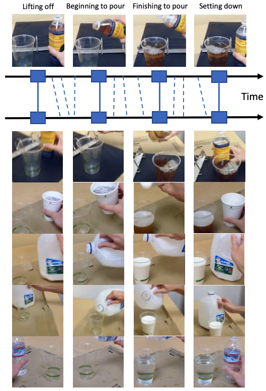
Figure 1: Video alignment (Pouring dataset) using LRProp features and the DTW algorithm. The first row shows a selected set of key events in a randomly selected video; the bottom shows the alignment results of these events with five other randomly chosen videos. As can be seen, LRProp leads to a successful capture of the key events in the query. Note that we show a single time-line for all the five selected videos for simplicity.

2 Related Work

Since labeled data can be expensive and time-consuming to collect and annotate, and may not always be available in sufficient quantities for certain tasks, self-supervised learning has become a widely studied area in the field of deep learning. As a result, numerous pretext tasks have been proposed for image-based methods to achieve self-supervision. These include relative patch prediction [29], jigsaw puzzle solving [30], colorization [31], rotation prediction [32], instance discrimination using strong data augmentation [33], knowledge distillation [34, 35], and more. These methods and many others have been shown to be highly effective in various downstream tasks. In this study, we investigate the use of self-supervised and weakly-supervised (definitions follow) learning techniques to create representations from videos, taking advantage of both the spatial and temporal information contained within the video data.

As we transition from images to video, various supporting tasks that produce supervision signals have been employed in representation learning for video frames. These include predicting the sequence of frames in a video [36, 37] or predicting audio from video [38]. Recently, the incorporation of temporal ordering has been demonstrated to be a strong pretext task to obtain meaningful video representations. Sermanet et al. [27] proposed Time-Contrastive Networks (TCN), which uses attraction and repulsion between temporally close and far frames, respectively, in order to learn useful features. Sal [14] proposed to learn features by sampling tuples of frames and predicting whether the tuple is in the correct temporal order (obtaining the labels using the frame indices). Another closely related work (TCC) was proposed by [15], which learns representations by finding frame correspondences across videos.

In this context, we should mention two recent works, SCL and VAVA [16, 39], which also achieved impressive results in self-supervised learning for videos. Chen et al. [16] proposed strongly augmenting the input both temporally and spatially, and using a transformer model [24] as an encoder, which has been used for videos in recent works [25, 26]. They also used a contrastive loss function to encourage the embedding of nearby frames to be more similar than those that are far apart. Liu et al. [39] attempted to learn video representations while considering the possibility of background frames, redundant frames, and non-monotonic frames when aligning two videos in time.

Whereas some work, as the above, assumes a self-supervised setting, in this paper we consider a weakly-supervised alternative, as described in [40]. More specifically, we refer to cases in which the videos of interest consist of the same action category sequence. In these cases, we are given an ordered list of actions during training, but the exact temporal boundaries or paste of each action are not provided. For example, in a video of pouring wine, the weak supervision might include the sequence “take the bottle, pour the wine, place the bottle back.” This leads us to a powerful pretext task known as temporal video alignment, in which multitude of such corresponding videos can be leveraged for supervised learning.

Though there is a significant amount of literature on time series alignment, only a few of these ideas have been applied to aligning videos. While traditional methods for time series alignment, such as DTW [19], are not differentiable and therefore cannot be used directly for training neural networks, a smooth approximation of DTW, called SoftDTW, was introduced in [23]. Several recent papers [41, 18] attempted to apply a soft DTW approximation in video representations learning. As an example, we mention Haresh et al. [18], which introduced a technique called LAV (Learning by Aligning Videos in Time) for learning representative frame embeddings by aligning videos in time using SoftDTW during training. However, their method, and other methods that use a soft DTW approximation during training, do not take advantage of the alignment path explicitly during optimization. In contrast, our approach, as unfolded in the next section, integrates both the SoftDTW cost function and the DTW alignment path into the optimization process.

3 Method

In this section we present Learning Representations by position PROPagation, LRProp, a framework for learning frame-wise video representations. We learn an embedding space where videos with similar content can be aligned in time; this setting is commonly referred to as weakly-supervised learning, as discussed in Section 2. More specifically, our method involves taking pairs of videos that depict the same action category, feeding them into the transformer encoder to generate frame-level features for each, and using the DTW algorithm [19] to produce a path aligning the two. We use this alignment to define a pair-wise position propagation, and establish a soft one-to-one linkage between pairs of frames. We minimize the KL-divergence between a reference distribution and the probability function over the similarity of the frame-level features of the specified pairs of frames. We also use the SoftDTW algorithm [23] with appropriate regularization to prevent trivial solutions as part of our training process. A visualization of our pair-wise position propagation method is depicted in Figure 2. In what follows, we detail each of the above-described ingredients.

3.1 Notations and Definitions

We begin by introducing the necessary notations and definitions for our discussion. Let $\mathcal{V}^{1}$ and $\mathcal{V}^{2}$ be a pair of videos, where each is represented as $\mathcal{V}^{i}\in\mathbf{R}^{F_{i}\times C\times W\times H}$. Here, $F_{i}$ represents the number of frames in the $i$th video and $C$, $W$, and $H$ are the number of channels, width, and height of each frame, respectively. To begin, we perform the same random sampling and data augmentation process described in [16]. This process takes a video $\mathcal{V}^{i}$ and uses temporal random cropping to generate two cropped videos of length $T$, $(V^{i}_{1},S_{1}^{i})$ and $(V^{i}_{2},S^{i}_{2})$, where $T$ is a hyper-parameter, and $S^{i}_{1/2}$ hold the frame indices. Next, several temporal-consistent spatial data augmentations are performed on each of the two sampled videos. After this step on $\mathcal{V}^{1}$ and $\mathcal{V}^{2}$, we are left with $(V^{1}_{1},S^{1}_{1}),(V^{1}_{2},S^{1}_{2})$, and $(V^{2}_{1},S^{2}_{1}),(V_{2}^{2},S_{2}^{2})$. We will use hereafter capital Latin letters to index the different videos, and greek letters to index the samplings.

We define a neural model, $f_{\theta}:\mathbf{R}^{T\times C\times W\times H}\rightarrow\mathcal{Z}$, which maps videos from an input space to an embedding space $\mathcal{Z}$. We adapt the transformer model [24] used by [16]. Assuming the existence of a prior distribution that represents the similarity between a frame, indexed $[S^{\mathrm{A}}_{\alpha}]_{i}$, and a given frame, indexed $[S^{\mathrm{B}}_{\beta}]_{j}$, which we define by $p_{\mathrm{A},\mathrm{B},\alpha,\beta}(i|j)$, our goal is to enforce the model’s embedding ($f_{\theta}(V)\triangleq Z$) similarity to follow this distribution. We propose to achieve this by minimizing the KL-divergence between $p$ and the following distribution:

$$q_{\theta,\mathrm{A},\mathrm{B},\alpha,\beta}(i|j)\equiv\mathcal{Q}_{\theta}(i|j)=\frac{\text{exp}(\text{sim}([Z^{\mathrm{B}}_{\beta}]_{j},[Z^{\mathrm{A}}_{\alpha}]_{i})/\tau)}{\sum_{i^{\prime}=1}^{T}\text{exp}(\text{sim}([Z^{\mathrm{B}}_{\beta}]_{j},[Z^{\mathrm{A}}_{\alpha}]_{i^{{}^{\prime}}})/\tau)},$$ (1)

where sim denotes the cosine similarity ($\text{sim}(\mathbf{u},\mathbf{v})=\mathbf{u}^{T}\mathbf{v}/\lVert\mathbf{u}\rVert\lVert\mathbf{v}\rVert$) and $\tau$ is a hyper-parameter controlling the smoothness of the distribution. The question remains, what would be a good prior for a given pair of videos?

3.2 Prior Distribution for Frames in the Same Video

Let $(Z^{\mathrm{A}}_{\alpha},S^{\mathrm{A}}_{\alpha}),(Z^{\mathrm{B}}_{\beta},S^{\mathrm{B}}_{\beta})$ be a given pair of embeddings, and their corresponding chosen indices. Following [16], in the case where $\mathrm{A}=\mathrm{B}$ (i.e., two sampled versions of the same video), the prior distribution is chosen as

$$p_{\mathrm{A},\mathrm{B},\alpha,\beta}(i|j;\mathrm{A}=\mathrm{B})\equiv\mathcal{P}_{\mathrm{A}=\mathrm{B}}(i|j)=\frac{\text{exp}(-([S^{\mathrm{B}}_{\beta}]_{j}-[S^{\mathrm{A}}_{\alpha}]_{i})^{2}/2\sigma^{2})}{\sum_{i^{\prime}=1}^{T}\text{exp}(-([S^{\mathrm{B}}_{\beta}]_{j}-[S^{\mathrm{A}}_{\alpha}]_{i^{{}^{\prime}}})^{2}/2\sigma^{2})}.$$ (2)

For the frame $j$ in video $\mathrm{B}$ sampled version $\beta$, this expression forms a Gaussian of width $\sigma$ for nearby frames, centered around $[S^{\mathrm{B}}_{\beta}]_{j}$. Using this prior and optimizing the following objective,

$$\mathcal{L}^{j}_{\mathrm{A}=\mathrm{B}}=D_{KL}\big{(}\mathcal{P}_{\mathrm{A}=\mathrm{B}}(\cdot|j)\parallel\mathcal{Q}_{\theta}(\cdot|j)\big{)},$$ (3)

we enforce that the similarity between the embeddings of a given frame and its neighboring ones in the same video, follow such a Gaussian distribution. This assumption is reasonable, as adjacent frames are more correlated than far away ones. By accumulating the above over $j$,

$$\mathcal{L}_{\text{Same}}(\mathcal{P}_{\mathrm{A}=\mathrm{B}},\mathcal{Q}_{\theta})=\frac{1}{T}\sum_{j=1}^{T}\mathcal{L}^{j}_{\mathrm{A}=\mathrm{B}},$$ (4)

we obtain the first loss component, which considers two different sampled versions of the same video. Observe that we omit the indices $\alpha,\beta$ for simplicity.

3.3 Prior Distribution for Frames in Different Videos

In the case where $\mathrm{A}\neq\mathrm{B}$, it is more challenging to define such a prior distribution. To match frames between different videos, we propose to rely on the path extracted by the Dynamic Time Warping (DTW) algorithm. To get a better understanding of our proposed method, we introduce the necessary notations and definitions regarding DTW.

Given two sets of extracted embeddings, $Z^{1}=\{z^{1}_{1},z^{1}_{2},\ldots,z^{1}_{n}\}$ and $Z^{2}=\{z^{2}_{1},z^{2}_{2},\ldots,z^{2}_{m}\}$ from two input videos of lengths $n$ and $m$, respectively, we can compute the instantaneous distance matrix $D\in\mathbf{R}^{n\times m}$, where each entry is defined as $D(i,j)=d(z^{1}_{i},z^{2}_{j})$. The function $d:\mathcal{Z}\times\mathcal{Z}\rightarrow\mathbf{R}$ is a generic distance measure, implemented in this paper using the $l_{2}$-norm. DTW computes the alignment loss between $Z^{1}$ and $Z^{2}$ by identifying the path of minimum cost in the distance matrix $D$:

$$\text{\emph{dtw}}(Z_{1},Z_{2})=\text{\emph{min}}_{A\in\mathcal{A}_{n,m}}\langle A,D\rangle.$$ (5)

The matrix $\mathcal{A}_{n,m}\subset\{0,1\}^{n\times m}$ denotes the collection of all possible alignment matrices that correspond to paths from the top-left corner to the bottom-right corner of $D$, using only $\{\rightarrow,\searrow,\downarrow\}$ moves. The alignment matrix $A\in\mathcal{A}_{n,m}$ is binary, where $A(i,j)=1$ indicates that the embedding $z^{1}_{i}$ from $Z^{1}$ is aligned with the embedding $z^{2}_{j}$ from $Z^{2}$. DTW can be computed using dynamic programming by applying the following recursive function,

$$r(i,j) = D(i,j)+\text{min}\{r(i-1,j),r(i,j-1),r(i-1,j-1)\}.$$ (6)

where $r(i,j)$ represents the (accumulated) DTW distance between the two videos till their frames, $i$ and $j$, respectively. The minimum function is taken over all possible pairs of previous elements in the two sequences.

Returning to our video embedding task, we propose to use the alignment matrix $A$ to model the prior distribution for pairs of videos where $\mathrm{A}\neq\mathrm{B}$. By generalizing the expression in Equation (2), this prior is defined as follows:

$$p_{\mathrm{A},\mathrm{B},\alpha,\beta}(i|j;\mathrm{A}\neq\mathrm{B})\equiv\mathcal{P}_{\mathrm{A}\neq\mathrm{B}}(i|j)=\frac{\text{exp}(-([S^{\mathrm{B}}_{\beta}]_{j}-[S^{\mathrm{B}}_{\beta}]_{\mathrm{argmax}_{k}\,A(k,i)})^{2}/2\sigma^{2})}{\sum_{i^{\prime}=1}^{T}\text{exp}(-([S^{\mathrm{B}}_{\beta}]_{j}-[S^{\mathrm{B}}_{\beta}]_{\mathrm{argmax}_{k}\,A(k,i^{\prime})})^{2}/2\sigma^{2})}.$$ (7)

Here, $i$ is a frame in video $\mathrm{A}$, and $j$ is a frame in the video $\mathrm{B}$. The alignment matrix $A$ has rows corresponding to video $\mathrm{B}$ and columns corresponding to video $\mathrm{A}$; therefore, ${\mathrm{argmax}}_{k}\,A(k,i)$ is the index of the frame in video $\mathrm{B}$ that has the maximum alignment score (which is $1$) with frame $i$ in video $\mathrm{A}$. We define this process as pair-wise position propagation. If there are multiple frames with the same maximum alignment score, we use the frame with the smallest index. We should emphasize that in the learning process this probability distribution is not differentiated with respect to the matrix $A$. Rather, this alignment matrix is updated during training (due to the modified representations), and considered as fixed when optimizing for the representations. Therefore, similarly to Equation (3), given a frame $j$ in video $\mathrm{B}$, we propose to optimize

$$\mathcal{L}^{j}_{\mathrm{A}\neq\mathrm{B}}=D_{KL}\big{(}\mathcal{P}_{\mathrm{A}\neq\mathrm{B}}(\cdot|j)\parallel\mathcal{Q}_{\theta}(\cdot|j)\big{)},$$ (8)

and accumulate all these divergence values as our second loss component,

$$\mathcal{L}_{\text{Prop.}}(\mathcal{P}_{\mathrm{A}\neq\mathrm{B}},\mathcal{Q}_{\theta})=\frac{1}{T}\sum_{j=1}^{T}\mathcal{L}^{j}_{\mathrm{A}\neq\mathrm{B}}.$$ (9)

A visualization of the construction of Equation (8) is depicted in Figure 2.

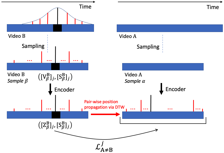
Figure 2: Illustration of pair-wise position propagation, showing the loss computation for the $j$th frame in the $\beta$ sample of video $\mathrm{B}$. We first calculate the Gaussian distribution of timestamp distances, centered around this frame. Afterwards, we propagate this distribution from video $\mathrm{B}$ to video $\mathrm{A}$ and minimize the KL-divergence between that distribution and the embedding similarity one.

3.4 Better Alignment via SoftDTW

The pair-wise position propagation as described above is effective only when the features used are representative enough. To improve this alignment during training, we suggest to also optimize the smooth DTW (SoftDTW) distance [23]. This is defined as follows,

$$r^{\gamma}(i,j)=D(i,j)+\text{min}^{\gamma}\{r^{\gamma}(i-1,j),r^{\gamma}(i,j-1),r^{\gamma}(i-1,j-1)\},$$ (10)

The term $r^{\gamma}(i,j)$ holds the soft-DTW distance up to frames $i$ and $j$ in the two videos, respectively. The expression $\text{min}^{\gamma}$ is a smooth (and therefore differentiable) version of the min function, defined as:

$$\text{min}^{\gamma}\{a_{1},a_{2},\ldots,a_{n}\}=-\gamma\log\sum_{i=1}^{n}e^{\frac{-a_{i}}{\gamma}}.$$ (11)

Note that $\text{min}^{\gamma}$ converges to the discrete $\min$ operator as $\gamma$ approaches zero. Therefore, when $\gamma$ is near zero, the smooth DTW distance will produce results that are similar to those of the discrete DTW.

Armed with the SoftDTW, given a single pair of videos with their randomly chosen indices, $(Z^{\mathrm{A}}_{\alpha},S^{\mathrm{A}}_{\alpha},Z^{\mathrm{B}}_{\beta},S^{\mathrm{B}}_{\beta})$, we optimize the following objective function:

$$\mathcal{L}_{\textbf{LRProp}}(Z^{\mathrm{A}}_{\alpha},S^{\mathrm{A}}_{\alpha},Z^{\mathrm{B}}_{\beta},S^{\mathrm{B}}_{\beta})=\delta_{\mathrm{A}\mathrm{B}}\cdot\mathcal{L}_{\text{Same}}+(1-\delta_{\mathrm{A}\mathrm{B}})\cdot(\lambda_{1}\cdot\mathcal{L}_{\text{Prop.}}+\lambda_{2}\cdot\mathcal{L}_{\text{Sdtw}}).$$ (12)

Here, $\delta_{\mathrm{A}\mathrm{B}}$ is the Kronecker delta, which is 1 if $\mathrm{A}=\mathrm{B}$ and 0 otherwise. $\mathcal{L}_{\text{Sdtw}}\equiv\mathcal{L}_{\text{Sdtw}}(Z^{\mathrm{A}}_{\alpha},Z^{\mathrm{B}}_{\beta})$ is the smooth DTW distance between the two videos, which is computed using the embedding vectors $Z^{\mathrm{A}}_{\alpha}$ and $Z^{\mathrm{B}}_{\beta}$ via Equation (10). $\lambda_{1}$ and $\lambda_{2}$ are hyper-parameters that control the relative importance of the different terms in this objective function. For further implementation details and hyper-parameters, see Appendix A.2.

4 Empirical Study

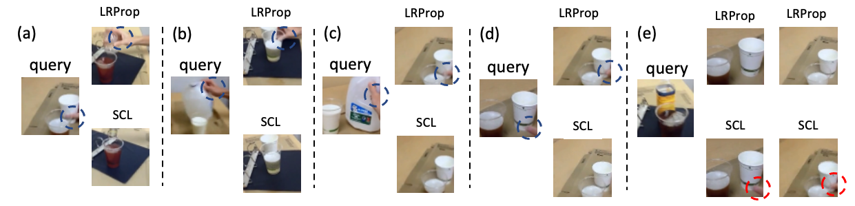
Figure 3: An example of aligned frames (Pouring dataset) using the DTW algorithm. In (a), (b), (c), and (d), LRProp is better at capturing the specific action of placing the bottle/cup, as indicated by the blue circles; in contrast, in SCL, the human hand is missing in the aligned frame. In (e), the query frame shows the end of the pouring action. Two aligned video results are shown; while LRProp provides a successful match, SCL features are inferior - observe the human hand still present in the frames, as indicated by the red circles.

In this section, we evaluate the performance of LRProp on two datasets using various evaluation metrics.

4.1 Datasets

The PennAction dataset [28] includes videos of humans performing various sports and exercise activities. We use 13 of these actions, following TCC [15]. The dataset includes a total of 1140 videos for training and 966 for testing, with each action set containing 40-134 train videos and 42-116 test videos. For evaluation, we obtain per-frame labels from LAV [18]. These videos contain 18 to 663 frames.

Pouring dataset [27]. This dataset contain videos showing the process of a hand pouring a liquid from one object to another. The phase labels, based on the TCC [15], consist of five classes. Following TCC, we use 70 videos for training and 14 for testing. These videos contain 186 to 797 frames.

4.2 Evaluation Metrics

We use the following metrics to evaluate the frame-wise trained representations:

Phase Classification Accuracy [15] is a metric that measures the per-frame accuracy of Phase Classification. To calculate this metric, we first extract features from the frames in the training and test data. Then, we train a support vector machine (SVM) [42] classifier on the phase labels for the training data, using the extracted features as input. The classifier is then used to predict the phase labels for each frame in the test data. The Phase Classification Accuracy is calculated as the proportion of correctly predicted labels, and is reported for different percentages of the SVM training set, in order to evaluate the representativeness of the learned features.

Table 1: Comparison with state-of-the-art methods on Pouring using various evaluation metrics: Phase Classification@% (Classification@%), Phase Progression (Progress), Kendall’s Tau ($\tau$), Average Precision@K (AP@K), DTW Accuracy (DTW A). Best method is in bold, second best in underlined. Our proposed technique (LRProp) dominates all other methods.

Method	$\tau$	Progress	AP@			Classification@				DTW A
			K=5	K=10	K=15	10	25	50	100
SCL	99.2	93.5	90.04†	89.69†	88.92†	85.78†	87.14†	89.45†	93.73	84.68†
SAL	79.61	77.28	84.05	83.77	83.79	87.63	-	87.58	88.81	-
TCN	85.12	80.44	83.56	83.31	83.01	89.67	-	87.32	89.53	-
TCC	86.36	83.73	87.16	86.68	86.54	90.65	-	91.11	91.53	-
LAV	85.61	80.54	89.13	89.13	89.22	91.61	-	92.82	92.84	-
VAVA	87.55	83.61	-	-	-	91.65	-	91.79	92.84	-
LRProp	99.46	94.09	92.41	90.33	90.86	92.7	93.88	94.44	94.36	90.22

Phase Progression [15] evaluates the accuracy of the embeddings in representing the advancement of a process or action. To compute this metric, we establish a rough estimate of the progress within a phase by calculating the difference in timestamps between a specific frame and key events, and then normalizing this difference by the total number of frames in the video. This measure is used as the target for a linear regression model, which is trained on the frame-wise embeddings. The Phase Progression metric is then calculated as the average R-squared measure (coefficient of determination) of the regression model on the test data. This metric captures how well the embeddings capture the relative progression of the phase within a video.

Average Precision@K [18] is a metric used to evaluate the accuracy of fine-grained frame retrieval, where K is the number of retrieved frames. To calculate this metric, we identify the K nearest frames (using KNN) to a given query frame, based on the frame-wise embeddings, and calculate the Average Precision, i.e., the average proportion of retrieved frames that have the same phase label as the query one. This metric is calculated for different values of K, to assess the performance of the frame-wise embeddings at different retrieval sizes. No additional training or fine-tuning is needed for calculating this metric.

Kendall’s Tau [15] is a correlation coefficient that evaluates the temporal alignment of two sequences. Unlike the other metrics discussed above, Kendall’s Tau does not require additional labels for evaluation. To calculate this metric, we first sample pairs of frames ($u_{i},u_{j}$) from the first video, which has $n$ frames, and retrieve the corresponding nearest neighbors (in the feature space), ($v_{p},v_{q}$), in the second video. This quadruplet of frame indices ($i,j,p,q$) is considered concordant if $i<j$ and $p<q$ or $i>j$ and $p>q$. Otherwise, it is considered discordant. Kendall’s Tau is then calculated as the ratio of concordant pairs to the total number of pairs, which captures how well the two sequences are aligned in time. More specifically, it is defined over all pairs of frames in the first video as: $\tau=(\text{no. of concordant pairs - no. of discordant pairs})/{n\choose 2}$. Kendall’s Tau is a measure of the alignment between two sequences in time, where a value of $1$ indicates perfect alignment and a value of $-1$ indicates that the sequences are aligned in the reverse order. One limitation of this metric is that it assumes that there are no repetitive frames in a video. We average this metric across all video pairs in the validation set.

DTW Accuracy is the ultimate metric that measures the ability of the frame-wise embeddings to capture both the phase labels and the Phase Progression of actions or processes in videos. To calculate this metric, we first apply the dynamic time warping (DTW) algorithm to a pair of videos, using the frame-wise embeddings as input. This produces a sequence of connections between corresponding frames in the two videos. The DTW Accuracy is then calculated as the proportion of connections that connect frames with the same phase label. By definition, DTW does not allow for discordant indices, and it’s accuracy metric is sensitive to both the ability of the embeddings to predict the phase labels and the ability to capture the Phase Progression. Overall, DTW Accuracy is a useful metric for evaluating the effectiveness of frame-wise embeddings at capturing the temporal structure of actions or processes in videos. We evaluate this metric on all pairs of videos in the validation set, and take the average as the final result.

Following the work in [18, 15, 18, 16], we use the first four metrics above to evaluate the effectiveness of frame-wise embeddings at capturing the temporal structure of actions or processes in videos. In addition, we propose to use the last metric (DTW Accuracy) in order to evaluate the suitability of the learned features for video alignment.

4.3 Comparison to State-of-the-Art

Table 2: Comparison with state-of-the-art methods on PennAction using various evaluation metrics. Best method is in bold and second best is underlined. LRProp outperforms all previous methods.

Method	$\tau$	Progress	AP@			Classification@
			K=5	K=10	K=15	10	50	75	100
SCL	98.5	91.8	92.28	92.1	91.82	-	-	-	93.07
SAL	76.12	69.6	-	-	-	74.87	78.26	-	79.96
TCN	81.2	72.17	77.84	77.51	77.28	81.99	83.67	-	84.04
TCC	81.35	73.53	76.74	76.27	75.88	81.26	83.35	-	84.45
LAV	80.5	66.13	79.13	79.98	78.9	83.56	83.95	-	84.25
VAVA	80.53	70.91	-	-	-	83.89	84.23	-	84.48
LRProp	99.09	93.03	92.46	92.2	92.03	91.9	92.96	93.17	93.25

Pouring Dataset. In Table 1 we compare our method with state-of-the-art methods on the task of Pouring. The best method for each metric is shown in bold, and the second best is underlined. Our proposed method outperforms all previous work on this dataset, with SCL performing the second best overall. As not all of our proposed metrics were reported in their original paper, we reproduced their results using their Github repository for a fair comparison with our results – these are marked by a ^†.

Our method demonstrates superiority over all other methods in all tasks. In particular, with our approach we achieve a Phase Classification Accuracy of $93.88$% by using only $25\%$ of the available labels, surpassing all other methods, even if they use 100% of the labels. Additionally, our method excels at identifying frames with similar semantics from other videos, as demonstrated by an improvement of almost $2.5\%$ in the Average Precision@K (AP@) column. We also see significant gains in Kendall’s tau and Phase progression metrics compared to SCL, which has already shown a phenomenal improvement of more than $10\%$ over all previous methods. Finally, the DTW Accuracy metric, which measures both Phase Classification and Phase Progression, shows a striking improvement of almost $6\%$ over the state-of-the-art, indicating that our proposed approach is highly effective for video alignment. This is also supported by Figure 3, which demonstrates the superior performance of LRProp compared to SCL in the alignment task: when given a query frame, LRProp is able to capture fine-grained actions more effectively. For further demonstration of LRProp on video alignment, see Figure 1, and the supplementary material.

Table 3: An ablation study of $\mathcal{L}_{\text{Prop.}}$ and $\mathcal{L}_{\text{Sdtw}}$ using various evaluation metrics. Best result in each column is in bold. Our suggested method is in the bottom row.

$\mathcal{L}_{\text{Same}}$	$\mathcal{L}_{\text{Prop.}}$	$\mathcal{L}_{\text{Sdtw}}$	$\tau$	Progress	AP@						Classification@						DTW A
					K=1	K=5	K=10	K=15	K=20	K=25	5	10	25	50	75	100
✓	✓		98.97	92.58	92.74	90.4	88.68	87.49	86.64	85.94	81.99	83.99	85.08	87	86.62	86.42	81.38
✓		✓	99.52	92.25	93.45	90.38	89.02	88.26	87.55	86.69	86.66	87.66	88.61	89.75	89.69	89.69	85
✓	✓	✓	99.46	94.09	94.09	92.41	91.66	90.86	90.45	90.07	91.8	92.7	93.88	94.44	94.46	94.36	90.22

PennAction Dataset. As shown in Table 2, our proposed method demonstrates superior performance in comparison to all other state-of-the-art approaches on the PennAction dataset. Utilizing a weakly-supervised approach specialized for alignment, we follow the approach of [15] and train a separate model for each of the 13 action classes in this dataset. The results shown in the table are the average across all 13 actions; for a more detailed breakdown of results see Appendix A.1, Table 4.

Our method consistently outperforms all prior work, as highlighted in bold, with SCL performing the second best overall. It is important to note, however, that SCL trained a single model for all 13 action classes (the authors did not report results for each class individually), whereas our method utilizes individualized models for each class. Furthermore, our method achieves an accuracy of $93.17\%$ using only 75% of available labels, surpassing all baselines in Phase Classification (even if they use all the labels). Additionally, we achieve more than a 1% improvement in the Phase Progression metric. This suggests that our method produces highly reliable features for video alignment and fine-grained retrieval, as supported by the small but consistent improvement in Kendall’s tau and Average Precision@K metrics. As we did not re-train SCL on this dataset, we do not report the DTW Accuracy in the table. LRProp achieves an impressive average DTW Accuracy of $90.15$%.

4.4 Ablation Study

SoftDTW and pair-wise position propagation: Is it a winning combination? We now turn to address this question by assessing the performance of these two loss terms, $\mathcal{L}_{\text{Prop.}}$ and $\mathcal{L}_{\text{Sdtw}}$, and their contribution on the pouring dataset. We measure the Phase Classification Accuracy for a more diverse set of label portions, and similarly, we measure the Average Precision accuracy for a larger range of K values. We also measure the Phase Progression, Kendall’s Tau and DTW Accuracy as in previous sections. The results are depicted in Table 3.

As can be seen, our design choices consistently improve across all evaluation metrics, with the exception of Kendall’s Tau, which is already close to saturation. We observe that the first and second rows of Table 3 have similar results in the Kendall’s Tau, Phase Progression, and Average Precision@K metrics. This suggests that the combination of $\mathcal{L}_{\text{Prop.}}$ and $\mathcal{L}_{\text{Sdtw}}$ is responsible for the improvement, rather than either one alone. Additionally, LRProp shows an average improvement of around 5% in the Phase Classification Accuracy metric for any choice of label percentage. Also, the striking improvement in the DTW Accuracy metric when using both $\mathcal{L}_{\text{Prop.}}$ and $\mathcal{L}_{\text{Sdtw}}$ is particularly noteworthy, as it suggests that the combined loss function is able to produce features that are highly effective for video alignment.

5 Conclusions

In this paper we introduce LRProp, a powerful method for extracting frame-level features that are particularly effective for aligning videos. Our approach involves using the dynamic time-warping (DTW) algorithm for establishing a prior distribution between frames from different videos based on their alignment path. In multiple experiments and commonly used metrics, we demonstrate that our method significantly outperforms various baselines in learning feature representations. We also evaluate DTW video alignment performance using the learned features and achieve a striking improvement of more than 5% compared to the previous state-of-the-art.

A potential area for future research is to adapt our method to work with videos that may contain outlier frames, by identifying and extracting them from the learning/inference processes. This may enable more robust features and better overall alignment between videos. Another challenging task refers to much longer videos, for which current solutions may face a severe memory and computational barriers.

To conclude, our results demonstrate that the proposed approach is highly effective at learning better frame-wise feature representations for videos. The use of pair-wise position propagation, combined with the SoftDTW, to relate frames between different videos is a particularly promising direction, as we demonstrate its potential to significantly improve the task of video alignment.

Appendix A Appendix

A.1 PennAction Breakdown

In this section, we present a detailed breakdown of LRProp performance on each action in the PennAction dataset. The results are summarized in Table 4.

Dataset	$\tau$	Progress		AP@						Classification@						DTW-A
			K=1	K=5	K=10	K=15	K=20	K=25	K=30	5	10	25	50	75	100
squat	99.58	97.08	90.9	90.73	90.22	90.11	89.95	89.83	89.74	91.19	90.43	91	91.07	91	91.57	87.4
pushup	99.08	92.7	92.58	92.53	92.39	92.32	92.2	92.12	92.02	90.77	89.27	91.86	93.17	93.25	93.19	92.35
tennis serve	98.66	95.54	90.05	89.44	89.2	89.03	88.76	88.58	88.47	89.4	91.31	91.52	91.17	91.74	91.69	87.85
tennis forhand	98.85	88.28	92.14	91.03	90.89	90.61	90.47	90.36	90.3	92.53	92.44	93.14	92.68	93.14	93.08	89.66
situp	99.33	95.39	96.83	96.81	96.7	96.63	96.51	96.41	96.4	96.81	96.72	97.04	96.97	97.08	97.08	95.74
pullup	99.23	96.8	96.73	96.52	96.46	96.39	96.33	96.23	96.18	96.4	96.34	95.66	95.54	96.13	96.27	95.25
jumping jacks	98.63	97.02	91.91	91.84	91.74	91.67	91.44	91.03	90.68	92.11	93.41	93.58	93.58	93.7	93.76	90.08
golf swing	98.92	98.19	95.02	95.3	94.98	94.64	94.46	94.26	94.14	94.92	94.92	94.97	95.28	95.37	95.4	92.69
bowl	98.84	76.21	92.33	90.65	89.73	89.13	88.56	88.22	87.85	84.57	85.02	84.53	84.9	85.25	85.68	83.88
benchpress	99.32	95.14	94.33	93.96	93.9	93.75	93.65	93.55	93.49	91.38	93.81	94.98	95.11	95.19	95.33	92.57
baseball swing	99.2	94.9	91.61	92.11	91.87	91.88	91.78	91.63	91.49	97.05	89.59	92.49	93.03	93.19	93.11	90.07
baseball pitch	99.35	98.05	92.92	92.91	92.73	92.59	92.55	92.43	92.32	92.18	93.11	94.62	94.94	95.18	95.29	90.93
clean and jerk	99.2	87.64	88.67	88.24	87.84	87.66	87.5	87.33	87.2	87.89	88.62	90.31	91.14	90.99	90.8	83.59

Table 4: PennAction breakdown. A breakdown of the performance of LRProp on each of the actions contained in the PennAction dataset, using various evaluation metrics: Phase Classification@% (Classification@%), Phase Progression (Progress), Kendall’s Tau ($\tau$), Average Precision@K (AP@K) and DTW Accuracy (DTW A).

A.2 Implementation Details

In our model, we use a ResNet-50 [43] pretrained by BYOL [44] as a frame-wise spatial encoder. We use a 7-layer Transformer encoder [24] with a hidden size of 256 and 8 heads to model temporal context. We set $\sigma^{2}=10$, recall Equations (2), (7), and $\tau=0.1$, recall Equation (1). We use the Adam optimizer with a learning rate of $10^{-4}$ and a weight decay of $10^{-5}$, and we apply a cosine decay schedule without restarts [45] to the learning rate. We fix a batch size of 2, and train for 300 epochs all considered datasets. We use the same spatial augmentations and temporal sampling technique as in [33, 16]. The number of sampled frames, $T$, and the regularization parameters, $\lambda_{1},\lambda_{2}$, recall Equation (12), are given in Table 5.

Dataset	Action class	T	$\lambda_{1}$	$\lambda_{2}$
PennAction	jumping jacks	20	0.01	0.4
	tennis serve	40		0.003
	tennis forhand
	baseball swing			0.001
	bowl	60
	situp	80		0.4
	benchpress
	baseball pitch
	golf swing			1.6
	pushup
	squat			0.8
	pullup
	clean and jerk
Pouring	-	240

Table 5: Hyper-parameters of LRProp regarding each dataset.

References

- [1] Kim D, Cho D, Kweon IS. Self-supervised video representation learning with space-time cubic puzzles. In: Proceedings of the AAAI conference on artificial intelligence. vol. 33; 2019. p. 8545-52.
- [2] Wang L, Guo Y, Liu L, Lin Z, Deng X, An W. Deep video super-resolution using HR optical flow estimation. IEEE Transactions on Image Processing. 2020;29:4323-36.
- [3] Khan Z, Jawahar CV, Tapaswi M. Grounded Video Situation Recognition. In: Oh AH, Agarwal A, Belgrave D, Cho K, editors. Advances in Neural Information Processing Systems; 2022. .
- [4] Hao Y, Wang S, Cao P, Gao X, Xu T, Wu J, et al. Attention in Attention: Modeling Context Correlation for Efficient Video Classification. IEEE Transactions on Circuits and Systems for Video Technology. 2022.
- [5] Zeng R, Huang W, Tan M, Rong Y, Zhao P, Huang J, et al. Graph convolutional networks for temporal action localization. In: Proceedings of the IEEE/CVF International Conference on Computer Vision; 2019. p. 7094-103.
- [6] Wang X, Xiong X, Neumann M, Piergiovanni A, Ryoo MS, Angelova A, et al. Attentionnas: Spatiotemporal attention cell search for video classification. In: European Conference on Computer Vision. Springer; 2020. p. 449-65.
- [7] Lei J, Berg TL, Bansal M. Detecting Moments and Highlights in Videos via Natural Language Queries. Advances in Neural Information Processing Systems. 2021;34:11846-58.
- [8] Zhai J, Yao X, Dong G, Jiang Q, Zhang Y. 3D dual-stream convolutional neural networks with simple recurrent unit network: A new framework for action recognition. In: 2022 4th International Conference on Communications, Information System and Computer Engineering (CISCE). IEEE; 2022. p. 509-15.
- [9] Han Y, Tan S. TwinLSTM: Two-channel LSTM Network for Online Action Detection. In: 2022 26th International Conference on Pattern Recognition (ICPR). IEEE; 2022. p. 3310-7.
- [10] Pan B, Cai H, Huang DA, Lee KH, Gaidon A, Adeli E, et al. Spatio-temporal graph for video captioning with knowledge distillation. In: Proceedings of the IEEE/CVF Conference on Computer Vision and Pattern Recognition; 2020. p. 10870-9.
- [11] Qiao M, Yuan T. Action Recognition based on Video Spatio-Temporal Transformer. In: 2022 IEEE International Conference on Artificial Intelligence and Computer Applications (ICAICA). IEEE; 2022. p. 477-81.
- [12] Chang Z, Zhang X, Wang S, Ma S, Gao W. STRPM: A Spatiotemporal Residual Predictive Model for High-Resolution Video Prediction. In: Proceedings of the IEEE/CVF Conference on Computer Vision and Pattern Recognition; 2022. p. 13946-55.
- [13] Wu B, Nair S, Martin-Martin R, Fei-Fei L, Finn C. Greedy hierarchical variational autoencoders for large-scale video prediction. In: Proceedings of the IEEE/CVF Conference on Computer Vision and Pattern Recognition; 2021. p. 2318-28.
- [14] Misra I, Zitnick CL, Hebert M. Shuffle and learn: unsupervised learning using temporal order verification. In: European conference on computer vision. Springer; 2016. p. 527-44.
- [15] Dwibedi D, Aytar Y, Tompson J, Sermanet P, Zisserman A. Temporal cycle-consistency learning. In: Proceedings of the IEEE/CVF conference on computer vision and pattern recognition; 2019. p. 1801-10.
- [16] Chen M, Wei F, Li C, Cai D. Frame-wise Action Representations for Long Videos via Sequence Contrastive Learning. In: Proceedings of the IEEE/CVF Conference on Computer Vision and Pattern Recognition; 2022. p. 13801-10.
- [17] Purushwalkam S, Ye T, Gupta S, Gupta A. Aligning videos in space and time. In: European Conference on Computer Vision. Springer; 2020. p. 262-78.
- [18] Haresh S, Kumar S, Coskun H, Syed SN, Konin A, Zia Z, et al. Learning by aligning videos in time. In: Proceedings of the IEEE/CVF Conference on Computer Vision and Pattern Recognition; 2021. p. 5548-58.
- [19] Berndt DJ, Clifford J. Using dynamic time warping to find patterns in time series. In: KDD workshop. vol. 10. Seattle, WA, USA:; 1994. p. 359-70.
- [20] Tran D, Bourdev L, Fergus R, Torresani L, Paluri M. Learning spatiotemporal features with 3d convolutional networks. In: Proceedings of the IEEE international conference on computer vision; 2015. p. 4489-97.
- [21] Carreira J, Zisserman A. Quo vadis, action recognition? a new model and the kinetics dataset. In: proceedings of the IEEE Conference on Computer Vision and Pattern Recognition; 2017. p. 6299-308.
- [22] Farha YA, Gall J. Ms-tcn: Multi-stage temporal convolutional network for action segmentation. In: Proceedings of the IEEE/CVF Conference on Computer Vision and Pattern Recognition; 2019. p. 3575-84.
- [23] Cuturi M, Blondel M. Soft-dtw: a differentiable loss function for time-series. In: International conference on machine learning. PMLR; 2017. p. 894-903.
- [24] Vaswani A, Shazeer N, Parmar N, Uszkoreit J, Jones L, Gomez AN, et al. Attention is all you need. Advances in neural information processing systems. 2017;30.
- [25] Arnab A, Dehghani M, Heigold G, Sun C, Lučić M, Schmid C. Vivit: A video vision transformer. In: Proceedings of the IEEE/CVF International Conference on Computer Vision; 2021. p. 6836-46.
- [26] Neimark D, Bar O, Zohar M, Asselmann D. Video transformer network. In: Proceedings of the IEEE/CVF International Conference on Computer Vision; 2021. p. 3163-72.
- [27] Sermanet P, Lynch C, Chebotar Y, Hsu J, Jang E, Schaal S, et al. Time-contrastive networks: Self-supervised learning from video. In: 2018 IEEE international conference on robotics and automation (ICRA). IEEE; 2018. p. 1134-41.
- [28] Zhang W, Zhu M, Derpanis KG. From actemes to action: A strongly-supervised representation for detailed action understanding. In: Proceedings of the IEEE international conference on computer vision; 2013. p. 2248-55.
- [29] Doersch C, Gupta A, Efros AA. Unsupervised visual representation learning by context prediction. In: Proceedings of the IEEE international conference on computer vision; 2015. p. 1422-30.
- [30] Noroozi M, Favaro P. Unsupervised learning of visual representations by solving jigsaw puzzles. In: European conference on computer vision. Springer; 2016. p. 69-84.
- [31] Zhang R, Isola P, Efros AA. Colorful image colorization. In: European conference on computer vision. Springer; 2016. p. 649-66.
- [32] Chen T, Zhai X, Ritter M, Lucic M, Houlsby N. Self-supervised gans via auxiliary rotation loss. In: Proceedings of the IEEE/CVF conference on computer vision and pattern recognition; 2019. p. 12154-63.
- [33] Chen T, Kornblith S, Norouzi M, Hinton G. A simple framework for contrastive learning of visual representations. In: International conference on machine learning. PMLR; 2020. p. 1597-607.
- [34] Chen T, Kornblith S, Swersky K, Norouzi M, Hinton GE. Big self-supervised models are strong semi-supervised learners. Advances in neural information processing systems. 2020;33:22243-55.
- [35] Caron M, Touvron H, Misra I, Jégou H, Mairal J, Bojanowski P, et al. Emerging properties in self-supervised vision transformers. In: Proceedings of the IEEE/CVF International Conference on Computer Vision; 2021. p. 9650-60.
- [36] Srivastava N, Mansimov E, Salakhudinov R. Unsupervised learning of video representations using lstms. In: International conference on machine learning. PMLR; 2015. p. 843-52.
- [37] Vondrick C, Pirsiavash H, Torralba A. Generating videos with scene dynamics. Advances in neural information processing systems. 2016;29.
- [38] Yadav R, Sardana A, Namboodiri VP, Hegde RM. Learning to Predict Speech in Silent Videos Via Audiovisual Analogy. In: ICASSP 2022-2022 IEEE International Conference on Acoustics, Speech and Signal Processing (ICASSP). IEEE; 2022. p. 8042-6.
- [39] Liu W, Tekin B, Coskun H, Vineet V, Fua P, Pollefeys M. Learning to align sequential actions in the wild. In: Proceedings of the IEEE/CVF Conference on Computer Vision and Pattern Recognition; 2022. p. 2181-91.
- [40] Chang CY, Huang DA, Sui Y, Fei-Fei L, Niebles JC. D3tw: Discriminative differentiable dynamic time warping for weakly supervised action alignment and segmentation. In: Proceedings of the IEEE/CVF Conference on Computer Vision and Pattern Recognition; 2019. p. 3546-55.
- [41] Hadji I, Derpanis KG, Jepson AD. Representation learning via global temporal alignment and cycle-consistency. In: Proceedings of the IEEE/CVF Conference on Computer Vision and Pattern Recognition; 2021. p. 11068-77.
- [42] Hearst MA, Dumais ST, Osuna E, Platt J, Scholkopf B. Support vector machines. IEEE Intelligent Systems and their applications. 1998;13(4):18-28.
- [43] He K, Zhang X, Ren S, Sun J. Deep residual learning for image recognition. In: Proceedings of the IEEE conference on computer vision and pattern recognition; 2016. p. 770-8.
- [44] Grill JB, Strub F, Altché F, Tallec C, Richemond P, Buchatskaya E, et al. Bootstrap your own latent-a new approach to self-supervised learning. Advances in neural information processing systems. 2020;33:21271-84.
- [45] Loshchilov I, Hutter F. Sgdr: Stochastic gradient descent with warm restarts. arXiv preprint arXiv:160803983. 2016.