Approximately Optimal Core Shapes for Tensor Decompositions

Abstract

This work studies the combinatorial optimization problem of finding an optimal core tensor shape, also called multilinear rank, for a size-constrained Tucker decomposition. We give an algorithm with provable approximation guarantees for its reconstruction error via connections to higher-order singular values. Specifically, we introduce a novel Tucker packing problem, which we prove is NP-hard, and give a polynomial-time approximation scheme based on a reduction to the 2-dimensional knapsack problem with a matroid constraint. We also generalize our techniques to tree tensor network decompositions. We implement our algorithm using an integer programming solver, and show that its solution quality is competitive with (and sometimes better than) the greedy algorithm that uses the true Tucker decomposition loss at each step, while also running up to 1000x faster.

1 Introduction

Low-rank tensor decomposition is a powerful tool in the modern machine learning toolbox. Like low-rank matrix factorization, it has countless applications in scientific computing, data mining, and signal processing (Kolda & Bader, 2009; Sidiropoulos et al., 2017), e.g., anomaly detection in data streams (Jang & Kang, 2021) and compressing convolutional neural networks on mobile devices for faster inference while reducing power consumption (Kim et al., 2016).

The most widely used tensor decompositions are the canonical polyadic (CP) decomposition, Tucker decomposition, and tensor-train decomposition (Oseledets, 2011)—the last two being instances of tree tensor networks (Krämer, 2020). CP decomposition factors a tensor into the sum of $r$ rank-one tensors. Tucker decomposition, however, specifies the rank $R_{n}$ in each dimension $n$ and relies on a core tensor $\bm{\mathscr{G}}\in\mathbb{R}^{R_{1}\times\dots\times R_{N}}$ for reconstructing the decomposition. The notion of multilinear rank $\mathbf{r}=(R_{1},\dots,R_{N})$ puts practitioners in a challenging spot because the set of feasible core shapes can be exponentially large. Furthermore, searching in this state space can be prohibitively expensive because evaluating the true quality of a core shape requires computing a Tucker decomposition, which for large tensors can take hours and consume hundreds of GB of RAM. For example, in the MATLAB Tensor Toolbox (Bader & Kolda, 2022), we need to specify the core shape parameter ranks in advance before computing a size-constrained Tucker decomposition.

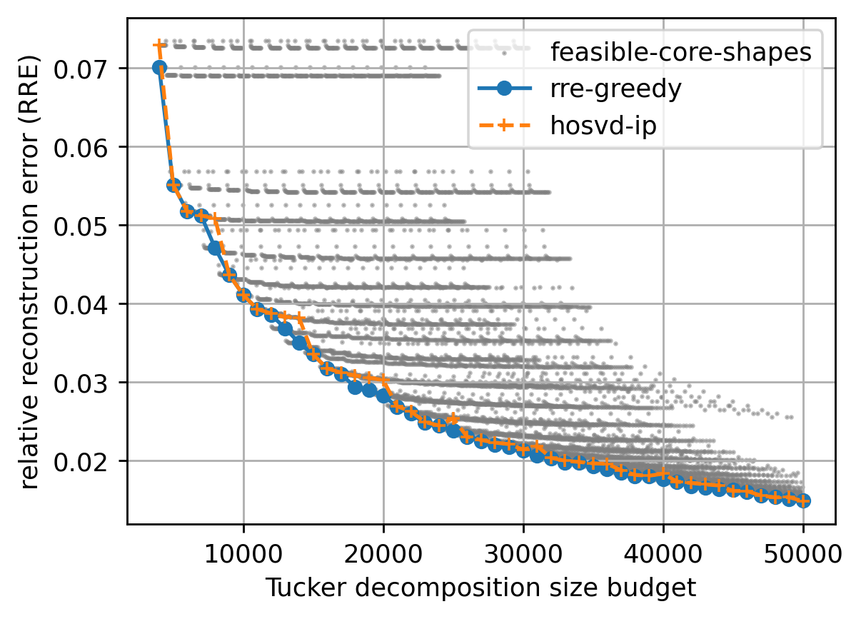
Figure 1: Pareto frontier of core shapes $\mathbf{r}\in[20]^{3}$ for hyperspectral tensor $\bm{\mathscr{X}}\in\mathbb{R}^{1024\times 1344\times 33}$. Plots the RRE, i.e., $L(\bm{\mathscr{X}},\mathbf{r})/\lVert\bm{\mathscr{X}}\rVert_{\textnormal{F}}^{2}$, as a function of compression rate. RRE-greedy builds core shapes by computing Tucker decompositions at each step. HOSVD-IP is Algorithm 2 with integer programming, which builds core shapes via a surrogate packing problem on higher-order singular values.

In practice, the most popular Tucker decomposition algorithms are the $\mathbf{r}$-truncated higher-order singular value decomposition (HOSVD) in De Lathauwer et al. (2000a), sequentially truncated ST-HOSVD in Vannieuwenhoven et al. (2012), and higher-order orthogonal iteration (HOOI), which is a structured alternating least squares algorithm.

We explore the simple but fundamental discrete optimization problem for low-rank tensor decompositions:

If a Tucker decomposition of $\bm{\mathscr{X}}$ can use at most $c$ parameters, which core tensor shape minimizes the reconstruction error?

This is a multilinear generalization of the best rank-$r$ matrix approximation problem. While there are many parallels to low-rank matrix factorization, tensor rank-related problems can be thoroughly different and more challenging than their matrix counterparts. For example, computing the CP rank of a real-valued tensor is NP-hard  (Hillar & Lim, 2013).

1.1 Our contributions and techniques

We summarize the main contributions of this work below:

1. We formalize the core tensor shape problem for size-constrained Tucker decompositions and introduce the Tucker packing problem, which we prove is NP-hard. The approximation algorithms we develop build on a relationship between the optimal reconstruction error of a rank-$\mathbf{r}$ Tucker decomposition and a multi-dimensional tail sum of its higher-order singular values (De Lathauwer et al., 2000a; Hackbusch, 2019).

2. We design a polynomial-time approximation scheme (PTAS) for the surrogate Tucker packing problem (Theorem 4.6) by showing that it suffices to consider a small number of budget splits between the cost of the core tensor and the cost of the factor matrices. Each budget split subproblem reduces to a 2-dimensional knapsack problem with a partition matroid constraint after minor transformations. We solve these knapsack problems using the PTAS of Grandoni et al. (2014), or in practice with integer linear programming.

3. We extend our approach to tree tensor networks, which generalize the Tucker decomposition, tensor-train decomposition, and hierarchical Tucker decomposition. In doing so, we synthesize several works on tree tensors from the mathematics and physics communities, and give a succinct introduction for computer scientists.

4. Finally, we demonstrate the effectiveness of our Tucker packing-based core shape solvers on four real-world tensors. Our HOSVD-IP algorithm is competitive with (and sometimes outperforms) the greedy algorithm that uses the true RRE, while running up to 1000x faster.

1.2 Related works

Core shape constraints.

De Lathauwer et al. (2000b) introduced the problem of computing the best rank-$\mathbf{r}$ tensor approximation for a prespecified core shape $\mathbf{r}$, and demonstrated the benefit of initializing the decomposition with a truncated HOSVD and then running iterative methods such as HOOI. Eldén & Savas (2009); Ishteva et al. (2009, 2011, 2013); Eldén & Dehghan (2022) consider this problem for rank-$(r_{1},r_{2},r_{3})$ decompositions and develop a suite of advanced algorithms: a Newton method on Grassmannian manifolds, a trust-region method on Riemannian manifolds, Jacobi rotations for symmetric tensors, and a Krylov-type iterative method. All these works, however, are concerned with optimizing the tensor decomposition for a fixed core shape—not with optimizing the core tensor shape itself.

Ehrlacher et al. (2021) and Xiao & Yang (2021) recently explored rank-adaptive methods for HOOI that find minimal core shapes such that the Tucker decomposition achieves a target reconstruct error. They also leverage properties of the HOSVD, but they do not impose a hard constraint on the size of the returned Tucker decomposition. Hashemizadeh et al. (2020) generalized the RRE-greedy algorithm in Figure 1 to tensor networks for both rank and size constraints.

Low-rank tensor decomposition.

Song et al. (2019) gave polynomial-time $(1+\varepsilon)$-approximation algorithms for many types of low-rank tensor decompositions with respect to the Frobenius norm, including CP and Tucker decompositions. Frandsen & Ge (2022) showed that if a third-order tensor has an exact Tucker decomposition, then all local minima of an appropriately regularized loss landscape are globally optimal. Several works recently studied Tucker decomposition in streaming models (Traoré et al., 2019; Sun et al., 2020) and a sliding window model (Jang & Kang, 2021). Fast randomized low-rank tensor decomposition algorithms based on sketching have been proposed in Zhou et al. (2014); Cheng et al. (2016); Battaglino et al. (2018); Malik & Becker (2018); Che & Wei (2019); Ma & Solomonik (2021); Larsen & Kolda (2022); Fahrbach et al. (2022); Malik (2022).

2 Preliminaries

Notation.

The order of a tensor is its number of dimensions. We denote scalars by normal lowercase letters $x\in\mathbb{R}$, vectors by boldface lower letters $\mathbf{x}\in\mathbb{R}^{n}$, matrices by boldface uppercase letters $\mathbf{X}\in\mathbb{R}^{m\times n}$, and higher-order tensors by boldface script letters $\bm{\mathscr{X}}\in\mathbb{R}^{I_{1}\times\dots\times I_{N}}$. We use normal uppercase letters for the size of an index set, e.g., $[N]=\{1,2,\dots,N\}$. We denote the $i$-th entry of vector $\mathbf{x}$ by $x_{i}$, the $(i,j)$-th entry of matrix $\mathbf{X}$ by $x_{ij}$, and the $(i,j,k)$-th entry of a third-order tensor $\bm{\mathscr{X}}$ by $x_{ijk}$.

Tensor products.

The fibers of a tensor are the vectors we get by fixing all but one index. For example, if $\bm{\mathscr{X}}\in\mathbb{R}^{3}$, we denote the column, row, and tube fibers by $\mathbf{x}_{:jk}$, $\mathbf{x}_{i:k}$, and $\mathbf{x}_{ij:}$, respectively. The mode-$n$ unfolding of a tensor $\bm{\mathscr{X}}\in\mathbb{R}^{I_{1}\times\dots\times I_{N}}$ is the matrix $\mathbf{X}_{(n)}\in\mathbb{R}^{I_{n}\times(I_{1}\dots I_{n-1}I_{n+1}\dots I_{N})}$ that arranges the mode-$n$ fibers of $\bm{\mathscr{X}}$ as columns of $\mathbf{X}_{(n)}$ ordered lexicographically by index.

We denote the $n$-mode product of a tensor $\bm{\mathscr{X}}\in\mathbb{R}^{I_{1}\times\dots\times I_{N}}$ and matrix $\mathbf{A}\in\mathbb{R}^{J\times I_{N}}$ by $\bm{\mathscr{Y}}=\bm{\mathscr{X}}\times_{n}\mathbf{A}$, where $\bm{\mathscr{Y}}\in\mathbb{R}^{I_{1}\times\dots\times I_{n-1}\times J\times I_{n+1}\times\dots\times I_{N}}$. This operation multiplies each mode-$n$ fiber of $\bm{\mathscr{X}}$ by $\mathbf{A}$, and can be expressed element-wise as

$$(\bm{\mathscr{X}}\times_{n}\mathbf{A})_{i_{1}\dots i_{n-1}ji_{n+1}\dots i_{N}}=\sum_{i_{n}=1}^{I_{n}}x_{i_{1}i_{2}\dots i_{N}}a_{ji_{n}}.$$

The inner product of two tensors $\bm{\mathscr{X}},\bm{\mathscr{Y}}\in\mathbb{R}^{I_{1}\times\dots\times I_{N}}$ is the sum of the products of their entries:

$$\langle\bm{\mathscr{X}},\bm{\mathscr{Y}}\rangle=\sum_{i_{1}=1}^{I_{1}}\sum_{i_{2}=1}^{I_{2}}\dots\sum_{i_{N}=1}^{I_{N}}x_{i_{1}i_{2}\dots i_{N}}y_{i_{1}i_{2}\dots i_{N}}.$$

The Frobenius norm of a tensor $\bm{\mathscr{X}}$ is $\lVert\bm{\mathscr{X}}\rVert_{\textnormal{F}}=\sqrt{\langle\bm{\mathscr{X}},\bm{\mathscr{X}}\rangle}$.

Tucker decomposition.

The Tucker decomposition of a tensor $\bm{\mathscr{X}}\in\mathbb{R}^{I_{1}\times\dots\times I_{N}}$ decomposes $\bm{\mathscr{X}}$ into a core tensor $\bm{\mathscr{G}}\in\mathbb{R}^{R_{1}\times\dots\times R_{N}}$ and $N$ factor matrices $\mathbf{A}^{(n)}\in\mathbb{R}^{I_{n}\times R_{n}}$. We refer to $\mathbf{r}=(R_{1},\dots,R_{N})$ as the core shape, which is also called the multilinear rank or truncation of the decomposition. We denote the loss of an optimal rank-$\mathbf{r}$ Tucker decomposition by

$$L(\bm{\mathscr{X}},\mathbf{r})\operatorname*{\overset{def}{=}}\min_{\bm{\mathscr{G}}\in\mathbb{R}^{R_{1}\times\dots\times R_{N}}}\lVert\bm{\mathscr{X}}-\bm{\mathscr{G}}\times_{1}\mathbf{A}^{(1)}\times_{2}\dots\times_{N}\mathbf{A}^{(N)}\rVert_{\textnormal{F}}^{2}.$$

3 Reduction to HOSVD Tucker packing

3.1 Higher-order singular value decomposition

We start with a recap of the seminal work on higher-order singular value decompositions (HOSVD) by De Lathauwer, De Moor, and Vandewalle (2000a).

Theorem 3.1 (De Lathauwer et al. (2000a, Theorem 2)).

Any tensor $\bm{\mathscr{X}}\in\mathbb{R}^{I_{1}\times\cdots\times I_{N}}$ can be written as

$$\bm{\mathscr{X}}=\bm{\mathscr{S}}\times_{1}\mathbf{U}^{(1)}\times_{2}\cdots\times_{N}\mathbf{U}^{(N)},$$

where each $\mathbf{U}^{(n)}\in{\mathbb{R}}^{I_{n}\times I_{n}}$ is an orthogonal matrix and $\bm{\mathscr{S}}\in\mathbb{R}^{I_{1}\times\cdots\times I_{N}}$ is a tensor with subtensors $\bm{\mathscr{S}}_{i_{n}=\alpha}$, obtained by fixing the $n$-th index to $\alpha$, that have the properties:

1. all-orthogonality: for all possible values of $n$, $\alpha$ and $\beta$ subject to $\alpha\neq\beta$, two subtensors $\bm{\mathscr{S}}_{i_{n}=\alpha}$ and $\bm{\mathscr{S}}_{i_{n}=\beta}$ are orthgonal, i.e., $\left\langle\bm{\mathscr{S}}_{i_{n}=\alpha},\bm{\mathscr{S}}_{i_{n}=\beta}\right\rangle=0\text{~{}when~{}}\alpha\neq\beta;$

2. ordering: for all values of $n$, $\lVert\bm{\mathscr{S}}_{i_{n}=1}\rVert_{\textnormal{F}}\geq\lVert\bm{\mathscr{S}}_{i_{n}=2}\rVert_{\textnormal{F}}\geq\dots\geq\lVert\bm{\mathscr{S}}_{i_{n}=I_{n}}\rVert_{\textnormal{F}}\geq 0.$

Furthermore, the values $\lVert\bm{\mathscr{S}}_{i_{n}=i}\rVert_{\textnormal{F}}$, denoted by $\sigma_{i}^{(n)}$, are the singular values of the mode-$n$ unfolding $\mathbf{X}_{(n)}$, and the columns of $\mathbf{U}^{(n)}$ are the the left singular vectors.

Next, we present the TuckerHOSVD algorithm. This is a widely used initialization strategy when computing rank-$\mathbf{r}$ Tucker decompositions (Kolda & Bader, 2009), i.e., if the core shape $\mathbf{r}$ is predetermined.

Algorithm 1 TuckerHOSVD

Input: $\bm{\mathscr{X}}\in\mathbb{R}^{I_{1}\times\cdots\times I_{N}}$, core shape $\mathbf{r}=(R_{1},\dots,R_{N})$

1:  for $n=1$ to $N$ do

2:     $\mathbf{A}^{(n)}\leftarrow R_{n}\text{ top left singular vectors of }\mathbf{X}_{(n)}$

3:  end for

4:  $\bm{\mathscr{G}}\leftarrow\bm{\mathscr{X}}\times_{1}{\mathbf{A}^{(1)}}\times_{2}\dots\times_{N}{\mathbf{A}^{(N)}}$

5:  return $\bm{\mathscr{G}},\mathbf{A}^{(1)},\mathbf{A}^{(2)},\dots,\mathbf{A}^{(N)}$

The output of TuckerHOSVD has the following error guarantees (De Lathauwer et al., 2000a; Hackbusch, 2019). These bounds suggest a less expensive surrogate loss function to minimize instead when optimizing the core tensor shape subject to a Tucker decomposition size constraint. We give self-contained proofs of these results in Section A.1 that build on Theorem 3.1.

Theorem 3.2 (Property 10).

HOSVD; Hackbusch (2019, Theorem 10.2)] For any tensor $\bm{\mathscr{X}}\in\mathbb{R}^{I_{1}\times\dots\times I_{N}}$ and core shape $\mathbf{r}\in[I_{1}]\times\dots\times[I_{N}]$, let the output of $\textup{{TuckerHOSVD}}(\bm{\mathscr{X}},\mathbf{r})$ be $\bm{\mathscr{G}}\in\mathbb{R}^{R_{1}\times\dots\times R_{N}}$ and $\mathbf{A}^{(n)}\in\mathbb{R}^{I_{n}\times R_{n}}$, for each $n\in[N]$. If we let

$$\widehat{\bm{\mathscr{X}}}_{\textnormal{HOSVD}(\mathbf{r})}\operatorname*{\overset{def}{=}}\bm{\mathscr{G}}\times_{1}\mathbf{A}^{(1)}\times_{2}\dots\times_{N}\mathbf{A}^{(N)}$$ (1)

denote the reconstructed $\mathbf{r}$-truncated tensor, then

$$\lVert\bm{\mathscr{X}}-\widehat{\bm{\mathscr{X}}}_{\textnormal{HOSVD}(\mathbf{r})}\rVert_{\textnormal{F}}^{2} \leq\sum_{n=1}^{N}\sum_{i_{n}=R_{n}+1}^{I_{n}}\left(\sigma_{i_{n}}^{(n)}\right)^{2}$$

$$\leq N\cdot L(\bm{\mathscr{X}},\mathbf{r}).$$

Furthermore, we have $L(\bm{\mathscr{X}},\mathbf{r})\leq\lVert\bm{\mathscr{X}}-\widehat{\bm{\mathscr{X}}}_{\textnormal{HOSVD}(\mathbf{r})}\rVert_{\textnormal{F}}^{2}.$

Theorem 3.2 implies that the following function is a meaningful proxy for the reconstruction error of an optimal rank-$\mathbf{r}$ Tucker decomposition.

Definition 3.3.

Define the surrogate loss of core shape $\mathbf{r}$ as

$$\widetilde{L}(\bm{\mathscr{X}},\mathbf{r}) \operatorname*{\overset{def}{=}}\sum_{n=1}^{N}\sum_{i_{n}=R_{n}+1}^{I_{n}}\left(\sigma_{i_{n}}^{(n)}\right)^{2}.$$ (2)

To summarize so far, for any core shape $\mathbf{r}\in[I_{1}]\times\dots\times[I_{N}]$, we are guaranteed that $\nicefrac{{1}}{{N}}\cdot\widetilde{L}(\bm{\mathscr{X}},\mathbf{r})\leq L(\bm{\mathscr{X}},\mathbf{r})\leq\widetilde{L}(\bm{\mathscr{X}},\mathbf{r}).$ We refer the reader to Section A.2 for the full details.

3.2 Tucker packing problem

Next, observe that the sum of squared singular values across all mode-$n$ unfoldings of $\bm{\mathscr{X}}$ is

$$\sum_{n=1}^{N}\sum_{i_{n}=1}^{I_{n}}\left(\sigma_{i_{n}}^{(n)}\right)^{2}=\sum_{n=1}^{N}\lVert\mathbf{X}_{(n)}\rVert_{\textnormal{F}}^{2}=N\lVert\bm{\mathscr{X}}\rVert_{\textnormal{F}}^{2}.$$

This means we can solve a singular value packing problem instead by considering the complement of the surrogate loss. The following lemma is a wrapper for the truncated HOSVD error guarantees in Theorem 3.2.

Lemma 3.4.

For any tensor $\bm{\mathscr{X}}\in\mathbb{R}^{I_{1}\times\dots\times I_{N}}$ and budget $c\geq 1+\sum_{n=1}^{N}I_{n}$ for the size of the Tucker decomposition, let the set of feasible core shapes be

$$F=\left\{\mathbf{r}\in[I_{1}]\times\cdots\times[I_{N}]:\prod_{n=1}^{N}R_{n}+\sum_{n=1}^{N}I_{n}R_{n}\leq c\right\}.$$

Then, we have

$$\widetilde{\mathbf{r}}^{*}\operatorname*{\overset{def}{=}}\operatorname*{arg\,min}_{\mathbf{r}\in F}\widetilde{L}(\bm{\mathscr{X}},\mathbf{r})=\operatorname*{arg\,max}_{\mathbf{r}\in F}\sum_{n=1}^{N}\sum_{i_{n}=1}^{R_{n}}\left(\sigma_{i_{n}}^{(n)}\right)^{2}.$$

Further, if $\mathbf{r}^{*}\operatorname*{\overset{def}{=}}\operatorname*{arg\,min}_{\mathbf{r}\in F}L(\bm{\mathscr{X}},\mathbf{r})$ is an optimal budget-constrained core shape, then $L\left(\bm{\mathscr{X}},\widetilde{\mathbf{r}}^{*}\right)\leq N\cdot L\left(\bm{\mathscr{X}},\mathbf{r}^{*}\right).$

To find a core shape whose optimal Tucker decomposition approximates the optimal loss $L(\bm{\mathscr{X}},\mathbf{r}^{*})$ subject to a size constraint, we solve the maximization problem in Lemma 3.4. Optimizing this proxy objective is substantially less expensive than methods that rely on rank-$\mathbf{r}$ Tucker decomposition solvers as a subroutine. We formalize this idea by introducing the more general problem below.

Definition 3.5 (Tucker packing problem).

Given a shape $(I_{1},\dots,I_{N})\in\mathbb{Z}_{\geq 1}^{N}$, $N$ non-increasing sequences $\mathbf{a}^{(n)}\in\mathbb{R}_{\geq 0}^{I_{n}}$, and a budget $c\geq 1$, the Tucker packing problem asks to find a core shape $\mathbf{r}\in[I_{1}]\times\dots\times[I_{N}]$ that solves:

We also denote the objective by $f(\mathbf{r})\operatorname*{\overset{def}{=}}\sum_{n=1}^{N}\sum_{i_{n}=1}^{R_{n}}a_{i_{n}}^{(n)}.$

Theorem 3.6.

The Tucker packing problem is NP-hard.

We prove this result in Section A.3 with an intricate reduction from the EQUIPARTITION problem (see, e.g., Garey & Johnson (1979, SP12)).

NP-hardness motivates the need for efficient approximation algorithms. In Section 4, we develop a polynomial-time approximation scheme (PTAS) for the Tucker packing problem. We leave the existence of a fully-polynomial time approximation scheme (FPTAS) as a challenging open question for future works.

To conclude, since Tucker packing is the complement of surrogate loss minimization, we must quantify how a $(1-\varepsilon)$-approximation for the packing problem can affect the error incurred in the surrogate loss. We explain this in detail in Section A.4 and present the main idea below.

Lemma 3.7.

Let $\mathbf{r}\in[I_{1}]\times\dots\times[I_{N}]$ be any core shape that achieves a $(1-\varepsilon/N)$-approximation to the Tucker packing problem. Then, we have $\textnormal{RRE}(\bm{\mathscr{X}},\mathbf{r})\leq N\cdot\textnormal{RRE}(\bm{\mathscr{X}},\mathbf{r}^{*})+\varepsilon,$ where $\textnormal{RRE}(\bm{\mathscr{X}},\mathbf{r}):=L(\bm{\mathscr{X}},\mathbf{r})/\lVert\bm{\mathscr{X}}\rVert_{\textnormal{F}}^{2}$.

Remark 3.8.

We can obtain global approximation guarantees for Tucker decomposition reconstruction error by (1) finding an approximately optimal core shape, (2) running TuckerHOSVD to initialize the Tucker decomposition, and (3) using alternating least squares (ALS) to improve the tensor decomposition. This is analogous to how $k$-means++ enhances Lloyd’s algorithm (Arthur & Vassilvitskii, 2006).

4 Algorithm

4.1 Warm-up: Connections to multiple-choice knapsack

To start, consider a simplified version of the Tucker packing problem that only accounts for the size of the core tensor, i.e., the factor matrices do not use any of the budget. We show that after two simple transformations this new problem reduces to the multiple-choice knapsack problem, which is NP-hard (Pisinger, 1995) but has an FPTAS (Lawler, 1977).

Concretely, the optimization problem is

maximize $$\sum_{n=1}^{N}\sum_{i_{n}=1}^{R_{n}}a_{i_{n}}^{(n)}$$ (5)

subject to $$\prod_{n=1}^{N}R_{n}\leq c$$ (6)

Prefix sums transformation.

To get closer to a 0-1 knapsack problem, define new coefficients by taking the prefix sums of the $a_{i_{n}}^{(n)}$’s, for each $n\in[N]$ and $i_{n}\in[I_{n}]$:

$$p_{i_{n}}^{(n)}\operatorname*{\overset{def}{=}}\sum_{j_{n}=1}^{i_{n}}a_{j_{n}}^{(n)}.$$

This “core size-only” Tucker packing problem can be reformulated as the following integer program:

maximize $$\sum_{n=1}^{N}\sum_{i_{n}=1}^{I_{n}}p_{i_{n}}^{(n)}x_{i_{n}}^{(n)}$$

subject to $$\prod_{n=1}^{N}\sum_{i_{n}=1}^{I_{n}}i_{n}x_{i_{n}}^{(n)}\leq c$$ (7)

$$\sum_{i_{n}=1}^{I_{n}}x_{i_{n}}^{(n)}=1\hskip 28.45274pt\forall n\in[N]$$

$$x_{i_{n}}^{(n)}\in\{0,1\}\hskip 31.58257pt\forall n\in[N],i_{n}\in[I_{n}]$$

We optimize over $i_{n}$ instead of $R_{n}$ for notational brevity.

Log transformation.

Next, replace constraint (7) with the linear inequality

$$\sum_{n=1}^{N}\sum_{i_{n}=1}^{I_{n}}\log(i_{n})x_{i_{n}}^{(n)}\leq\log(c).$$

This substitution is valid because in any feasible solution, for each $n\in[N]$, exactly one of $x_{1}^{(n)},x_{2}^{(n)},\dots,x_{I_{n}}^{(n)}$ is equal to one and the rest are zero. Putting everything together, this core size-only Tucker packing problem is the following multiple-choice knapsack problem:

maximize $$\sum_{n=1}^{N}\sum_{i_{n}=1}^{I_{n}}p_{i_{n}}^{(n)}x_{i_{n}}^{(n)}$$ (8)

subject to $$\sum_{n=1}^{N}\sum_{i_{n}=1}^{I_{n}}\log(i_{n})x_{i_{n}}^{(n)}\leq\log(c)$$

$$\sum_{i_{n}=1}^{I_{n}}x_{i_{n}}^{(n)}=1\hskip 28.45274pt\forall n\in[N]$$

$$x_{i_{n}}^{(n)}\in\{0,1\}\hskip 31.58257pt\forall n\in[N],i_{n}\in[I_{n}]$$

Theorem 4.1 (Lawler 1977).

There exists an algorithm that computes a $(1-\varepsilon)$-approximation to problem (8) in time and space $O(N^{2}\varepsilon^{-1}\sum_{n=1}^{N}I_{n})$.

The FPTAS in Theorem 4.1 for multiple-choice knapsack uniformly downscales all coefficients $p_{i_{n}}^{(n)}$ in the objective, rounds them, and then uses dynamic programming.

4.2 PTAS for the Tucker packing problem

Now we consider the true cost of a Tucker decomposition, i.e., the size of the core tensor and the factor matrices. We first introduce a simple grid-search algorithm that solves approximate Tucker packing for a general class of feasible solutions (i.e., downwards closed sets). This captures the Tucker packing problem and will be useful for extending our results to tree tensor networks in Section 5.

Definition 4.2.

For any $N\geq 1$ and $(I_{1},\dots,I_{N})\in\mathbb{Z}_{\geq 1}^{N}$, let $F\subseteq[I_{1}]\times\dots\times[I_{N}]$. The set $F$ is downward closed if for any pair $(R_{1},\dots,R_{N}),(R^{\prime}_{1},\dots,R^{\prime}_{N})\in[I_{1}]\times\dots\times[I_{N}]$ such that $R^{\prime}_{n}\leq R_{n}$ for all $n\in[N]$, $(R_{1},\ldots,R_{N})\in F$ implies that $(R^{\prime}_{1},\ldots,R^{\prime}_{N})\in F$.

Lemma 4.3.

Let $0<\varepsilon\leq 1$ and $F\subseteq[I_{1}]\times\dots\times[I_{N}]$ be downwards closed. For each $n\in[N]$, define

$$S_{n}^{(\varepsilon)}=\left\{\lceil(1+\varepsilon)^{k}\rceil:k\in\mathbb{Z}_{\geq 0},\lceil(1+\varepsilon)^{k}\rceil\leq I_{n}\right\}.$$

Let $\mathbf{r}^{*}$ be an optimal solution to the generalized problem

maximize $$\sum_{n=1}^{N}\sum_{i_{n}=1}^{R_{n}}a_{i_{n}}^{(n)}$$ (9)

subject to $$(R_{1},\ldots,R_{N})\in F$$

and let $\mathbf{r}^{(\varepsilon)}=(R^{(\varepsilon)}_{1},\ldots,R^{(\varepsilon)}_{N})$ be an optimal solution to

maximize $$\sum_{n=1}^{N}\sum_{i_{n}=1}^{R_{n}}a_{i_{n}}^{(n)}$$ (10)

subject to $$(R_{1},\ldots,R_{N})\in(S^{(\varepsilon)}_{1}\times\dots\times S^{(\varepsilon)}_{N})\cap F$$

Then, $f(\mathbf{r}^{(\varepsilon)})\geq(1+\varepsilon)^{-1}f(\mathbf{r}^{*})$. Further, there is an algorithm that finds an optimal solution of (10) with running time $O(\sum_{n=1}^{N}I_{n}+\varepsilon^{-N}\prod_{n=1}^{N}(1+\log_{2}(I_{n}))).$

The time complexity in Lemma 4.3 is exponential in the order of the tensor, so we now focus on designing our main algorithm TuckerPackingSolver, whose running time is $O(\text{poly}(N,\log c,I_{n}))$ for constant values of $\varepsilon>0$.

Algorithm description.

There are two phases in this algorithm: (1) exhaustively search over all “small” core shapes by trying all budget allocation splits when the factor matrix cost is low; and (2) try coarser splits between the core tensor size and factor matrix costs. In the large phase, we show that it is sufficient to consider $O(\log_{1+\varepsilon}c)$ such splits. Each budget split induces a problem of the form (13), which after applying prefix sum and log transformations becomes a familiar 2-dimensional knapsack problem with a partition matroid constraint:

maximize $$\sum_{n=1}^{N}\sum_{i_{n}=1}^{I_{n}}p_{i_{n}}^{(n)}x_{i_{n}}^{(n)}$$ (11)

subject to $$\sum_{n=1}^{N}\sum_{i_{n}=1}^{I_{n}}\log(i_{n})x_{i_{n}}^{(n)}\leq\log(c_{\text{core}})$$

$$\sum_{n=1}^{N}\sum_{i_{n}=1}^{I_{n}}I_{n}i_{n}x_{i_{n}}^{(n)}\leq c-c_{\text{core}}$$

$$\sum_{i_{n}=1}^{I_{n}}x_{i_{n}}^{(n)}=1\hskip 28.45274pt\forall n\in[N]$$

$$x_{i_{n}}^{(n)}\in\{0,1\}\hskip 31.58257pt\forall n\in[N],i_{n}\in[I_{n}]$$

More generally, Equation 11 is a $d$-budgeted matroid independent set problem (see, e.g., Grandoni et al. (2014)), in which a linear objective function is maximized subject to $d$ knapsack constraints and a matroid constraint. Recall that the multi-dimensional knapsack problem (even without any matroid constraints) does not admit an FPTAS unless $\text{P}=\text{NP}$ (Gens & Levner, 1979; Korte & Schrader, 1981). It does, however, have a PTAS as shown by the next theorem.

Theorem 4.4 (Grandoni et al. 2014, Corollary 4.4).

There is a PTAS (i.e., a $(1-\varepsilon)$-approximation algorithm) for the $d$-budgeted matroid independent set problem with running time $O(m^{O(d^{2}/\varepsilon)})$, where $m$ is the number of items.

The number of items in Equation 11 is $m=\sum_{n=1}^{N}I_{n}$, one for each core shape dimension choice. Thus, since $d=2$, this gives a running time of $O((\sum_{n=1}^{N}I_{n})^{O(1/\varepsilon)})$. This in turn allows us to bound the overall running time of Algorithm 2.

Remark 4.5.

We can use integer linear programming solvers for Equation 11 instead of Grandoni et al. (2014), but this is possible only because we decouple the core shape cost and the factor matrix cost, i.e., because of the $c_{\text{factor}}$ and $c_{\text{core}}$ budget splits.

Algorithm 2 TuckerPackingSolver

Input: shape $(I_{1},\dots,I_{N})\in\mathbb{Z}_{\geq 1}^{N}$, $N$ non-increasing sequences $\mathbf{a}^{(n)}\in\mathbb{R}^{I_{n}}_{\geq 0}$, budget $c\geq 1+\sum_{n=1}^{N}I_{n}$, error $\varepsilon>0$

1:  Initialize $S\leftarrow\varnothing$

2:  for $c_{\text{factor}}\in[\lceil 1/\varepsilon\rceil\sum_{n=1}^{N}I_{n}]$ do

3:     Let $\mathbf{r}^{\prime}$ be a $(1-\varepsilon)$-approximate solution to:

maximize $$f(\mathbf{r})$$ (12)

subject to $$\textstyle\prod_{n=1}^{N}R_{n}\leq c-c_{\text{factor}}$$

$$\textstyle\sum_{n=1}^{N}I_{n}R_{n}\leq c_{\text{factor}}$$

$$R_{n}\in[\min(\lceil 1/\varepsilon\rceil,I_{n})]\hskip 28.45274pt\forall n\in[N]$$

4:     Update $S\leftarrow S\cup\{\mathbf{r}^{\prime}\}$

5:  end for

6:  for $k=0$ to $\lfloor\log_{1+\varepsilon}c\rfloor$ do

7:     Set $c_{\text{core}}\leftarrow(1+\varepsilon)^{k}$

8:     Let $\mathbf{r}^{(k)}$ be a $(1-\varepsilon)$-approximate solution to:

maximize $$f(\mathbf{r})$$ (13)

subject to $$\textstyle\prod_{n=1}^{N}R_{n}\leq c_{\text{core}}$$

$$\textstyle\sum_{n=1}^{N}I_{n}R_{n}\leq c-c_{\text{core}}$$

$$R_{n}\in[I_{n}]\hskip 72.55461pt\forall n\in[N]$$

9:     Update $S\leftarrow S\cup\{\mathbf{r}^{(k)}\}$

10:  end for

11:  return $\operatorname*{arg\,max}_{\mathbf{r}\in S}f(\mathbf{r})$

Theorem 4.6.

If $0<\varepsilon<1/3$, then Algorithm 2 returns a $(1-3\varepsilon)$-approximate solution to Problem (9) in time $O((\log_{1+\varepsilon}(c)+\left\lceil 1/\varepsilon\right\rceil\sum_{n=1}^{N}I_{n})(\sum_{n=1}^{N}I_{n})^{O\left(1/\varepsilon\right)}).$

Proof.

TuckerPackingSolver solves for two types of shapes: (1) “small” solutions where each $R_{n}\leq\lceil 1/\varepsilon\rceil$, and (2) “large” solutions where $R_{n}>\lceil 1/\varepsilon\rceil$ for some $n\in[N]$.

In the small phase, observe that since $R_{n}\leq\min(\lceil 1/\varepsilon\rceil,I_{n})$, the factor matrix cost is $\sum_{n=1}^{N}I_{n}R_{n}\leq\lceil 1/\varepsilon\rceil\sum_{n=1}^{N}I_{n}$. Therefore, we can exhaustively check all small budget splits of the form $c_{\text{factor}}\in[\lceil 1/\varepsilon\rceil\sum_{n=1}^{N}I_{n}]$. Each split induces a 2-dimensional knapsack problem with a partition matroid (but for a smaller set of items), so use Theorem 4.4 to obtain a $(1-\varepsilon)$-approximation for each subproblem. If an optimal solution $\mathbf{r}^{*}$ to the Tucker packing problem is small, then Algorithm 2 recovers an approximately optimal objective.

For the large phase, assume that the optimal core shape $\mathbf{r}^{*}$ has a dimension $m\in[N]$ such that $R_{m}^{*}>\lceil 1/\varepsilon\rceil$. The algorithm searches over large shapes indirectly by splitting the budget $c$ between the size of the core tensor and the total cost of factor matrices. A crucial observation is that we only need to check $O(\log_{1+\varepsilon}c)$ different splits because there is a sufficient amount of slack in the large dimension $R_{m}^{*}$.

To proceed, let $c^{*}_{\text{core}}=\prod_{n=1}^{N}R_{n}^{*},$ and let $k^{*}$ be the largest integer such that $(1+\varepsilon)^{k}\leq c^{*}_{\text{core}}$. Define $\widehat{c}_{\text{core}}=(1+\varepsilon)^{k^{*}}$, and let $\widehat{\mathbf{r}}=(\widehat{R}_{1},\dots,\widehat{R}_{N})$ where

$$\widehat{R}_{n}=\begin{cases}R_{n}^{*}&\text{if $n\neq m$},\\ \lfloor R_{n}^{*}/(1+\varepsilon)\rfloor&\text{if $n=m$}.\end{cases}$$

Since we assumed $R_{m}^{*}\geq\lceil 1/\varepsilon\rceil$ is a large dimension, $\widehat{R}_{m}=\lfloor R_{m}^{*}/(1+\varepsilon)\rfloor\geq\lfloor\lceil 1/\varepsilon\rceil/(1+\varepsilon)\rfloor.$ Next, observe that

$$\prod_{n=1}^{N}\widehat{R}_{n} \leq\frac{1}{1+\varepsilon}\prod_{n=1}^{N}R_{n}^{*}=\frac{c_{\text{core}}}{1+\varepsilon}$$

$$<\frac{(1+\varepsilon)^{k^{*}+1}}{1+\varepsilon}=(1+\varepsilon)^{k^{*}}=\widehat{c}_{\text{core}},$$

and $\sum_{n=1}^{N}I_{n}\widehat{R}_{n}\leq\sum_{n=1}^{N}I_{n}R^{*}_{n}\leq c-c_{\text{core}}^{*}\leq c-\widehat{c}_{\text{core}}.$ Therefore, $\widehat{\mathbf{r}}$ is a feasible solution of Equation 13 for $k=k^{*}$. Furthermore, $f(\mathbf{r}^{(k^{*})})\geq(1-\varepsilon)f(\widehat{\mathbf{r}})$.

Next, we show that $f(\mathbf{\widehat{r}})\geq(1-2\varepsilon)f(\mathbf{r}^{*})$. For any $n\neq m$, we have $\widehat{R}_{n}=R_{n}^{*}$, so it follows that

$$\sum_{i_{n}=1}^{\widehat{R}_{n}}a_{i_{n}}^{(n)}=\sum_{i_{n}=1}^{R_{n}^{*}}a_{i_{n}}^{(n)}.$$ (14)

For the large dimension $m$, we have

$$\widehat{R}_{m}=\left\lfloor\frac{R_{m}^{*}}{1+\varepsilon}\right\rfloor\geq\frac{R_{m}^{*}}{1+\varepsilon}-1=\frac{R_{m}^{*}-(1+\varepsilon)}{1+\varepsilon}\cdot\frac{R_{m}^{*}}{R_{m}^{*}}.$$

The assumption $R_{m}^{*}\geq\lceil 1/\varepsilon\rceil$ then gives

$$\frac{R_{m}^{*}-(1+\varepsilon)}{R_{m}^{*}}\geq 1-\frac{1+\varepsilon}{\lceil 1/\varepsilon\rceil}\geq 1-\varepsilon-\varepsilon^{2}.$$

It follows for any $\varepsilon\geq 0$ that

$$\widehat{R}_{m}\geq\frac{1-\varepsilon-\varepsilon^{2}}{1+\varepsilon}R_{m}^{*}\geq(1-2\varepsilon)R_{m}^{*}.$$

Since $a_{i_{1}}^{(m)}\geq\dots\geq a_{I_{m}}^{(m)}$ is non-increasing, we have

$$\sum_{i_{m}=1}^{\widehat{R}_{m}}a_{i_{m}}^{(m)}\geq(1-2\varepsilon)\sum_{i_{m}=1}^{R_{m}^{*}}a_{i_{m}}^{(m)}.$$ (15)

Combining Equation 14 and Equation 15 gives $f(\widehat{\mathbf{r}})\geq(1-2\varepsilon)f(\mathbf{r}^{*})$, so then $f(\mathbf{r}^{(k^{*})})\geq(1-\varepsilon)(1-2\varepsilon)f(\mathbf{r}^{*})\geq(1-3\varepsilon)f(\mathbf{r}^{*}),$ which proves the approximation guarantee.

Finally, the running time follows from our reductions to the 2-dimensional knapsack problem with a partition matroid constraint, and using Theorem 4.4 for each budget split. ∎

5 Tree tensor network decompositions

Here we consider a general decomposition called tree tensor network (Oseledets & Tyrtyshnikov, 2009; Krämer, 2020), which includes Tucker decomposition, tensor-train decomposition, and hierarchical Tucker decomposition as special cases.

Definition 5.1 (Tree tensor network).

Let $\bm{\mathscr{X}}\in\mathbb{R}^{I_{1}\times\cdots\times I_{N}}$ be any tensor. Let $G=(V,E)$ be a rooted tree with $N$ leaves where each node $v$ corresponds to a subset $S_{v}\subseteq[N]$. The leaves are the $N$ singletons of $[N]$, and internal nodes $v$ are recursively defined by $S_{v}=\cup_{u\in C_{v}}S_{u}$, where $C_{v}$ is the set of children of $v$.

Each edge $e\in E$ is endowed an integer $R_{e}\geq 1$. Then, a (truncated) tree tensor network decomposition of $\bm{\mathscr{X}}$ for tree $G$ is the following collection of tensors, each corresponding to a $v\in V$. For each leaf, the tensor is $\mathbf{A}^{(v)}\in\mathbb{R}^{I_{n}\times R_{e}}$, where $e$ is the edge connecting $v$ to its parent. For each internal node $v$, its tensor is $\bm{\mathscr{T}}^{(v)}\in\mathbb{R}^{R_{e_{1}}\times\dots\times R_{e_{k}}}$, where $E_{v}=\{e_{1},\dots,e_{k}\}$ is the set of edges incident to $v$.

The output tensor $\widehat{\bm{\mathscr{X}}}$ is constructed by taking the mode-wise products of all the “node tensors” in $G$ over their corresponding edges. These products commute and are associative (see, e.g., Proposition 2.17 in Krämer (2020)).

Remark 5.2.

The tree tensor network for Tucker decomposition corresponds to a tree of depth one, and for hierarchical Tucker decomposition it is an (almost) balanced binary tree (Oseledets & Tyrtyshnikov, 2009; Grasedyck, 2010).

We give an example with figures in Appendix C. Now we generalize the definition of tensor unfolding.

Definition 5.3.

For any $\bm{\mathscr{X}}\in\mathbb{R}^{I_{1}\times\cdots\times I_{N}}$ and $S\subseteq[N]$, the matricization $\mathbf{X}_{(S)}\in\mathbb{R}^{P\times Q}$, where $P=\prod_{n\in S}I_{n}$ and $Q=\prod_{n\in[N]\setminus S}I_{n}$, is the matrix with the entries of $\bm{\mathscr{X}}$ arranged lexicographically by their original index tuples.

The next theorem gives a polynomial-time algorithm for finding a tree tensor network decomposition that achieves bounded reconstruction error for specified $R_{e}$ values.

Theorem 5.4 (Grasedyck (2010); Krämer (2020)).

Let $\bm{\mathscr{X}}\in\mathbb{R}^{I_{1}\times\cdots\times I_{N}}$ and $G=(V,E)$, $R_{e}$ for $e\in E$ be the tree tensor network parameters as in Definition 5.1. There exists a polynomial-time algorithm that finds $\bm{\mathscr{T}}^{(v)}$ for $v\in V$ (for leaves these tensors are the matrices $\mathbf{A}^{(v)}$) such that

$$\lVert\bm{\mathscr{X}}-\widehat{\bm{\mathscr{X}}}\rVert_{\textnormal{F}}^{2} \leq\sum_{v\in V\setminus\{r\}}\sum_{i_{v}=R_{v}+1}^{P_{v}}\left(\sigma_{i_{v}}^{(v)}\right)^{2}$$

$$\leq(\lvert V\rvert-1)\cdot\lVert\bm{\mathscr{X}}-\bm{\mathscr{X}}_{\textnormal{best}}\rVert_{\textnormal{F}}^{2},$$

where $\bm{\mathscr{X}}_{\textnormal{best}}$ is the best tree tensor network decomposition for $G$ and the values $R_{e}$, $r$ is the root node, $P_{v}=\prod_{n\in S_{v}}I_{n}$, and $\sigma_{i}^{(v)}$ is the $i$-th singular value of $\mathbf{X}_{(S_{v})}$.

Further, the size of the tree tensor network decomposition is $\sum_{v\in L}I_{v}R_{v}+\sum_{v\in J}\prod_{e\in E_{v}}R_{e},$ where $L$ is the set of leaves, $J$ is the set of internal nodes, and $R_{v}$ is value on the edge that connects $v$ to its parent.

It follows that we can define the NP-hard tree tensor network packing problem, which generalizes Tucker packing.

Definition 5.5 (Tree tensor network packing).

Given a shape $(I_{1},\dots,I_{N})\in\mathbb{Z}_{\geq 1}^{N}$, tree $G=(V,E)$ with leaves $L=[N]$ and internal nodes $J$, $\lvert V\rvert-1$ non-increasing sequences (corresponding to non-root nodes) $\mathbf{a}^{(v)}\in\mathbb{R}_{\geq 0}^{P_{v}}$ with $P_{v}=\prod_{n\in S_{v}}I_{n}$, and the budget $c\geq 1$, the tree tensor network packing problem asks to find $R_{v}\in\mathbb{Z}_{\geq 1}$ for $v\in V\setminus\{r\}$, where $r$ is the root and $N_{v}$ is the set of neighbors of node $v$, that solves:

$$\text{maximize~{}}\sum_{v\in V\setminus\{r\}}\sum_{i=1}^{R_{v}}a_{i}^{(v)}$$ (16)

$$\text{subject to~{}}\hskip 8.82028pt\sum_{v\in J}\prod_{u\in N_{v}}R_{u}+\sum_{v\in L}I_{v}R_{v}\leq c$$ (17)

Theorem 5.6.

There is a $(1-\varepsilon$)-approximation algorithm for the tree tensor network packing problem the runs in time $O(\sum_{v\in V\setminus\{t\}}P_{v}+\varepsilon^{-(|V|-1)}\prod_{v\in V\setminus\{t\}}(1+\log_{2}(P_{v}))).$

6 Experiments

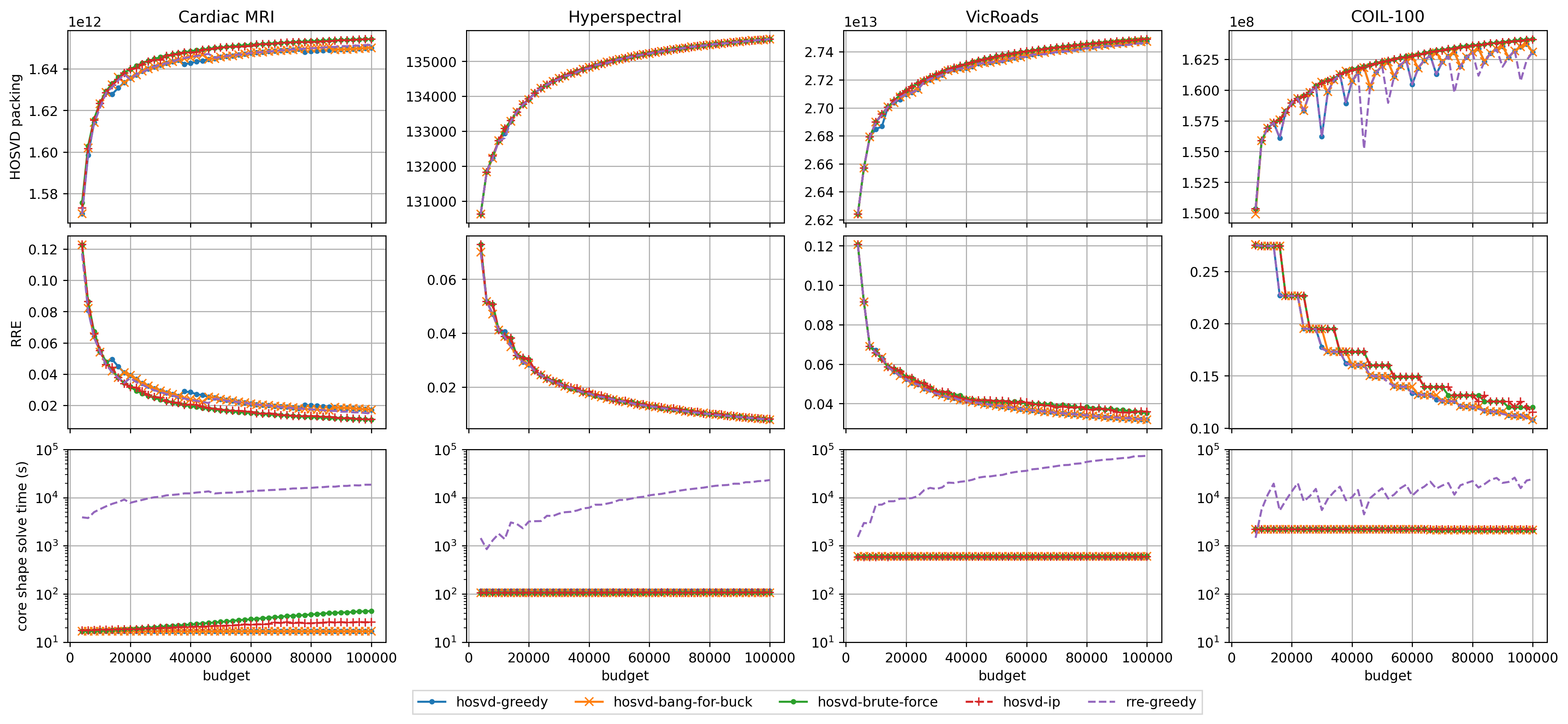
Figure 2: Comparison of five core shape solvers on four real-world tensors (columns) for increasing values of the Tucker decomposition size budget $c\leq 100,000$. The plots in the top row are the HOSVD Tucker packing objective value $f(\mathbf{r})$ for the core shape solutions $\mathbf{r}$, the middle row is the RRE, and the bottom row is the running time of each algorithm in seconds.

We compare several algorithms for computing core shapes for size-constrained Tucker decompositions on four real-world tensors (see Table 1). These experiments demonstrate the effectiveness of using the surrogate loss $\widetilde{L}(\bm{\mathscr{X}},\mathbf{r})$ in place of the true relative reconstruction error (RRE), both in terms of solution quality and running time. All of the experiments use NumPy (Harris et al., 2020) with an Intel Xeon W-1235 processor (3.7 GHz, 8.25MB cache) and 128GB of RAM.

Table 1: Statistics for tensor datasets used in experiments.

tensor	shape	size
cardiac mri	$256\times 256\times 14\times 20$	$18,350,080$
hyperspectral	$1024\times 1344\times 33$	$45,416,488$
vicroads	$1084\times 2033\times 96$	$211,562,112$
coil-100	$7200\times 128\times 128\times 3$	$353,894,400$

6.1 Algorithms

The first four algorithms we consider are based on HOSVD Tucker packing: they compute the mode-$n$ singular values $\sigma_{i_{n}}^{(n)}$ and take $\mathbf{a}^{(n)}=\{(\sigma_{i_{n}}^{(n)})^{2}\}_{i_{n}=1}^{I_{n}}$ as input to their Tucker packing instance. The fifth is a commonly used greedy algorithm that computes true losses $L(\bm{\mathscr{X}},\mathbf{r})$ at each step.

HOSVD-IP is the TuckerPackingSolver algorithm with $\varepsilon=0.25$, but we use the integer programming solver in scipy.optimize.mlip to solve each budget split subproblem instead of the PTAS in Grandoni et al. (2014).

HOSVD-greedy maximizes the same packing objective by repeating $\mathbf{r}\leftarrow\operatorname*{arg\,max}_{\mathbf{r}^{\prime}\in N(\mathbf{r})}f(\mathbf{r}^{\prime})$, where $N(\mathbf{r})$ is the set of neighboring feasible core shapes $\mathbf{r^{\prime}}=\mathbf{r}+\mathbf{e}_{n}$ and $\mathbf{e}_{n}\in\{0,1\}^{N}$ is a standard unit vector. This is Algorithm 3.1 in Ehrlacher et al. (2021) with additional budget constraints.

HOSVD-bang-for-buck is analogous to HOSVD-greedy, but it increments the dimension in each step that maximizes $(f(\mathbf{r}^{\prime})-f(\mathbf{r}))/(\text{cost}(\mathbf{r}^{\prime})-\text{cost}(\mathbf{r}))$, where $\text{cost}(\mathbf{r})$ is the size of the rank-$\mathbf{r}$ Tucker decomposition.

HOSVD-brute-force exhaustively checks all feasible core shapes and outputs the maximum Tucker packing objective.

RRE-greedy constructs the core shape by computing $O(N)$ rank-$\mathbf{r}^{\prime}$ Tucker decompositions in each step and incrementing the dimension that most improves the RRE, Concretely, the update is $\mathbf{r}\leftarrow\operatorname*{arg\,min}_{\mathbf{r}^{\prime}\in N(\mathbf{r})}L(\bm{\mathscr{X}},\mathbf{r^{\prime}})$, similar to the Greedy-TL algorithm of Hashemizadeh et al. (2020).

6.2 Results

We consider the budgets $c\leq 100,000$ for all tensor datasets. For each $c$, we run each algorithm to get core shape $\mathbf{r}$. Then in Figure 2, we plot the packing objective $f(\mathbf{r})$, the RRE, i.e., $L(\bm{\mathscr{X}},\mathbf{r})/\lVert\bm{\mathscr{X}}\rVert_{\textnormal{F}}^{2}$, and the algorithm running time (including the mode-$n$ singular value computations) as a function of $c$. Each $L(\bm{\mathscr{X}},\mathbf{r})$ computation uses 20 iterations of HOOI.

Cardiac MRI shows that maximizing the HOSVD Tucker packing objective $f(\mathbf{r})$ can give noticeably better RRE than RRE-greedy, while also running 1000x faster. If we take a closer look at the core shapes these algorithms output, HOSVD-{brute-force, IP} always return core shapes of the form $(x,y,z,1)$, whereas the greedy algorithms allocate budget to the time dimension as $c$ increases, e.g., $(x,y,z,3)$. Increases in the fourth dimension correspond to points of degradation in $f(\mathbf{r})$ and RRE in Figure 2.

This tensor is also small enough to see differences in the running times of the HOSVD packing algorithms. In particular, we see (1) that there is a fixed cost for computing the $\sigma_{i_{n}}^{(n)}$’s, and (2) that HOSVD-{greedy, bang-for-buck} are faster than HOSVD-IP, which is faster than HOSVD-brute-force. All algorithms are significantly faster than RRE-greedy.

Hyperspectral shows that the surrogate loss $\widetilde{L}(\bm{\mathscr{X}},\mathbf{r})$ and RRE can guide greedy algorithms to the same core shapes, and that HOSVD-greedy can achieve maximum the Tucker packing objective. We see that computing the higher-order singular values becomes the bottleneck for the HOSVD solvers, not solving the packing instances themselves.

VicRoads shows a clear gap between RRE and the surrogate loss. While HOSVD-{greedy, bang-for-buck} are suboptimal in the packing objective, they achieve the same RRE as the 100x slower RRE-greedy algorithm. This data demonstrates a shortcoming of the surrogate loss, but also shows that higher-order singular values can still be effective.

COIL-100 is perhaps the most interesting tensor because it shows the non-monotonic behavior of greedy HOSVD Tucker packing algorithms. Similar to cardiac MRI, every time a greedy core shape solver increases the dimension of the first index (corresponding to the number of objects), the packing objective $f(\mathbf{r})$. This effect also appears in the RRE plots, but it happens in the opposite direction.

Appendix A Missing analysis from Section 3

A.1 Proof of Theorem 3.2

A.1.1 Upper bounding the reconstruction error

For any Tucker decomposition $\bm{\mathscr{X}}=\bm{\mathscr{G}}\times_{1}\mathbf{A}^{(1)}\times_{2}\cdots\times_{N}\mathbf{A}^{(N)}\in\mathbb{R}^{I_{1}\times\dots\times I_{N}}$, the mode-$n$ unfolding of $\bm{\mathscr{X}}$ can be written as

$$\mathbf{X}_{(n)}=\mathbf{A}^{(n)}\mathbf{G}_{(n)}\left(\mathbf{A}^{(1)}\otimes\cdots\mathbf{A}^{(n-1)}\otimes\mathbf{A}^{(n+1)}\otimes\cdots\otimes\mathbf{A}^{(N)}\right)^{\intercal}.$$ (18)

This is the corrected version of Equation (4.2) in Kolda & Bader (2009).

Lemma A.1 (De Lathauwer et al. (2000a, Property 10)).

For any $\bm{\mathscr{X}}\in\mathbb{R}^{I_{1}\times\cdots\times I_{N}}$ and $n\in[N]$, let $\sigma^{(n)}_{1}\geq\sigma^{(n)}_{2}\dots\geq\sigma^{(n)}_{I_{n}}$ denote the singular values of $\mathbf{X}_{(n)}$. Then, for any core shape $\mathbf{r}=(R_{1},R_{2},\dots,R_{N})\in[I_{1}]\times[I_{2}]\times\dots\times[I_{N}]$, we have

$$L(\bm{\mathscr{X}},\mathbf{r}) \leq\lVert\bm{\mathscr{X}}-\widehat{\bm{\mathscr{X}}}_{\textnormal{HOSVD}(\mathbf{r})}\rVert_{\textnormal{F}}^{2}$$

$$\leq\sum_{i_{1}=R_{1}+1}^{I_{1}}\left(\sigma_{i_{1}}^{(1)}\right)^{2}+\sum_{i_{2}=R_{2}+1}^{I_{2}}\left(\sigma_{i_{2}}^{(2)}\right)^{2}+\cdots+\sum_{i_{N}=R_{N}+1}^{I_{N}}\left(\sigma_{i_{N}}^{(N)}\right)^{2}.$$

Proof.

Let the HOSVD of $\bm{\mathscr{X}}=\bm{\mathscr{S}}\times_{1}\mathbf{U}^{(1)}\times_{2}\cdots\times_{N}\mathbf{U}^{(N)}$ as in Theorem 3.1. Let $\overline{\bm{\mathscr{S}}}$ denote the truncated version of $\bm{\mathscr{S}}$ with respect to core shape $\mathbf{r}$ such that

$$\overline{s}_{i_{1}\dots i_{N}}=\begin{cases}s_{i_{1}\dots i_{N}}&$\text{if $i_{n}\leq R_{n}$ for all $n\in[N]$},$\\ 0&\text{otherwise}.\end{cases}$$

Let $\overline{\bm{\mathscr{X}}}=\overline{\bm{\mathscr{S}}}\times_{1}\mathbf{U}^{(1)}\times_{2}\dots\times_{N}\mathbf{U}^{(N)}$. Summing over all dimensions $n\in[N]$ and using the HOSVD results in Theorem 3.1,

$$\lVert\bm{\mathscr{S}}-\overline{\bm{\mathscr{S}}}\rVert_{\textnormal{F}}^{2} \leq\sum_{n=1}^{N}\sum_{j=R_{n}+1}^{I_{n}}\lVert\left(\bm{\mathscr{S}}-\overline{\bm{\mathscr{S}}}\right)_{i_{n}=j}\rVert_{\textnormal{F}}^{2}$$

$$=\sum_{n=1}^{N}\sum_{j=R_{n}+1}^{I_{n}}\lVert\bm{\mathscr{S}}_{i_{n}=j}\rVert_{\textnormal{F}}^{2}$$

$$=\sum_{n=1}^{N}\sum_{i_{n}=R_{n}+1}^{I_{n}}\left(\sigma_{i_{n}}^{(n)}\right)^{2}.$$

We have $\lVert\bm{\mathscr{S}}-\overline{\bm{\mathscr{S}}}\rVert_{\textnormal{F}}^{2}=\lVert\mathbf{S}_{(n)}-\overline{\mathbf{S}}_{(n)}\rVert_{\textnormal{F}}^{2}$ for all values of $n$. Further, since the Kronecker product of two orthogonal matrices is also orthogonal and multiplication by an orthogonal matrix does not affect the Frobenius norm, Equation Equation 18 implies that

$$\lVert\mathbf{S}_{(n)}-\overline{\mathbf{S}}_{(n)}\rVert_{\textnormal{F}}^{2} =\lVert\mathbf{U}_{(n)}(\mathbf{S}_{(n)}-\overline{\mathbf{S}}_{(n)})(\mathbf{U}_{(1)}\otimes\dots\otimes\mathbf{U}_{(n-1)}\otimes\mathbf{U}_{(n+1)}\otimes\cdots\otimes\mathbf{U}_{(N)})^{\intercal}\rVert_{\textnormal{F}}^{2}$$

$$=\lVert\bm{\mathscr{X}}-\overline{\bm{\mathscr{X}}}\rVert_{\textnormal{F}}^{2}.$$

Observing that $\overline{\bm{\mathscr{X}}}=\widehat{\bm{\mathscr{X}}}_{\textnormal{HOSVD}(\mathbf{r})}$ by the definition of TuckerHOSVD in Algorithm 1 and putting everything together,

$$L(\bm{\mathscr{X}},\mathbf{r})\leq\lVert\bm{\mathscr{X}}-\widehat{\bm{\mathscr{X}}}_{\textnormal{HOSVD}(\mathbf{r})}\rVert_{\textnormal{F}}^{2}=\lVert\bm{\mathscr{X}}-\overline{\bm{\mathscr{X}}}\rVert_{\textnormal{F}}^{2}=\lVert\bm{\mathscr{S}}-\overline{\bm{\mathscr{S}}}\rVert_{\textnormal{F}}^{2}\leq\sum_{n=1}^{N}\sum_{i_{n}=R_{n}+1}^{I_{n}}\left(\sigma_{i_{n}}^{(n)}\right)^{2},$$

which completes the proof. ∎

A.1.2 Lower bounding the reconstruction error

Theorem A.2 (Eckart & Young (1936)).

Let $\mathbf{A}\in\mathbb{R}^{n\times d}$ with $n\geq d$ and singular values $\sigma_{1}\geq\sigma_{2}\geq\dots\geq\sigma_{d}\geq 0$. Let $\mathbf{A}_{k}$ be the best rank-$k$ approximation of $\mathbf{A}$ in the Frobenius norm. Then

$$\left\lVert\mathbf{A}-\mathbf{A}_{k}\right\rVert_{\textnormal{F}}^{2}=\sum_{i=k+1}^{d}\sigma_{i}^{2}.$$

Lemma A.3.

For any $\bm{\mathscr{X}}\in\mathbb{R}^{I_{1}\times\cdots\times I_{N}}$ and $n\in[N]$, let $\sigma^{(n)}_{1}\geq\dots\geq\sigma^{(n)}_{I_{n}}$ denote the singular values of $\mathbf{X}_{(n)}$. For every core shape $\mathbf{r}=(R_{1},R_{2},\dots,R_{N})\in[I_{1}]\times[I_{2}]\times\dots\times[I_{N}]$, we have

$$L(\bm{\mathscr{X}},\mathbf{r})\geq\max_{n\in[N]}\sum_{i_{n}=R_{n}+1}^{I_{n}}\left(\sigma_{i_{n}}^{(n)}\right)^{2}.$$

Proof.

Let the core tensor and factors that minimize $L(\bm{\mathscr{X}},\mathbf{r})$ be $\bm{\mathscr{G}}\in\mathbb{R}^{R_{1}\times\dots\times R_{N}}$ and $\mathbf{A}^{(n)}\in\mathbb{R}^{I_{n}\times R_{n}}$, i.e.,

$$L(\bm{\mathscr{X}},\mathbf{r})=\lVert\bm{\mathscr{X}}-\bm{\mathscr{G}}\times_{1}\mathbf{A}^{(1)}\times_{2}\dots\times_{N}\mathbf{A}^{(N)}\rVert_{\textnormal{F}}^{2}.$$

Let $\widehat{\bm{\mathscr{X}}}=\bm{\mathscr{G}}\times_{1}\mathbf{A}^{(1)}\times_{2}\dots\times_{N}\mathbf{A}^{(N)}$. Equation Equation 18 and the dimensions of $\mathbf{A}^{(n)}\in\mathbb{R}^{I_{n}\times R_{n}}$ imply that

$$\textnormal{rank}\left(\widehat{\mathbf{X}}_{(n)}\right)\leq\textnormal{rank}\left(\mathbf{A}^{(n)}\right)\leq R_{n},$$

since $R_{n}\leq I_{n}$. The Eckart–Young–Mirsky theorem (Theorem A.2) with the characterization of $\sigma_{i}^{(n)}$ in Theorem 3.1 gives

$$\lVert\bm{\mathscr{X}}-\widehat{\bm{\mathscr{X}}}\rVert_{\textnormal{F}}^{2}=\lVert\mathbf{X}_{(n)}-\widehat{\mathbf{X}}_{(n)}\rVert_{\textnormal{F}}^{2}\geq\sum_{i_{n}=R_{n}+1}^{I_{n}}\left(\sigma_{i_{n}}^{(n)}\right)^{2}.$$ (19)

Equation Equation 19 holds for all values of $n$, so take the equation that maximizes the right-hand side. ∎

A.1.3 Combining the results

Now we combine Lemma A.1 and Lemma A.3 to give an approximation inequality that is true for all core shapes.

Lemma A.4.

For any $\bm{\mathscr{X}}\in\mathbb{R}^{I_{1}\times\cdots\times I_{N}}$ and any core shape $\mathbf{r}=(R_{1},R_{2},\dots,R_{N})\in[I_{1}]\times[I_{2}]\times\dots\times[I_{N}]$, we have

$$\frac{1}{N}\cdot\widetilde{L}(\bm{\mathscr{X}},\mathbf{r})\leq L(\bm{\mathscr{X}},\mathbf{r})\leq\widetilde{L}(\bm{\mathscr{X}},\mathbf{r}),$$

where $\widetilde{L}(\bm{\mathscr{X}},\mathbf{r})$ is defined in Equation Equation 2.

Proof.

Summing Equation Equation 19 in the proof of Lemma A.3 over all values of $n\in[N]$ gives

$$\sum_{n=1}^{N}\sum_{i_{n}=R_{n}+1}^{I_{n}}\left(\sigma_{i_{n}}^{(n)}\right)^{2}\leq N\cdot L(\bm{\mathscr{X}},\mathbf{r})\implies\frac{1}{N}\cdot\widetilde{L}(\bm{\mathscr{X}},\mathbf{r})\leq L(\bm{\mathscr{X}},\mathbf{r}).$$ (20)

The upper bound $L(\bm{\mathscr{X}},\mathbf{r})\leq\widetilde{L}(\bm{\mathscr{X}},\mathbf{r})$ is a restatement of Lemma A.1. ∎

See 3.2

Proof.

The proof follows by combining Lemma A.1 and Equation Equation 20. ∎

A.2 Proof of Lemma 3.4

See 3.4

Proof.

For any $n$, we have

$$\sum_{i_{n}=1}^{I_{n}}\left(\sigma_{i_{n}}^{(n)}\right)^{2}=\lVert\mathbf{X}_{(n)}\rVert_{\textnormal{F}}^{2}=\lVert\bm{\mathscr{X}}\rVert_{\textnormal{F}}^{2}.$$

Therefore, for any choice of $\mathbf{r}=(R_{1},R_{2},\dots,R_{N})$, we have

$$\left[\sum_{n=1}^{N}\sum_{i_{n}=1}^{R_{n}}\left(\sigma_{i_{n}}^{(n)}\right)^{2}\right]+\left[\sum_{n=1}^{N}\sum_{i_{n}=R_{n}+1}^{I_{n}}\left(\sigma_{i_{n}}^{(n)}\right)^{2}\right]=N\left\lVert\bm{\mathscr{X}}\right\rVert_{\textnormal{F}}^{2}.$$

This is a constant value that only depends on $\bm{\mathscr{X}}$, so minimizing $\widetilde{L}(\bm{\mathscr{X}},\mathbf{r})$ is equivalent to maximizing the packing version since both problems optimize over the same set $F$.

Lastly, we have

$$\widetilde{L}\left(\bm{\mathscr{X}},\widetilde{\mathbf{r}}^{*}\right)\leq\widetilde{L}\left(\bm{\mathscr{X}},\mathbf{r}^{*}\right)\leq N\cdot L\left(\bm{\mathscr{X}},\mathbf{r}^{*}\right),$$

where the first inequality follows from optimizing the surrogate loss and the second inequality follows from Lemma A.4 since that result holds for all core shapes. ∎

A.3 Hardness

Definition A.5.

Let $N\geq 2$ be an even integer and $w_{1},\dots,w_{N}\geq 1$ be integers. The EQUIPARTITION problem asks to determine whether there exists a subset $S\subseteq[N]$ of size $n/2$ such that

$$\sum_{i\in S}w_{i}=\sum_{i\in[N]\setminus S}w_{i}.$$

Lemma A.6 (Garey & Johnson 1979, SP12).

EQUIPARTITION is NP-complete.

We now give a reduction from the equipartition problem to the Tucker packing problem.

See 3.6

Proof.

Let $T,w_{1},\dots,w_{T}$ be an instance of EQUIPARTITION where $w_{n}\geq 2$ for all $n\in[T]$. Notice that the assumption $w_{n}\geq 2$ is without loss of generality because we can multiply all of the values $w_{1},\dots,w_{T}$ by two.

Let $M=\sum_{n\in[T]}w_{n}$ be the sum of all weights, and let $N\geq T$ be the smallest integer such that $2^{N-T/2}>4(N-T)+3M/2$. Now we construct an instance of the Tucker packing problem. For each $n\in[T]$, let:

• $I_{n}=w_{n}$

• $a^{(n)}_{1}=2M$

• $a^{(n)}_{2}=M+w_{n}$

• $a^{(n)}_{i_{n}}=0$, for all $i_{n}\in[I_{n}]\setminus\{1,2\}$

Next, for each $n\in[N]\setminus[T]$, let:

• $I_{n}=2$

• $a^{(n)}_{1}=a^{(n)}_{2}=2M$

Finally, set the budget to be $c=2^{N-T/2}+4(N-T)+3M/2$.

First, notice that this is a valid instance of the Tucker packing problem since $a^{(n)}_{1}\geq a^{(n)}_{2}\geq\cdots\geq a^{(n)}_{I_{n}}$ for all $n\in[N]$. Further, since $N=O(T\cdot\log_{2}(3M/2))$ and $a^{(n)}_{i_{n}}=0$ for $i_{n}\in[I_{n}]\setminus\{1,2\}$, the size of the description of this problem is polynomial in the size of the description of the corresponding EQUIPARTITION problem.

Now we consider a decision version of this Tucker packing problem in which we are asked to determine whether there exists a feasible solution $(R_{1},\ldots,R_{N})$ such that

$$\sum_{n=1}^{N}\sum_{i_{n}=1}^{R_{n}}a_{i_{n}}^{(n)}\geq M(4N-3T/2)+M/2.$$ (21)

We show that a positive answer to the decision version of the Tucker packing problem in  Equation 21 implies a positive answer to the EQUIPARTITION problem and vice versa.

Suppose the answer to the decision version of the Tucker packing problem is YES, and $\mathbf{r}^{*}$ is an optimal solution such that

$$\sum_{n=1}^{N}\sum_{i_{n}=1}^{R^{*}_{n}}a_{i_{n}}^{(n)}\geq M(4N-3T/2)+M/2\quad~{}~{}\text{and}~{}~{}\quad\prod_{n=1}^{N}R^{*}_{n}+\sum_{n=1}^{N}I_{n}R^{*}_{n}\leq c.$$

Since

$$c=2^{N-T/2}+4(N-T)+3M/2<2\cdot 2^{N-T/2}=2^{N-T/2+1},$$

there are at most $N-T/2$ values of $R^{*}_{n}$ such that $R^{*}_{n}\geq 2$. Further, since $a^{(n)}_{i_{n}}=0$ for all $i_{n}\geq 3$, we never have $R^{*}_{n}>2$ in a minimal optimal solution. It follows that $R^{*}_{n}\in\{1,2\}$ for all $n\in[N]$, and

$$\prod_{n=1}^{N}R^{*}_{n}\leq 2^{N-T/2}.$$

Next, we establish the structure of an optimal solution to this Tucker packing instance. Observe that $\widehat{\mathbf{r}}=(\widehat{R}_{1},\dots,\widehat{R}_{N})$ with $\widehat{R}_{1}=\dots=\widehat{R}_{T}=1$ and $\widehat{R}_{T+1}=\dots=\widehat{R}_{N}=2$ is a feasible solution $\mathbf{r}$ that achieves an objective value of $M(4N-2T)$. Now consider any feasible solution in which there exists $i\in[T]$ and $j\in[N]\setminus[T]$ such that $R_{i}=2$ and $R_{j}=1$. If we switch the values of $R_{i}$ and $R_{j}$, then the cost decreases by $w_{i}-2\geq 0$ (i.e., the solution is still feasible), and the objective value increases by $M-w_{i}>0$. Therefore, since $\widehat{\mathbf{r}}$ is feasible, in an optimal solution we have $R_{n}=2$ for all $n\in[N]\setminus[T]$ and at most $T/2$ of the $R_{n}$’s for $n\in[T]$ are equal to two.

Let $S=\{i\in[T]:R^{*}_{i}=2\}$. Then by construction we have

$$\sum_{n\in S}a^{(n)}_{2}=\sum_{n\in S}(M+w_{n})=M\lvert S\rvert+\sum_{n\in S}w_{n}<M(\lvert S\rvert+1).$$

Moreover, since the answer to the decision problem is YES and in an optimal solution we have $R_{n}^{*}=2$ for all $n\in[N]\setminus[T]$, it follows that

$$\sum_{n\in S}a^{(n)}_{2} =f(\mathbf{r}^{*})-\sum_{n=1}^{N}a_{1}^{(n)}-\sum_{n=T+1}^{N}a_{2}^{(n)}$$ (22)

$$=f(\mathbf{r}^{*})-2NM-2(N-T)M$$

$$\geq M(4N-3T/2)+M/2-2NM-2(N-T)M$$

$$=MT/2+M/2.$$

Therefore,

$$M(\lvert S\rvert+1)>MT/2+M/2,$$

which implies $\lvert S\rvert>T/2-1/2$, so $\lvert S\rvert\geq T/2$ since $\lvert S\rvert$ and $T/2$ are integers. Using the characterization above about an optimal solution together with the fact that the budget is strictly less than $2^{N-T/2+1}$ gives us $\lvert S\rvert\leq T/2$. Thus, a YES to the decision problem implies that $\lvert S\rvert=T/2$, which further implies $\prod_{n=1}^{N}R^{*}_{n}=2^{N-T/2}$.

It then follows from our choice of budget $c$ that

$$\sum_{n=1}^{N}I_{n}R^{*}_{n}\leq c-2^{N-T/2}=4(N-T)+3M/2,$$

which then by the definition of $I_{n}$ implies that

$$\left(\sum_{n=1}^{T}w_{n}R_{n}^{*}+\sum_{n=T+1}^{N}2R_{n}^{*}\right)=\left(M+\sum_{n\in S}w_{n}\right)+4(N-T)\leq 4(N-T)+3M/2\implies\sum_{n\in S}w_{n}\leq M/2.$$

Furthermore, using (22), the definition of the $a_{i_{n}}^{(n)}$’s, and the fact that $\lvert S\rvert=T/2$, we have

$$\sum_{n\in S}a_{2}^{(n)}=\sum_{n\in S}(M+w_{n})=|S|M+\sum_{n\in S}w_{n}\geq MT/2+M/2\implies\sum_{n\in S}w_{n}\geq M/2.$$

Putting everything together, we get $\sum_{n\in S}w_{n}=M/2$. Thus, $S$ is a solution for the EQUIPARTITION problem.

Now suppose the answer to the EQUIPARTITION problem is YES. Let $S\subseteq[T]$ such that $|S|=T/2$ and $\sum_{n\in S}w_{n}=M/2$. Construct $\mathbf{r}^{*}$ as follows: For each $n\in S\cup([N]\setminus[T])$, set $R^{*}_{n}=2$; for each $n\in[T]\setminus S$, set $R^{*}_{n}=1$.

Then, by the definitions of $I_{n}$ and $a_{i_{n}}^{(n)}$ above, we have

$$\sum_{n=1}^{N}\sum_{i_{n}=1}^{R^{*}_{n}}a_{i_{n}}^{(n)}\geq M(4N-3T/2)+M/2\quad~{}~{}\text{and}~{}~{}\quad\prod_{n=1}^{N}R^{*}_{n}+\sum_{n=1}^{N}I_{n}R^{*}_{n}\leq c,$$

which completes the proof. ∎

A.4 Translating between approximate maximization and minimization

We prove an additive-error guarantee that shows how a $(1-\varepsilon^{\prime})$-approximate solution to the Tucker packing problem, i.e., a core shape $\mathbf{r}\in[I_{1}]\times\dots\times[I_{N}]$, can lead to an increase in the surrogate loss objective.

See 3.7

Proof.

Let $\varepsilon^{\prime}=\varepsilon/N$ and $\widetilde{\mathbf{r}}^{*}$ be the optimal shape for the surrogate loss $\widetilde{L}$. If $\mathbf{r}=(R_{1},\dots,R_{N})$ is a $(1-\varepsilon^{\prime})$-approximation to the Tucker packing problem, it follows that

$$\frac{\widetilde{L}(\bm{\mathscr{X}},\mathbf{r})}{\left\lVert\bm{\mathscr{X}}\right\rVert_{\textnormal{F}}^{2}} =\frac{N\left\lVert\bm{\mathscr{X}}\right\rVert_{\textnormal{F}}^{2}-\sum_{n=1}^{N}\sum_{i_{n}=1}^{R_{n}}\left(\sigma_{i_{n}}^{(n)}\right)^{2}}{\left\lVert\bm{\mathscr{X}}\right\rVert_{\textnormal{F}}^{2}}$$

$$\leq\frac{N\left\lVert\bm{\mathscr{X}}\right\rVert_{\textnormal{F}}^{2}-\left(1-\varepsilon^{\prime}\right)\sum_{n=1}^{N}\sum_{i_{n}=1}^{\widetilde{R}^{*}_{n}}\left(\sigma_{i_{n}}^{(n)}\right)^{2}}{\left\lVert\bm{\mathscr{X}}\right\rVert_{\textnormal{F}}^{2}}$$

$$=\frac{\widetilde{L}\left(\bm{\mathscr{X}},\widetilde{\mathbf{r}}^{*}\right)}{\left\lVert\bm{\mathscr{X}}\right\rVert_{\textnormal{F}}^{2}}+\varepsilon^{\prime}\left(N-\frac{\widetilde{L}\left(\bm{\mathscr{X}},\widetilde{\mathbf{r}}^{*}\right)}{\left\lVert\bm{\mathscr{X}}\right\rVert_{\textnormal{F}}^{2}}\right)$$

$$\leq\frac{\widetilde{L}\left(\bm{\mathscr{X}},\widetilde{\mathbf{r}}^{*}\right)}{\left\lVert\bm{\mathscr{X}}\right\rVert_{\textnormal{F}}^{2}}+\varepsilon.$$

Theorem 3.2 gives us $L(\bm{\mathscr{X}},\mathbf{r})\leq\widetilde{L}(\bm{\mathscr{X}},\mathbf{r})\leq N\cdot L(\bm{\mathscr{X}},\mathbf{r})$. By definition $\widetilde{L}\left(\bm{\mathscr{X}},\widetilde{\mathbf{r}}^{*}\right)\leq\widetilde{L}\left(\bm{\mathscr{X}},\mathbf{r}^{*}\right)$, so we have

$$\textnormal{RRE}(\bm{\mathscr{X}},\mathbf{r})=\frac{L(\bm{\mathscr{X}},\mathbf{r})}{\left\lVert\bm{\mathscr{X}}\right\rVert_{\textnormal{F}}^{2}}\leq\frac{\widetilde{L}(\bm{\mathscr{X}},\mathbf{r})}{\left\lVert\bm{\mathscr{X}}\right\rVert_{\textnormal{F}}^{2}}\leq\frac{\widetilde{L}\left(\bm{\mathscr{X}},\widetilde{\mathbf{r}}^{*}\right)}{\left\lVert\bm{\mathscr{X}}\right\rVert_{\textnormal{F}}^{2}}+\varepsilon\leq\frac{\widetilde{L}\left(\bm{\mathscr{X}},\mathbf{r}^{*}\right)}{\left\lVert\bm{\mathscr{X}}\right\rVert_{\textnormal{F}}^{2}}+\varepsilon\leq N\cdot\frac{L\left(\bm{\mathscr{X}},\mathbf{r}^{*}\right)}{\left\lVert\bm{\mathscr{X}}\right\rVert_{\textnormal{F}}^{2}}+\varepsilon=N\cdot\textnormal{RRE}(\bm{\mathscr{X}},\mathbf{r}^{*})+\varepsilon,$$

as desired. ∎

Appendix B Missing analysis from Section 4

B.1 Proof of Lemma 4.3

See 4.3

Proof.

Let $k_{n}\geq 0$ be the largest integer such that $(1+\varepsilon)^{k_{n}}\leq R^{*}_{n}$ for each $n\in[N]$. Further, let

$$\widehat{R}_{n}=\left\lceil(1+\varepsilon)^{k_{n}}\right\rceil.$$

Since $R^{*}_{n}$ is an integer, we know that $\widehat{R}_{n}\leq R^{*}_{n}$. Therefore, because $F$ is downwards closed, $\widehat{\mathbf{r}}=(\widehat{R}_{1},\dots,\widehat{R}_{N})$ is a feasible solution to (10). It follows that

$$f(\widehat{\mathbf{r}})\leq f(\mathbf{r}^{(\varepsilon)}).$$ (23)

Now we will show that $f(\mathbf{r}^{*})\leq(1+\varepsilon)f(\widehat{\mathbf{r}})$. Since $a_{1}^{(n)}\geq\dots\geq a_{I_{n}}^{(n)}\geq 0$ for all $n\in[N]$, we have

$$(1+\varepsilon)\sum_{i_{n}=1}^{\widehat{R}_{n}}a_{i_{n}}^{(n)}\geq\sum_{i_{n}=1}^{\lfloor(1+\varepsilon)\widehat{R}_{n}\rfloor}a_{i_{n}}^{(n)}.$$ (24)

By the definition of $k_{n}$, it follows that

$$(1+\varepsilon)\widehat{R}_{n} =(1+\varepsilon)\left\lceil(1+\varepsilon)^{k_{n}}\right\rceil$$

$$\geq(1+\varepsilon)^{k_{n}+1}$$

$$>R_{n}^{*}.$$

Since $R_{n}^{*}$ is an integer, we have $\lfloor(1+\varepsilon)\widehat{R}_{n}\rfloor\geq R_{n}^{*}$. Therefore, using Equation Equation 25 we have

$$(1+\varepsilon)\sum_{i_{n}=1}^{\widehat{R}_{n}}a_{i_{n}}^{(n)}\geq\sum_{i_{n}=1}^{R_{n}^{*}}a_{i_{n}}^{(n)}.$$ (25)

Finally, summing over $n\in[N]$ and using Equation Equation 23 gives us

$$(1+\varepsilon)f(\mathbf{\widehat{r}})\geq f(\mathbf{r}^{*})\implies f(\mathbf{r}^{(\varepsilon)})\geq(1+\varepsilon)^{-1}f(\mathbf{r}^{*}).$$

Algorithm.

Now we design and analyze a simple algorithm to solve the grid-search problem in Equation 10. First observe that

$$|S_{n}^{(\varepsilon)}|=1+\left\lfloor\log_{1+\varepsilon}(I_{n})\right\rfloor=1+\left\lfloor\frac{\log_{2}(I_{n})}{\log_{2}(1+\varepsilon)}\right\rfloor.$$

It follows that the number of feasible solutions for Problem (10) is

$$O\left(\prod_{n=1}^{N}\left(1+\frac{\log_{2}(I_{n})}{\log_{2}(1+\varepsilon)}\right)\right)=O\left(\frac{1}{\log_{2}^{N}(1+\varepsilon)}\prod_{n=1}^{N}\left(1+\log_{2}(I_{n})\right)\right),$$

since $\log_{2}(1+\varepsilon)\leq 1$ for $\varepsilon\leq 1$. Further, observing that $\log_{2}(1+\varepsilon)\geq\varepsilon$ for $0<\varepsilon\leq 1$ implies a bound of

$$O\left(\frac{1}{\varepsilon^{N}}\prod_{n=1}^{n}\left(1+\log_{2}(I_{n})\right)\right)$$

on the number of feasible solutions.

After computing the prefix sums for elements of $S_{n}^{(\varepsilon)}$’s, we can iterate over the elements of $S_{1}^{(\varepsilon)}\times\cdots\times S_{N}^{(\varepsilon)}$ in the lexicographical order, check for feasibility, and compute the objective value $f(\mathbf{r})$ for any candidate solution in amortized time $O(1)$. Finally, note that the prefix sums for elements of $S_{n}^{(\varepsilon)}$ can be computed in $O(I_{n})$ time. ∎

Rationale for two different types of budget splits in Algorithm 2.

Instead of considering two different budget splitting methods (i.e., with $c_{\text{factor}}$ and $c_{\text{core}}$), one could just consider the budget splits $c_{\text{factor}}\in[\sum_{n=1}^{N}I_{n}^{2}]$ over problems of the form:

maximize $$f(\mathbf{r})$$

subject to $$\textstyle\prod_{n=1}^{N}R_{n}\leq c-c_{\text{factor}}$$

$$\textstyle\sum_{n=1}^{N}I_{n}R_{n}\leq c_{\text{factor}}$$

$$R_{n}\in[I_{n}]\hskip 28.45274pt\forall n\in[N]$$

This approach also gives a PTAS. The running time, however, is $O((\sum_{n=1}^{N}I_{n}^{2})(\sum_{n=1}^{N}I_{n})^{O\left(1/\varepsilon\right)})$. In contrast, the running time of Algorithm 2 is $O((\log_{1+\varepsilon}(c)+\left\lceil 1/\varepsilon\right\rceil\sum_{n=1}^{N}I_{n})(\sum_{n=1}^{N}I_{n})^{O\left(1/\varepsilon\right)})$. Note that $c\leq\sum_{n=1}^{N}I_{n}^{2}+\prod_{n=1}^{N}I_{n}$. Therefore, $\log_{1+\varepsilon}(c)=O(\frac{1}{\varepsilon}\sum_{n=1}^{N}\log_{2}(I_{n}))\ll\left\lceil 1/\varepsilon\right\rceil\sum_{n=1}^{N}I_{n}$, where the first equality follows from the concavity of the logarithm function. Thus, our running time is $O((\left\lceil 1/\varepsilon\right\rceil\sum_{n=1}^{N}I_{n})(\sum_{n=1}^{N}I_{n})^{O\left(1/\varepsilon\right)})$, which is always smaller than $O((\sum_{n=1}^{N}I_{n}^{2})(\sum_{n=1}^{N}I_{n})^{O\left(1/\varepsilon\right)})$.

Appendix C Tree tensor networks

Remark C.1.

Although the tree tensor network is considered for general Hilbert spaces and has been defined in full generality using the tensor network notations (see, e.g., Hackbusch (2019, Chapter 11) and Krämer (2020, Chapter 3)), we consider finite-dimensional Euclidean spaces to keep our notation simple.

Remark C.2.

Theorem 5.6 is implied by Lemma 4.3.

Figure 3: Tree tensor network corresponding to a Tucker decomposition.

Example (Tucker decomposition).

Tucker decomposition corresponds to a tree tensor of depth one. For example, the tree tensor in Figure 3 consists of matrices $\mathbf{A}_{1}\in\mathbb{R}^{I_{1}\times R_{e_{1}}},\mathbf{A}_{2}\in\mathbb{R}^{I_{2}\times R_{e_{2}}},\mathbf{A}_{3}\in\mathbb{R}^{I_{3}\times R_{e_{3}}},\mathbf{A}_{4}\in\mathbb{R}^{I_{4}\times R_{e_{4}}}$, and tensor $\bm{\mathscr{T}}_{v}\in\mathbb{R}^{R_{e_{1}}\times R_{e_{2}}\times R_{e_{3}}\times R_{e_{4}}}$. The corresponding reconstruction is

$$\widehat{\bm{\mathscr{X}}}=\bm{\mathscr{T}}_{v}\times_{e_{4}}\mathbf{A}_{4}\times_{e_{3}}\mathbf{A}_{3}\times_{e_{2}}\mathbf{A}_{2}\times_{e_{1}}\mathbf{A}_{1}.$$

Figure 4: Tree tensor network example corresponding to a hierarchical Tucker decomposition.

Example (Hierarchical Tucker decomposition).

To to better understand Definition 5.1, we give an example for a tensor of order $4$. Consider the tree illustrated in Figure 4. This tree tensor network corresponds to matrices $\mathbf{A}_{1}\in\mathbb{R}^{I_{1}\times R_{e_{1}}},\mathbf{A}_{2}\in\mathbb{R}^{I_{2}\times R_{e_{2}}},\mathbf{A}_{3}\in\mathbb{R}^{I_{3}\times R_{e_{3}}},\mathbf{A}_{4}\in\mathbb{R}^{I_{4}\times R_{e_{4}}}$, and tensors $\bm{\mathscr{T}}_{u}\in\mathbb{R}^{R_{e_{1}}\times R_{e_{2}}\times R_{e_{5}}},\bm{\mathscr{T}}_{v}\in\mathbb{R}^{R_{e_{3}}\times R_{e_{4}}\times R_{e_{6}}},\bm{\mathscr{T}}_{w}\in\mathbb{R}^{R_{e_{5}}\times R_{e_{6}}}$. The corresponding reconstruction is

$$\widehat{\bm{\mathscr{X}}}=\bm{\mathscr{T}}_{w}\times_{e_{6}}\bm{\mathscr{T}}_{v}\times_{e_{5}}\bm{\mathscr{T}}_{u}\times_{e_{4}}\mathbf{A}_{4}\times_{e_{3}}\mathbf{A}_{3}\times_{e_{2}}\mathbf{A}_{2}\times_{e_{1}}\mathbf{A}_{1}.$$

Appendix D Experiments

We provide short descriptions about each of the tensor datasets used in the core shape experiments in Section 6, which gives some insight into why the algorithms build the core shapes they do.

Cardiac MRI.

$256\times 256\times 14\times 20$ tensor whose elements are MRI measurements indexed by $(x,y,z,t)$, where $(x,y,z)$ is a point in space and $t$ corresponds to time.

Hyperspectral.

$1024\times 1344\times 33$ tensor of time-lapse hyperspectral radiance images of a nature scene that is undergoing illumination changes (Nascimento et al., 2016).

VicRoads.

$1084\times 2033\times 96$ tensor containing 2033 days of traffic volume data from Melbourne and its surrounding suburbs. This data comes from a network of 1084 road sensors measured in 15 minute intervals (Schimbinschi et al., 2015).

COIL-100.

$7200\times 128\times 128\times 3$ tensor containing 7200 colored photos of 100 different objects (72 images per object) taken at 5-degree rotations (Nene et al., 1996). This is a widely-used dataset in the computer vision research community.

References

- Arthur & Vassilvitskii (2006) Arthur, D. and Vassilvitskii, S. -means++: The advantages of careful seeding. Technical report, Stanford, 2006.
- Bader & Kolda (2022) Bader, B. W. and Kolda, T. G. Tensor toolbox for MATLAB, version 3.4. https://www.tensortoolbox.org/, 2022.
- Battaglino et al. (2018) Battaglino, C., Ballard, G., and Kolda, T. G. A practical randomized CP tensor decomposition. SIAM Journal on Matrix Analysis and Applications, 39(2):876–901, 2018.
- Che & Wei (2019) Che, M. and Wei, Y. Randomized algorithms for the approximations of tucker and the tensor train decompositions. Advances in Computational Mathematics, 45(1):395–428, 2019.
- Cheng et al. (2016) Cheng, D., Peng, R., Liu, Y., and Perros, I. Spals: Fast alternating least squares via implicit leverage scores sampling. Advances in Neural Information Processing Systems, 29, 2016.
- De Lathauwer et al. (2000a) De Lathauwer, L., De Moor, B., and Vandewalle, J. A multilinear singular value decomposition. SIAM Journal on Matrix Analysis and Applications, 21(4):1253–1278, 2000a.