DIFF2: Differential Private Optimization via Gradient Differences
for Nonconvex Distributed Learning

Abstract

Differential private optimization for nonconvex smooth objective is considered. In the previous work, the best known utility bound is $\widetilde{O}(\sqrt{d}/(n\varepsilon_{\mathrm{DP}}))$ in terms of the squared full gradient norm, which is achieved by Differential Private Gradient Descent (DP-GD) as an instance, where $n$ is the sample size, $d$ is the problem dimensionality and $\varepsilon_{\mathrm{DP}}$ is the differential privacy parameter. To improve the best known utility bound, we propose a new differential private optimization framework called DIFF2 (DIFFerential private optimization via gradient DIFFerences) that constructs a differential private global gradient estimator with possibly quite small variance based on communicated gradient differences rather than gradients themselves. It is shown that DIFF2 with a gradient descent subroutine achieves the utility of $\widetilde{O}(d^{2/3}/(n\varepsilon_{\mathrm{DP}})^{4/3})$, which can be significantly better than the previous one in terms of the dependence on the sample size $n$. To the best of our knowledge, this is the first fundamental result to improve the standard utility $\widetilde{O}(\sqrt{d}/(n\varepsilon_{\mathrm{DP}}))$ for nonconvex objectives. Additionally, a more computational and communication efficient subroutine is combined with DIFF2 and its theoretical analysis is also given. Numerical experiments are conducted to validate the superiority of DIFF2 framework.

1 Introduction

Privacy protection has become one of the important components in modern artificial intelligence technologies. Datasets consisted of browsing history, check-in data, medical records, financial records and so on, often contain private information, and then publishing the statistics like trained models or computed gradients on the private datasets causes a leak of the private information. In the recently proposed federated learning framework (Konečnỳ et al., 2016; McMahan et al., 2017), where each client possesses a private local dataset and iteratively exchanges the own models or gradients with the central server, it is crucial to prevent the malicious clients from stealing the private information contained in the local datasets.

Actually, many attacks to steal the private information from the trained models or gradients are known. Major attacks include membership inference attack (Shokri et al., 2017; Yeom et al., 2018; Nasr et al., 2019) and reconstruction attack (Fredrikson et al., 2015; Zhu et al., 2019; Yang et al., 2019; Wang et al., 2019d; Geiping et al., 2020; Zhang et al., 2020b). Membership inference attack aims to infer the presence of the known individual or record in the dataset from the shared statistics of the dataset. Reconstruction attack aims to reconstruct the data samples of a victim user or client from the shared information like gradients. Due to the empirical success of these attacks, privacy protection technology is essentially required.

To preserve the privacy of the datasets, the simplest approach is data anonymization. Roughly speaking, data anonymization attempts to directly remove personally identifiable information from the datasets. The most major data anonymization technique is $k$-anonymization (Samarati & Sweeney, 1998) and its variants (Li et al., 2006; Machanavajjhala et al., 2007). $k$-anonymization suppresses/generalizes attributes and/or adds dummy records to ensure that each record is similar to at least $k-1$ other records on the potentially identifying attributes called quasi-identifiers. However, $k$-anonymization is insufficient for privacy protection due to the existence of de-anonymization algorithms using auxiliary information. On the other side, the advanced variants of $k$-anonymization often destroy the utility of the dataset and makes the learned model degraded, although it improves the security of $k$-anonymization.

Another approach for privacy protection is the use of differential privacy technique. Differential privacy is a general concept to quantify the degree of privacy protection (Dwork et al., 2006; Dwork & Naor, 2010; Dwork et al., 2010; Dwork, 2011; Dwork et al., 2014). To guarantee the differential privacy of the machine learning algorithms, several approaches have been proposed. The output perturbation and objective perturbation are general differential private approaches for non-distributed environments. In distributed environments, a nice way to guarantee differential privacy is gradient perturbation, where some noise is added to the gradients before sharing them (Song et al., 2013; Abadi et al., 2016; McMahan et al., 2018; Geyer et al., 2017; Triastcyn & Faltings, 2019). For example, in Differential Private Gradient Descent (DP-GD) algorithm, independent mean zero Gaussian noise is added to the gradient and the resulting noisy gradient is used for the parameter update at each iteration.

In differential private optimization, it is crucial to compare the optimization accuracy called utility of optimization algorithms satisfying pre-defined differential privacy level, since there is generally a trade-off relationship between the utility and the privacy level. Recent DP optimization studies have not only provided differential privacy guarantees, but also theoretically investigated the utility of the optimization algorithms.

In the previous work, the best known utility bound for general nonconvex differential private optimization is $\widetilde{O}(\sqrt{d}/(n\varepsilon_{\mathrm{DP}}))$in terms of the squared global gradient norm, which is achieved by DP-GD as an instance, where $n$ is the sample size, $d$ is the problem dimensionality and $\varepsilon_{\mathrm{DP}}$ is the differential privacy parameter (Zhang et al., 2017; Wang et al., 2017). It is an important open problem whether it is possible or not to improve the best known utility bound in terms of the dependence on the sample size $n$, i.e., sample efficiency.

Main contributions

We develop DIFFerential optimizatrion via gradient DIFFerences (DIFF2) framework to improve the previous utility bound for nonconvex DP optimization. The main features of DIFF2 are described as follows:

Algorithmic Features. Main algorithmic features of DIFF2 framework are: (i) sharing local gradient differences rather than gradients themselves to reduce the DP noise size; and (ii) constructing a DP global gradient estimator using the sum of the aggregated gradient difference and the previous DP global gradient estimator. The obtained global gradient estimator is fed to a general sub-routine that optimizes the objective based on it.

Theoretical Features. DIFF2 with a gradient descent subroutine achieves the utility of $\widetilde{O}(d^{2/3}/(n\varepsilon_{\mathrm{DP}})^{4/3})$, that can be significantly better than the best known utility $\widetilde{O}(\sqrt{d}/(n\varepsilon_{\mathrm{DP}}))$ of DP-GD for nonconvex objectives in terms of the dependence on the sample size $n$. Our DP analysis relies on the fact that a gradient difference has possibly much smaller sensitivity than a gradient itself for smooth loss. To derive minimum DP noise levels, Rényi differential privacy (RDP) technique is essentially used. In our utility analysis, it is crucial to carefully evaluate both the bias and variance of the DP global gradient estimator generated by DIFF2 and determine the optimal choice of the restart interval (see Subsection 4.2 for the details). We further consider a more efficient subroutine called Bias-Variance Reduced Local SGD (BVR-L-SGD) routine and show that DIFF2 with BVR-L-SGD routine achieves better computational and communication efficiency than DIFF2 with gradient descent routine.

From a theoretical point of view, we compare the best achievable utility, the stochastic gradient complexity and communication complexity to achieve the utility for several DP algorithms on nonconvex cases in Table 1. $N$ is defined as $\min_{p\in[P]}{n_{p}}P$. From this table, we can see that DIFF2-BVR-L-SGD achieves the best utility with the best gradient complexity and the best communication complexity in terms of the dependence on $N$.

Algorithm	Utility	Gradient Complexity	Communication Complexity
DP-GD	$\frac{\sqrt{d}}{N\varepsilon_{\mathrm{DP}}}$	$N+\frac{N^{2}\varepsilon_{\mathrm{DP}}}{\sqrt{d}}$	$\frac{\text{Gradient Complexity}}{N}$
DP-SGD	$\frac{\sqrt{d}}{N\varepsilon_{\mathrm{DP}}}$	$\frac{N^{2}\varepsilon_{\mathrm{DP}}^{2}}{d}$	$1+\frac{N^{2}\varepsilon_{\mathrm{DP}}^{2}}{bd}$
SRN-SGD (Tran & Cutkosky, 2022)	$\frac{d^{\frac{2}{3}}}{(N\varepsilon_{\mathrm{DP}})^{\frac{4}{3}}}+\frac{1}{N}$	$\frac{N^{\frac{7}{3}}\varepsilon_{\mathrm{DP}}^{\frac{4}{3}}}{d^{\frac{2}{3}}}$	$\frac{N^{\frac{7}{3}}\varepsilon_{\mathrm{DP}}^{\frac{4}{3}}}{d^{\frac{2}{3}}}$
DP-SRM (Wang et al., 2019b)	$\frac{d^{\frac{2}{3}}}{(N\varepsilon_{\mathrm{DP}})^{\frac{4}{3}}}$	$\frac{N^{2}\varepsilon_{\mathrm{DP}}^{2}}{d}$	$1+\frac{(N\varepsilon_{\mathrm{DP}})^{\frac{4}{3}}}{d^{\frac{2}{3}}}$
DIFF2-GD (this study)	$\frac{d^{\frac{2}{3}}}{(N\varepsilon_{\mathrm{DP}})^{\frac{4}{3}}}$	$N+\frac{N^{\frac{7}{3}}\varepsilon_{\mathrm{DP}}^{\frac{4}{3}}}{d^{\frac{2}{3}}}$	$\frac{\text{Gradient Complexity}}{N}$
DIFF2-BVR-L-SGD (this study) ($K=b=\sqrt{N}$)	$\frac{d^{\frac{2}{3}}}{(N\varepsilon_{\mathrm{DP}})^{\frac{4}{3}}}$	$N+\frac{N^{\frac{11}{6}}\varepsilon_{\mathrm{DP}}^{\frac{4}{3}}}{d^{\frac{2}{3}}}+\frac{N^{\frac{19}{12}}\varepsilon_{\mathrm{DP}}^{\frac{5}{6}}}{d^{\frac{1}{6}}}+\frac{N^{\frac{5}{3}}P\varepsilon_{\mathrm{DP}}^{\frac{2}{3}}}{d^{\frac{1}{3}}}$	$\frac{\text{Gradient Complexity}}{N}+\frac{\zeta_{2}(N\varepsilon_{\mathrm{DP}})^{\frac{4}{3}}}{d^{\frac{2}{3}}}$

Table 1: Comparison of the order of the utility and the stochastic gradient complexity of $(\varepsilon_{\mathrm{DP}},\delta_{\mathrm{DP}})$-DP guaranteed optimization algorithms for nonconvex objectives. “Utility” means the best achievable optimization error in terms of the squared norm of the gradient $\mathbb{E}\|\nabla f(x_{\mathrm{out}})\|^{2}$. “Gradient Complexity” means the necessary number of single stochastic gradient evaluations to achieve the best utility. “Communication Complexity” indicates the necessary number of communication rounds to achieve the best utility. $\zeta_{2}=O(1)$ is the Hessian heterogeneity of the local datasets. $N$ is defined as $\min_{p\in[P]}{n_{p}}P$. $d$ is the dimensionality of the parameter space. Tran & Cutkosky (2022) and Wang et al. (2019b) (updated version in 2023) are independent works to this study.

Related work

Here, we briefly review the related work to this paper.

Convex Optimization. Chaudhuri et al. (2011) has studied output perturbation and objective perturbation approaches, and investigated their utility for convex problems. Later, gradient perturbation has been proposed (Song et al., 2013) and its utility has been studied (Bassily et al., 2014; Wang et al., 2017; Bassily et al., 2019). The obtained utility bounds in terms of the objective gap are $\widetilde{O}(\sqrt{d}/(n\varepsilon_{\mathrm{DP}}))$ for non-strongly convex objectives and $\widetilde{O}(d/(n^{2}\varepsilon_{\mathrm{DP}}^{2}))$ for strongly convex objectives to guarantee $(\varepsilon_{\mathrm{DP}},\delta_{\mathrm{DP}})$-DP. Several papers have derived the lower bounds that matches these upper bounds and shown the optimality of DP-(S)GD for $\ell_{2}$ bounded domains (Bassily et al., 2014), $\ell_{1}$ bounded domains (Asi et al., 2021) and unconstrained domains (Liu & Lu, 2021).

Nonconvex Optimization. Zhang et al. (2017) has shown the utility $\widetilde{O}(\sqrt{d}/(n\varepsilon_{\mathrm{DP}}))$ of DP-SGD in terms of the squared gradient norm, i.e., first-order optimality, for noncovnex smooth objectives. DP-RMSprop and DP-Adam have been studied and the essentially same utility bound as DP-GD has been shown (Zhou et al., 2020). Wang et al. (2017) has given unified analysis of DP-GD and DP-SVRG for both convex and nonconvex cases and in particular utility $\widetilde{O}(d/(n^{2}\varepsilon_{\mathrm{DP}}^{2}))$ of DP-GD in terms of the objective gap has been shown for objectives satisfying Polyak-Łojasiewicz (PL) condition. Wang et al. (2019a) has provided a new utility $\widetilde{O}(1/(n\varepsilon_{\mathrm{DP}}^{2})+d/n^{\Omega(1)})$ of DP-GD in terms of the objective gap without PL condition based on the theory of gradient Langevin dynamics. Also, Wang et al. (2019a) has provided a variant of DP-GD for finding second-order optimal points with the same utility as the first-order optimality cases.

Computation and Communication Efficiency. While computation and communication efficiency are not main focuses of this study, many works have considered these efficiencies for practical applications. DP-SGD is a nice candidate to reduce the expensive per update computational cost of DP-GD. For further reducing computational cost, applying variance reduction technique (Johnson & Zhang, 2013; Defazio et al., 2014; Nguyen et al., 2017; Cutkosky & Orabona, 2019) has been studied (Wang et al., 2019b; Bassily et al., 2019; Asi et al., 2021). Also, Kuru et al. (2022) has combined DP-GD with Nesterov’s acceleration to improve the computational efficiency. On the other side, several works have developed more communication efficient DP algorithms than DP-GD in distributed learning. Noble et al. (2022) has shown that their proposed DP-FedAvg and DP-SCAFFOLD achieves better communication efficiency in terms of the number of communication rounds compared with DP-SGD, while maintaining the utility of DP-SGD. On the other side, reducing communication cost per update by gradient compression has been also investigated in DP optimization settings by several papers (Agarwal et al., 2018; Zhang et al., 2020a; Ding et al., 2021; Li et al., 2022).

Utility Improvements. Several works have attempted to improve the utility of DP-SGD in both theoretically and practically. Chourasia et al. (2021) has shown the convergence of the privacy loss in DP-GD based on the theory of gradient Langevin dynamics for strongly convex objectives and pointed out that the previous DP-analysis relying on composition theorems may be loose. However, the obtained utility is the same as the best known one. Du et al. (2021) has considered dynamic scheduling of the DP noise size and the gradient clipping radius in DP-SGD to improve the utility and empirically justified its effectiveness. Wang et al. (2020a) has proposed a combination of DP-SGD with Laplacian smoothing technique to denoise the DP noise and reported its empirical out-performances. This approach has been further extended to the case of federated learning settings (Liang et al., 2020). Very recently, two independent works (Tran & Cutkosky, 2022; Wang et al., 2019b) have improved this utility bound based on a similar idea to ours for non-distributed learning settings.

Extensions of the Problem Settings . Wang et al. (2020b); Hu et al. (2022); Kamath et al. (2022) have attempted to replace the uniform gradient boundedness assumption typically used in the DP guratantee analysis by the boundedness of the $k$-th moment of the gradient distribution to deal with heavy-tailed gradients for convex optimization. Das et al. (2022) has considered relaxing the uniform gradient boundedness assumption to sample dependent boundedness one. Han et al. (2022) has extended DP-SGD to the case of Riemannian optimization. Several works have developed differential private version of the alternating direction method of multipliers (ADMM) for centralized and even decentralized distributed learning (Huang et al., 2019; Huang & Gong, 2020; Shang et al., 2021). Yang et al. (2021) has developed DP-SGD theory for pairwise learning.

2 Problem Setting and Assumptions

In this section, we first introduce notation used in this paper. Then, the problem setting is illustrated and theoretical assumptions used in our analysis are given.

Notation. $\|\cdot\|$ denotes the Euclidean $L_{2}$ norm $\|\cdot\|_{2}$: $\|x\|=\sqrt{\sum_{i}x_{i}^{2}}$ for vector $x$. For a matrix $X$, $\|X\|$ denotes the induced norm by the Euclidean $L_{2}$ norm. For a natural number $m$, $[m]$ denotes the set $\{1,2,\ldots,m\}$. For a set $A$, $\#A$ means the number of elements, which is possibly $\infty$. For any number $a,b$, $a\vee b$ denotes $\mathrm{max}\{a,b\}$ and $a\wedge b$ does $\mathrm{min}\{a,b\}$. For a set $A$, we denote the uniform distribution over $A$ by $\mathrm{Unif}(A)$.

2.1 Problem Setting

We want to find an approximate minimizer of objective function $f(x):=(1/P)\sum_{p=1}^{P}f_{p}(x)$ with DP guarantee for every client $p\in[P]$ in centralized distributed learning settings, where $f_{p}(x):=(1/n_{p})\sum_{i=1}^{n_{p}}\ell(x,z_{i}^{(p)})$ is the risk on private dataset $D_{p}$ of client $p$.

Threat Model. In this work, we focus on central differential privacy. Central differential privacy assumes a trusted central server and honest-but-curious clients. In this case, when the server aggregates the vectors received from the clients and sends the result to each client, we only need to care the client’s information leakage from the aggregated vector rather than the individual vector sent from a client.

Then, it is required to guarantee record level $(\varepsilon,\delta)$-differential privacyof outputs $\mathcal{M}(D_{1},\ldots,D_{P})$ from the central server with respect to each local dataset $D_{p}$, that is $\mathbb{P}(\mathcal{M}(\mathcal{D})\in S)\leq e^{\varepsilon}\mathbb{P}(\mathcal{M}(\mathcal{D}^{\prime})\in S)+\delta$, where $\mathcal{D}:=(D_{1},\ldots,D_{p},\ldots,D_{P})$ and $\mathcal{D}^{\prime}:=(D_{1},\ldots,D_{p}^{\prime},\ldots,D_{P})$, for every $S$ and every adjacent local datasets $D_{p}$ and $D_{p}^{\prime}$. Here, we say that datasets $D=\{z_{i}\}_{i=1}^{n}$ and $D^{\prime}=\{z_{i}^{\prime}\}_{i=1}^{n}$ are adjacent if $d_{\mathrm{H}}(D,D^{\prime})=1$, where $d_{\mathrm{H}}$ is the Hamming distance between $D$ and $D^{\prime}$ defined by $d_{\mathrm{H}}(D,D^{\prime}):=\sum_{i=1}^{n}\mathbbm{1}_{x_{i}\neq x_{i}^{\prime}}$.

When the central server is not trustworthy, one can use some secure aggregation technique, e.g., Multi-Party Computation (MPC), to guarantee the same privacy level as the trusted server case. Using secure aggregation technique, the server (and clients) can only access the aggregated result rather than the individual vectors sent from the clients.

Theoretical Performance Measure. In this work, we focus on finding an approximate first-order stationary point, since it is generally difficult to find an approximate global minima or even local minima of $f$ due to the nonconvex nature of $f$. Then, given privacy parameters $\varepsilon_{\mathrm{DP}}$ and $\delta_{\mathrm{DP}}$, we measure $\|\nabla f(x)\|^{2}$ for the output $x$ of an $(\varepsilon_{\mathrm{DP}},\delta_{\mathrm{DP}})$-DP algorithm. The smaller $\|\nabla f(x)\|^{2}$ indicates the higher utility.

2.2 Theoretical Assumptions

Here, theoretical assumptions used in our analysis are described.

Assumption 2.1 (Smoothness).

For every $z\in\cup_{p=1}^{P}\mathrm{supp}(D_{p})$, $\ell(\cdot,z)$ is $L$-smooth, i.e.,

$$\|\nabla\ell(x,z)-\nabla\ell(y,z)\|\leq L\|x-y\|,\forall x,y\in\mathbb{R}^{d}.$$

We assume $L$-smoothness of loss $\ell$ rather than risk $f$, that is crucial to DIFF2 framework.

Assumption 2.2 (Existence of global optimum).

$f$ has a global minimizer $x_{*}\in\mathbb{R}^{d}$.

Assumption 2.3 (Gradient boundedness).

For every $z\in\cup_{p=1}^{P}\mathrm{supp}(D_{p})$, $\ell(\cdot,z)$ is $G$-gradient bounded, i.e.,

$$\|\nabla\ell(x,z)\|\leq G,\forall x\in\mathbb{R}^{d}.$$

Assumption 2.3 is a bit strong, particularly in FL, but is necessary for our utility analysis and standard in the previous DP optimization literature.

3 Proposed Framework: DIFF2

In this section, we provide the procedures of our proposed framework.

Algorithm 1 DIFF2($x_{0}$, $\sigma_{1}$, $\sigma_{2}$, $C_{1}$, $C_{2}$, $T$, $R$, $*\mathrm{args}$)

1:  # The central server is assumed to be trust-worthy.

2:  for $r=1$ to $R$ do

3:     for client $p\in[P]$ in parallel do

4:        if $(r-1)\%T=0$ then

5:           $d_{r}^{(p)}=$ ClippedMean$(\{\nabla\ell(x_{r-1},z)\}\}_{z\in D_{p}},C_{1})\}$.

6:           Send $d_{r}^{(p)}$ to the central server.

7:        else

8:           Send $d_{r}^{(p)}=$ ClippedMean$(\{\nabla\ell(x_{r-1},z)-\nabla\ell(x_{r-2},z)\}\}_{z\in D_{p}},C_{2,r})\}$ to the central server, where $C_{2,r}=C_{2}\|x_{r-1}-x_{r-2}\|$.

9:        end if

10:     end for

11:     if $(r-1)\%T=0$ then

12:        Set $\sigma=\sigma_{1}$, $C=C_{1}$ and $\widetilde{v}_{r-1}=0$.

13:     else

14:        Set $\sigma=\sigma_{2}$ and $C=C_{2,r}$.

15:     end if

16:     Set $v_{r}=\frac{1}{P}\sum_{p=1}^{P}d_{r}^{(p)}+\widetilde{v}_{r-1}$ and $\widetilde{v}_{r}=v_{r}+\xi_{r}$, where $\xi_{r}\sim N(0,\sigma^{2}C^{2}I)$.

17:     $x_{r},x_{r}^{\mathrm{out}}=$ General-Routine($x_{r-1}$, $\widetilde{v}_{r}$, $*\mathrm{args}$)

18:     for $p\in[P]$ in parallel do

19:        Receive $x_{r}$ from the central server.

20:     end for

21:  end for

22:  Return: $x^{\mathrm{out}}=x_{\hat{r}-1}^{\mathrm{out}}$ ($\hat{r}\sim\mathrm{Unif}[R])$).

Algorithm 2 ClippedMean($\{x_{i}\}_{i\in I}$, $C$)

1:  $\hat{x}_{i}=\min\left\{\frac{C}{\|x_{i}\|},1\right\}x_{i}$ for $i\in I$.

2:  Return: $\frac{1}{|I|}\sum_{i\in I}\hat{x}_{i}$.

Algorithm 3 GD-Routine($x_{r-1}$, $\widetilde{v}_{r}$, $\eta$)

1:  Set $x_{r}=x_{r-1}-\eta\widetilde{v}_{r}$.

2:  Return: $x_{r}$, $x_{r}$.

High-level Idea. The main process of DIFF2 is to construct a differential private global gradient estimator $\widetilde{v}_{r}$ based on local gradient differences. Recall that the standard differential private algorithms simply apply Gaussian mechanism to $\nabla f(x_{r-1})$, that is $\widetilde{v}_{r}:=\nabla f(x_{r-1})+\xi_{r}$, where $\xi_{r}$ is mean zero Gaussian noise. To DP guarantee, the standard deviation of $\xi_{r}$ should be proportional to the sensitivity of $\nabla f(x_{r-1})$, which is bounded by $2G/(n_{\mathrm{min}}P)$ for $G$-Lipschitz loss function $\ell$. In contrast, DIFF2 uses an approximation

$$\nabla f(x_{r-1})= \ \nabla f(x_{r-1})-\nabla f(x_{r-2})+\nabla f(x_{r-2})$$

$$\approx \ \nabla f(x_{r-1})-\nabla f(x_{r-2})+\widetilde{v}_{r-1}$$

and constructs new estimator $\widetilde{v}_{r}$ as follows:

$$\widetilde{v}_{r}:=(\nabla f(x_{r-1})-\nabla f(x_{r-2})+\xi_{r})+\widetilde{v}_{r-1},$$

with $\widetilde{v}_{1}:=\nabla f(x_{0})+\xi_{1}$. Then, we observe that the standard deviation of $\xi_{r}$ depends on the sensitivity of the gradient difference $\nabla f(x_{r-1})-\nabla f(x_{r-2})$, that is bounded by $L\|x_{r-1}-x_{r-2}\|$ for $L$-smoothness loss function $\ell$. Hence, if $x_{r-1}$ and $x_{r-2}$ are close, the sensitivity of the gradient difference can be smaller than the one of the gradient itself $\nabla f(x_{r-1})$, and the noise size of DIFF2 at round $r$ becomes smaller than the standard noise size. This is the mechanism of DIFF2 and explains why the gradient estimator of DIFF2 potentially has lower variance than the standard one.

New Framework: DIFF2. The concrete procedures of our proposed framework DIFF2 is provided in Algorithm 1.

As explained above, DIFF2 constructs differential private global gradient estimator $\widetilde{v}_{r}$. Then, the estimator is fed to a general sub-routine that runs some (possibly local) optimization based on $\widetilde{v}_{r}$ (line 17).

Now, we look at the concrete procedures of the construction of $\widetilde{v}_{r}$. At initial round, each worker computes the local gradients and applies ClippedMean (Algorithm 2) to ensure the boundedness of the local gradients (line 5), which is typically used in the previous DP guaranteed algorithms. The central server aggregates the clipped local gradients and adds Gaussian noise with mean zero and variance $\sigma_{1}^{2}C_{1}^{2}$, where $C_{1}$ is the clipping radius of the local gradients, to the aggregated gradient and generates an initial differential private global gradient estimator $\widetilde{v}_{1}$. In subsequent rounds, the server aggregates the clipped local gradient differences $\{\nabla\ell(x_{r-1},z)-\nabla\ell(x_{r-2},z)\}_{z\in D_{p}}$ rather than the local gradients $\{\nabla\ell(x_{r-1},z)\}_{z\in D_{p}}$ (line 8). Then, the global gradient estimator $v_{r}$ is updated as the sum of the aggregated gradient differences and the previous estimator $\widetilde{v}_{r-1}$ (line 16). Finally, the differential private global gradient estimator $\widetilde{v}_{r}$ is obtained by adding Gaussian noise with mean zero and variance $\sigma_{2}^{2}C_{2,r}$, where $C_{2,r}$ is the clipping radius of the local gradient differences.

Importantly, for every $T$ rounds, we restart these processes; we reset $\widetilde{v}_{r}$ to the vanilla DP global gradient estimator $\nabla f(x_{r-1})+\xi_{r}$ as in the initial round. The reason of the necessary of the restarting will be explained in Section 4.

Concrete Algorithm: DIFF2-GD. Given global gradient estimator $\widetilde{v}_{r}$, the simplest choice of general sub-routine is using the gradient descent step based on $\widetilde{v}_{r}$. Applying Gradient Descent Routine (GD-Routine, Algorithm 3) to DIFF2 gives new algorithm called DIFF2-GD. DIFF2-GD simply executes the single gradient descent step for each round. Note that when $T=1$, DIFF2-GD matches the standard DP-GD.

4 Differential Privacy Analysis and Utility Analysis

In this section, theoretical analysis of DIFF2-GD is provided. Our analysis is mainly divided into two parts of DP guarantee analysis (Subsection 4.1) and the utility analysis (Subsection 4.2).

4.1 DP Guarantee Analysis of DIFF2-GD

In this subsection, we investigate the minimum noise levels to guarantee ($\varepsilon_{\mathrm{DP}}$, $\delta_{\mathrm{DP}}$)-DP. The proofs are found in Section C of the supplementary material.

Thanks to the usage of gradient differences $\{\nabla\ell(x_{r-1},z)-\nabla\ell(x_{r-2},z)\}_{z\in D_{p}}$, one can dramatically reduce the DP noise size compared to using the gradient itself for every round as in DP-GD. This comes from the fact that a gradient difference possibly has much smaller sensitivity than a gradient itself for smooth loss function $\ell$. This is because the $L2$-sensitivity of the gradient difference can be bounded by $L\|x_{r-1}-x_{r-2}\|$, that can be quite small if $x_{r-1}$ and $x_{r-2}$ are sufficiently close, for example if they are around a stationary point, by using the $L$-smoothness of $\ell$: $\|\nabla\ell(x_{r-1},z)-\nabla\ell(x_{r-2},z)\|\leq L\|x_{r-1}-x_{r-2}\|$. In contrast, a gradient itself has large $L2$-sensitivity $G$. To derive the DP noise size, our analysis relies on Rényi Differential Privacy (RDP) technique (Mironov, 2017) including RDP guarantee of Gaussian mechanism, the composition theorem for multiple RDP mechanisms and the conversion of RDP guarantee to DP one.

The following proposition reveals the minimum noise levels $\sigma_{1}$ and $\sigma_{2}$ for ($\varepsilon_{\mathrm{DP}}$, $\delta_{\mathrm{DP}}$)-DP guarantee, that can be much smaller than the minimum noise level of DP-GD.

Proposition 4.1 (Minimum Noise Level for $(\varepsilon_{\mathrm{DP}},\delta_{\mathrm{DP}})$-DP).

Mechanism $\{x_{r},x_{r}^{\mathrm{out}},\widetilde{v}_{r}\}_{r\in[R]}$ defined in DIFF2-GD is $(2\alpha\lceil R/T\rceil/(n_{p}^{2}P^{2}\sigma_{1}^{2})+2\alpha(R-\lceil R/T\rceil)/(n_{p}^{2}P^{2}\sigma_{2}^{2})+\log(1/\delta_{\mathrm{DP}})/(\alpha-1),\delta_{\mathrm{DP}})$-DP for every $\alpha\in(1,\infty)$, where $n_{\mathrm{min}}:=\min\{n_{p}\}_{p=1}^{P}$. In particular, setting $\alpha:=1+\lceil 2\log(1/\delta_{\mathrm{DP}})/\varepsilon_{\mathrm{DP}}\rceil$,

$$\sigma_{1}^{2}=\frac{4u\alpha\lceil\frac{R}{T}\rceil}{n_{\mathrm{min}}^{2}P^{2}\varepsilon_{\mathrm{DP}}}=\widetilde{\Theta}\left(\frac{R}{Tn_{\mathrm{min}}^{2}P^{2}\varepsilon_{\mathrm{DP}}^{2}}\right)$$

and

$$\sigma_{2}^{2}=\frac{\frac{4u}{u-1}\alpha(R-\lceil\frac{R}{T}\rceil)}{n_{\mathrm{min}}^{2}P^{2}\varepsilon_{\mathrm{DP}}}=\widetilde{\Theta}\left(\frac{R}{n_{\mathrm{min}}^{2}P^{2}\varepsilon_{\mathrm{DP}}^{2}}\right)$$

is sufficient to guarantee $(\varepsilon_{\mathrm{DP}},\delta_{\mathrm{DP}})$ of mechanism $\{x_{r},x_{r}^{\mathrm{out}},\widetilde{v}_{r}\}_{r\in[R]}$ for any $u>1$.

Remark 4.2.

Compared with the noise size $\sigma^{2}C_{1}^{2}=\widetilde{\Theta}(C_{1}^{2}R/(n_{\mathrm{min}}P\varepsilon_{\mathrm{DP}})^{2})$ of DP-GD, $\sigma_{1}^{2}C_{1}^{2}$ is $T$ times smaller and $\sigma_{2}^{2}C_{2,r}^{2}$ is possibly much smaller since $C_{2,r}=C_{2}\|x_{r-1}-x_{r-2}\|\ll C_{1}$ may hold.

4.2 Utility Analysis of DIFF2-GD

In this subsection, utility analysis of DIFF2-GD is provided. The proofs are found in Section D of the supplementary material.

As explained in Section 4, it is possible to reduce the DP noise size and thus the variance of the global gradient estimator $\widetilde{v}_{r}$ in DIFF2 framework, and better utility is expected compared to the standard DP-GD. On the other side, we also need to consider the bias of $\widetilde{v}_{r}$; one can observe that $\widetilde{v}_{r}$ is not anymore an unbiased estimator of $\nabla f(x_{r-1})$ because $\widetilde{v}_{r}$ contains the previous history of the DP noise. Generally, the larger the restart interval $T$, the smaller the variance of $\widetilde{v}_{r}$, but the larger the bias of $\widetilde{v}_{r}$. Hence, the main challenge of our utility analysis is to carefully evaluate both the variance and the bias of $\widetilde{v}_{r}$ and determine the optimal choice of $T$ that controls the trade-off relationship between the two errors.

The following theorem states that with the optimal choice of $T$, DIFF2 achieves better utility than the best known one of DP-GD while ($\varepsilon_{\mathrm{DP}}$, $\delta_{\mathrm{DP}}$)-DP is guaranteed.

Theorem 4.3 (Utility Bound).

Suppose that Assumptions 2.1, 2.2 and 2.3 hold. Assume that $C_{1}\geq G$, $C_{1}=\Theta(G)$, $C_{2}\geq L$, $C_{2}=\Theta(L)$, $f(x_{0})-f(x_{*})=O(1)$ and $n_{\mathrm{min}}P=\Omega(G^{2}\sqrt{d}/(L\varepsilon_{\mathrm{DP}}))$. Under the choices of $\sigma_{1}^{2}$ and $\sigma_{2}^{2}$ in Proposition 4.1, if we appropriately choose $\eta=\Theta(\min\{1/L,1/(\sqrt{T}L\sigma_{2}\sqrt{d}\})$ and $T=\Theta(\max\{1,\tau R\})$ with $\tau:=(G^{2}\sqrt{d}/(Ln_{\mathrm{min}}P\varepsilon_{\mathrm{DP}}))^{2/3}$, DIFF2-GD satisfies

$$\mathbb{E}\|\nabla f(x^{\mathrm{out}})\|^{2}\leq \ O\left(\frac{L}{R}\right)+\widetilde{O}\left(\frac{L\sqrt{d}}{n_{\mathrm{min}}P\varepsilon_{\mathrm{DP}}\sqrt{R}}+\varepsilon_{\mathrm{opt}}\right),$$

where $\varepsilon_{\mathrm{opt}}:=\widetilde{\Theta}((LGd)^{\frac{2}{3}}/(n_{\mathrm{min}}P\varepsilon_{\mathrm{DP}})^{\frac{4}{3}})$. In particular, setting

$$R=\Theta\left(1+\frac{L}{\varepsilon_{\mathrm{opt}}}\right)+\widetilde{\Theta}\left(\frac{L^{2}d}{n_{\mathrm{min}}^{2}P^{2}\varepsilon_{\mathrm{DP}}^{2}\varepsilon_{\mathrm{opt}}^{2}}\right)$$

results in utility $\mathbb{E}\|\nabla f(x^{\mathrm{out}})\|^{2}\leq\varepsilon_{\mathrm{opt}}$.

Remark 4.4.

The obtained utility is significantly better than the best known utility bound $\widetilde{O}(\sqrt{L}G\sqrt{d}/(n_{\mathrm{min}}P\varepsilon_{\mathrm{DP}}))$ when $n_{\mathrm{min}}P\gg\sqrt{Ld}/(G\varepsilon_{\mathrm{DP}})$. Besides, when $n_{\mathrm{min}}P=\widetilde{\Omega}((Ld)^{2}/(G\varepsilon_{\mathrm{opt}}))$, the necessary communication rounds $R$ becomes $O(1+L/\varepsilon_{\mathrm{opt}})$ and the necessary number of per sample gradient evaluations for client $p$ becomes $O(n_{p}(1+L/\varepsilon_{\mathrm{opt}}))$.

5 More Efficient Sub-Routine

In this section, we briefly discuss a more efficient sub-routine for DIFF2 framework in terms of both computation and communication cost. This point is not our main focus, but important for practical use of DIFF2 framework. Specifically, we propose a sub-routine involving local optimization based on BVR-L-SGD algorithm (Murata & Suzuki, 2021). The sub-routine enjoys nice computation and communication efficiency by inheriting the bias-variance reduction property of BVR-L-SGD. The objective of this section is to derive a sub-routine for DIFF2 that requires lower computational and communication cost than DIFF2-GD, while it maintains the same utility as DIFF2-GD.

DIFF2-BVR-L-SGD

One problem with DIFF2-GD is that it does not utilize stochastic gradients and local optimization for each round. This may result in both high computational cost and high communication cost. Thus, it is natural to apply local optimization with stochastic local gradients to reduce both the computation and communication cost. BVR-L-SGD-Routine (Algorithm 4) inspired by BVR-L-SGD (Murata & Suzuki, 2021) is a nice alternative to GD-Routine to solve the aforementioned two problems. In each local iteration $k\in[K]$, BVR-L-SGD-Routine updates the bias-variance reduced stochastic gradient estimator $v_{k,r}$ based on the clipped mean of the per sample gradient differences similar to DIFF2 (line 8). Then, Gaussian noise $\xi_{k,r}$ with mean zero and variance $\sigma_{3}^{2}C_{3}^{2}\|x_{k-1,r-1}-x_{k-2,r-1}\|^{2}$ is added to $v_{k,r}$ and the current parameter is updated based on the differentially private gradient estimator $\widetilde{v}_{k,r}:=v_{k,r}+\xi_{k,r}$ (line 9). We call BVR-L-SGD-Routine combined with DIFF2 as DIFF2-BVR-L-SGD. Note that when $T=1$, DIFF2-BVR-L-SGD without DP noise matches the special case of BVR-L-SGD.

Algorithm 4 BVR-L-SGD-Routine($x_{0,r-1}$, $\widetilde{v}_{1,r}$, $\eta$, $b$, $\sigma_{3}$, $C_{3}$, $K$)

1:  Set $x_{1,r-1}=x_{0,r-1}-\eta\widetilde{v}_{1,r}$.

2:  Set $p_{r}=1+r\%P$.

3:  Client $p_{r}$ receives $x_{1,r-1}$ from the central server.

4:  # Only client $p_{r}$ runs local optimization.

5:  for $k=2$ to $K$ do

6:     Draw random subset $I_{k,r}$ with size $b$ from $D_{p_{r}}$ without replacement.

7:     Set $C_{3,k,r}=C_{3}\|x_{k-1,r-1}-x_{k-2,r-1}\|$.

8:     $v_{k,r}=$ ClippedMean$(\{\nabla\ell(x_{k-1,r-1},z)-\nabla\ell(x_{k-2,r-1},z)\}_{z\in I_{k,r}},C_{3,k,r})+\widetilde{v}_{k-1,r}$.

9:     Set $\widetilde{v}_{k,r}=v_{k,r}+\xi_{k,r}$, where $\xi_{k,r}\sim N(0,\sigma_{3}^{2}C_{3,k,r}^{2}I)$.

10:     Update $x_{k,r-1}=x_{k-1,r-1}-\eta\widetilde{v}_{k,r}$.

11:  end for

12:  Client $\hat{p}$ sends $x_{K,r-1}$ and $x_{\hat{k}-1,r-1}$ to the central server, where $\hat{k}\sim\mathrm{Unif}[K]$.

13:  Return: $x_{K,r-1}$, $x_{\hat{k},r-1}$.

Similar to the analysis of DIFF2-GD, we can derive the minimum noise level of DIFF2-BVR-L-SGD for $(\varepsilon_{\mathrm{DP}},\delta_{\mathrm{DP}})$-DP guarantee. Importantly, we need to make use of the subsampling amplification technique of RDP developed in Wang et al. (2019c) for tight analysis due to the usage of stochastic gradients. For the detailed statements, see Proposition E.2 in the supplementary material.

Proposition 5.1 (Minimum Noise Level for $(\varepsilon_{\mathrm{DP}},\delta_{\mathrm{DP}})$-DP (Simplified)).

There exist $\sigma_{1}^{2}$, $\sigma_{2}^{2}$ and $\sigma_{3}^{2}$ that guarantee $(\varepsilon_{\mathrm{DP}},\delta_{\mathrm{DP}})$-DP of DIFF2-BVR-L-SGD such that $\sigma_{1}^{2}=\widetilde{\Theta}((R/(Tn_{\mathrm{min}}^{2}P^{2}\varepsilon_{\mathrm{DP}}^{2}))$, $\sigma_{2}^{2}=\widetilde{\Theta}(R/(n_{\mathrm{min}}^{2}P^{2}\varepsilon_{\mathrm{DP}}^{2}))$ and $\sigma_{3}^{2}=\widetilde{\Theta}((KR/(n_{\mathrm{min}}^{2}P\varepsilon_{\mathrm{DP}}^{2}))\vee(1/(b^{2}\varepsilon_{\mathrm{DP}})))$ under $b\leq\min\{n_{\mathrm{min}}/(2e\alpha),(4n_{\mathrm{min}}/(\alpha\sigma_{3}^{2}))^{1/3}\}$.

To show the communication efficiency of DIFF2-BVR-L-SGD, the following assumption is additionally used. This assumption is often used in non-DP distributed optimization (Karimireddy et al., 2021; Murata & Suzuki, 2021). Note that the assumption always holds with $\zeta:=L$ under Assumption 2.1 and we implicitly expect that $\zeta\ll L$.

Assumption 5.2 (Hessian heterogeneity).

$\{f_{p}\}_{p=1}^{P}$ is $\zeta$-Hessian heterogeneity, that is

$$\left\|\nabla^{2}f_{p}(x)-\nabla^{2}f(x)\right\|\leq\zeta,\forall x\in\mathbb{R}^{d}.$$

To derive a utility bound of DIFF2-BVR-L-SGD, we need to bound the bias and variance caused by DP noise and additionally local optimization and stochastic gradients noise. The following theorem shows that DIFF2-BVR-L-SGD achieves the same utility as DIFF2-GD. For the detailed statements, see Theorem F.4 in the supplementary material.

Theorem 5.3 (Utility Bound (Simplified)).

Suppose that the assumptions of Theorem 4.3 hold. Additionally, suppose that Assumption 5.2 hold and minibatch size $b$ satisfies the condition in Proposition 5.1. Let $C_{3}:=C_{2}$. Under the choices of $\sigma_{1}^{2}$, $\sigma_{2}^{2}$ and $\sigma_{3}^{2}$ in Proposition 5.1, if appropriate $\eta$ and $T$ are chosen, DIFF2-BVR-L-SGD achieves utility of

$$\mathbb{E}\|\nabla f(x^{\mathrm{out}})\|^{2}\leq\varepsilon_{\mathrm{opt}}:=\widetilde{\Theta}\left(\frac{(LGd)^{\frac{2}{3}}}{(n_{\mathrm{min}}P\varepsilon_{\mathrm{DP}})^{\frac{4}{3}}}\right)$$

by setting $R=\Theta(1)+c_{1}/\varepsilon_{\mathrm{opt}}+c_{2}/\varepsilon_{\mathrm{opt}}^{2}$, where $c_{1}:=\Theta(L/K+\zeta+L/(\sqrt{K}b))+\widetilde{\Theta}(L\sqrt{d}/(\sqrt{K}b\sqrt{\varepsilon_{\mathrm{DP}}}))$ and $c_{2}:=\widetilde{\Theta}(L^{2}d/(n_{\mathrm{min}}^{2}P\varepsilon_{\mathrm{DP}}^{2}))$.

Remark 5.4 (Communication efficiency).

DIFF2-BVR-L-SGD can be much communication efficient than DIFF2-GD. Actually, when $n_{\mathrm{min}}P=\widetilde{\Omega}(L^{2}\sqrt{Pd}/(G\varepsilon_{\mathrm{DP}}))$, it holds that $c_{2}/\varepsilon_{\mathrm{opt}}^{2}\leq O(1)$ and thus the necessary communication rounds of DIFF2-BVR-L-SGD becomes $O(1+c_{1}/\varepsilon_{\mathrm{opt}})$, that is much smaller than $O(1+L/\varepsilon_{\mathrm{opt}})$ of DIFF2-GD when $K\gg 1$ and $\zeta\ll L$.

Remark 5.5 (Computation efficiency).

DIFF2-BVR-L-SGD is possibly more computation efficient than DIFF2-GD. Actually, the total number of single gradient evaluations of client $p$ to achieve the best possible utility is $O((n_{p}+Kb)R)$. As illustrated in the remark just above, the number of communication rounds $R$ can be much smaller than the one of DP-GD and thus the total computational cost can be also smaller than the one of DP-GD when $Kb=O(n_{p})$.

6 Numerical Results

In this section, we provide some experimental results to verify our theoretical findings in Section 4. Specifically, we empirically compare the utility of DIFF2-GD with the one of DP-GD and validate the superiority of DIFF2 framework. We focused on relatively low dimensional problems, where $n_{\mathrm{min}}P\gg d$ and thus the utility $\widetilde{O}(d^{2/3}/(n_{\mathrm{min}}P\varepsilon_{\mathrm{DP}})^{4/3})$ of DIFF2-GD was expected to be better than $\widetilde{O}(\sqrt{d}/(n_{\mathrm{min}}P\varepsilon_{\mathrm{DP}}))$ of DP-GD.

We conducted regression and classification tasks on five dataset: (i) California Housing Data Set ; (ii) Gas Turbine CO and NOx Emission Data Set ; (iii) BlogFeedback Data Set ; (iv) KDDCup99 Data Set ; and (v) Cover Type Dataset . We only report the results of regression tasks in the main paper. A summary of the datasets and the results of classification tasks are provided in Section A of the supplementary material.

Data Preparation. For each dataset, we randomly split the orginal dataset into a $80$ % train dataset and a $20$ % test dataset. Then, we normalized the numeric attributes to have mean zero and standard deviation one. Also, we normalized the target variable by dividing the maximum absolute value of the target variable in the whole dataset. We randomly split the train dataset into equal-sized $10$ subsets and each subset was assigned to the corresponding worker of $10$ workers.

Models. We conducted our experiments using a one-hidden layer fully connected neural network with $10$ hidden units and softplus activation. For loss function, we used the squared loss. We initialized parameters by uniformly sampling the parameters from $[-\sqrt{w_{\mathrm{in}}},\sqrt{w_{\mathrm{in}}}]$, where $w_{\mathrm{in}}$ is the number of units in the input layers.

Implemented Algorithms. Non-private GD, DP-GD and DIFF2-GD were implemented. For DP-GD and DIFF2-GD, the differential privacy parameters were set to $\varepsilon_{\mathrm{DP}}\in\{3.0,5.0\}$ and $\delta_{\mathrm{DP}}=10^{-5}$. We used Proposition 4.1 to determine the DP noise size of DP-GD ($T=1$, $u\to 1$) and DIFF2-GD ($T\in\{0.003R,0.01R,0.03R,0.1R\}$, $u=1.25$). For each algorithm, we automatically tuned the hyper-parameters. The details of the tuning procedures are found in Section A of the supplementary material.

Evaluation. We evaluated the implemented algorithms using three criteria of train loss; squared train gradient norm; and test loss against the number of communication rounds. We report the train loss and the squared train gradient norm of the implemented algorithms with the hyper-parameters that minimized each criteria. On the other side, we report the test loss of the implemented algorithms with the hyper-parameters that minimized the train loss. The total number of communication rounds was fixed to $2,000$ for each algorithm. We independently repeated the experiments $5$ times and report the mean and the standard deviation of the above criteria.

3 3 3

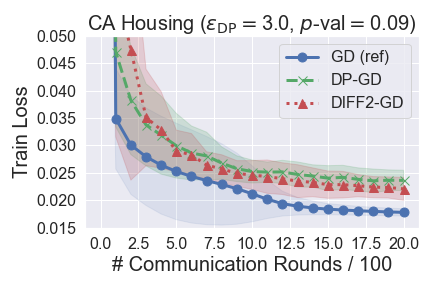
(a) Train Loss

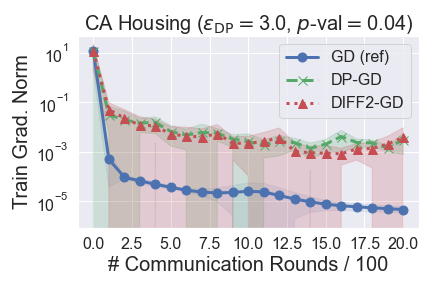
(b) Squared Train Grad. Norm

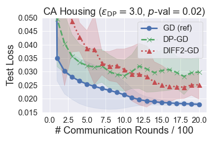
(c) Test Loss

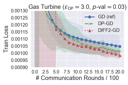
(d) Train Loss

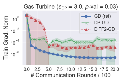
(e) Squared Train Grad. Norm

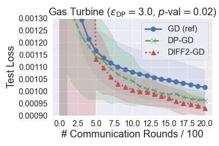
(f) Test Loss

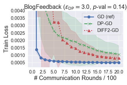
(g) Train Loss

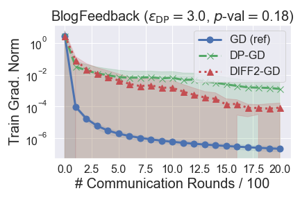
(h) Squared Train Grad. Norm

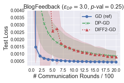
(i) Test Loss

Figure 1: Comparison of the train loss, train gradient norm and test loss against the number of communication rounds ($\varepsilon=3.0$, $\delta=10^{-5}$ and $R=2,000$). (a)-(c) shows the comparison of the three criteria on California Housing dataset, (d)-(f) do the ones on Gas Turbine CO and NOx Emission dataset and (g)-(i) do the ones on BlogFeedback dataset. DIFF2-GD consistently outperformed DP-GD.

Results. Figure 2 shows the comparison of DIFF2-GD with DP-GD on the three datasets for $\varepsilon_{\mathrm{DP}}=3.0$. “GD (ref)” means gradient descent without DP noise. “$p$-value” in the title of each figure means the $p$-value of the one-sided $t$-test with the alternative hypothesis that the difference of the minimum value in $2,000$ rounds of DIFF2-GD from the one of DP-GD is negative, where one random seed corresponded to one sample, i.e., the degree of freedom of $t$-distribution was four. We can observe that DIFF2-GD consistently outperformed DP-GD at the final learning rounds for each metric, although it sometimes showed slower convergence than DP-GD at initial learning rounds. Also, the results of $t$-test supported statistical significance of the superiority of DIFF2-GD. The case of $\varepsilon_{\mathrm{DP}}=5.0$ showed similar results to the case of $\varepsilon_{\mathrm{DP}}=3.0$, that are provided in the supplementary material due to the space limitation.

7 Conclusion and Future Work

In this work, we proposed a new differential private optimization framework called DIFF2 to improve the previous best known utility bound. DIFF2 communicates gradient differences rather than gradients themselves and constructs a differential private global gradient estimator with possibly quite small variance based on the gradient differences. It is shown that DIFF2 with a gradient descent subroutine achieves the utility of $\widetilde{O}(d^{2/3}/(n_{\mathrm{min}}P\varepsilon_{\mathrm{DP}})^{4/3})$, which can be significantly better than the previous one in terms of the dependence on sample size $n_{\mathrm{min}}P$. We conducted numerical experiments and confirmed the superiority of DIFF2-GD to DP-GD and the benefit of DIFF2 framework.

The first important future work is to derive a lower bound of the utility of $(\varepsilon_{\mathrm{DP}},\delta_{\mathrm{DP}})$-DP optimization algorithms for nonconvex smooth objectives and discuss the optimality of DIFF2 framework. The second important future work is to develop new utility analysis of DP optimization algorithms for high dimensional problems, which often arise in learning modern huge deep neural networks. While this work has tackled a quite fundamental and important problem, utility improvement, in DP optimization theory, our theoretical improvement is limited on relatively low dimensional problems. Finally, extensions of our algorithms to various directions are also important future work. For example, client sampling is typically used in cross-device FL, but is not discussed in this work. Also, DIFF2 framework on a decentralized topology is an important extension. It is non-trivial to extend our DP guarantees and utility analysis to these settings. While a more computational and communication efficient sub-routine than GD is briefly mentioned in Section 5, a broad range of optimization algorithms including simple SGD, accelerated gradient methods, adaptive gradient methods and so on can be incorporated into DIFF2 framework. Then, it is important to develop unified theoretical analysis and compare their theoretical and empirical performances.

Appendix A Supplementary Material for Numerical Experiments

In this section, we provide additional information and results on our numerical experiments that are not given in the main paper due to the space limitation.

Hyper-Parameter Tuning

The hyper-parameter of non-private GD was only learning rate $\eta$. The ones of DP-GD were learning rate $\eta$ and clipping radius $C_{1}$. The ones of Diff2-GD were learning rate $\eta$, the restart interval $T$ and clipping radius $C_{1}$ and $C_{2}$.

For tuning clipping radius and restart interval, we ran DP-GD with $C_{1}\in\{1,3.0,10.0,30.0,100.0\}$ and ran DIFF2-GD with $C_{1},C_{2}\in\{1,3.0,10.0,30.0,100.0\}$ and $T\in\{0.003R,0.01R,0.03R,0.1R\}$ for $2,000$ rounds. For tuning learning rate $\eta$, we ran each implemented algorithm with $\eta\in\{0.5^{i}|i\in\{0,\ldots,9\}\}$. To reduce the execution time, train loss was evaluated every $20$ rounds and the learning was stopped if the used learning rate was deemed inappropriate by checking the train loss. Specifically, the learning rate was determined to be inappropriate (i) if the train loss reached a NAN value; or (ii) if the patience count reached five. Here, the patience count was increased by one if the current train loss was greater than $1.05$ times the previous minimum train loss in the current learning, and reset to be zero if the current train loss was smaller than the previous best train loss. If we reached $2,000$ rounds using a certain learning rate $\eta_{*}$, the learning rate tuning was terminated and the best learning rate was determined to be $\eta_{*}$ instead of further trying smaller learning rates to avoid wasting computational resources.

For two criteria of train loss and squared train gradient norm, we chose the the best hyper-parameters that minimized the criteria and report the learning results with the best hyper-parameters. For test loss, we chose the the best hyper-parameters that minimized train loss and report the learning results with the best hyper-parameters.

These procedures were independently executed for all the five random seeds.

Datasets Information

The information of three datasets used in our experiments is summarized in Table 2.

Table 2: The summary of the datasets used in the numerical experiments.

Dataset	# Samples	# Attributes
California Housing	$20,640$	$8$
Gas Turbine CO and NOx Emission	$36,733$	$9$
BlogFeedback	$60,021$	$280$
Cover Type	$58,1012$	$54$
KDDCup99	$4,898,431$	$41$

Additional Numerical Results on Regression Tasks

Here, we provide additional numerical results on the case $\varepsilon_{\mathrm{DP}}=5.0$ on regression tasks. We confirmed that the results were similar to the ones when $\varepsilon_{\mathrm{DP}}=3.0$ provided in the main paper.

3 3 3

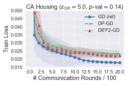
(a) Train Loss

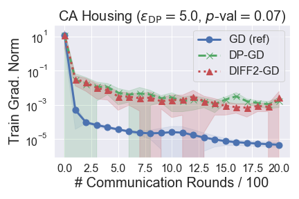
(b) Squared Train Grad. Norm

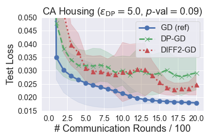
(c) Test Loss

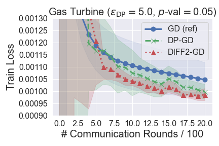
(d) Train Loss

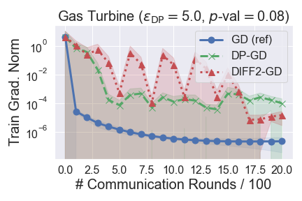
(e) Squared Train Grad. Norm

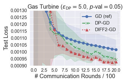
(f) Test Loss

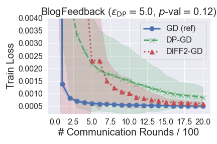
(g) Train Loss

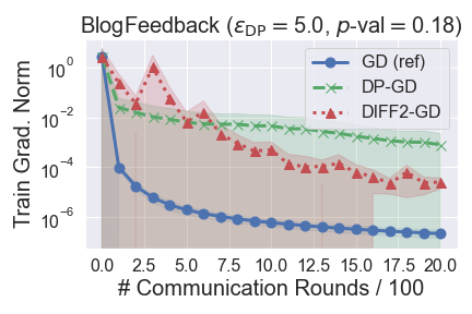
(h) Squared Train Grad. Norm

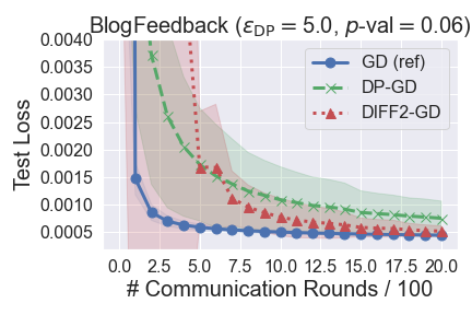
(i) Test Loss

Figure 2: Comparison of the train loss, train gradient norm and test loss against the number of communication rounds ($\varepsilon=5.0$, $\delta=10^{-5}$ and $R=2,000$). (a)-(c) shows the comparison of the three criteria on California Housing dataset, (d)-(f) do the ones on Gas Turbine CO and NOx Emission dataset and (g)-(i) do the ones on BlogFeedback dataset. We confirm that DIFF2-GD consistently outperformed DP-GD.

Computing Infrastructures

• OS: Ubuntu 16.04.6

• CPU: AMD EPYC 7552 48-Core Processor.

• CPU Memory: 1.0 TB.

• Programming language: Python 3.9.12.

• Deep learning framework: Pytorch 1.12.1.

Additional Numerical Results on Classification Tasks

Here, we provide additional numerical results on the case $\varepsilon_{\mathrm{DP}}=3.0$ on classification tasks. We confirm that the consistent superiority of the proposed method was observed even for classification tasks.

3 2 3 2

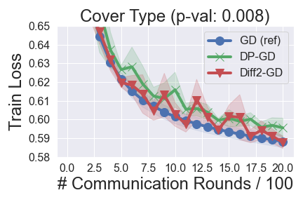
(a) Train Loss

(b) Squared Train Grad. Norm

(c) Train Acc

(d) Test Loss

(e) Test Acc

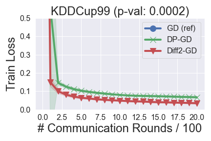
(f) Train Loss

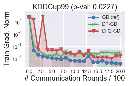
(g) Squared Train Grad. Norm

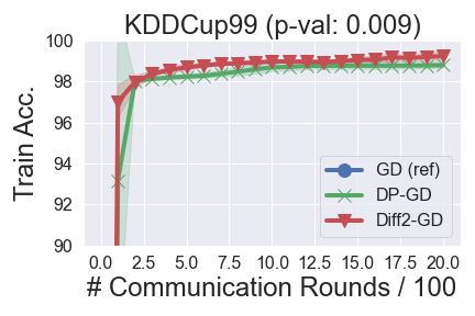
(h) Train acc

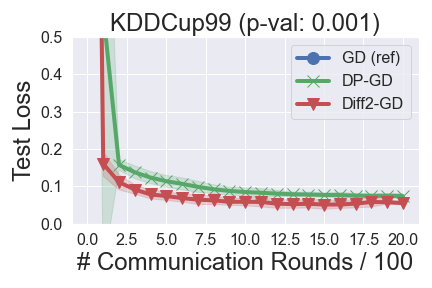
(i) Test Loss

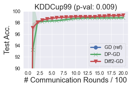
(j) Test Acc

Figure 3: Comparison of the train loss, train gradient norm and test loss against the number of communication rounds ($\varepsilon=3.0$, $\delta=10^{-5}$ and $R=2,000$). (a)-(e) shows the comparison of the three criteria on Cover Type dataset and (f)-(j) do the ones on KDDCup99 dataset. We confirm that DIFF2-GD consistently outperformed DP-GD.

Appendix B Review of Rényi Differential Privacy

Our DP analysis relies on Rényi differential privacy (RDP) technique with subsampling and shuffling amplification. In this section, we briefly review some known results about RDP used in our analysis.

Definition B.1 ($(\alpha,\varepsilon)$-RDP ((Mironov, 2017))).

A randomized mechanism $\mathcal{M}:\mathcal{D}\to\mathcal{R}$ satisfies $(\alpha,\varepsilon)$-RDP ($\alpha\in(1,\infty)$ and $\varepsilon>0$) if for any datasets $D,D^{\prime}\in\mathcal{D}$ with $d_{\mathrm{H}}(D,D^{\prime})=1$, it holds that

$$\frac{1}{\alpha-1}\log\mathbb{E}_{o\sim\mathcal{M}(D^{\prime})}\left(\frac{\mathcal{M}(D)(o)}{\mathcal{M}(D^{\prime})(o)}\right)^{\alpha}\leq\varepsilon,$$

where $M(D)(o)$ denotes the density of $\mathcal{M}(D)$ at $o$.

Lemma B.2 (Post-processing Property of RDP ((Mironov, 2017))).

Let $\mathcal{M}:\mathcal{D}\to\mathcal{R}$ be $(\alpha,\varepsilon)$-RDP and $g:\mathcal{R}\to\mathcal{R}^{\prime}$ be any function. Then, $g\circ\mathcal{M}:\mathcal{D}\to\mathcal{R}^{\prime}$ is also $(\alpha,\varepsilon)$-RDP.

Lemma B.3 (Composition of RDP Mechanisms ((Mironov, 2017))).

Let $\mathcal{M}_{r}:\mathcal{R}_{1}\times\cdots\times\mathcal{R}_{r-1}\times\mathcal{D}\to\mathcal{R}_{r}$ be $(\alpha,\varepsilon_{r})$-RDP for $r\in[R]$. Then, $\mathcal{M}:\mathcal{D}\to\mathcal{R}_{1}\times\cdots\times\mathcal{R}_{R}$ defined by $\mathcal{M}(D):=(\mathcal{M}_{1}(D),\mathcal{M}_{2}(\mathcal{M}_{1}(D),D),\ldots,\mathcal{M}_{R}(\mathcal{M}_{1}(D),\ldots,D))$ is $(\alpha,\sum_{r=1}^{R}\varepsilon_{r})$-RDP.

Lemma B.4 (From RDP to DP ((Mironov, 2017))).

If a randomized mechanism $\mathcal{M}$ is $(\alpha,\varepsilon)$-RDP, then $\mathcal{M}$ is $(\varepsilon+\log(1/\delta)/(\alpha-1),\delta)$-DP for every $\delta\in(0,1)$.

Definition B.5 ($l_{q}$-sensitivity).

$\Delta_{q}(h):=\sup_{d_{\mathrm{H}}(D,D^{\prime})=1}\|h(D)-h(D^{\prime})\|_{q}$ is called $l_{q}$-sensitivity for function $h$, where the maximum is taken over any adjacent datasets $D,D^{\prime}\in\mathcal{D}$.

Lemma B.6 (Gaussian Mechanism ((Mironov, 2017))).

Given a function $h$, Gaussian Mechanism $\mathcal{M}(D):=h(D)+\mathcal{N}(0,\sigma_{1}^{2}I)$ satisfies $(\alpha,\alpha\Delta_{2}^{2}(h)/(2\sigma_{1}^{2}))$-RDP for every $\alpha\in(1,\infty)$.

Lemma B.7 (Subsampling Amplification (Theorem 9 in (Wang et al., 2019c))).

Let $\mathcal{M}$ be a randomized mechanism that takes a dataset of $b\leq n$ points as an input and $\gamma:=b/n$. $\mathcal{M}\circ\mathrm{subsample}_{\gamma}$ be defined as: (1) $\mathrm{subsample}_{\gamma}$: subsample $\gamma n$ points without replacement from the input dataset with size $n$, and (2) apply $\mathcal{M}$ taking the subsampled points as the input. For every integer $\alpha\geq 2$, if $\mathcal{M}$ is $(\alpha,\varepsilon(\alpha))$-RDP, $\mathcal{M}\circ\mathrm{subsample}_{\gamma}$ is $(\alpha,\varepsilon^{\prime}(\alpha))$-RDP, where

$$\varepsilon^{\prime}(\alpha)\leq \ \frac{1}{\alpha-1}\log\left(1+\gamma^{2}\binom{\alpha}{2}\min\left\{4(e^{\varepsilon(2)}-1),e^{\varepsilon(2)}\min\{2,(e^{\varepsilon(\infty)}-1)^{2}\}\right\}\right.$$

$$+\left.\sum_{j=3}^{\alpha}\gamma^{j}\binom{\alpha}{j}e^{(j-1)\varepsilon(j)}\min\{2,(e^{\varepsilon(\infty)}-1)^{j}\}\right).$$

We can derive a simple upper bound using Lemma B.7.

Lemma B.8 (Subsampling Amplification (Simple Upper Bound)).

On the same settings as in Lemma B.7, if $\varepsilon(\alpha)$ is monotonically increasing with respect to $\alpha$, it holds that

$$\varepsilon^{\prime}(\alpha)\leq \ \frac{2}{3}\left(4+\frac{e}{c}\right)\frac{\gamma^{2}\alpha^{2}\varepsilon(2)}{\alpha-1}$$

under $\varepsilon(\alpha)\leq 1/3\wedge\log(1/(2\gamma\alpha))$ and $\gamma\leq\varepsilon(2)/(c\alpha)$ for some $c>0$.

Proof.

From Lemma B.7, we have

$$\varepsilon^{\prime}(\alpha)\leq \ \frac{1}{\alpha-1}\log\left(1+4\gamma^{2}\binom{\alpha}{2}(e^{\varepsilon(2)}-1)+2\sum_{j=3}^{\alpha}\gamma^{j}\binom{\alpha}{j}e^{(j-1)\varepsilon(j)}\right).$$

Suppose that $\varepsilon(\alpha)\leq\log(1/(2\gamma\alpha))$. Then, we can see that $\gamma\alpha e^{\varepsilon(\alpha)}<1/2$. The third term can be bounded as follows:

$$2\sum_{j=3}^{\alpha}\gamma^{j}\binom{\alpha}{j}e^{(j-1)\varepsilon(j)}\leq \ \frac{1}{3}\sum_{j=3}^{\alpha}(\gamma\alpha e^{\varepsilon(\alpha)})^{j}$$

$$\leq \ \frac{1}{3}\frac{(\gamma\alpha e^{\varepsilon(\alpha)})^{3}}{1-\gamma\alpha e^{\varepsilon(\alpha)}}$$

$$\leq \ \frac{2(\gamma\alpha e^{\varepsilon(\alpha)})^{3}}{3}$$

Assume that $\gamma\leq\varepsilon(2)/(c\alpha)$ for some $c>0$. Then, we have

$$2\sum_{j=3}^{\alpha}\gamma^{j}\binom{\alpha}{j}e^{(j-1)\varepsilon(j)}\leq \ \frac{2\gamma^{2}\alpha^{2}e^{3\varepsilon(\alpha)}\varepsilon(2)}{3c}.$$

Hence, we obtain

$$\varepsilon^{\prime}(\alpha)\leq \ \frac{1}{\alpha-1}\log\left(1+\left(2(e^{\varepsilon(2)}-1)+\frac{2e^{3\varepsilon(\alpha)}\varepsilon(2)}{3c}\right)\gamma^{2}\alpha^{2}\right)$$

$$\leq \ \left(2(e^{\varepsilon(2)}-1)+\frac{2e^{3\varepsilon(\alpha)}\varepsilon(2)}{3c}\right)\frac{\gamma^{2}\alpha^{2}}{\alpha-1}$$

$$\leq \ \left(2\varepsilon(2)(1+\varepsilon(2))+\frac{2e\varepsilon(2)}{3c}\right)\frac{\gamma^{2}\alpha^{2}}{\alpha-1}.$$

Here, for the second inequality, we used $\log(1+x)\leq x$. The last inequality holds because $e^{x}-1\leq x+x^{2}$ for $x\leq 3/2$ by assuming $\varepsilon(2)\leq\varepsilon(\alpha)\leq 1/3\leq 3/2$. This gives the desired result. ∎

Appendix C Differential Privacy Analysis of DIFF2-GD

In this section, we investigate differential privacy level of DIFF2 (Algorithm 1) with GD-Routine (Algorithm 3).

First, we consider the $l_{2}$-sensitivity of $v_{r}$ for $r\in[R]$ with respect to $D_{p}$.

Lemma C.1 ($l_{2}$-Sensitivity of $v_{r}$).

In Algorithm 1, $v_{1}$ has $l_{2}$-sensitivity $2C_{1}/(n_{p}P)$ with respect to $D_{p}$. Furthermore, given the outputs of the previous mechanisms $\{x_{r^{\prime}},\widetilde{v}_{r^{\prime}}\}_{r^{\prime}\in[r-1]}$, $v_{r}$ has $l_{2}$-sensitivity $2C_{2,r}/(n_{p}P)$ with respect to $D_{p}$.

Proof.

When $(r-1)\%T=0$, the $l_{2}$-sensitivity of $v_{1}=(1/P)\sum_{p=1}^{P}d_{1}^{(p)}$ for adjacent local datasets $D_{p}$ and $D_{p}^{\prime}$ can be bounded as

$$\frac{1}{n_{p}P}\left\|\min\left\{\frac{C_{1}}{\|\nabla\ell(x_{r-1},z)\|},1\right\}\nabla\ell(x_{r-1},z)-\min\left\{\frac{C_{1}}{\|\nabla\ell(x_{r-1},z^{\prime})\|},1\right\}\nabla\ell(x_{r-1},z^{\prime})\right\|\leq\frac{2C_{1}}{n_{p}P}$$

for some $z\neq z^{\prime}$ from the definition of $d_{1}^{(p)}$ since $x_{r-1}$ is fixed.

When $(r-1)\%T\neq 0$, the $l_{2}$-sensitivity of $v_{r}=(1/P)\sum_{p=1}^{P}d_{r}^{(p)}+\widetilde{v}_{r-1}$ for adjacent local datasets $D_{p}$ and $D_{p}^{\prime}$ can be bounded as

$$\frac{1}{n_{p}P}\left\|\min\left\{\frac{C_{2,r}}{\|\nabla\ell(x_{r-1},z)-\nabla\ell(x_{r-2},z)\|},1\right\}(\nabla\ell(x_{r-1},z)-\nabla\ell(x_{r-2},z)\right.$$

$$-\left.\min\left\{\frac{C_{2,r}}{\|\nabla\ell(x_{r-1},z^{\prime})-\nabla\ell(x_{r-2},z^{\prime})\|},1\right\}(\nabla\ell(x_{r-1},z^{\prime})-\nabla\ell(x_{r-2},z^{\prime})\right\|\leq\frac{2C_{2,r}}{n_{p}P}$$

for some $z\neq z^{\prime}$ from the definition of $d_{r}^{(p)}$ since $x_{r-1}$, $x_{r-2}$ and $\widetilde{v}_{r-1}$ are fixed. This finishes the proof. ∎

Combined Lemma C.1 with Lemmas B.6 and B.3, we can show Proposition 4.1.

Proof of Proposition 4.1

First, we derive a RDP bound with respect to $D_{p}$ for each mechanism $\widetilde{v}_{k,r}$.

When $(r-1)\%T=0$, from Lemma B.6, we know that $\widetilde{v}_{r}$ is $(\alpha,2\alpha/(n_{p}^{2}P^{2}\sigma_{1}^{2}))$-RDP for every $\alpha\in(1,\infty)$ since $\xi_{1}\sim\mathcal{N}(0,\sigma_{1}^{2}C_{1}^{2}I)$ and $v_{1}$ has $l_{2}$-sensitivity $\Delta_{2}=2C_{1}/(n_{p}P)$ by the first part of Lemma C.1.

Similarly, when $(r-1)\%T\neq 0$, from Lemma B.6, we know that $\widetilde{v}_{r}$ is $(\alpha,2\alpha/(n_{p}^{2}P^{2}\sigma_{2}^{2}))$-RDP for every $\alpha\in(1,\infty)$ since $\xi_{r}\sim\mathcal{N}(0,\sigma_{2}^{2}C_{2,r}^{2}I)$ and $v_{r}$ has $l_{2}$-sensitivity $\Delta_{2}=2C_{2,r}/(n_{p}P)$ by the second part of Lemma C.1.

Hence, given $\{x_{r^{\prime}},x_{r^{\prime}}^{\mathrm{out}},\widetilde{v}_{r^{\prime}}\}_{r^{\prime}\in[r-1]}$, $\{x_{r},x_{r}^{\mathrm{out}},\widetilde{v}_{r}\}$ are $(\alpha,2\alpha/(n_{p}^{2}P^{2}\sigma^{2}))$-RDP from the post-processing property of RDP (Lemma B.2) since $x_{r}=x_{r}^{\mathrm{out}}=x_{r-1}-\eta\widetilde{v}_{r}$, where $\sigma^{2}=\sigma_{1}^{2}$ when $(r-1)\%T=0$ and $\sigma^{2}=\sigma_{2}^{2}$ when $(r-1)\%T\neq 0$.

Now, by Lemma B.3, it holds that mechanism $\{x_{r},x_{r}^{\mathrm{out}},\widetilde{v}_{r}\}_{r\in[R]}$ is $(\alpha,2\alpha\lceil R/T\rceil/(n_{p}^{2}P^{2}\sigma_{1}^{2})+2\alpha(R-\lceil R/T\rceil)/(n_{p}^{2}P^{2}\sigma_{2}^{2}))$-RDP with respect to $D_{p}$.

Therefore, setting $\alpha=1+\lceil 2\log(1/\delta_{\mathrm{DP}})/\varepsilon_{\mathrm{DP}}\rceil$, we only need to find $\sigma_{1}^{2}$ and $\sigma_{2}^{2}$ that satisfy $2\alpha\lceil R/T\rceil/(n_{p}^{2}P^{2}\sigma_{1}^{2})+2\alpha(R-\lceil R/T\rceil)/(n_{p}^{2}P^{2}\sigma_{2}^{2}))\leq\varepsilon/2$. Then, we can see that for any constant $u>1$, it is sufficient that $\sigma_{1}^{2}=4u\alpha\lceil R/T\rceil/(n_{\mathrm{min}}^{2}P^{2}\varepsilon_{\mathrm{DP}})$ and $\sigma_{2}^{2}=(4u/(u-1))\alpha(R-\lceil R/T\rceil)/(n_{\mathrm{min}}^{2}P^{2}\varepsilon_{\mathrm{DP}})$ guarantees $(\varepsilon_{\mathrm{DP}},\delta_{\mathrm{DP}})$-DP of mechanism $\{x_{r},x_{r}^{\mathrm{out}},\widetilde{v}_{r}\}_{r\in[R]}$. This is the desired result.

Appendix D Utility Analysis of DIFF2-GD

In this section, we give utility analysis of DIFF2 (Algorithm 1) with GD-Routine (Algorithm 3).

Lemma D.1 (Descent Lemma).

Suppose that Assumption 2.1 holds. Under $\eta\leq 1/(2L)$, DIFF2 (Algorithm 1) satisfies

$$\mathbb{E}[f(x_{r})]\leq \ \mathbb{E}[f(x_{r-1})]-\frac{\eta}{2}\mathbb{E}\|\nabla f(x_{r-1})\|^{2}-\frac{1}{4\eta}\mathbb{E}\|x_{r}-x_{r-1}\|^{2}$$

$$+\eta\mathbb{E}\left\|\frac{1}{\eta}(x_{r-1}-x_{r})-\nabla f(x_{r-1})\right\|^{2}.$$

for every round $r\in[R]$.

Proof.

From $L$-smoothness of $f$, we have

$$f(x_{r})\leq \ f(x_{r-1})+\langle\nabla f(x_{r-1}),x_{r}-x_{r-1}\rangle+\frac{L}{2}\|x_{r}-x_{r-1}\|^{2}$$

$$= \ f(x_{r-1})+\frac{1}{\eta}\left(-\frac{\eta^{2}}{2}\|\nabla f(x_{r-1})\|^{2}-\frac{1}{2}\|x_{r}-x_{r-1}\|^{2}+\frac{1}{2}\|x_{r}-x_{r-1}+\eta\nabla f(x_{r-1})\|^{2}\right)$$

$$+\frac{L}{2}\|x_{r}-x_{r-1}\|^{2}$$

$$= \ f(x_{r-1})-\frac{\eta}{2}\|\nabla f(x_{r-1})\|^{2}-\left(\frac{1}{2\eta}-\frac{L}{2}\right)\|x_{r}-x_{r-1}\|^{2}+\frac{\eta}{2}\left\|\frac{1}{\eta}(x_{r-1}-x_{r})-\nabla f(x_{r-1})\right\|^{2}.$$

Taking expectation on both sides with respect to all the history of the randomness and assuming $\eta\leq 1/(2L)$ yield the desired result. ∎

Proposition D.2.

Suppose that Assumption 2.1, 2.2 and 2.3 hold. Assume that $C_{1}\geq G$ and $C_{2}\geq L$. Then, if we appropriately choose $\eta=\Theta(\min\{1/L,1/\sqrt{T\sigma_{2}^{2}C_{2}^{2}d}\}$, DIFF2-GD satisfies

$$\mathbb{E}\|\nabla f(x^{\mathrm{out}})\|^{2}\leq \ O\left(\frac{f(x_{0})-f(x_{*})}{\eta R}+\sigma_{1}^{2}C_{1}^{2}d\right).$$

Proof.

Averaging the inequality in Lemma D.1 from $r=1$ to $R$, we know that

$$\mathbb{E}\|\nabla f(x^{\mathrm{out}})\|^{2}=\frac{1}{R}\sum_{r=1}^{R}\mathbb{E}\|\nabla f(x_{r-1})\|^{2}\leq \ \frac{2(f(x_{0})-f(x_{*}))}{\eta R}-\frac{1}{2\eta^{2}}\frac{1}{R}\sum_{r=1}^{R}\mathbb{E}\|x_{r}-x_{r-1}\|^{2}$$

$$+\frac{2}{R}\sum_{r=1}^{R}\mathbb{E}\left\|\frac{1}{\eta}(x_{r-1}-x_{r})-\nabla f(x_{r-1})\right\|^{2}.$$ (1)

Here, we used the existence of optimal solution $x_{*}$.

Now, we consider the last term in (1). Since $x_{r}-x_{r-1}=-\eta\widetilde{v}_{r}$, we have

$$\left\|\frac{1}{\eta}(x_{r-1}-x_{r})-\nabla f(x_{r-1})\right\|^{2}=\|\widetilde{v}_{r}-\nabla f(x_{r-1})\|^{2}.$$

First, we consider the case $(r-1)\%T=0$. Since $C_{1}\geq G$ is assumed, it holds that $(1/P)\sum_{p=1}^{P}d_{r}^{(p)}=\nabla f(x_{r-1})$ and thus $\widetilde{v}_{r}=\nabla f(x_{r-1})+\xi_{r}$. Then, we have

$$\mathbb{E}\|\widetilde{v}_{r}-\nabla f(x_{r-1})\|^{2}= \ \mathbb{E}\|\xi_{r}\|^{2}=\sigma_{1}^{2}C_{1}^{2}d.$$

Next, we consider the case $(r-1)\%T\neq 0$. Since $C_{2}\geq L$ is assumed, it holds that $(1/P)\sum_{p=1}^{P}d_{r}^{(p)}=\nabla f(x_{r-1})-\nabla f(x_{r-2})$ and thus $\widetilde{v}_{r}=\nabla f(x_{r-1})-\nabla f(x_{r-2})+\widetilde{v}_{r-1}+\xi_{r}$. Then, observe that

$$\mathbb{E}\|\widetilde{v}_{r}-\nabla f(x_{r-1})\|^{2}= \ \mathbb{E}\|\widetilde{v}_{r-1}-\nabla f(x_{r-2})+\xi_{r}\|^{2}$$

$$= \ \mathbb{E}\|\widetilde{v}_{r-1}-\nabla f(x_{r-2})\|^{2}+\mathbb{E}\|\xi_{r}\|^{2}$$

$$= \ \sum_{r^{\prime}=T(r)}^{r}\mathbb{E}\|\xi_{r^{\prime}}\|^{2}$$

$$= \ \sigma_{1}^{2}C_{1}^{2}d+\sigma_{2}^{2}d\sum_{r^{\prime}=T(r)+1}^{r}C_{2,r}^{2},$$

where $T(r)$ is the integer that satisfies $r+1-T\leq T(r)<r$ and $(T(r)-1)\%T=0$. Here, we used the fact that $\widetilde{v}_{T(r)}=\nabla f(x_{T(r)-1})+\xi_{T(r)}$. Using this relation, we get

$$\frac{1}{R}\sum_{r=1}^{R}\mathbb{E}\|\widetilde{v}_{r}-\nabla f(x_{r-1})\|^{2}= \ \sigma_{1}^{2}C_{1}^{2}d+\sigma_{2}^{2}C_{2}^{2}d\frac{1}{R}\sum_{r=1}^{R}\sum_{r=T(r)+1}^{r}\|x_{r-1}-x_{r-2}\|^{2}$$

$$\leq \ \sigma_{1}^{2}C_{1}^{2}d+\sigma_{2}^{2}C_{2}^{2}d\frac{1}{R}\sum_{r=1}^{R}\sum_{r=T(r)}^{T(r)+T-1}\|x_{r-1}-x_{r-2}\|^{2}$$

$$\leq \ \sigma_{1}^{2}C_{1}^{2}d+T\sigma_{2}^{2}C_{2}^{2}d\frac{1}{R}\sum_{r=1}^{R}\|x_{r-1}-x_{r-2}\|^{2}.$$

Suppose that $\eta\leq 1/(2\sqrt{T\sigma_{2}^{2}C_{2}^{2}d})$. Then, it holds that

$$-\frac{1}{2\eta^{2}}\frac{1}{R}\sum_{r=1}^{R}\mathbb{E}\|x_{r}-x_{r-1}\|^{2}+\frac{2}{R}\sum_{r=1}^{R}\mathbb{E}\left\|\frac{1}{\eta}(x_{r-1}-x_{r})-\nabla f(x_{r-1})\right\|^{2}\leq 2\sigma_{1}^{2}C_{1}^{2}d.$$

Applying this to (1), we obtain

$$\mathbb{E}\|\nabla f(x^{\mathrm{out}})\|^{2}\leq \ O\left(\frac{f(x_{0})-f(x_{*})}{\eta R}+\sigma_{1}^{2}C_{1}^{2}d\right).$$

This is the desired result. ∎

Proof of Theorem 4.3

From Proposition D.2, under $C_{1}=\Theta(G)$, we know that

$$\mathbb{E}\|\nabla f(x^{\mathrm{out}})\|^{2}\leq \ O\left(\frac{f(x_{0})-f(x_{*})}{\eta R}+\sigma_{1}^{2}G^{2}d\right).$$

Suppose that $f(x_{0})-f(x_{*})=O(1)$.

By Proposition 4.1, the necessary noise levels for $(\varepsilon_{\mathrm{DP}},\delta_{\mathrm{DP}})$-DP with respect to $D_{p}$ is $\sigma_{1}^{2}=\widetilde{\Theta}(R/(Tn_{\mathrm{min}}^{2}P^{2}\varepsilon_{\mathrm{DP}}^{2}))$ and $\sigma_{2}^{2}=\widetilde{\Theta}(R/(n_{\mathrm{min}}^{2}P^{2}\varepsilon_{\mathrm{DP}}^{2}))$ respectively. Using these results and substituting the definition of $\eta$, we have

$$\mathbb{E}\|\nabla f(x^{\mathrm{out}})\|^{2}\leq \ O\left(\frac{1}{\eta R}\right)+\widetilde{O}\left(\frac{RG^{2}d}{Tn_{\mathrm{min}}^{2}P^{2}\varepsilon_{\mathrm{DP}}^{2}}\right)$$

$$= \ O\left(\frac{L+\sqrt{T}L\sigma_{2}\sqrt{d}}{R}\right)+\widetilde{O}\left(\frac{RG^{2}d}{Tn_{\mathrm{min}}^{2}P^{2}\varepsilon_{\mathrm{DP}}^{2}}\right)$$

$$= \ O\left(\frac{L}{R}\right)+\widetilde{O}\left(\frac{\sqrt{T}L\sqrt{d}}{n_{\mathrm{min}}P\varepsilon_{\mathrm{DP}}\sqrt{R}}+\frac{RG^{2}d}{Tn_{\mathrm{min}}^{2}P^{2}\varepsilon_{\mathrm{DP}}^{2}}\right).$$

Assume that $n_{\mathrm{min}}P=\Omega(G^{2}\sqrt{d}/(L\varepsilon_{\mathrm{DP}}))$. We define

$$T:=\Theta\left(1\vee\left(\frac{G^{2}\sqrt{d}}{Ln_{\mathrm{min}}P\varepsilon_{\mathrm{DP}}}\right)^{\frac{2}{3}}R\right)$$

with $1\leq T\leq R$.

Then, we obtain

$$\mathbb{E}\|\nabla f(x^{\mathrm{out}})\|^{2}\leq \ O\left(\frac{L}{R}\right)+\widetilde{O}\left(\frac{L\sqrt{d}}{n_{\mathrm{min}}P\varepsilon_{\mathrm{DP}}\sqrt{R}}+\frac{(LGd)^{\frac{2}{3}}}{(n_{\mathrm{min}}P\varepsilon_{\mathrm{DP}})^{\frac{4}{3}}}\right).$$

Finally, setting

$$R=\Theta\left(1\vee\frac{L}{\varepsilon_{\mathrm{opt}}}\right)\vee\widetilde{\Theta}\left(\frac{L^{2}d}{n_{\mathrm{min}}^{2}P^{2}\varepsilon_{\mathrm{DP}}^{2}\varepsilon_{\mathrm{opt}}^{2}}\right)$$

with $\varepsilon_{\mathrm{opt}}:=\Theta\left(\frac{(LGd)^{\frac{2}{3}}}{(n_{\mathrm{min}}P\varepsilon_{\mathrm{DP}})^{\frac{4}{3}}}\right)$ gives the desired result.

Appendix E Differential Privacy Analysis of DIFF2-BVR-L-SGD

In this section, we provide differential privacy analysis of DIFF2 (Algorithm 1) with BVR-L-SGD-Routine (Algorithm 4). We investigate the minimum noise level $\sigma_{1}^{2}$, $\sigma_{2}^{2}$ and $\sigma_{3}^{2}$ to satisfy $(\varepsilon_{\mathrm{DP}},\delta_{\mathrm{DP}})$-DP with respect to $D_{p}$ for $p\in[P]$.

Since we can utilize Lemma C.1 for the $l_{2}$ sensitivity of $v_{r}$, we focus on the $l_{2}$-sensitivity of $v_{k,r}$ for $k\in[K]$ and $r\in[R]$.

Lemma E.1 ($l_{2}$-Sensitivity of $v_{k,r}$).

Given the outputs of the previous mechanisms $\{x_{r-1},\widetilde{v}_{r}\}\cup\{x_{k^{\prime},r-1}\}_{k^{\prime}\in[k-1]}$, the $l_{2}$-sensitivity of $v_{k,r}$ defined in Algorithm 4 is

$$\begin{cases}\frac{2C_{3,k,r}}{b}&(p=p_{r}),\\ 0&(p\neq p_{r}).\end{cases}$$

with respect to $D_{p}$ for $k\geq 2$.

Proof.

The $l_{2}$-sensitivity of $v_{k,r}$ for adjacent local datasets $D_{p}$ and $D_{p}^{\prime}$ can be bounded as

$$\frac{1}{b}\left\|\min\left\{\frac{C_{3,k,r}}{\|\nabla\ell(x_{k-1,r-1},z)-\nabla\ell(x_{k-2,r-1},z)\|},1\right\}(\nabla\ell(x_{k-1,r-1},z)-\nabla\ell(x_{k-2,r-1},z)\right.$$

$$-\left.\min\left\{\frac{C_{3,k,r}}{\|\nabla\ell(x_{k-1,r-1},z^{\prime})-\nabla\ell(x_{k-2,r-1},z^{\prime})\|},1\right\}(\nabla\ell(x_{k-1,r-1},z^{\prime})-\nabla\ell(x_{k-2,r-1},z^{\prime})\right\|\leq\frac{2C_{3,k,r}}{b}$$

for some $z\neq z^{\prime}$ from the definition of $v_{k,r}^{(p)}$ since $x_{k-1,r-1}$, $x_{k-2,r-1}$ and $\widetilde{v}_{k-1,r}$ are fixed. When $p\neq p_{r}$, the sensitivity of $v_{k,r}$ with respect to $p$ is trivially zero. This finishes the proof. ∎

Combined Lemmas C.1 and E.1 with Lemmas B.6 and B.3, we have the following Proposition:

Proposition E.2 (Minimum Noise Level for $(\varepsilon_{\mathrm{DP}},\delta_{\mathrm{DP}})$-DP).

For every integer $\alpha\geq 2$, mechanism $\{x_{r},x_{r}^{\mathrm{out}},\widetilde{v}_{r}\}_{r\in[R]}$ defined in DIFF2-BVR-L-SGD is $(2\alpha\lceil R/T\rceil/(n_{p}^{2}P^{2}\sigma_{1}^{2})+2\alpha(R-\lceil R/T\rceil)/(n_{p}^{2}P^{2}\sigma_{2}^{2})+K\lceil R/P\rceil\varepsilon^{\prime}(\alpha)+\log(1/\delta_{\mathrm{DP}})/(\alpha-1),\delta_{\mathrm{DP}})$-DP, where $\varepsilon^{\prime}(\alpha)$ is defined in Lemma B.7 with $\varepsilon(\alpha):=2\alpha/(b^{2}\sigma_{3}^{2})$ and $n_{\mathrm{min}}:=\min\{n_{p}\}_{p=1}^{P}$. In particular, setting $\alpha:=1+\lceil 2\log(1/\delta_{\mathrm{DP}})/\varepsilon_{\mathrm{DP}}\rceil$,

$$\sigma_{1}^{2}=\frac{4u_{1}\alpha\lceil\frac{R}{T}\rceil}{n_{\mathrm{min}}^{2}P^{2}\varepsilon_{\mathrm{DP}}}\text{, }\sigma_{2}^{2}=\frac{4u_{2}\alpha(R-\lceil\frac{R}{T}\rceil)}{n_{\mathrm{min}}^{2}P^{2}\varepsilon_{\mathrm{DP}}}\text{ and }2K\left\lceil\frac{R}{P}\right\rceil\varepsilon^{\prime}(\alpha)\leq\left(1-\frac{1}{u_{1}}-\frac{1}{u_{2}}\right)\varepsilon_{\mathrm{DP}}$$

are a sufficient condition to guarantee $(\varepsilon_{\mathrm{DP}},\delta_{\mathrm{DP}})$-DP for any constants $u_{1},u_{2}>1$.

Furthermore, there exist $\sigma_{1}^{2}$, $\sigma_{2}^{2}$ and $\sigma_{3}^{2}$ which satisfy the above condition such that

$$\sigma_{1}^{2}=\widetilde{\Theta}\left(\frac{R}{Tn_{\mathrm{min}}^{2}P^{2}\varepsilon_{\mathrm{DP}}^{2}}\right)\text{, }\sigma_{2}^{2}=\widetilde{\Theta}\left(\frac{R}{n_{\mathrm{min}}^{2}P^{2}\varepsilon_{\mathrm{DP}}^{2}}\right)\text{ and }\sigma_{3}^{2}=\widetilde{\Theta}\left(\frac{KR}{n_{\mathrm{min}}^{2}P\varepsilon_{\mathrm{DP}}^{2}}\vee\frac{1}{b^{2}\varepsilon_{\mathrm{DP}}}\right)$$

under $b\leq\min\{n_{\mathrm{min}}/(2e\alpha),(4n_{\mathrm{min}}/(\alpha\sigma_{3}^{2}))^{1/3}\}$.

Proof.

First, from the arguments of Lemma C.1, we know that $\widetilde{v}_{1,r}=\widetilde{v}_{r}$ and thus $x_{1,r-1}$ is $(\alpha,2\alpha/(n_{p}^{2}P^{2}\sigma_{1}^{2}))$-RDP when $(r-1)\%T=0$ and $(\alpha,2\alpha/(n_{p}^{2}P^{2}\sigma_{2}^{2}))$-RDP when $(r-1)\%T\neq 0$ for every $\alpha\in(1,\infty)$ given the outputs of the previous mechanisms.

Next, if $p=p_{r}$, from Lemmas B.6 and E.1, given a subsampled minibatch, it holds that $\widetilde{v}_{k,r}$ is $(\alpha,\varepsilon(\alpha))$-RDP for $k\geq 2$, where $\varepsilon(\alpha):=2\alpha/(b^{2}\sigma_{3}^{2})$ for every $\alpha\in(1,\infty)$ since $\xi_{2,r}\sim\mathcal{N}(0,\sigma_{3}^{2}C_{3,k,r}^{2}I)$. Then, applying Lemma B.7, we can see that $\widetilde{v}_{k,r}$ is $(\alpha,\varepsilon^{\prime}(\alpha))$-RDP for integer $\alpha\geq 2$, where $\varepsilon^{\prime}(\alpha)$ is defined in Lemma B.7 given the outputs of the previous mechanisms. This implies that $\{x_{k,r-1},\widetilde{v}_{k,r}\}$ is also $(\alpha,\varepsilon^{\prime}(\alpha))$-RDP for $k\geq 2$ from Lemma B.2 given the outputs of the previous mechanisms.

When $p\neq p_{r}$, $\widetilde{v}_{k,r}$ and thus $x_{k,r-1}$ are trivially $(\alpha,0)$-RDP with respect to $D_{p}$ for $k\geq 2$.

Now, by Lemma B.3, it holds that mechanism $\{x_{k,r-1}\}_{k\in[K]\cup\{0\},r\in[R]}\cup\{\widetilde{v}_{k,r}\}_{k\in[K],r\in[R]}$ is $(\alpha,2\alpha\lceil R/T\rceil/(n_{p}^{2}P^{2}\sigma_{1}^{2})+2\alpha(R-\lceil R/T\rceil)/(n_{p}^{2}P^{2}\sigma_{2}^{2})+K\lceil R/P\rceil\varepsilon^{\prime}(\alpha))$-RDP with respect to $D_{p}$.

Then, using Lemma B.4, we can see that mechanism $\{x_{k,r-1}\}_{k\in[K]\cup\{0\},r\in[R]}\cup\{\widetilde{v}_{k,r}\}_{k\in[K],r\in[R]}$ is $(2\alpha\lceil R/T\rceil/(n_{p}^{2}P^{2}\sigma_{1}^{2})+2\alpha(R-\lceil R/T\rceil)/(n_{p}^{2}P^{2}\sigma_{2}^{2})+K\lceil R/P\rceil\varepsilon^{\prime}(\alpha)+\log(1/\delta_{\mathrm{DP}})/(\alpha-1),\delta_{\mathrm{DP}})$-DP for every integer $\alpha\geq 2$. Note that $\{x_{r},x_{r}^{\mathrm{out}},\widetilde{v}_{r}\}_{r\in[R]}\subset\{x_{k,r-1}\}_{k\in[K]\cup\{0\},r\in[R]}\cup\{\widetilde{v}_{k,r}\}_{k\in[K],r\in[R]}$.

Now, choosing $\alpha:=1+\lceil 2\log(1/\delta_{\mathrm{DP}})/\varepsilon_{\mathrm{DP}}\rceil$,

$$\sigma_{1}^{2}=\frac{4u_{1}\alpha\lceil\frac{R}{T}\rceil}{n_{\mathrm{min}}^{2}P^{2}\varepsilon_{\mathrm{DP}}}=\widetilde{\Theta}\left(\frac{R}{Tn_{\mathrm{min}}^{2}P^{2}\varepsilon_{\mathrm{DP}}^{2}}\right),$$

$$\sigma_{2}^{2}=\frac{4u_{2}\alpha(R-\lceil\frac{R}{T}\rceil)}{n_{\mathrm{min}}^{2}P^{2}\varepsilon_{\mathrm{DP}}}=\widetilde{\Theta}\left(\frac{R}{n_{\mathrm{min}}^{2}P^{2}\varepsilon_{\mathrm{DP}}^{2}}\right),$$

and

$$2K\left\lceil\frac{R}{P}\right\rceil\varepsilon^{\prime}(\alpha)\leq\left(1-\frac{1}{u_{1}}-\frac{1}{u_{2}}\right)\varepsilon_{\mathrm{DP}}$$

guarantees $(\varepsilon_{\mathrm{DP}},\delta_{\mathrm{DP}})$ of mechanism $\{x_{r},x_{r}^{\mathrm{out}},\widetilde{v}_{r}\}_{r\in[R]}$ for any constants $u_{1},u_{2}>1$.

Finally, we derive a simple upper bound of $\sigma_{3}^{2}$. From Lemma B.8, we know that

$$\varepsilon^{\prime}(\alpha)\leq \ \frac{2}{3}\left(4+e\right)\frac{\gamma^{2}\alpha^{2}\varepsilon(2)}{\alpha-1}$$

under $\varepsilon(\alpha)\leq 1/3\wedge\log(1/(2\gamma\alpha))$ and $\gamma\leq\varepsilon(2)/\alpha$.

Suppose that

$$\sigma_{3}^{2}\geq\frac{8}{3}\left(4+e\right)\frac{\alpha^{2}}{\alpha-1}\frac{6K\lceil\frac{R}{P}\rceil}{n_{\mathrm{min}}^{2}\varepsilon_{\mathrm{DP}}}\vee\frac{6\alpha}{b^{2}}$$

and

$$b\leq\frac{n_{\mathrm{min}}}{2e\alpha}\wedge\left(\frac{4n_{\mathrm{min}}}{\alpha\sigma_{3}^{2}}\right)^{\frac{1}{3}}.$$

Since $2\gamma\alpha\leq 1/e$, it holds that $\log(1/(2\gamma\alpha))\geq 1$. Thus, $\varepsilon(\alpha)=2\alpha/(b^{2}\sigma_{3}^{2})\leq 1/3\wedge\log(1/(2\gamma\alpha))$ is satisfied. Next, note that $\gamma\leq b/n_{\mathrm{min}}\leq 4/(\alpha b^{2}\sigma_{3}^{2})=\varepsilon(2)/\alpha$ holds. Finally,

$$\varepsilon^{\prime}(\alpha)\leq \ \frac{2}{3}\left(4+e\right)\frac{\gamma^{2}\alpha^{2}\varepsilon(2)}{\alpha-1}$$

$$\leq \ \frac{8}{3}\left(4+e\right)\frac{\alpha^{2}}{\alpha-1}\frac{1}{n_{\mathrm{min}}^{2}\sigma_{3}^{2}},$$

and thus $6K\lceil R/P\rceil\varepsilon^{\prime}(\alpha)\leq\varepsilon_{\mathrm{DP}}$ is satisfied.

Therefore,

$$\sigma_{3}^{2}\geq\widetilde{\Theta}\left(\frac{KR}{n_{\mathrm{min}}^{2}P\varepsilon_{\mathrm{DP}}^{2}}\vee\frac{1}{b^{2}\varepsilon_{\mathrm{DP}}}\right).$$

is sufficient to hold $6K\lceil R/P\rceil\varepsilon^{\prime}(\alpha)\leq\varepsilon_{\mathrm{DP}}$.

This finishes all the proof.

∎

Appendix F Utility Analysis of DIFF2 with BVR-L-SGD Routine

In this section, we give utility analysis of DIFF2 (Algorithm 1) with BVR-L-SGD-Routine (Algorithm 4).

First, we focus on analysing BVR-L-SGD-Routine (Algorithm 4).

Lemma F.1 (Descent Lemma).

Suppose that Assumption 2.1 holds. Under $\eta\leq 1/(2L)$, BVR-L-SGD-Routine satisfies

$$\mathbb{E}[f(x_{k,r-1})]\leq \ \mathbb{E}[f(x_{k-1,r-1})]-\frac{\eta}{2}\mathbb{E}\|\nabla f(x_{k-1,r-1})\|^{2}-\frac{1}{4\eta}\mathbb{E}\|x_{k,r-1}-x_{k-1,r-1}\|^{2}$$

$$+\eta\mathbb{E}\|\widetilde{v}_{k,r}-\nabla f(x_{k-1,r-1})\|^{2},$$

for every round $r\in[R]$ and iteration $k\in[K]$.

Proof.

For simple presentations, $x_{k}$, $\xi_{k}$, $p$, $v_{k}$ and $\widetilde{v}_{k}$ denote $x_{k,r-1}$, $\xi_{k,r}$, $p_{r}$ $v_{k,r}$ and $\widetilde{v}_{k,r}$ respectively in this proof.

Let $\eta$ be $\eta$ for $k\in\{2,\ldots,K\}$ and be $\eta$ for $k=1$.

From $L$-smoothness of $f$, we have

$$f(x_{k})\leq \ f(x_{k-1})+\langle\nabla f(x_{k-1}),x_{k}-x_{k-1}\rangle+\frac{L}{2}\|x_{k}-x_{k-1}\|^{2}$$

$$= \ f(x_{k-1})+\frac{1}{\eta}\left(-\frac{\eta^{2}}{2}\|\nabla f(x_{k-1})\|^{2}-\frac{1}{2}\|x_{k}-x_{k-1}\|^{2}+\frac{1}{2}\|x_{k}-x_{k-1}+\eta\nabla f(x_{k-1})\|^{2}\right)$$

$$+\frac{L}{2}\|x_{k}-x_{k-1}\|^{2}$$

$$= \ f(x_{k-1})-\frac{\eta}{2}\|\nabla f(x_{k-1})\|^{2}-\left(\frac{1}{2\eta}-\frac{L}{2}\right)\|x_{k}-x_{k-1}\|^{2}+\frac{\eta}{2}\|\widetilde{v}_{k}-\eta\nabla f(x_{k-1})\|^{2}.$$

Taking expectation on both sides with respect to the randomness at iteration $k$,

$$\mathbb{E}[f(x_{k})]\leq \ f(x_{k-1})-\frac{\eta}{2}\|\nabla f(x_{k-1})\|^{2}-\left(\frac{1}{2\eta}-\frac{L}{2}\right)\mathbb{E}\|x_{k}-x_{k-1}\|^{2}+\frac{\eta}{2}\mathbb{E}\|\widetilde{v}_{k}-\eta\nabla f(x_{k-1})\|^{2}.$$

Taking expectation with respect to all the history of the randomness, under $\eta\leq 1/(2L)$ we get

$$\mathbb{E}[f(x_{k})]\leq \ \mathbb{E}[f(x_{k-1})]-\frac{\eta}{2}\mathbb{E}\|\nabla f(x_{k-1})\|^{2}-\frac{1}{4\eta}\mathbb{E}\|x_{k}-x_{k-1}\|^{2}+\frac{\eta}{2}\mathbb{E}\|\widetilde{v}_{k}-\nabla f(x_{k-1})\|^{2}.$$

This is the desired result. ∎

Proposition F.2.

Suppose that assumptions 5.2 and 2.1 hold. Then, if $C_{3}\geq L$ with $C_{3}=\Theta(L)$ and $\eta\leq\min\{1/(2L),1/(2\sqrt{2e(K^{2}\eta^{2}+KL^{2}/b+KC_{3}^{2}\sigma_{3}^{2}d)})\}=\Theta(\min\{1/L,1/(K\zeta),\sqrt{b}/(\sqrt{K}L),1/(\sqrt{K}L\sigma_{3}\sqrt{d})\})$, BVR-L-SGD-Routine (Algorithm 4) satisfies

$$\mathbb{E}\|\nabla f(x_{r}^{\mathrm{out}})\|^{2}\leq\frac{2(\mathbb{E}[f(x_{r-1})]-\mathbb{E}[f(x_{r})])}{\eta K}-\frac{1}{4\eta^{2}}\frac{1}{K}\sum_{k=1}^{K}\mathbb{E}\|x_{k,r-1}-x_{k-1,r}\|^{2}+2e\mathbb{E}\|\widetilde{v}_{r}-\nabla f(x_{r-1})\|^{2}.$$

for every round $r\in[R]$.

Proof.

For simple presentations, $x_{k}$, $\xi_{k}$, $p$, $v_{k}$ and $\widetilde{v}_{k}$denote $x_{k,r-1}$, $\xi_{k,r}$, $p_{r}$ $v_{k,r}$ and $\widetilde{v}_{k,r}$ respectively in this proof.

Summing up the inequality in Lemma F.1 from $k=1$ to $K$ yields

$$\mathbb{E}\|\nabla f(x_{\hat{k}-1})\|^{2}=\frac{1}{K}\sum_{k=1}^{K}\mathbb{E}\|\nabla f(x_{k-1})\|^{2}\leq \ \frac{2(\mathbb{E}[f(x_{0})]-\mathbb{E}[f(x_{K})])}{\eta K}-\frac{1}{2\eta^{2}}\frac{1}{K}\sum_{k=1}^{K}\mathbb{E}\|x_{k}-x_{k-1}\|^{2}$$

$$+\frac{2}{K}\sum_{k=1}^{K}\mathbb{E}\|\widetilde{v}_{k}-\nabla f(x_{k-1})\|^{2}.$$ (2)

Now, we bound $\mathbb{E}\|\widetilde{v}_{k}-\nabla f(x_{k-1})\|^{2}$ for $k\geq 2$. Since we assume $C_{2}\geq L$, it always holds $C_{2}\|x_{k-1}-x_{k-2}\|/\|\nabla\ell(x_{k-1},z_{l})-\nabla\ell(x_{k-2},z_{l})\|\geq 1$ under $L$-smoothness of $\ell$, and thus we have

$$v_{k}=g_{k}(x_{k-1})-g_{k}(x_{k-2})+\widetilde{v}_{k-1},$$

where $g_{k}(x_{k-1}):=\frac{1}{b}\sum_{z\in I_{k,r}}\nabla\ell(x_{k-1},z)$ and $g_{k}(x_{k-2}):=\frac{1}{b}\sum_{z\in I_{k,r}}\nabla\ell(x_{k-2},z)$.

Hence, we have

$$\mathbb{E}\|\widetilde{v}_{k}-\nabla f(x_{k-1})\|^{2}$$

$$= \mathbb{E}\|v_{k}-\nabla f(x_{k-1})\|^{2}+\mathbb{E}\|\xi_{k}\|^{2}$$

$$= \ \mathbb{E}\|g_{k}(x_{k-1})-g_{k}(x_{k-2})+\widetilde{v}_{k-1}-\nabla f(x_{k-1})\|^{2}+\mathbb{E}\|\xi_{k}\|^{2}$$

$$= \ \mathbb{E}\|\nabla f_{p}(x_{k-1})-\nabla f_{p}(x_{k-2})+\widetilde{v}_{k-1}-\nabla f(x_{k-1})\|^{2}$$

$$+\mathbb{E}\|g_{k}(x_{k-1})-g_{k}(x_{k-2})-\nabla f_{p}(x_{k-1})+\nabla f_{p}(x_{k-2})\|^{2}+\mathbb{E}\|\xi_{k}\|^{2}$$

$$\leq \ (1+1/K)\mathbb{E}\|\widetilde{v}_{k-1}-\nabla f(x_{k-2})\|^{2}$$

$$+(1+K)\mathbb{E}\|\nabla f_{p}(x_{k-1})-\nabla f_{p}(x_{k-2})-\nabla f(x_{k-1})+\nabla f(x_{k-2})\|^{2}$$

$$+\mathbb{E}\|g_{k}(x_{k-1})-g_{k}(x_{k-2})-\nabla f_{p}(x_{k-1})+\nabla f_{p}(x_{k-2})\|^{2}$$

$$+\mathbb{E}\|\xi_{k}\|^{2}.$$

The second term can be bounded as follows:

$$\mathbb{E}\|\nabla f_{p}(x_{k-1})-\nabla f_{p}(x_{k-2})-\nabla f(x_{k-1})+\nabla f(x_{k-2})\|^{2}$$

$$= \ \mathbb{E}\|\nabla f_{p}(x_{k-1})-\nabla f_{p}(x_{k-2})-\nabla f(x_{k-1})+\nabla f(x_{k-2})\|^{2}$$

$$= \ \mathbb{E}\left\|\int_{0}^{1}\nabla^{2}f_{p}((1-\theta)x_{k-1}+\theta x_{k-2})(x_{k-1}-x_{k-2})d\theta-\int_{0}^{1}\nabla^{2}f((1-\theta)x_{k-1}+\theta x_{k-2})(x_{k-1}-x_{k-2})d\theta\right\|^{2}$$

$$\leq \ \mathbb{E}\int_{0}^{1}\left\|(\nabla^{2}f_{p}((1-\theta)x_{k-1}+\theta x_{k-2})-\nabla^{2}f((1-\theta)x_{k-1}+\theta x_{k-2}))(x_{k-1}-x_{k-2})\right\|^{2}d\theta$$

$$\leq \ \zeta^{2}\mathbb{E}\|x_{k-1}-x_{k-2}\|^{2}.$$

Here, for the second inequality we used the mean value theorem. The last inequality holds from Assumption 5.2.

The third term can be bounded as follows:

$$\mathbb{E}\|g_{k}(x_{k-1})-g_{k}(x_{k-2})-\nabla f_{p}(x_{k-1})+\nabla f_{p}(x_{k-2})\|^{2}$$

$$= \ \frac{1}{b}\mathbb{E}[\mathbb{E}_{z\sim D_{p}}\|\nabla\ell(x_{k-1},z)-\nabla\ell(x_{k-2},z)-\nabla f_{p}(x_{k-1})+\nabla f_{p}(x_{k-2})\|^{2}]$$

$$\leq \ \frac{L^{2}}{b}\mathbb{E}\|x_{k-1}-x_{k-2}\|^{2}.$$

Since $\xi_{k}\sim\mathcal{N}(0,\sigma_{3}^{2}C_{3}^{2}\|x_{k-1}-x_{k-2}\|^{2}I)$, we have $\mathbb{E}\|\xi_{k}\|^{2}=C_{3}^{2}\sigma_{3}^{2}\|x_{k-1}-x_{k-2}\|^{2}d$ conditioned on iteration $k-1$.

Hence, we get

$$\mathbb{E}\|\widetilde{v}_{k}-\nabla f(x_{k-1})\|^{2}\leq \ (1+1/K)\mathbb{E}\|\widetilde{v}_{k-1}-\nabla f(x_{k-2})\|^{2}+\left((K+1)\zeta^{2}+\frac{L^{2}}{b}\right)\mathbb{E}\|x_{k-1}-x_{k-2}\|^{2}$$

$$+C_{3}^{2}\sigma_{3}^{2}d\mathbb{E}\|x_{k-1}-x_{k-2}\|^{2}.$$

Recursively using this inequality results in

$$\mathbb{E}\|\widetilde{v}_{k}-\nabla f(x_{k-1})\|^{2}\leq \ (1+1/K)^{k-1}\mathbb{E}\|\widetilde{v}_{1}-\nabla f(x_{0})\|^{2}$$

$$+\left(K\zeta^{2}+\frac{L^{2}}{b}+C_{3}^{2}\sigma_{3}^{2}d\right)\sum_{k^{\prime}=2}^{k-1}(1+1/(K-1))^{k-1-k^{\prime}}\mathbb{E}\|x_{k^{\prime}-1}-x_{k^{\prime}-2}\|^{2}$$

$$\leq \ e\mathbb{E}\|\widetilde{v}_{1}-\nabla f(x_{0})\|^{2}+e\left(K\zeta^{2}+\frac{L^{2}}{b}+C_{3}^{2}\sigma_{3}^{2}d\right)\sum_{k=2}^{K}\mathbb{E}\|x_{k-1}-x_{k-2}\|^{2}.$$

Combined this inequality with (2) results in

$$\mathbb{E}\|\nabla f(x_{\hat{k}-1})\|^{2}=\frac{1}{K}\sum_{k=1}^{K}\mathbb{E}\|\nabla f(x_{k-1})\|^{2}\leq \ \frac{2(\mathbb{E}[f(x_{0})]-\mathbb{E}[f(x_{K})])}{\eta K}-\frac{1}{2\eta^{2}}\frac{1}{K}\sum_{k=1}^{K}\mathbb{E}\|x_{k}-x_{k-1}\|^{2}$$

$$+2e\mathbb{E}\|\widetilde{v}_{1}-\nabla f(x_{0})\|^{2}$$

$$+2e\left(K^{2}\zeta^{2}+\frac{KL^{2}}{b}+KC_{3}^{2}\sigma_{3}^{2}d\right)\frac{1}{K}\sum_{k=1}^{K}\mathbb{E}\|x_{k}-x_{k-1}\|^{2}.$$

Suppose that $\eta\leq 1/(2\sqrt{2e(K^{2}\zeta^{2}+KL^{2}/b+K\sigma_{3}^{2}C_{3}^{2}d)})$, which implies

$$\frac{1}{4\eta^{2}}\geq 2e\left(K^{2}\zeta_{2}^{2}+\frac{KL^{2}}{b}+KC_{2}^{2}\sigma_{2}^{2}d\right).$$

Then, we have

$$\mathbb{E}\|\nabla f(x_{\hat{k}-1})\|^{2}\leq\frac{2(\mathbb{E}[f(x_{0})]-\mathbb{E}[f(x_{K})])}{\eta K}-\frac{1}{4\eta^{2}}\frac{1}{K}\sum_{k=1}^{K}\mathbb{E}\|x_{k}-x_{k-1}\|^{2}+2e\mathbb{E}\|\widetilde{v}_{1}-\nabla f(x_{0})\|^{2}.$$

This is the desired result. ∎

Proposition F.3.

Suppose that Assumptions 2.1, 2.2, 2.3 and 5.2 hold. If $C_{1}\geq G$ with $C_{1}=\Theta(G)$, $C_{2},C_{3}\geq L$ with $C_{2},C_{3}=\Theta(L)$ and we appropriately choose $\eta=\Theta(\min\{1/L,1/(K\zeta),\sqrt{b}/(\sqrt{K}L),1/(K\sqrt{T}L\sigma_{2}\sqrt{d}),1/(\sqrt{K}L\sigma_{3}\sqrt{d}\})$, DIFF2-BVR-L-SGD satisfies

$$\mathbb{E}\|\nabla f(x^{\mathrm{out}})\|^{2}\leq \ O\left(\frac{f(x_{0}-f(x_{*})}{\eta KR}+\sigma_{1}^{2}C_{1}^{2}d\right).$$

Proof.

From Proposition F.2, we know that

$$\mathbb{E}\|\nabla f(x_{r}^{\mathrm{out}})\|^{2}\leq\frac{2(\mathbb{E}[f(x_{r-1})]-\mathbb{E}[f(x_{r})])}{\eta K}-\frac{1}{4\eta^{2}}\frac{1}{K}\sum_{k=1}^{K}\mathbb{E}\|x_{k,r-1}-x_{k-1,r}\|^{2}+2e\mathbb{E}\|\widetilde{v}_{r}-\nabla f(x_{r-1})\|^{2}.$$

Averaging this inequality from $r=1$ to $R$, we get

$$\mathbb{E}\|\nabla f(x^{\mathrm{out}})\|^{2}=\frac{1}{R}\sum_{r=1}^{R}\mathbb{E}\|\nabla f(x_{\hat{r}-1})\|^{2}\leq \ \frac{2(f(x_{0})-\mathbb{E}[f(x_{*})])}{\eta KR}-\frac{1}{4\eta^{2}}\frac{1}{KR}\sum_{r=1}^{R}\sum_{k=1}^{K}\mathbb{E}\|x_{k,r-1}-x_{k-1,r}\|^{2}$$

$$+\frac{2e}{R}\sum_{r=1}^{R}\mathbb{E}\|\widetilde{v}_{r}-\nabla f(x_{r-1})\|^{2}.$$

We bound the last term. Similar to the arguments in the proof of Proposition D.2, we can show that

$$\frac{1}{R}\sum_{r=1}^{R}\left\|\widetilde{v}_{r}-\nabla f(x_{r-1})\right\|^{2}\leq \ \sigma_{1}^{2}C_{1}^{2}d+T\sigma_{2}^{2}C_{2}^{2}d\frac{1}{R}\sum_{r=1}^{R}\|x_{r-1}-x_{r-2}\|^{2}.$$

Moreover, since $\|x_{r}-x_{r-1}\|^{2}\leq K\sum_{k=1}^{K}\|x_{k,r-1}-x_{k-1,r-1}\|^{2}$, we have

$$\mathbb{E}\|\nabla f(x^{\mathrm{out}})\|^{2}=\frac{1}{R}\sum_{r=1}^{R}\mathbb{E}\|\nabla f(x_{\hat{r}-1})\|^{2}\leq \ \frac{2(f(x_{0})-f(x_{*}))}{\eta KR}-\frac{1}{4\eta^{2}}\frac{1}{KR}\sum_{r=1}^{R}\sum_{k=1}^{K}\mathbb{E}\|x_{k,r-1}-x_{k-1,r}\|^{2}$$

$$+2e\left(\sigma_{1}^{2}C_{1}^{2}d+K^{2}T\sigma_{2}^{2}C_{2}^{2}d\frac{1}{KR}\sum_{r=1}^{R}\sum_{k=1}^{K}\mathbb{E}\|x_{k,r-1}-x_{k-1,r}\|^{2}\right).$$

Hence, under $\eta\leq 1/(2\sqrt{2eK^{2}T\sigma_{2}^{2}C_{2}^{2}d})$, which implies

$$\frac{1}{4\eta^{2}}\geq 2eK^{2}T\sigma_{2}^{2}C_{2}^{2}d$$

Using this fact and averaging the above inequality from $r=1$ to $R$, we obtain

$$\mathbb{E}\|\nabla f(x^{\mathrm{out}})\|^{2}\leq \ \frac{2(f(x_{0}-f(x_{*}))}{\eta KR}+2e\sigma_{1}^{2}C_{1}^{2}d.$$

This is the desired result. ∎

Theorem F.4 (Utility Bound).

Suppose that Assumptions 2.1, 2.2, 2.3 and 5.2 hold. Assume that $C_{1}\geq G$ with $C_{1}=\Theta(G)$, $C_{2},C_{3}\geq L$ with $C_{2},C_{3}=\Theta(L)$, $f(x_{0})-f(x_{*})=\Theta(1)$ and $n_{\mathrm{min}}P=\Omega(G^{2}\sqrt{d}/(L\varepsilon_{\mathrm{DP}}))$. Also, assume that the condition of $b$ in Proposition E.2 holds. Under the choices of $\sigma_{1}^{2}$, $\sigma_{2}^{2}$ and $\sigma_{3}^{2}$ in Proposition E.2, if we appropriately choose $\eta=\Theta(\min\{1/L,1/(K\zeta),\sqrt{b}/(\sqrt{K}L),1/(K\sqrt{T}L\sigma_{2}\sqrt{d}),1/(\sqrt{K}L\sigma_{3}\sqrt{d}\})$ and $T=\Theta(\max\{1,\tau R\})$ with $\tau:=(G^{2}\sqrt{d}/(Ln_{\mathrm{min}}P\varepsilon_{\mathrm{DP}}))^{2/3}$, DIFF2-BVR-L-SGD satisfies

$$\mathbb{E}\|\nabla f(\widetilde{x}^{\mathrm{out}})\|^{2}\leq \ \left(O\left(\frac{L}{K}+\zeta+\frac{L}{\sqrt{K}b}\right)+\widetilde{O}\left(\frac{L\sqrt{d}}{\sqrt{K}b\sqrt{\varepsilon_{\mathrm{DP}}}}\right)\right)\frac{1}{R}+\widetilde{O}\left(\frac{L\sqrt{d}}{n_{\mathrm{min}}\sqrt{P}\varepsilon_{\mathrm{DP}}}\right)\frac{1}{\sqrt{R}}+\widetilde{O}\left(\frac{(LGd)^{\frac{2}{3}}}{(n_{\mathrm{min}}P\varepsilon_{\mathrm{DP}})^{\frac{4}{3}}}\right)$$

In particular, setting

$$R=1+\left(\Theta\left(\frac{L}{K}+\zeta+\frac{L}{\sqrt{K}b}\right)+\widetilde{\Theta}\left(\frac{L\sqrt{d}}{\sqrt{K}b\sqrt{\varepsilon_{\mathrm{DP}}}}\right)\right)\frac{1}{\varepsilon_{\mathrm{opt}}}+\widetilde{\Theta}\left(\frac{L^{2}d}{n_{\mathrm{min}}^{2}P\varepsilon_{\mathrm{DP}}^{2}}\right)\frac{1}{\varepsilon_{\mathrm{opt}}^{2}}$$

results in utility

$$\mathbb{E}\|\nabla f(x^{\mathrm{out}})\|^{2}\leq\varepsilon_{\mathrm{opt}}:=\widetilde{\Theta}\left(\frac{(LGd)^{\frac{2}{3}}}{(n_{\mathrm{min}}P\varepsilon_{\mathrm{DP}})^{\frac{4}{3}}}\right).$$

Proof.

From Proposition F.3, we know that

$$\mathbb{E}\|\nabla f(\widetilde{x}^{\mathrm{out}})\|^{2}\leq \ O\left(\frac{1}{\eta KR}+G^{2}\sigma_{1}^{2}d\right).$$ (3)

since $C_{1}=\Theta(G)$.

By Proposition E.2, the necessary noise levels for $(\varepsilon_{\mathrm{DP}},\delta_{\mathrm{DP}})$-DP with respect to $D_{p}$ are $\sigma_{1}^{2}=\widetilde{\Theta}(R/(Tn_{\mathrm{min}}^{2}P^{2}\varepsilon_{\mathrm{DP}}^{2}))$, $\sigma_{2}^{2}=\widetilde{\Theta}(R/(n_{\mathrm{min}}^{2}P^{2}\varepsilon_{\mathrm{DP}}^{2}))$ and $\sigma_{3}^{2}=KR/(n_{\mathrm{min}}^{2}P\varepsilon_{\mathrm{DP}}^{2})+1/(b^{2}\varepsilon_{\mathrm{DP}})$ respectively. Substituting the definition of $\sigma_{1}^{2}$ to (3), we have

$$\mathbb{E}\|\nabla f(\widetilde{x}^{\mathrm{out}})\|^{2}\leq \ O\left(\frac{1}{\eta KR}\right)+\widetilde{O}\left(\frac{RG^{2}d}{Tn_{\mathrm{min}}^{2}P^{2}\varepsilon_{\mathrm{DP}}^{2}}\right).$$

Substituting the definition of $\eta$, $\sigma_{2}^{2}$, $\sigma_{3}^{2}$ to the obtained result, it holds that

$$\mathbb{E}\|\nabla f(\widetilde{x}^{\mathrm{out}})\|^{2}$$

$$\leq \ O\left(\frac{L+K\zeta+\frac{\sqrt{K}}{\sqrt{b}}L}{KR}\right)+\widetilde{O}\left(\frac{K\sqrt{T}L\sigma_{2}\sqrt{d}+\sqrt{K}L\sigma_{3}\sqrt{d}}{KR}+\frac{RG^{2}d}{Tn_{\mathrm{min}}^{2}P^{2}\varepsilon_{\mathrm{DP}}^{2}}\right)$$

$$= \ O\left(\frac{\frac{L}{K}+\zeta+\frac{L}{\sqrt{Kb}}}{R}\right)+\widetilde{O}\left(\frac{\sqrt{T}L\sigma_{2}\sqrt{d}+\frac{L\sigma_{3}\sqrt{d}}{\sqrt{K}}}{R}+\frac{RG^{2}d}{Tn_{\mathrm{min}}^{2}P^{2}\varepsilon_{\mathrm{DP}}^{2}}\right)$$

$$= \ O\left(\frac{\frac{L}{K}+\zeta+\frac{L}{\sqrt{Kb}}}{R}\right)+\widetilde{O}\left(\frac{\frac{\sqrt{TR}L\sqrt{d}}{n_{\mathrm{min}}P\varepsilon_{\mathrm{DP}}}+\frac{L\sqrt{R}\sqrt{d}}{n_{\mathrm{min}}\sqrt{P}\varepsilon_{\mathrm{DP}}}+\frac{L\sqrt{d}}{\sqrt{K}b\sqrt{\varepsilon_{\mathrm{DP}}}}}{R}+\frac{RG^{2}d}{Tn_{\mathrm{min}}^{2}P^{2}\varepsilon_{\mathrm{DP}}^{2}}\right)$$

$$= \ \left(O\left(\frac{L}{K}+\zeta+\frac{L}{\sqrt{K}b}\right)+\widetilde{O}\left(\frac{L\sqrt{d}}{\sqrt{K}b\sqrt{\varepsilon_{\mathrm{DP}}}}\right)\right)\frac{1}{R}+\widetilde{O}\left(\frac{\sqrt{T}L\sqrt{d}}{n_{\mathrm{min}}P\varepsilon_{\mathrm{DP}}}+\frac{L\sqrt{d}}{n_{\mathrm{min}}\sqrt{P}\varepsilon_{\mathrm{DP}}}\right)\frac{1}{\sqrt{R}}+\widetilde{O}\left(\frac{RG^{2}d}{Tn_{\mathrm{min}}^{2}P^{2}\varepsilon_{\mathrm{DP}}^{2}}\right)$$

Assume that $n_{\mathrm{min}}P=\Omega(G^{2}\sqrt{d}/(L\varepsilon_{\mathrm{DP}}))$. We define

$$T:=\Theta\left(1\vee\left(\frac{G^{2}\sqrt{d}}{Ln_{\mathrm{min}}P\varepsilon_{\mathrm{DP}}}\right)^{\frac{2}{3}}R\right)$$

with $1\leq T\leq R$.

Then, we have

$$\mathbb{E}\|\nabla f(\widetilde{x}^{\mathrm{out}})\|^{2}\leq \ \left(O\left(\frac{L}{K}+\zeta+\frac{L}{\sqrt{K}b}\right)+\widetilde{O}\left(\frac{L\sqrt{d}}{\sqrt{K}b\sqrt{\varepsilon_{\mathrm{DP}}}}\right)\right)\frac{1}{R}+\widetilde{O}\left(\frac{L\sqrt{d}}{n_{\mathrm{min}}\sqrt{P}\varepsilon_{\mathrm{DP}}}\right)\frac{1}{\sqrt{R}}+\widetilde{O}\left(\frac{(LGd)^{\frac{2}{3}}}{(n_{\mathrm{min}}P\varepsilon_{\mathrm{DP}})^{\frac{4}{3}}}\right)$$

Hence, setting

$$R=1+\left(\Theta\left(\frac{L}{K}+\zeta+\frac{L}{\sqrt{K}b}\right)+\widetilde{\Theta}\left(\frac{L\sqrt{d}}{\sqrt{K}b\sqrt{\varepsilon_{\mathrm{DP}}}}\right)\right)\frac{1}{\varepsilon_{\mathrm{opt}}}+\widetilde{\Theta}\left(\frac{L^{2}d}{n_{\mathrm{min}}^{2}P\varepsilon_{\mathrm{DP}}^{2}}\right)\frac{1}{\varepsilon_{\mathrm{opt}}^{2}}$$

with $\varepsilon_{\mathrm{opt}}:=\widetilde{\Theta}\left(\frac{(LGd)^{\frac{2}{3}}}{(n_{\mathrm{min}}P\varepsilon_{\mathrm{DP}})^{\frac{4}{3}}}\right)$ gives the desired result. ∎

References

- Abadi et al. (2016) Abadi, M., Chu, A., Goodfellow, I., McMahan, H. B., Mironov, I., Talwar, K., and Zhang, L. Deep learning with differential privacy. In ACM SIGSAC Conference on Computer and Communications Security, pp. 308–318, 2016.
- Agarwal et al. (2018) Agarwal, N., Suresh, A. T., Yu, F. X. X., Kumar, S., and McMahan, B. cpSGD: Communication-efficient and differentially-private distributed SGD. In Advances in Neural Information Processing Systems, volume 31, 2018.
- Asi et al. (2021) Asi, H., Feldman, V., Koren, T., and Talwar, K. Private stochastic convex optimization: Optimal rates in geometry. In International Conference on Machine Learning, volume 139, pp. 393–403, 2021.
- Bassily et al. (2014) Bassily, R., Smith, A., and Thakurta, A. Private empirical risk minimization: Efficient algorithms and tight error bounds. In IEEE Symposium on Foundations of Computer Science, volume 55, pp. 464–473, 2014.
- Bassily et al. (2019) Bassily, R., Feldman, V., Talwar, K., and Guha Thakurta, A. Private stochastic convex optimization with optimal rates. In Advances in Neural Information Processing Systems, volume 32, 2019.
- Chaudhuri et al. (2011) Chaudhuri, K., Monteleoni, C., and Sarwate, A. D. Differentially private empirical risk minimization. Journal of Machine Learning Research, 12, 2011.
- Chourasia et al. (2021) Chourasia, R., Ye, J., and Shokri, R. Differential privacy dynamics of Langevin diffusion and noisy gradient descent. In Advances in Neural Information Processing Systems, volume 34, pp. 14771–14781, 2021.
- Cutkosky & Orabona (2019) Cutkosky, A. and Orabona, F. Momentum-based variance reduction in non-convex sgd. In Advances in neural information processing systems, volume 32, 2019.
- Das et al. (2022) Das, R., Kale, S., Xu, Z., Zhang, T., and Sanghavi, S. Beyond uniform Lipschitz condition in differentially private optimization. arXiv preprint arXiv:2206.10713, 2022.
- Defazio et al. (2014) Defazio, A., Bach, F., and Lacoste-Julien, S. SAGA: A fast incremental gradient method with support for non-strongly convex composite objectives. In Advances in Neural Information Processing Systems, volume 27, pp. 1646–1654, 2014.
- Ding et al. (2021) Ding, J., Liang, G., Bi, J., and Pan, M. Differentially private and communication efficient collaborative learning. In AAAI Conference on Artificial Intelligence, volume 35, pp. 7219–7227, 2021.
- Du et al. (2021) Du, J., Li, S., Chen, X., Chen, S., and Hong, M. Dynamic differential-privacy preserving SGD. arXiv preprint arXiv:2111.00173, 2021.
- Dwork (2011) Dwork, C. A firm foundation for private data analysis. Communications of the ACM, 54:86–95, 2011.
- Dwork & Naor (2010) Dwork, C. and Naor, M. On the difficulties of disclosure prevention in statistical databases or the case for differential privacy. Journal of Privacy and Confidentiality, 2:93–107, 2010.
- Dwork et al. (2006) Dwork, C., McSherry, F., Nissim, K., and Smith, A. Calibrating noise to sensitivity in private data analysis. In Theory of Cryptography Conference, pp. 265–284, 2006.
- Dwork et al. (2010) Dwork, C., Rothblum, G. N., and Vadhan, S. Boosting and differential privacy. In IEEE Annual Symposium on Foundations of Computer Science, pp. 51–60, 2010.
- Dwork et al. (2014) Dwork, C., Roth, A., et al. The algorithmic foundations of differential privacy. Foundations and Trends® in Theoretical Computer Science, 9:211–407, 2014.
- Fredrikson et al. (2015) Fredrikson, M., Jha, S., and Ristenpart, T. Model inversion attacks that exploit confidence information and basic countermeasures. In ACM SIGSAC Conference on Computer and Communications Security, pp. 1322–1333, 2015.
- Geiping et al. (2020) Geiping, J., Bauermeister, H., Dröge, H., and Moeller, M. Inverting gradients-how easy is it to break privacy in federated learning? In Advances in Neural Information Processing Systems, volume 33, pp. 16937–16947, 2020.
- Geyer et al. (2017) Geyer, R. C., Klein, T., and Nabi, M. Differentially private federated learning: A client level perspective. arXiv preprint arXiv:1712.07557, 2017.
- Han et al. (2022) Han, A., Mishra, B., Jawanpuria, P., and Gao, J. Differentially private Riemannian optimization. arXiv preprint arXiv:2205.09494, 2022.
- Hu et al. (2022) Hu, L., Ni, S., Xiao, H., and Wang, D. High dimensional differentially private stochastic optimization with heavy-tailed data. In ACM SIGMOD-SIGACT-SIGAI Symposium on Principles of Database Systems, pp. 227–236, 2022.
- Huang & Gong (2020) Huang, Z. and Gong, Y. Differentially private ADMM for convex distributed learning: Improved accuracy via multi-step approximation. arXiv preprint arXiv:2005.07890, 2020.
- Huang et al. (2019) Huang, Z., Hu, R., Guo, Y., Chan-Tin, E., and Gong, Y. DP-ADMM: ADMM-based distributed learning with differential privacy. IEEE Transactions on Information Forensics and Security, 15:1002–1012, 2019.
- Johnson & Zhang (2013) Johnson, R. and Zhang, T. Accelerating stochastic gradient descent using predictive variance reduction. In Advances in Neural Information Processing Systems, volume 26, pp. 315–323, 2013.
- Kamath et al. (2022) Kamath, G., Liu, X., and Zhang, H. Improved rates for differentially private stochastic convex optimization with heavy-tailed data. In International Conference on Machine Learning, volume 162, pp. 10633–10660, 2022.
- Karimireddy et al. (2021) Karimireddy, S. P., Jaggi, M., Kale, S., Mohri, M., Reddi, S., Stich, S. U., and Suresh, A. T. Breaking the centralized barrier for cross-device federated learning. In Advances in Neural Information Processing Systems, volume 34, pp. 28663–28676, 2021.
- Konečnỳ et al. (2016) Konečnỳ, J., McMahan, H. B., Yu, F. X., Richtárik, P., Suresh, A. T., and Bacon, D. Federated learning: Strategies for improving communication efficiency. arXiv preprint arXiv:1610.05492, 2016.
- Kuru et al. (2022) Kuru, N., Birbil, I., Gurbuzbalaban, M., and Yildirim, S. Differentially private accelerated optimization algorithms. SIAM Journal on Optimization, 32:795–821, 2022.
- Li et al. (2006) Li, N., Li, T., and Venkatasubramanian, S. -closeness: Privacy beyond -anonymity and -diversity. In IEEE International Conference on Data Engineering, pp. 106–115, 2006.
- Li et al. (2022) Li, Z., Zhao, H., Li, B., and Chi, Y. SoteriaFL: A unified framework for private federated learning with communication compression. In Advances in Neural Information Processing Systems, 2022. to appear.
- Liang et al. (2020) Liang, Z., Wang, B., Gu, Q., Osher, S., and Yao, Y. Differentially private federated learning with Laplacian smoothing. arXiv preprint arXiv:2005.00218, 2020.
- Liu & Lu (2021) Liu, D. and Lu, Z. Tight lower bounds for differentially private ERM. OpenReview preprint https://openreview.net/forum?id=30nbp1eV0dJ, 2021.
- Machanavajjhala et al. (2007) Machanavajjhala, A., Kifer, D., Gehrke, J., and Venkitasubramaniam, M. -diversity: Privacy beyond -anonymity. ACM Transactions on Knowledge Discovery from Data, 1:3–es, 2007.
- McMahan et al. (2017) McMahan, B., Moore, E., Ramage, D., Hampson, S., and y Arcas, B. A. Communication-efficient learning of deep networks from decentralized data. In International Conference on Artificial Intelligence and Statistics, volume 54, pp. 1273–1282, 2017.
- McMahan et al. (2018) McMahan, H. B., Ramage, D., Talwar, K., and Zhang, L. Learning differentially private recurrent language models. In International Conference on Learning Representations, volume 6, 2018.
- Mironov (2017) Mironov, I. Rényi differential privacy. In IEEE Computer Security Foundations Symposium, volume 30, pp. 263–275, 2017.
- Murata & Suzuki (2021) Murata, T. and Suzuki, T. Bias-variance reduced local SGD for less heterogeneous federated learning. In International Conference on Machine Learning, volume 139, pp. 7872–7881, 2021.
- Nasr et al. (2019) Nasr, M., Shokri, R., and Houmansadr, A. Comprehensive privacy analysis of deep learning: Passive and active white-box inference attacks against centralized and federated learning. In IEEE Symposium on Security and Privacy, pp. 739–753, 2019.
- Nguyen et al. (2017) Nguyen, L. M., Liu, J., Scheinberg, K., and Takáč, M. SARAH: A novel method for machine learning problems using stochastic recursive gradient. In International Conference on Machine Learning, volume 70, pp. 2613–2621, 2017.
- Noble et al. (2022) Noble, M., Bellet, A., and Dieuleveut, A. Differentially private federated learning on heterogeneous data. In International Conference on Artificial Intelligence and Statistics, volume 151, pp. 10110–10145. PMLR, 2022.
- Samarati & Sweeney (1998) Samarati, P. and Sweeney, L. Protecting privacy when disclosing information: -anonymity and its enforcement through generalization and suppression. Technical report, SRI International, 1998.
- Shang et al. (2021) Shang, F., Xu, T., Liu, Y., Liu, H., Shen, L., and Gong, M. Differentially private ADMM algorithms for machine learning. IEEE Transactions on Information Forensics and Security, 16:4733–4745, 2021.
- Shokri et al. (2017) Shokri, R., Stronati, M., Song, C., and Shmatikov, V. Membership inference attacks against machine learning models. In IEEE Symposium on Security and Privacy, pp. 3–18, 2017.
- Song et al. (2013) Song, S., Chaudhuri, K., and Sarwate, A. D. Stochastic gradient descent with differentially private updates. In IEEE Global Conference on Signal and Information Processing, pp. 245–248, 2013.
- Tran & Cutkosky (2022) Tran, H. and Cutkosky, A. Momentum aggregation for private non-convex ERM. In Advances in Neural Information Processing Systems, 2022. to appear.
- Triastcyn & Faltings (2019) Triastcyn, A. and Faltings, B. Federated learning with bayesian differential privacy. In 2019 IEEE International Conference on Big Data, pp. 2587–2596, 2019.
- Wang et al. (2020a) Wang, B., Gu, Q., Boedihardjo, M., Wang, L., Barekat, F., and Osher, S. J. DP-LSSGD: A stochastic optimization method to lift the utility in privacy-preserving ERM. In Mathematical and Scientific Machine Learning Conference, volume 107, pp. 328–351, 2020a.
- Wang et al. (2017) Wang, D., Ye, M., and Xu, J. Differentially private empirical risk minimization revisited: Faster and more general. In Advances in Neural Information Processing Systems, volume 30, 2017.
- Wang et al. (2019a) Wang, D., Chen, C., and Xu, J. Differentially private empirical risk minimization with non-convex loss functions. In International Conference on Machine Learning, volume 97, pp. 6526–6535, 2019a.
- Wang et al. (2020b) Wang, D., Xiao, H., Devadas, S., and Xu, J. On differentially private stochastic convex optimization with heavy-tailed data. In International Conference on Machine Learning, volume 119, pp. 10081–10091, 2020b.
- Wang et al. (2019b) Wang, L., Jayaraman, B., Evans, D., and Gu, Q. Efficient privacy-preserving stochastic nonconvex optimization. arXiv preprint arXiv:1910.13659, 2019b.
- Wang et al. (2019c) Wang, Y.-X., Balle, B., and Kasiviswanathan, S. P. Subsampled rényi differential privacy and analytical moments accountant. In International Conference on Artificial Intelligence and Statistics, volume 89, pp. 1226–1235, 2019c.
- Wang et al. (2019d) Wang, Z., Song, M., Zhang, Z., Song, Y., Wang, Q., and Qi, H. Beyond inferring class representatives: User-level privacy leakage from federated learning. In IEEE INFOCOM Conference on Computer Communications, pp. 2512–2520, 2019d.
- Yang et al. (2019) Yang, Z., Zhang, J., Chang, E.-C., and Liang, Z. Neural network inversion in adversarial setting via background knowledge alignment. In ACM SIGSAC Conference on Computer and Communications Security, pp. 225–240, 2019.
- Yang et al. (2021) Yang, Z., Lei, Y., Lyu, S., and Ying, Y. Stability and differential privacy of stochastic gradient descent for pairwise learning with non-smooth loss. In International Conference on Artificial Intelligence and Statistics, volume 130, pp. 2026–2034. PMLR, 2021.
- Yeom et al. (2018) Yeom, S., Giacomelli, I., Fredrikson, M., and Jha, S. Privacy risk in machine learning: Analyzing the connection to overfitting. In IEEE Computer Security Foundations Symposium, pp. 268–282, 2018.
- Zhang et al. (2017) Zhang, J., Zheng, K., Mou, W., and Wang, L. Efficient private ERM for smooth objectives. In International Joint Conference on Artificial Intelligence, pp. 3922–3928, 2017.
- Zhang et al. (2020a) Zhang, X., Fang, M., Liu, J., and Zhu, Z. Private and communication-efficient edge learning: a sparse differential gaussian-masking distributed SGD approach. In International Symposium on Theory, Algorithmic Foundations, and Protocol Design for Mobile Networks and Mobile Computing, pp. 261–270, 2020a.
- Zhang et al. (2020b) Zhang, Y., Jia, R., Pei, H., Wang, W., Li, B., and Song, D. The secret revealer: Generative model-inversion attacks against deep neural networks. In IEEE/CVF Conference on Computer Vision and Pattern Recognition, pp. 253–261, 2020b.
- Zhou et al. (2020) Zhou, Y., Chen, X., Hong, M., Wu, Z. S., and Banerjee, A. Private stochastic non-convex optimization: Adaptive algorithms and tighter generalization bounds. arXiv preprint arXiv:2006.13501, 2020.
- Zhu et al. (2019) Zhu, L., Liu, Z., and Han, S. Deep leakage from gradients. In Advances in Neural Information Processing Systems, volume 32, 2019.