Empirical quantification of predictive uncertainty due to model discrepancy by training with an ensemble of experimental designs: an application to ion channel kinetics

Abstract

When mathematical biology models are used to make quantitative predictions for clinical or industrial use, it is important that these predictions come with a reliable estimate of their accuracy (uncertainty quantification). Because models of complex biological systems are always large simplifications, model discrepancy arises — where a mathematical model fails to recapitulate the true data generating process. This presents a particular challenge for making accurate predictions, and especially for making accurate estimates of uncertainty in these predictions.

Experimentalists and modellers must choose which experimental procedures (protocols) are used to produce data to train their models. We propose to characterise uncertainty owing to model discrepancy with an ensemble of parameter sets, each of which results from training to data from a different protocol. The variability in predictions from this ensemble provides an empirical estimate of predictive uncertainty owing to model discrepancy, even for unseen protocols.

We use the example of electrophysiology experiments, which are used to investigate the kinetics of the hERG potassium channel. Here, ‘information-rich’ protocols allow mathematical models to be trained using numerous short experiments performed on the same cell. Typically, assuming independent observational errors and training a model to an individual experiment results in parameter estimates with very little dependence on observational noise. Moreover, parameter sets arising from the same model applied to different experiments often conflict — indicative of model discrepancy. Our methods will help select more suitable ion channel models for future studies, and will be widely applicable to a range of biological modelling problems.

¹ Centre for Mathematical Medicine & Biology, School of Mathematical Sciences,
University of Nottingham, Nottingham, NG7 2RD, United Kingdom
² Institute of Translational Medicine, Faculty of Health Sciences,
University of Macau, Macau, China
³ Department of Biomedical Sciences, Faculty of Health Sciences,
University of Macau, Macau, China
⁴ Cardiac Electrophysiology Laboratory, Victor Chang Cardiac Research Institute,
Darlinghurst, New South Wales, Australia
⁵ St. Vincent’s Clinical School, Faculty of Medicine, University of New South Wales,
Sydney, New South Wales, Australia

Keywords: Mathematical Model, discrepancy, misspecification, experimental design, ion channel, uncertainty quantification.

1 Introduction

Mathematical models are used in many areas of study to provide accurate quantitative predictions of biological phenomena. When models are used in safety-critical settings (such as drug safety or clinical decision-making), it is often important that our models produce accurate predictions over a range of scenarios, for example, for different drugs and patients. Perhaps more importantly, these models must allow a reliable quantification of confidence in their predictions. The field of uncertainty quantification (UQ) is dedicated to providing and communicating appropriate confidence in our model predictions (Smith, 2013). Exact models of biological phenomena are generally unavailable, and we resort to using approximate mathematical models instead. When our mathematical model does not fully recapitulate the data-generating process (DGP) of a real biological system, we call this model discrepancy or model misspecification. This discrepancy between the DGP and our models presents a particular challenge for UQ.

Often, models are trained using experimental data from a particular experimental design, and then used to make predictions under (perhaps drastically) different scenarios. We denote the set of experimental designs that are of interest by $\mathcal{D}$ and term it the design space. We assume the existence of some DGP, which maps each element of $d\in\mathcal{D}$ to some random output. These elements are known as experimental designs, or, as is more common in electrophysiology, protocols, and each corresponds to some scenario that our model can be used to make predictions for. Namely, in Section 1.1, each protocol, $d\in\mathcal{D}$, is simply a set of observation times. By performing a set of experiments (each corresponding to a different protocol $d\in\mathcal{D}$) we can investigate (and quantify) the difference between the DGP and our models in different situations. When training our mathematical models using standard frequentist or Bayesian approaches, it is typically assumed that there is no model discrepancy; in other words, that the data arise from the model (for some unknown, true parameter set). This is a necessary condition for some desirable properties of the maximum likelihood estimator, such as consistency (Seber and Wild, 2005). However, when model discrepancy is not considered, we may find that the predictive accuracy of our models suffer. A simple illustration of this problem is introduced in the following section.

1.1 Motivating Example

In this section, we construct a simple example where we train a discrepant model with data generated from a DGP using multiple experimental designs. This example demonstrates that when training discrepant models, it is important to account for the protocol-dependence of parameter estimates and predictions.

First, we construct a DGP formed of the sum of two exponentials,

$$y^{*}(t) =\exp\left\{-t\right\}+\exp\left\{-\frac{t}{10}\right\},$$ (1)

$$\ z^{*}(t) =y^{*}(t)+\varepsilon(t),$$ (2)

for some $t>0$ where $\varepsilon(t)$ is an independent Gaussian random variable, each with zero mean and variance, $\sigma^{2}=10^{-4}$ for each $t>0$. Here, $z^{*}(t)$ is a random variable representing an observation of the system at some time, $t$.

Next, we attempt to fit a model which takes the form of single exponential decay,

$$y(t;{\boldsymbol{\theta}}) =\theta_{1}\exp\left\{-\frac{t_{i}}{\theta_{2}}\right\},$$ (3)

$$z(t;{\boldsymbol{\theta}}) =y(t;{\boldsymbol{\theta}})+\varepsilon(t_{i})$$ (4)

to these data, denoting the column matrix $[\theta_{1},\theta_{2}]^{T}$ by ${\boldsymbol{\theta}}$. We call this a discrepant model because there is no choice of ${\boldsymbol{\theta}}$ such that $y(t;{\boldsymbol{\theta}})=y^{*}(t)$, for all $t>0$.

To train our model, we choose a set of observation times, $T=\{t_{1},\,t_{2},\,\ldots\,t_{n}\}$. We may then find the parameter set, $\hat{\boldsymbol{\theta}}(T)$, which minimises the sum-of-square-errors between our discrepant model (Equation 4) and each $z({\boldsymbol{\theta}};t_{i})$, that is,

$$\hat{\boldsymbol{\theta}}(T)=\text{argmin}_{{\boldsymbol{\theta}}\in\Theta}\left\{\sum_{t_{i}\in T}\big{(}y(t_{i};{\boldsymbol{\theta}})-z^{*}(t_{i})\big{)}^{2}\right\},$$ (5)

where $T$ is a set of observation times.

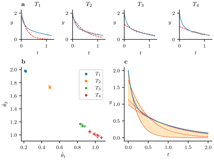
Figure 1: Under model discrepancy, parameter estimates from different training designs may vary significantly. (a): representative datasets generated by the data generating process shown with the solid blue line (Equation 1) with grey dots indicating observations (Equation 2). Panels from left to right use designs with observation times ($T_{1},T_{2},T_{3}\text{ and }T_{4}$). Here the fitted model (Equation 4, with optimized ${\boldsymbol{\theta}}$) is shown with the red dashed line. (b): a scatterplot of parameter estimates obtained from each protocol (using 10 repeats of the DGP). (c): a prediction made using the discrepant model trained using each of the protocols, for one repeat. Predictions obtained by training the models using different protocols are shown by the dashed lines, whereas the solid line shows the true DGP (Equation 1).

Then, we consider multiple experimental protocols which we may use to fit this model (Equation (4)). In particular, we consider four sets of observation times,

$$T_{1} =\left\{0,\,0.01,\,0.02,\,\ldots,0.01\right\},$$ (6)

$$T_{2} =\left\{0,\,0.1,\,0.2,\,0.3,\,\ldots,\,1\right\},$$ (7)

$$T_{3} =\left\{0.2,\,0.3,\,0.4,\,0.5,\,\ldots,\,1.2\right\},\;\text{ and }$$ (8)

$$T_{4} =\left\{0.5,\,0.55,\,0.6,\,\ldots,\,1\right\}.$$ (9)

For each $t\in T_{1},T_{2},T_{3},T_{4}$, we repeat the experiment 10 times by generating data from the DGP (Equation 2).

As shown in Fig. 1, training our discrepant model with each set of observation times yields four parameter estimates, each with different distributions. For instance, training using $T_{1}$ results in a model that approximates the DGP well on short timescales, and training using $T_{4}$ allows us to recapitulate the behaviour of the system over longer timescales, as can be seen in panel a. From how closely the model (Equation 4) fits the model in the regions where observations are made, we can see that in either of these cases, a single exponential seems to provide a reasonable approximation to the DGP. However, if we require an accurate model for both the slow and fast behaviour of the system, model discrepancy presents an issue, and this model may not be suitable.

1.2 Ion channel modelling

Discrepancy has proven to be a difficult problem to address in modelling electrically-excitable cells (electrophysiology modelling, Lei et al., 2020a; Mirams et al., 2016). The same is true for many other mathematical models, such as rainfall-runoff models in hydrology (Beven, 2006), models of the spread of infectious diseases in epidemiology (Guan et al., 2020; Creswell et al., 2023), and models used for the prediction of financial markets (Anderson et al., 2009).

The ‘rapid delayed rectifier potassium current’ (I_Kr), carried by the channel encoded primarily by hERG, plays an important role in the recovery of heart cells in from electrical stimulation. It allows the cell membrane to return to its ‘resting potential’ ahead of the next heartbeat. This current can be blocked by pharmaceutical drugs, disrupting this process and causing dangerous changes to heart rhythm. Mathematical models are now routinely used in drug safety assessment to test whether the expected dynamics of I_Kr under drug block are expected to cause such problems (Li et al., 2017). However, these models provide only an incomplete description of I_Kr, and do not, for example, account for the stochastic behaviour of individual ion channels (Mirams et al., 2016). For this reason, an understanding of model discrepancy and its implications is crucial in building accurate dynamical models of I_Kr, which permit a realistic appraisal of their predictive uncertainty.

In Section 1.1, we presented a simple example, in which each protocol corresponded to a particular choice of observation times. In electrophysiology voltage-clamp experiments, each protocol consists of a forcing function applied to the ODE system (the voltage applied to the cell over time as an input), together with a corresponding set of observation times for the resulting current (observed output). Electrophysiologists have a lot of control, and therefore choice, regarding the protocol design; but little work has been done to explore how the choice of protocol used to gather training data affects the accuracy of subsequent predictions. We explore these protocol-dependent effects of model discrepancy in Section 3.

1.3 Previously proposed methods to handle discrepancy

One way of reducing over-confidence in inaccurate parameter estimates in the presence of model discrepancy may be to use approximate Bayesian computation (ABC) (Frazier et al., 2020). With ABC, a likelihood function is not explicitly specified; instead, the model is repeatedly simulated for proposed values of the parameter sampled from a prior distribution. Each proposed value is accepted or rejected according to whether the simulated trajectory is “close” to the actual data, according to some summary statistics. Since ABC matches the simulated and real data by these summary statistics (rather than matching all aspects of the dynamics) and does so subject to a chosen tolerance — meaning that approximate matches are accepted — it is suited to inference where there is substantial model discrepancy, and decreases potential over-confidence in the inferred values of parameters. However, it is challenging to select suitable summary statistics, and the computational demands of ABC are much greater than those of the methods we propose.

Another approach was first introduced by Kennedy and O’Hagan (2001), who introduced Gaussian processes to the observables. This work has since been applied to electrophysiology models (Lei et al., 2020a). Elsewhere, Sung et al. introduced an approach to account for heteroscedastic errors using many repeats of the same experiment (Sung et al., 2020), although this seems to be less applicable to the hERG modelling problem (introduced in Section 2.2), as the number of repeats of each experiment (for cell-specific models) is limited. Alternatively, Lei and Mirams (2021) modelled the discrepancy using a neural network within the differential equations. However, these approaches reduce the interpretability of otherwise simple mechanistic models, and, when compared with models that simply ignore discrepancy, could potentially result in worse predictions under protocols that are dissimilar to those used for training.

Instead, we use a diverse range of experiments to train our models and build a picture of how model discrepancy manifests under different protocols. We are then able to judge the suitability of our models, and provide empirically-derived confidence intervals which provide a realistic level of predictive uncertainty due to model discrepancy. We demonstrate the utility of these methods under synthetically generated data by constructing two examples of model discrepancy.

2 Methods

We begin with a general overview of our proposed methods before providing two real-world examples of their applications. In Section 2.1.1, we outline some notation for a statistical model consisting of a dynamical system, an observation function, and some form of observational noise. This allows us to talk, in general terms, about model calibration and validation in Section 2.1.2. In particular, we describe a method for validating our models, in which we change the protocol used to train the model. This motivates our proposed methods for combining parameter estimates obtained from different protocols to empirically quantify model discrepancy for the prediction of unseen protocols.

2.1 Fitting models using multiple experimental protocols

2.1.1 Partially observable ODE models

In this paper, we restrict attention to deterministic models of biological phenomena, in which a system of ordinary differential equations (ODEs) is used to describe the deterministic time-evolution of some finite number of states, although the method would generalise to other types of models straightforwardly. This behaviour may be dependent on the protocol, $d$, chosen for the experiment, and so, we express our ODE system as,

$$\dfrac{\textrm{d}\mathbf{x}}{\textrm{d}t} =\mathbf{f}(\mathbf{x},t;{\boldsymbol{\theta}}_{f},d),$$ (10)

where $\mathbf{x}$ is a column vector of length $N$ describing the ‘state’ of the system, $t$ is time, and the parameters specifying the dynamics of the system are denoted ${\boldsymbol{\theta}}_{f}$. Additionally, the system is subject to some initial conditions which may be dependent on ${\boldsymbol{\theta}}$. Owing to $\mathbf{x}$’s dependence on the protocol and model parameters, we use the notation,

$$\mathbf{x}(t;{\boldsymbol{\theta}}_{f},d),$$ (11)

to denote the solution of Equation 10 under protocol $d$ and a specific choice of parameters, ${\boldsymbol{\theta}}_{f}$.

This ODE system is related to our noise-free observables via some observation function of the form,

$$h\left(\mathbf{x},t;{\boldsymbol{\theta}}_{h},d\right),$$ (12)

where $\mathbf{x}$ is the state of the ODE system (Equation 24), $t$ is the time that the observation occurs, $d$ is the protocol, and some additional parameters ${\boldsymbol{\theta}}_{h}$, which are distinct from those in ${\boldsymbol{\theta}}_{f}$. Here, we make observations of the system, via this function, at a set of observation times, $\{t_{i}\}_{i=1}^{n_{d}}$ defined by the protocol, $d$.

For concision, we may stack ${\boldsymbol{\theta}}_{f}$ and ${\boldsymbol{\theta}}_{h}$ into a single vector of model parameters,

$${\boldsymbol{\theta}}=\begin{bmatrix}{\boldsymbol{\theta}}_{f}\\ {\boldsymbol{\theta}}_{h}\end{bmatrix}.$$ (13)

Then, we denote an observation at time $t_{i}$ by

$$y_{i}({\boldsymbol{\theta}};d)=h\big{(}\mathbf{x}(t_{i};{\boldsymbol{\theta}}_{f},d),t_{i};{\boldsymbol{\theta}}_{h},d\big{)},$$ (14)

We denote the set of possible model parameters by $\Theta$, such that ${\boldsymbol{\theta}}\in\Theta$. We call this collection of possible parameter sets the parameter space.

For each protocol, $d\in\mathcal{D}$, and vector of model parameters, ${\boldsymbol{\theta}}$, we may combine each of our observations into a vector,

$$\mathbf{y}({\boldsymbol{\theta}};d)=\begin{bmatrix}y_{1}({\boldsymbol{\theta}};d),\\ \vdots\\ y_{n_{d}}({\boldsymbol{\theta}};d)\end{bmatrix}.$$ (15)

Additionally, we assume some form of random observational error such that, for each protocol, $d$, each observation is a random variable,

$$z_{i}(d)=y_{i}({\boldsymbol{\theta}};d)+\varepsilon_{i},$$ (16)

where each $\varepsilon_{i}$ is the error in the $i^{\text{th}}$ observation. Here each protocol, $d$, is performed exactly once so that we obtain one sample of each vector of observations ($\mathbf{z}(d)$). In the examples presented in Sections 3.1 and 3.2, we assume that our observations are subject to independent and identically distributed (IID) Gaussian errors, with mean, $0$, and standard deviation, $\sigma$.

2.1.2 Evaluation of predictive accuracy and model training

Given some parameter set ${\boldsymbol{\theta}}$, we may evaluate the accuracy of the resultant predictions under the application of some protocol $d\in\mathcal{D}$ by computing the root-mean-square-error (RMSE) between these predictions, and our observations ($\mathbf{z}(d)$),

$$\text{RMSE}\big{(}\mathbf{y}({\boldsymbol{\theta}};d),\;\mathbf{z}(d)\big{)}=\sqrt{\dfrac{1}{n_{d}}\sum_{i=1}^{n_{d}}\big{(}y_{i}({\boldsymbol{\theta}};d)-z_{i}(d)\big{)}^{2}},$$ (17)

where $n_{d}$ is the number of observations in protocol $d$. We choose the RMSE as it permits comparison between protocols with different numbers of observations.

Similarly, we may train our models to data, $\mathbf{z}(d)$, obtained using some protocol, $d$, by finding the parameter set that minimises this quantity (Equation 17). In this way, we define the parameter estimate obtained from protocol $d$ as,

$$\hat{\boldsymbol{\theta}}_{d}=\text{argmin}_{{\boldsymbol{\theta}}\in\Theta}\left\{\text{RMSE}\big{(}\mathbf{y}({\boldsymbol{\theta}},d),\;\mathbf{z}(d)\big{)}\right\},$$ (18)

which is a random variable. Since minimising the RMSE is equivalent to minimising the sum-of-square-errors, this estimate is also the least-squares estimator (identical to Equation 5). Moreover, under the assumption of Gaussian IID errors, Equation 18 is exactly the maximum likelihood estimator.

Having obtained such a parameter estimate, we may validate our model, by computing predictions for some other protocol, $\tilde{d}\in\mathcal{D}$. To do this, we compute, $\mathbf{y}(\hat{\boldsymbol{\theta}}_{d};\tilde{d}).$ This is a simulation of the behaviour of the system (without noise) under protocol $\tilde{d}$ made using parameter estimates that were obtained by training the model to protocol $d$ (as in Equation 18). In this way, our parameter estimates, each obtained from different protocols, result in, different out-of-sample predictions. Because we aim to train a model able to produce accurate predictions for all $d\in\mathcal{D}$, it is important to validate our model using multiple protocols.

By computing $\text{RMSE}\big{(}\mathbf{y}(\hat{\boldsymbol{\theta}}_{d};\tilde{d}),\mathbf{z}(\tilde{d})\big{)}$ for each pair of training and validation protocols, $d_{\text{train}},d_{\text{test}}$, we are able to perform model validation across multiple training and validation protocols. This allows us to ensure our models are robust with regard to the training protocol, and allow for the quantification of model discrepancy as demonstrated in Section 3.

2.1.3 Consequences of model error/discrepancy

Ideally, we would have a model that is correctly specified, in the sense that the data arise from the model being fitted. In other words, our observations $\mathbf{z}(d)$ arise from Equation 16 where ${\boldsymbol{\theta}}$ is some fixed, unknown value, ${\boldsymbol{\theta}}^{*}\in\Theta$. Then we may consider the distance between an estimate $\hat{\boldsymbol{\theta}}$ and the true value. Under suitable regularity conditions on the model and the design, $d$, when the fitted model is the true DGP, the estimator, $\hat{{\boldsymbol{\theta}}}(d)$, (Equation 18) is a ‘consistent’ estimator of the true parameter ${\boldsymbol{\theta}}^{*}$. This means that we can obtain arbitrarily accurate parameter estimates (where $\|\hat{\boldsymbol{\theta}}-{\boldsymbol{\theta}}^{*}\|$ is small) by collecting more data, that is, by increasing the number of observations. These regularity conditions include that, for the particular $d\in\mathcal{D}$, the model is structurally identifiable, meaning that different values of the parameter, ${\boldsymbol{\theta}}$, result in different model output (Wieland et al., 2021); and $\mathbf{y}({\boldsymbol{\theta}};d)$ is suitably smooth as a function of ${\boldsymbol{\theta}}$ (Seber and Wild, 2005).

However, when training discrepant models, we may find that our parameter estimates are heavily dependent on the training protocol, as demonstrated in Section 1.1. For unseen protocols, these discordant parameter sets may lead to a range of vastly different predictions, even if each parameter set provides a reasonable fit for its respective training protocol. In such a case, further data collection may reduce the variance of these parameter estimates, but fail to significantly improve the predictive accuracy of our models.

In Section 3, we explore two examples of synthetically constructed model discrepancy. In Section 3.1, we have that $\mathbf{f}$ and $h$ are exactly those functions used to generate the data, and the exact probability distribution of the observational errors is known, yet one parameter is fixed to an incorrect value. In other words, the true parameter set ${\boldsymbol{\theta}}^{*}$ lies outside the parameter space used in training the model. Under the assumption of structural identifiability (and a compact parameter space), this is an example of model discrepancy, because there is some limit to how well our model can recapitulate the DGP.

In Section 3.2 we explore another example of model discrepancy where our choice of $\mathbf{f}$ (and, in this case, the dimensions of ${\boldsymbol{\theta}}$ and $\mathbf{x}$) are misspecified by fitting a different model than the one used in the DGP.

2.1.4 Ensemble training and prediction interval

As outlined in Section 2.1.2, we can obtain parameter estimates from each protocol $d\in\mathcal{D}$ by finding the $\hat{\boldsymbol{\theta}}\in\Theta$ that minimises Equation 18. We then obtain an ensemble of parameter estimates,

$$\left\{\hat{\boldsymbol{\theta}}_{d}\;:\;d\in\mathcal{D}_{\text{train}}\right\}.$$ (19)

Then, for any validation protocol $\tilde{d}$, the set,

$$\left\{\mathbf{y}(\hat{\boldsymbol{\theta}}_{d};\tilde{d})\;:\;d\in\mathcal{D}_{\text{train}}\right\},$$

is an ensemble of predictions where $\mathcal{D}_{\text{train}}\subseteq\mathcal{D}$ is some set of training protocols. Each of these estimates may be used individually to make predictions. We may then use these ensembles of parameter estimates to attempt to quantify uncertainty in our prediction. We do this by considering the range of our predictions for each observation of interest. For the $i\text{th}$ observation of our validation protocol, $\tilde{d}$, that is

$$\mathcal{B}^{(i)} =\left[\mathcal{B}_{\text{lower}}^{(i)},\mathcal{B}_{\text{upper}}^{(i)}\right]$$ (20)

$$=\left[\min_{d\in\mathcal{D_{\text{train}}}}\left\{y_{i}(\hat{\boldsymbol{\theta}}(d);\tilde{d})\right\},\max_{d\in\mathcal{D_{\text{train}}}}\left\{y_{i}(\hat{\boldsymbol{\theta}}(d);\tilde{d})\right\}\right],$$ (21)

When all observations are considered at once, Equation 21 comprises a band of predictions, giving some indication of uncertainty in the predictions. We demonstrate below that this band provides a useful, empirical estimate of predictive error for unseen protocols, and provides a range of plausible predictions. For the purposes of a point estimate, we use the midpoint of each interval,

$$\mathcal{B}^{(i)}_{\text{mid}}=\dfrac{\mathcal{B}^{(i)}_{\text{lower}}+\mathcal{B}^{(i)}_{\text{upper}}}{2}.$$ (22)

This is used to assess the predictive error of the ensemble in Fig. 8. There are other ways to gauge the central tendency of the set of predictions (Equation 2.1.4). Such a change would have little effect on Section 3, but a median or weighted mean may be as (or more) suitable for other problems.

2.2 Application to an ion current model

We now turn our attention to an applied problem in which dynamical systems are used to model cellular electrophysiology. We apply our methods to two special cases of model discrepancy using synthetic data generation.

Firstly, we introduce a common paradigm for modelling macroscopic currents in electrically excitable cells, so-called Markov models (Rudy and Silva, 2006; Fink and Noble, 2009). In this setting, the term ‘Markov model’ is often used to refer to systems of ODEs where the state variables describe the proportional occupancy of some small collection of ‘states’, and the model parameters affect transition rates between these states. These models may be seen as a special case of the more general ODE model introduced in Section 2.1. Moreover, we briefly introduce some relevant electrophysiology and provide a detailed overview of our computational methods.

2.2.1 Markov models of I_Kr

Here, we use Markov models to describe the dynamics of I_Kr, especially in response to changes in the transmembrane potential. For any Markov model (as described above), the derivative function can be expressed in terms of a matrix, $\mathbf{A}$, which is dependent only on the voltage across the cell membrane, $V$. Accordingly, Equation 10 becomes,

$$\dfrac{\textrm{d}\mathbf{x}}{\textrm{d}t} =\mathbf{f}(\mathbf{x},t;{\boldsymbol{\theta}}_{f},d),$$ (23)

$$=\mathbf{A}\left(V(t;d);{\boldsymbol{\theta}}_{f}\right)\mathbf{x},$$ (24)

where $V(t;d)$ is the specified transmembrane potential at the time $t$ under protocol $d$. The elements of $\mathbf{A}(V;{\boldsymbol{\theta}}_{f})$, that is, $\mathbf{A}_{i,j}(V;{\boldsymbol{\theta}}_{f})$ describe the transition rate from state $j$ to state $i$ with transmembrane potential, $V$. Here $\mathbf{x}_{i}$ corresponds to the proportion of channels in some state. Usually, the transition rates (elements of $\mathbf{A}$) are either constant or of the form $\theta_{i}e^{\pm\theta_{j}V(t;d)}$ with $\theta_{i},\theta_{j}>0$.

Before and after each protocol, cells are left to equilibrate with the voltage $V$ set to the holding potential, $V_{\text{hold}}=-80$ mV. Therefore, we require the initial conditions, for at time $t=0$,

$$\mathbf{x}(0)=\mathbf{x}_{\infty}(V_{\text{hold}}),$$ (25)

where, $\mathbf{x}_{\infty}(V_{\text{hold}})$ is the unique steady-state solution for the linear system,

$$\dfrac{\textrm{d}\mathbf{x}}{\text{d}t}=\mathbf{A}(V_{\text{hold}};{\boldsymbol{\theta}}_{f})\mathbf{x},$$ (26)

subject to the constraint $\sum_{i=1}^{N}x_{i}(0)=1$. Note also that $\mathbf{A}(V_{\text{hold}};{\boldsymbol{\theta}}_{f})$ may be singular, as is the case when the number of channels is conserved ($\sum_{i=1}^{N}x_{i}(t)=1$ for all $t$). This is the case for both Markov models used in this paper. These models satisfy microscopic reversibility (Colquhoun et al., 2004), and so we may follow Fink and Noble’s method to find $\mathbf{x}_{\infty}$ (see Supplementary Material of Fink and Noble, 2009).

As is standard for models of I_Kr, we take our observation function to be

$$I_{\text{Kr}}=h(\mathbf{x},t_{i};\theta_{h},d)=g\cdot[O](t;{\boldsymbol{\theta}}_{f},d)\cdot(V(t;d)-E_{\text{Kr}}),$$ (27)

where $[O]$ denotes the proportion of channels in an ‘open’ conformation (one of the components of $\mathbf{x}$); and $g$ is the sole parameter in ${\boldsymbol{\theta}}_{h}$, known as the maximal conductance; and $E_{\text{Kr}}$ is the Nernst potential. $E_{\text{Kr}}$ is found by calculating

$$E_{\text{Kr}}=\dfrac{RT}{F}\ln\left\{\dfrac{[K_{\text{out}}]}{[K_{\text{in}}]}\right\},$$ (28)

where $R$ is the gas constant, $F$ is Faraday’s constant, and $T$ is the temperature and $[K_{\text{in}}]$ and $[K_{\text{out}}]$ are the intracellular and extracellular concentrations of $K^{+}$, respectively. Here, we choose the temperature to be room temperature ($T=293\text{K}$), and our intracellular and extracellular concentrations to be 120 mM and 5 mM, respectively. These are typical values which approximately correspond to physiological concentrations. Hence, for all synthetic data generation, training, and validation in Sections 3.1 and 3.2, we fix $E_{\text{Kr}}=-80.24~{}mV$ using Equation 28.

From Equations 24–27, we can see that both the dynamics of the model and the observation function are dependent on the voltage, $V(t;d)$. This is a special case of Equations 14–16, in which $\mathbf{f}$ and $h$ are time-dependent only via the voltage $V(t;d)$. In other words, at any fixed voltage ($V$), Equation 24 is an autonomous system and $h$ does not depend directly on $t$.

We assume that our observational errors are additive Gaussian IID random variables with zero mean and variance, $\sigma^{2}$.

The first model of I_Kr we consider is by Beattie et al. (2018). This is a four state Markov model with nine parameters (8 of which relate to the model’s kinetics and form ${\boldsymbol{\theta}}_{f}$). We use the parameters that Beattie et al. obtained from one particular cell (cell #5) by training their model to data obtained from an application of the ‘sinusoidal protocol’ with a manual patch-clamp setup. The cells used were Chinese hamster ovary cells, which were made to heterologously over-express hERG1a. These experiments were performed at room temperature.

The second model is by Wang et al. (1997). This is a five-state model which has $15$ parameters. These parameters were obtained by performing multiple voltage-clamp protocols, all at room temperature, on multiple frog oocytes overexpressing hERG. These experiments are used to infer activation and deactivation time constants as well as steady-state current voltage relations, which are, in turn, used to produce estimates for the model parameters. Of the two parameter sets provided in Wang et al. (1997), we use the parameter set obtained by using the extracellular solution with a 2 mM concentration of potassium chloride, as this most closely replicates physiological conditions.

The systems of ODEs for the Beattie and Wang models, as well as the parameterisations of the transition rates, are presented in Appendix A. The values of the model parameters, as used in Sections 3.1 and 3.2 are given in Table 1.

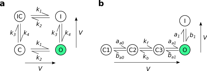
Figure 2: The structural differences between the two Markov model structures used in this paper for synthetic data generation and model training. (a): the four-state Beattie model used in both Case I and Case II. (b): the five-state Wang model used only for Case II. The open/conducting states are highlighted in green. The arrows adjacent to each model structure indicate the direction in which rates increase with more positive voltage.

2.2.2 Experimental Designs for Voltage Clamp Experiments

A large amount of data can be recorded in voltage-clamp electrophysiology experiments: the current is recorded at kHz samples for up to many minutes. In what follows, we take observations of the current at the same 10 kHz frequency for all protocols. Experimenters have a great deal of flexibility when it comes to specifying voltage-clamp protocol designs. We have published a number of studies on the benefits of ‘information-rich’ experimental designs for these protocols, focusing on short protocols which explore a wide range of voltages and timescales (Beattie et al., 2018; Lei et al., 2019a, b; Clerx et al., 2019a; Kemp et al., 2021). Here, we follow a similar theme using six short protocols, denoted $d_{0}$ to $d_{5}$, and shown in Fig. 3.

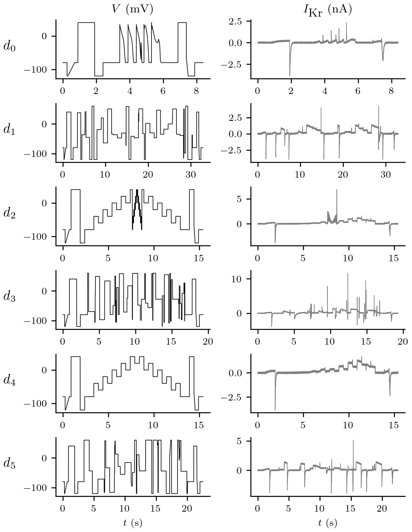
Figure 3: Left: a range of different input voltage-clamp protocols (forcing functions) used in this study. Right: corresponding synthetic output data I_Kr simulated using the Beattie model with noise added as described in Section 2.2.3. Here, we generate and plot data observed at a 10 kHz sampling rate. Training protocols (all protocols except $d_{0}$) were tested for numerical identifiability: inverse problems with different random noise forming their synthetic data yielded parameter estimates with little variability.

Here, we use simple designs consisting of a combination of sections where the voltage is held constant or ‘ramps’ where the voltage increases linearly with time for compatibility with automated high-throughput patch clamp machines which are restricted to protocols of this type. For the protocols included in this paper, short identical sequences including ramps are placed at the beginning and end of each protocol. In real experiments, these elements will allow for quality control, leak subtraction, and the estimation of the reversal potential (Lei et al., 2019a, b). The central portion, consisting of steps during which the voltage is held constant, is what varies between protocols.

Not all possible designs are suitable for training models. Sometimes we encounter protocols that result in very different parameter sets yielding approximately the same model output — i.e. the model output for a protocol is not sensitive to each parameter independently. Subsequently, when fitting the model to data generated from this protocol, many different parameter sets give an equally plausible fit. This problem is loosely termed numerical unidentifiability (Fink and Noble, 2009) and is generally best avoided for model training unless one can prove that future predictions in any protocol of interest will remain insensitive to the unidentified parameters.

For both the Beattie and Wang models, numerical unidentifiability is a problem for design $d_{0}$ (data not shown, but his phenomenon is illustrated for a similar I_Kr model and protocol in Fig. 3 of Whittaker et al. (2020)). Yet $d_{0}$ mimics the transmembrane voltage of a heart cell in a range of scenarios, and so provides a good way to validate whether our models recapitulate well-studied, physiologically-relevant behaviour. So in this study we use $d_{0}$ as a validation protocol, but do not use it as a training protocol for fitting models.

The remaining designs, $d_{1}$–$d_{5}$, were designed under various criteria with constraints on voltage ranges and step durations. $d_{1}$ was designed algorithmically by maximising the difference in model outputs between all pairs of global samples of parameters for the Beattie model; and $d_{5}$ was the result of the same algorithm applied to the Wang model. $d_{4}$ was manually designed, as a simplification of a sinusoidal approach we used previously, and presented in Lei et al. (2019a). $d_{2}$ is a further manual refinement of $d_{4}$ to explore inactivation processes (rapid loss of current at high voltages) more thoroughly. $d_{3}$ is based on maximising the exploration of the model phase-space for the Beattie model, visiting as many combinations of binned model states and voltages as possible. The main thing to note for this study however, is that $d_{1}$–$d_{5}$ result in good numerical identifiability for both models — that is, when used in synthetic data studies that attempt to re-infer the underlying parameters, all five protocol designs yield very low-variance parameter estimates (as shown in Fig. 5a for $\lambda=1$ for the Beattie model, and Fig. 7 for the Wang model). This is a useful property, because it allows us to disregard the (very small) effect of different random noise in the synthetic data on the spread of our predictions (Equation 21).

2.2.3 Computational Methods

Numerical solution of ODEs

Any time we calculate $\mathbf{y}({\boldsymbol{\theta}};d)$, we must solve a system of ordinary differential equations. We use a version of the LSODA solver designed to work with the Numba package, and Python to allow for the generation of efficient just-in-time compiled code from symbolic expressions. We partitioned each protocol into sections where the voltage is constant or changing linearly with respect to time because this sped up our computations. We set LSODA’s absolute and relative solver tolerances to $10^{-8}$. The fact that the total number of channels is conserved in our models, allows us to reduce the number of ODEs we need to solve from $N$ to $N-1$ (Fink and Noble, 2009).

Synthetic data generation

Having computed the state of the system at each observation time, $(\mathbf{x}(t_{i},{\boldsymbol{\theta}}^{*},d))_{i=1}^{n_{d}}$, it is simple to compute $y_{i}$ by substituting $\mathbf{x}$ into our observation function (Equation 16). Finally, to add noise, we obtain $n_{d}$ independent samples using Equation 16, using NumPy’s (Harris et al., 2020) interface to the PCG-64 pseudo-random number generator. Here, because we are using equally spaced observations with a 10 kHz sampling rate, $n_{d}=10,000\times t_{\text{duration}}$ where $t_{\text{duration}}$ is the length of the protocol’s voltage trace in seconds.

Optimisation

Finding the least-squares estimates, or, equivalently, minimising Equation 17 is (in general) a nonlinear optimisation problem for which there exist many numerical methods. We use CMA-ES (Hansen, 2006) as implemented by the PINTS interface (Clerx et al., 2019b). CMA-ES is a global, stochastic optimiser that has been applied successfully to many similar problems.

We follow the optimisation advice described in Clerx et al. (2019a). That is, for parameters ‘$a$’ and ‘$b$’ in state transition rates of the form $k=a\exp{(bV)}$, the optimiser works with ‘$\log a$’ and untransformed ‘$b$’ parameters. We enforce fairly lenient constraints on our parameter space, $\Theta$, to prevent a proposed parameter set from forcing transitions to become so fast/slow that the ODE system becomes very stiff and computationally difficult to solve. In particular, we require that every parameter is positive, and, for ease of computation,

$$10^{-9}\leq k(V)\leq 10^{7}$$ (29)

for all transition rates, $k$, for all $V\in[-120,\;40]$.

To ensure that we have found the global optimum, we repeat every optimisation numerous times using randomly sampled initial guesses. For each of these initial guesses, each kinetic parameter is sampled from,

$$\log_{10}(p)\sim U(-7,-1),$$ (30)

whereas we set the maximal conductance initial guess, which only affects the observation function, to the value used for data generation (even if these data were generated using a different model structure). We then check that our parameter set satisfies Equation 29, and resample if necessary before commencing the optimisation routine.

The examples presented in Sections 3.1 and 3.2 require the solution of many optimisation problems. For speed, these tasks may be organised in such a way that multiple optimisation problems can be solved in parallel.

3 Results

In this section, we use synthetically generated data to explore two cases of model discrepancy in Markov models of I_Kr. In this first case, we gradually introduce discrepancy into a model with the correct structure by fixing one of its parameters to values away from the DGP parameter set. Then, in Section 3.2, we apply the same methods to another case where the model structure is incorrectly specified. In both cases, we take a literature model of I_Kr together with Gaussian IID noise to be the DGP.

3.1 Case I: Misspecified maximal conductance

In this case, we assume a correctly specified model, but assume increasingly erroneous values of one particular parameter and investigate how this impacts the protocol-dependence of our parameter estimates and the predictive accuracy of our models. Also, we explore how the spread in our model predictions (Equation 21) increases as the amount of discrepancy increases (in some sense).

To do this, we fix the maximal conductance ($g$) to a range of values, and infer the remaining model parameters from synthetic data, generated using ${\boldsymbol{\theta}}^{*}$. Specifically, we take the true data generating process to be the Beattie model, as shown in Fig. 2. We simulate data generation from each training protocol, as outlined, ten times.

When training our models, we use a restriction of the usual parameter space to fit the data by assuming some fixed value, $\lambda$, for the maximal conductance, $g$. In this way, we reformulate the optimisation problem slightly such that Equation 18 becomes

$$\hat{\boldsymbol{\theta}}_{\lambda}(d)=\text{argmin}_{{\boldsymbol{\theta}}\in\Theta_{\lambda}}\left\{\text{RMSE}\left(\mathbf{y}({\boldsymbol{\theta}};d),\mathbf{z}(d)\right)\right\},$$ (31)

where $\Theta_{\lambda}$ is the subset of parameter space where the maximal conductance is fixed to $\lambda g$. For each repeat of each protocol, we solve this optimisation problem for each scaling factor, $\lambda\in\left\{\frac{1}{4},\frac{1}{2},1,2,4\right\}$. These calculations are almost identical to those used in the computation of profile likelihoods (Kreutz et al., 2013).

Next, we fit these restricted parameter-space models to the same dataset and assess their predictive power under the application of a validation protocol. We do this for each possible pair of training and validation protocols.

To reduce the time required for computation, for each repeat of each protocol, we fit our discrepant models sequentially. This is done so that, for example, the kinetic parameters found by fixing $\lambda=2$ are used as our initial guess when we fit the model with $\lambda=4$, unless the kinetic parameters (Table 1) provide a lesser RMSE than the results of the previous optimisation.

The spread in predictions for the validation protocol, $d_{0}$, for, $\lambda\in\{\frac{1}{4},1,4$} is shown in Fig. 4. A more complete summary of these results is provided by Fig. 5. Here, when $\lambda=1$ (the central row of Fig. 5), we can see that no matter what protocol is used to train the model, the distribution of parameter estimates seems to be centred around the true value of the parameters, and the resultant predictions all seem to be accurate. In contrast, when the maximal conductance, $g_{\text{Kr}}$ is set to an incorrect value, these predictions seem less accurate. Instead, our parameter estimates appear biased, and overall, our predictions become much less accurate. Moreover, the inaccuracy in our parameter estimates and our predictions varies depending on the design used to train the model. This effect does not appear to be symmetrical, with $\lambda<1$ seemingly resulting in more model discrepancy than $\lambda>1$.

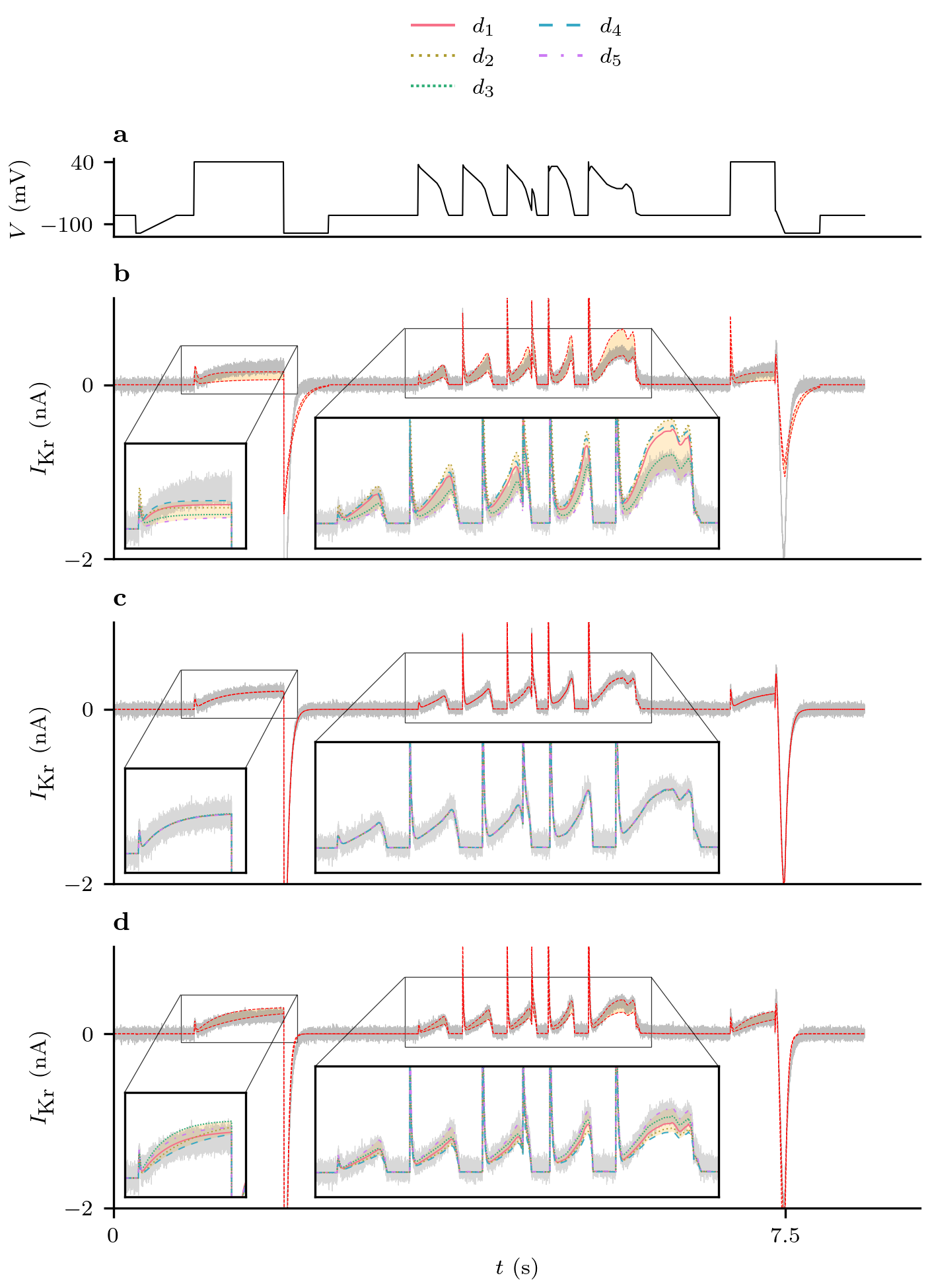
Figure 4: The set of predictions (Equation 2.1.4) shown for parameter estimates obtained by training to $d_{1},\ldots d_{5}$ (using the Beattie model) for different valu;es of $\lambda$. (a): the voltage trace for $d_{0}$. (b): The set of predictions with $\lambda=\frac{1}{4}$. (c): the set of predictions with $\lambda=1$, that is, under the assumption of the correct maximal conductance ($g$). (d): the set of predictions with $\lambda=4$ N.B. the ‘angular’ nature of the current is not a plotting artefact, but reflects the fact the voltage clamp (a) is constructed from a series of linear ramps for compatibility with automated voltage clamp machines.

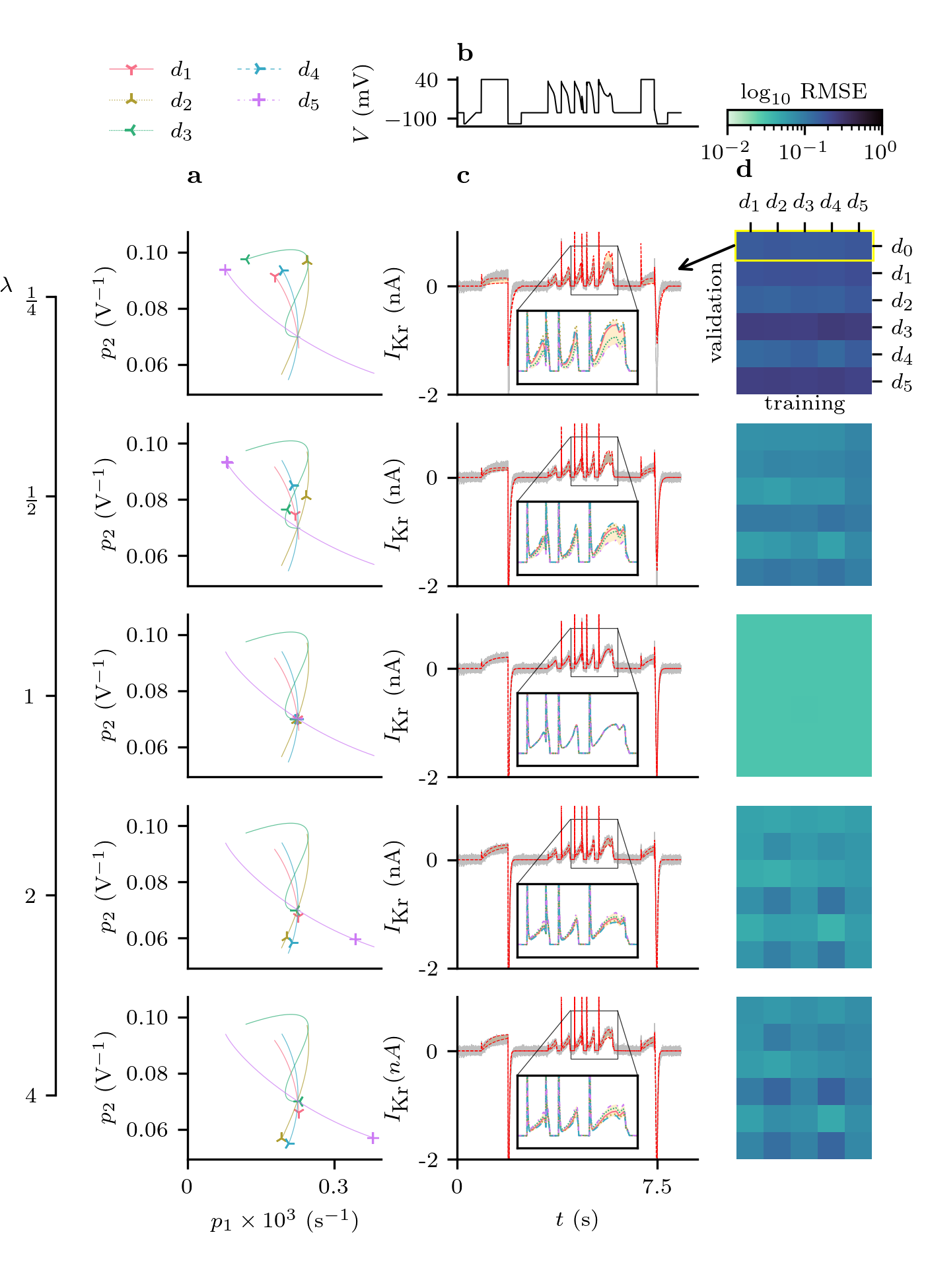
Figure 5: Discrepancy in parameter estimates and subsequent currents when a non-discrepant model is fitted to synthetic data, with all parameters free except the maximal conductance, g, which is fixed to $\lambda g^{*}$, where $g^{*}$ is the value used to generate the synthetic data. (a): estimates of $\theta_{1}$ and $\theta_{2}$ obtained by training with different protocols for 10 repeats of the DGP. A polynomial interpolation between these points is displayed as a visual aid. (b): $d_{0}$ voltage protocol. (c): the spread of predictions of $I_{\text{Kr}}$ under the $d_{0}$ protocol obtained from the parameter estimates in Column a. (d): a heatmap which summarises the predictive error obtained by training and validating using each pair of protocols. Note that Column c shows the top row of each heatmap, as indicated in the $\lambda=1/4$ case.

3.2 Case II: Misspecified dynamics

Next, we apply these methods to an example where we have misspecified the dynamics of the model (the function $\mathbf{f}$). We use two competing Markov models of hERG kinetics, the Beattie model (Beattie et al., 2018), and the Wang model (Wang et al., 1997). These models have differing structures and differing numbers of states, as shown in Fig. 2. We generate a synthetic dataset under the assumption of the Wang model with Gaussian IID noise and the original parameter set as given in Wang et al., for all the protocols shown in Fig. 3.

Then, we are able to fit both models to this dataset, obtaining an ensemble of parameter estimates and performing cross-validation as described in Section 2. In this way, we can assess the impact of choosing the wrong $\mathbf{f}$ in Equation 10, and its impact on the predictive accuracy of the model. We do this to investigate whether the techniques introduced in Section 2.1 are able to provide some useful quantification of model discrepancy when the dynamics of I_Kr are misspecified.

Our results, presented in Figs.  6 and 7, show how we expect a correctly specified model to behave in comparison to a discrepant model. We can see from the bottom row of Fig. 7, that when fitting using the correctly specified derivative matrix, we were able to accurately recover the true maximal conductance using each and every protocol. Moreover, similar to Case I, no matter which protocol the correctly specified model was trained with, the resultant predictions were very accurate.

However, we can see that when the discrepant model was used, there was significant protocol dependence in our parameter estimates, and our predictions were much less accurate overall, but perhaps accurate for many applications. Moreover, it seems that the for the majority of $d_{0}$, the spread in predictions across training protocols (Equation 21) was smaller than those seen in Case I. This may be due to the structural differences between the Wang and Beattie model. In particular, in the Wang model, channels transitioning from the high-voltage inactive state (I), must transition through the conducting, open state (O) in order to reach low-voltage closed states (C1, C2, C3), causing a spike of current to be observed. Instead, channels in the Beattie model may transition through the inactive-and-closed state (IC) on their way between O and C, resulting in reduced current during steps from high voltage to low voltage.

Nevertheless, our methods provide a useful indication of this model discrepancy. Fig. 8, examines the behaviour of our prediction interval (Equation 21) in more detail. Importantly, we can see that our interval shows little uncertainty during sections of the protocol where there is little current (and no reasonable model would predict any current). We can also see that our intervals show significant uncertainty around the spikes in current that occur at the start of each action-potential waveform. This is to be expected because it is known that these sections of the current time-series are particularly sensitive to differences in the rapid inactivation in these models (Clerx et al., 2019a).

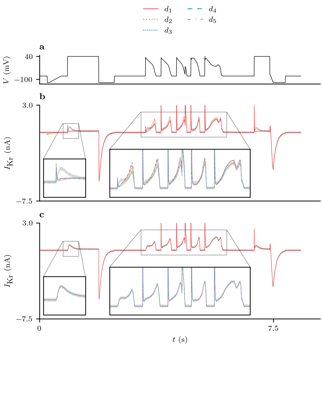
Figure 6: Case II: the set of predictions (Equation 2.1.4) shown for parameter estimates obtained by training to Wang data using the Beattie and Wang models. (a): the $d_{0}$ voltage-clamp protocol. (b): the set of predictions using the Beattie model. (c): the set of predictions with Wang model, that is, with under the assumption of the correct model structure.

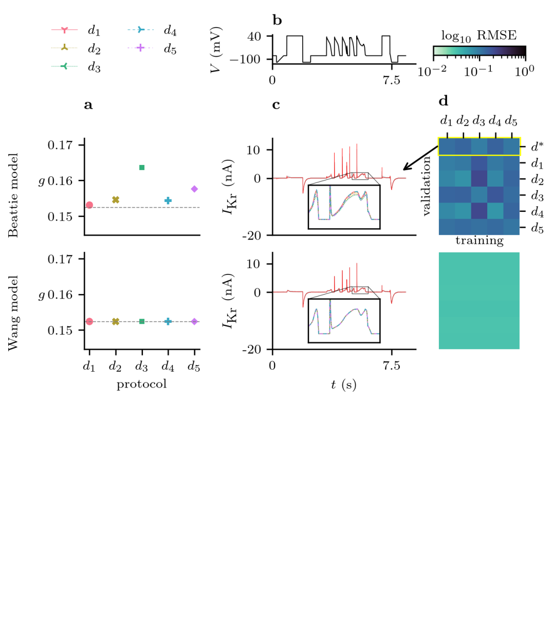
Figure 7: Model discrepancy between the Beattie model and data generated using the Wang model. (a): estimates of the maximal conductance obtained by fitting to different protocols for ten repeats of the DGP. There is a noticeable protocol dependence for estimates obtained using the (discrepant) Beattie model, but the true underlying parameter (dashed line) can be accurately determined from any protocol when using the (correct) Wang model. (b): $d_{0}$ voltage protocol. (c): the spread of predictions for $I_{\text{Kr}}$ under the $d_{0}$ protocol for discrepant (Beattie) and correct (Wang) models. (d): cross-validation heatmaps for both the Beattie and Wang models fitted to this suite of protocols, averaged over ten repeated samples of the DGP for each protocol.

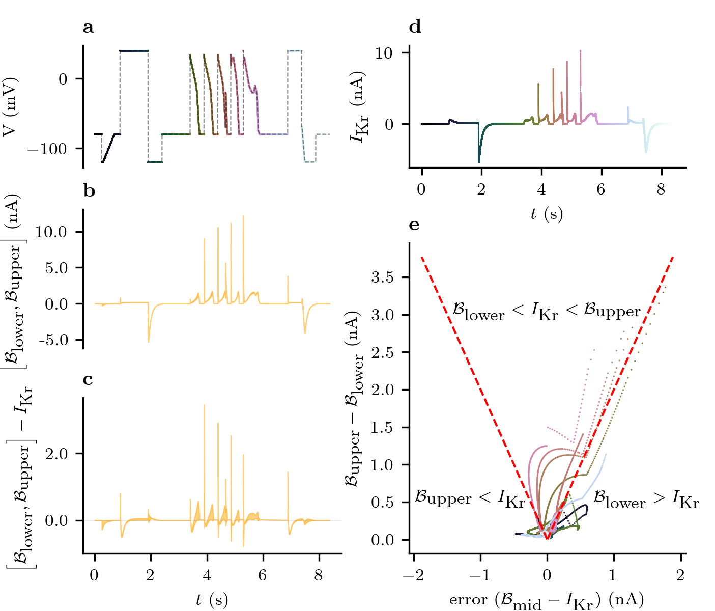
Figure 8: The spread in predictions obtained from different protocols provides a useful indicator of model discrepancy for Case II. (a): the validation voltage-clamp protocol, $d_{0}$, with colours corresponding to panels d and e. (b): the spread-of-predictions interval for $d_{0}$ using the Beattie model trained with $d_{1},\ldots,d_{5}$. (c): the true DGP subtracted from the spread-in-predictions interval. (d): the true DGP with the colour of each observation corresponding to panels a and e. (e): a scatter plot of the midpoint prediction (Equation 22) and the width of the predictive interval (Equation 21) for every observation in $d_{0}$. Here, the red, dashed lines show the true value of $I_{\text{Kr}}$ lies on the extremes of the range of predictions. Accordingly, points above these lines show the observations for which the DGP lies inside this range, and the points below the line correspond to observations for which the true DGP lies outside this range. The colours of these points correspond to those in panels a and d.

4 Discussion

We have introduced an uncertainty quantification (UQ) approach to highlight when discrepancy is affecting model predictions. We demonstrated the use of this technique by providing insight into the effects of model discrepancy on a model of I_Kr in electrically excitable cells. Here, we saw that under synthetically constructed examples of model discrepancy, there was great variability between the parameter estimates obtained using different experimental designs. This variability is a consequence of the different compromises that a discrepant model has to make to fit different regimes of a true DGP’s behaviour. Consequently, these parameter estimates produced a wide range of behaviour during validation.

The variability in the model predictions stemming from this ensemble of parameter estimates is, therefore, an empirical way of characterising the predictive uncertainty due to model discrepancy. Usefully, our spread-of-prediction intervals (Equation 21) correctly indicated little uncertainty when the ion channel model was exhibiting simple dynamics decaying towards a steady state, but more uncertainty during more complex dynamics, which was indeed when the largest discrepancies occurred. For many observations under our validation protocol, the true, underlying DGP lay inside this interval, indicating that Equation 21 may provide a useful indication of predictive error under unseen protocols. We expect that the methods presented may be of use for problems where the uncertainty in parameter estimates from one protocol is smaller than the variability between parameter estimates obtained from different protocols.

Figure 9: The Beattie and Wang models may be seen as special cases of this more complicated model. The state labelled ‘C/C3’ is called ‘C’ in the Beattie model and ‘C3’ in the Wang model. The arrows outside the Markov state diagram indicate the direction in which rates increase with more positive voltage.

The two examples of model discrepancy we presented are quite similar. The Beattie and Wang models can be regarded as two different special cases of a more general model shown in Fig. 9; these special cases arise with particular transition rate parameters in this larger model set to zero. Hence, there is a setting in which Case II is an example of the type of discrepancy explored in Case I, where a “true” parameter value exists in the more general model, but is excluded in the parameter space being optimised over for the model being fitted. This may prove a valuable perspective for modelling ion channel kinetics, where there are many candidate models (Mangold et al., 2021), and each model may be seen as corresponding to some subset of a general model with a shared higher-dimensional parameter space.

4.1 Limitations

Whilst the spread of predictions under some unseen protocol may provide some feasible range of predictions, we can see from Fig. 8, that the true DGP often lies outside this range. There is no guarantee that observations of the true DGP will lie inside or near our interval. As shown in Fig. 6, certain structural differences between the model and DGP may mean that the truth lies outside. For this reason, Equation 21 is best interpreted as a heuristic indication of predictive uncertainty stemming from model discrepancy, rather than providing any guarantees about the output of the DGP.

Using more training protocols in the training set may increase the coverage of the DGP by our interval. Whilst the number of protocols that can be performed on a single biological cell is limited by time constraints (Beattie et al., 2018; Lei et al., 2019b), the utilisation of more protocols is likely preferable.

Throughout Section 3, for our DGPs and models, we considered only additive Gaussian errors. But the differences we simulated between the underlying systems of deterministic ODEs describing the mechanistic model and assumed DGP are not the only possible source of model discrepancy: there can also be errors in the statistical/noise model. Or indeed, the DGP may not be accurately described by an ODE system, which we know to be the case when ion channel numbers are low and individual channels stochastically open and close. But our approach could also be employed for models involving stochastic differential equations (SDEs), as in Goldwyn et al. (2011), auto-correlated noise processes (e.g. as explored in Creswell et al., 2020; Lambert et al., 2022), or even experimental artefacts (Lei et al., 2020b), and it remains to be seen how well it would perform in these cases.

4.2 Future Directions

We were able to quantify model discrepancy by considering the predictive error of our models across a range of training and validation protocols. This provides a way of quantifying model discrepancy that can be compared across models, and could be used to select the most suitable model from a group of candidate models. By considering the spread of predictions across the entire design space, we may discard those models shown to produce the wider ranges of predictions. With such an approach, it would be trivial to identify the correctly specified models in Sections 3.1 and 3.2, for example.

Our approach may provide insight into improved experimental design criteria (Lei et al., 2022). Optimal experimental design approaches that assume knowledge of a correctly specified model may not be the most suitable in the presence of known discrepancy. By adjusting these approaches to account for the uncertainty in choice of model, we may be able to use these ideas to design experiments which allow for more robust model validation. One method would be to fit to data from a collection of training protocols, and to find a new protocol, for which the spread in ensemble predictions (Equation 21) is maximised.

The spread of predictions of our ensembles, based on training to data from multiple experimental designs, provides a good indication of possible predictive error due to model discrepancy. Ultimately, whilst our ensemble approach is no substitute for a correctly specified model, it is a useful tool for quantifying model discrepancy, predicting the size and direction of its effects, and may guide further experimental design and model selection approaches.

Data Availability

Open source code for all the simulation studies and plots in this paper can be found at https://github.com/CardiacModelling/empirical_quantification_of_model_discrepancy.

Appendix A A1: Parameterisation of Markov models

A.1 Beattie model

In full, the system of ODEs is,

$$\dfrac{\textrm{d}\mathbf{x}}{\text{d}t}=\left[\begin{matrix}-k_{1}-k_{3}&0&k_{4}&k_{2}\\ 0&-k_{2}-k_{4}&k_{1}&k_{3}\\ k_{3}&k_{2}&-k_{1}-k_{4}&0\\ k_{1}&k_{4}&0&-k_{2}-k_{3}\end{matrix}\right]\mathbf{x},$$ (32)

where

$$k_{1} =p_{1}e^{p_{2}V},$$ (33)

$$k_{2} =p_{3}e^{-Vp_{4}},$$ (34)

$$k_{3} =p_{5}e^{Vp_{6}}\hskip 10.00002pt,$$ (35)

$$k_{4} =p_{7}e^{-Vp_{8}}.$$ (36)

Hence, the corresponding parameter set is,

$${\boldsymbol{\theta}}=\begin{bmatrix}p_{1},\;\ldots,\;p_{8},\;g\end{bmatrix}^{T},$$ (37)

and,

$$\mathbf{x}=\begin{bmatrix}C,\;I,\;IC,\;O\end{bmatrix}^{T}.$$ (38)

A.2 Wang model

We may write this model’s governing system of ODEs as,

$$\dfrac{\textrm{d}\mathbf{x}}{\text{d}t}=\left[\begin{matrix}-a_{1}-b_{a_{1}}&0&0&a_{a_{1}}&b_{1}\\ 0&-a_{a0}&b_{a0}&0&0\\ 0&a_{a0}&-b_{a0}-k_{f}&k_{b}&0\\ b_{a1}&0&k_{f}&-a_{a1}-k_{b}&0\\ a_{1}&0&0&0&-b_{1}\end{matrix}\right]\mathbf{x}$$ (39)

where

$$a_{1} =q_{1}e^{Vq_{2}},$$ (40)

$$a_{a0} =q_{3}e^{Vq_{4}},$$ (41)

$$a_{a1} =q_{5}e^{Vq_{6}},$$ (42)

$$b_{a1} =q_{7}e^{-Vq_{8}},$$ (43)

$$b_{1} =q_{9}e^{-Vq_{10}},$$ (44)

$$b_{a0} =q_{11}e^{-Vq_{12}}.$$ (45)

The corresponding parameter set is,

$${\boldsymbol{\theta}}=\begin{bmatrix}q_{1},\;\ldots,\;q_{12},\;k_{f},\;k_{b}\end{bmatrix}^{T},$$ (47)

and

$$\mathbf{x}=\begin{bmatrix}O,\;C_{1},\;C_{2},\;C_{3},\;I\end{bmatrix}^{T}.$$ (48)

The default parameter values for both models are presented in Table 1.

Wang Model
Parameter	Value	Units
$q_{1}$	$2.23\times 10^{-2}$	ms-1
$q_{2}$	$1.18\times 10^{-2}$	mV-1
$q_{3}$	$4.70\times 10^{-2}$	ms-1
$q_{4}$	$6.31\times 10^{-2}$	mV-1
$q_{5}$	$1.37\times 10^{-2}$	ms-1
$q_{6}$	$3.82\times 10^{-3}$	mV-1
$q_{7}$	$6.89\times 10^{-5}$	ms-1
$q_{8}$	$3.16\times 10^{-2}$	mV-1
$q_{9}$	$4.18\times 10^{-2}$	mV-1
$q_{10}$	$9.08\times 10^{-2}$	mV-1
$q_{11}$	$2.34\times 10^{-2}$	mV-1
$q_{12}$	$6.50\times 10^{-3}$	mV-1
$k_{f}$	$2.38\times 10^{-2}$	mV-1
$k_{b}$	$3.68\times 10^{-2}$	mV-1
$g$	$1.52\times 10^{-1}$	$\mu$S

Beattie Model
Parameter	Value	Units
$p_{1}$	$2.26\times 10^{-4}$	ms-1
$p_{2}$	$6.99\times 10^{-2}$	mV-1
$p_{3}$	$3.45\times 10^{-5}$	ms-1
$p_{4}$	$5.46\times 10^{-2}$	mV-1
$p_{5}$	$8.73\times 10^{-2}$	ms-1
$p_{6}$	$8.91\times 10^{-3}$	mV-1
$p_{7}$	$5.15\times 10^{-3}$	ms-1
$p_{8}$	$3.16\times 10^{-2}$	mV-1
$g$	$1.52\times 10^{-1}$	$\mu$S

Table 1: The default parameter sets we use for the Wang et al. [1997] and Beattie et al. [2018] models. The same maximal conductance ($g$) is used for both models

References

- Smith [2013] Ralph C Smith. Uncertainty Quantification: theory, implementation, and applications, volume 12. Siam, 2013.
- Seber and Wild [2005] G.A.F. Seber and C.J. Wild. Nonlinear Regression. Wiley Series in Probability and Statistics. Wiley, 2005. ISBN 978-0-471-72530-5.
- Lei et al. [2020a] Chon Lok Lei, Sanmitra Ghosh, Dominic G. Whittaker, Yasser Aboelkassem, Kylie A. Beattie, Chris D. Cantwell, Tammo Delhaas, Charles Houston, Gustavo Montes Novaes, Alexander V. Panfilov, Pras Pathmanathan, Marina Riabiz, Rodrigo Weber dos Santos, John Walmsley, Keith Worden, Gary R. Mirams, and Richard D. Wilkinson. Considering discrepancy when calibrating a mechanistic electrophysiology model. Philosophical Transactions of the Royal Society A: Mathematical, Physical and Engineering Sciences, 378(2173):20190349, June 2020a. doi:10.1098/rsta.2019.0349.
- Mirams et al. [2016] Gary R Mirams, Pras Pathmanathan, Richard A Gray, Peter Challenor, and Richard H Clayton. Uncertainty and variability in computational and mathematical models of cardiac physiology. The Journal of Physiology, 594(23):6833–6847, 2016. doi:10.1113/JP271671.
- Beven [2006] Keith Beven. A manifesto for the equifinality thesis. Journal of Hydrology, 320(1):18–36, 2006. ISSN 0022-1694. doi:10.1016/j.jhydrol.2005.07.007.
- Guan et al. [2020] Jinxing Guan, Yongyue Wei, Yang Zhao, and Feng Chen. Modeling the transmission dynamics of COVID-19 epidemic: a systematic review. Journal of Biomedical Research, 34(6):422–430, November 2020. ISSN 1674-8301. doi:10.7555/JBR.34.20200119. URL https://www.ncbi.nlm.nih.gov/pmc/articles/PMC7718076/.
- Creswell et al. [2023] Richard Creswell, Martin Robinson, David Gavaghan, Kris V Parag, Chon Lok Lei, and Ben Lambert. A Bayesian nonparametric method for detecting rapid changes in disease transmission. Journal of Theoretical Biology, 558:111351, 2023. doi:10.1016/j.jtbi.2022.111351.
- Anderson et al. [2009] Evan W. Anderson, Eric Ghysels, and Jennifer L. Juergens. The impact of risk and uncertainty on expected returns. Journal of Financial Economics, 94(2):233–263, 2009. ISSN 0304-405X. doi:10.1016/j.jfineco.2008.11.001.
- Li et al. [2017] Zhihua Li, Sara Dutta, Jiansong Sheng, Phu N. Tran, Wendy Wu, Kelly Chang, Thembi Mdluli, David G. Strauss, and Thomas Colatsky. Improving the In Silico Assessment of Proarrhythmia Risk by Combining hERG (Human Ether-à-go-go-Related Gene) Channel–Drug Binding Kinetics and Multichannel Pharmacology. Circulation: Arrhythmia and Electrophysiology, 10(2):e004628, February 2017. doi:10.1161/CIRCEP.116.004628. URL https://www.ahajournals.org/doi/10.1161/CIRCEP.116.004628.
- Frazier et al. [2020] David T. Frazier, Christian P. Robert, and Judith Rousseau. Model misspecification in approximate bayesian computation: consequences and diagnostics. Journal of the Royal Statistical Society: Series B (Statistical Methodology), 82(2):421–444, 2020. doi:10.1111/rssb.12356.
- Kennedy and O’Hagan [2001] Marc C. Kennedy and Anthony O’Hagan. Bayesian calibration of computer models. Journal of the Royal Statistical Society: Series B (Statistical Methodology), 63(3):425–464, 2001. ISSN 1467-9868. doi:10.1111/1467-9868.00294. URL https://onlinelibrary.wiley.com/doi/abs/10.1111/1467-9868.00294.
- Sung et al. [2020] Chih-Li Sung, Beau David Barber, and Berkley J. Walker. Calibration of inexact computer models with heteroscedastic errors, May 2020. URL http://arxiv.org/abs/1910.11518.
- Lei and Mirams [2021] Chon Lok Lei and Gary R. Mirams. Neural network differential equations for ion channel modelling. Frontiers in Physiology, 12:1166, 2021. ISSN 1664-042X. doi:10.3389/fphys.2021.708944.
- Wieland et al. [2021] Franz-Georg Wieland, Adrian L. Hauber, Marcus Rosenblatt, Christian Tönsing, and Jens Timmer. On structural and practical identifiability. Current Opinion in Systems Biology, 25:60–69, 2021. ISSN 2452-3100. doi:10.1016/j.coisb.2021.03.005. URL https://www.sciencedirect.com/science/article/pii/S245231002100007X.
- Rudy and Silva [2006] Yoram Rudy and Jonathan R. Silva. Computational biology in the study of cardiac ion channels and cell electrophysiology. Quarterly reviews of biophysics, 39(1):57–116, February 2006. ISSN 0033-5835. doi:10.1017/S0033583506004227. URL https://www.ncbi.nlm.nih.gov/pmc/articles/PMC1994938/.
- Fink and Noble [2009] Martin Fink and Denis Noble. Markov models for ion channels: versatility versus identifiability and speed. Philosophical Transactions of the Royal Society A: Mathematical, Physical and Engineering Sciences, 367(1896):2161–2179, June 2009. doi:10.1098/rsta.2008.0301. URL https://royalsocietypublishing.org/doi/10.1098/rsta.2008.0301.
- Colquhoun et al. [2004] David Colquhoun, Kathryn A. Dowsland, Marco Beato, and Andrew J. R. Plested. How to Impose Microscopic Reversibility in Complex Reaction Mechanisms. Biophysical Journal, 86(6):3510–3518, June 2004. ISSN 0006-3495. doi:10.1529/biophysj.103.038679. URL https://www.ncbi.nlm.nih.gov/pmc/articles/PMC1304255/.
- Beattie et al. [2018] Kylie A. Beattie, Adam P. Hill, Rémi Bardenet, Yi Cui, Jamie I. Vandenberg, David J. Gavaghan, Teun P. de Boer, and Gary R. Mirams. Sinusoidal voltage protocols for rapid characterisation of ion channel kinetics. The Journal of Physiology, 596(10):1813–1828, 2018. ISSN 1469-7793. doi:10.1113/JP275733. URL https://physoc.onlinelibrary.wiley.com/doi/abs/10.1113/JP275733.
- Wang et al. [1997] S. Wang, S. Liu, M. J. Morales, H. C. Strauss, and R. L. Rasmusson. A quantitative analysis of the activation and inactivation kinetics of HERG expressed in Xenopus oocytes. The Journal of physiology, 502(1):45–60, July 1997. ISSN 0022-3751 1469-7793. doi:10.1111/j.1469-7793.1997.045bl.x.
- Lei et al. [2019a] Chon Lok Lei, Michael Clerx, Kylie A. Beattie, Dario Melgari, Jules C. Hancox, David J. Gavaghan, Liudmila Polonchuk, Ken Wang, and Gary R. Mirams. Rapid Characterization of hERG Channel Kinetics II: Temperature Dependence. Biophysical Journal, 117(12):2455–2470, December 2019a. ISSN 0006-3495. doi:10.1016/j.bpj.2019.07.030. URL https://www.sciencedirect.com/science/article/pii/S0006349519305983.
- Lei et al. [2019b] Chon Lok Lei, Michael Clerx, David J. Gavaghan, Liudmila Polonchuk, Gary R. Mirams, and Ken Wang. Rapid Characterization of hERG Channel Kinetics I: Using an Automated High-Throughput System. Biophysical Journal, 117(12):2438–2454, December 2019b. ISSN 0006-3495. doi:10.1016/j.bpj.2019.07.029. URL https://www.sciencedirect.com/science/article/pii/S0006349519305971.
- Clerx et al. [2019a] Michael Clerx, Kylie A. Beattie, David J. Gavaghan, and Gary R. Mirams. Four Ways to Fit an Ion Channel Model. Biophysical Journal, 117(12):2420–2437, December 2019a. ISSN 0006-3495. doi:10.1016/j.bpj.2019.08.001. URL http://www.sciencedirect.com/science/article/pii/S0006349519306666.
- Kemp et al. [2021] Jacob M. Kemp, Dominic G. Whittaker, Ravichandra Venkateshappa, ZhaoKai Pang, Raj Johal, Valentine Sergeev, Glen F. Tibbits, Gary R. Mirams, and Thomas W. Claydon. Electrophysiological characterization of the hERG R56Q LQTS variant and targeted rescue by the activator RPR260243. Journal of General Physiology, 153(10):e202112923, August 2021. ISSN 0022-1295. doi:10.1085/jgp.202112923. URL https://doi.org/10.1085/jgp.202112923.
- Whittaker et al. [2020] Dominic G. Whittaker, Michael Clerx, Chon Lok Lei, David J. Christini, and Gary R. Mirams. Calibration of ionic and cellular cardiac electrophysiology models. WIREs Systems Biology and Medicine, 12(4):e1482, 2020. ISSN 1939-005X. doi:10.1002/wsbm.1482. URL https://onlinelibrary.wiley.com/doi/abs/10.1002/wsbm.1482.
- Harris et al. [2020] Charles R Harris, K Jarrod Millman, Stéfan J Van Der Walt, Ralf Gommers, Pauli Virtanen, David Cournapeau, Eric Wieser, Julian Taylor, Sebastian Berg, Nathaniel J Smith, et al. Array programming with numpy. Nature, 585(7825):357–362, 2020. doi:10.1038/s41586-020-2649-2.
- Hansen [2006] Nikolaus Hansen. The CMA Evolution Strategy: a comparing review. In Jose A Lozano, Pedro Larrañaga, Iñaki Inza, and Endika Bengoetxea, editors, Towards a New Evolutionary Computation: Advances in the Estimation of Distribution Algorithms, pages 75–102. Springer-Verlag, Heidelberg, 2006. ISBN 978-3-540-32494-2. doi:10.1007/3-540-32494-1_4.
- Clerx et al. [2019b] Michael Clerx, Martin Robinson, Ben Lambert, Chon Lok Lei, Sanmitra Ghosh, Gary R Mirams, and David J Gavaghan. Probabilistic Inference on Noisy Time Series (PINTS). Journal of Open Research Software, 7(1):23, 2019b. doi:10.5334/jors.252.
- Kreutz et al. [2013] Clemens Kreutz, Andreas Raue, Daniel Kaschek, and Jens Timmer. Profile likelihood in systems biology. The FEBS Journal, 280(11):2564–2571, 2013. ISSN 1742-4658. doi:10.1111/febs.12276.
- Mangold et al. [2021] Kathryn E Mangold, Wei Wang, Eric K Johnson, Druv Bhagavan, Jonathan D Moreno, Jeanne M Nerbonne, and Jonathan R Silva. Identification of structures for ion channel kinetic models. PLoS Computational Biology, 17(8):e1008932, 2021. doi:10.1371/journal.pcbi.1008932.
- Goldwyn et al. [2011] Joshua H. Goldwyn, Nikita S. Imennov, Michael Famulare, and Eric Shea-Brown. Stochastic differential equation models for ion channel noise in Hodgkin-Huxley neurons. Phys. Rev. E, 83:041908, Apr 2011. doi:10.1103/PhysRevE.83.041908. URL https://link.aps.org/doi/10.1103/PhysRevE.83.041908.
- Creswell et al. [2020] Richard Creswell, Ben Lambert, Chon Lok Lei, Martin Robinson, and David Gavaghan. Using flexible noise models to avoid noise model misspecification in inference of differential equation time series models. arXiv preprint arXiv:2011.04854, 2020.
- Lambert et al. [2022] Ben Lambert, Chon Lok Lei, Martin Robinson, Michael Clerx, Richard Creswell, Sanmitra Ghosh, Simon Tavener, and David Gavaghan. Autocorrelated measurement processes and inference for ordinary differential equation models of biological systems. arXiv preprint arXiv:2210.01592, 2022. doi:10.48550/arXiv.2210.01592.
- Lei et al. [2020b] Chon Lok Lei, Michael Clerx, Dominic G. Whittaker, David J. Gavaghan, Teun P. de Boer, and Gary R. Mirams. Accounting for variability in ion current recordings using a mathematical model of artefacts in voltage-clamp experiments. Philosophical Transactions of the Royal Society A: Mathematical, Physical and Engineering Sciences, 378(2173):20190348, 2020b. doi:10.1098/rsta.2019.0348.
- Lei et al. [2022] Chon Lok Lei, Michael Clerx, David J Gavaghan, and Gary R Mirams. Model-driven optimal experimental design for calibrating cardiac electrophysiology models. bioRxiv, 2022. doi:10.1101/2022.11.01.514669.