On Over-Squashing in Message Passing Neural Networks:
The Impact of Width, Depth, and Topology

Abstract

Message Passing Neural Networks (MPNNs) are instances of Graph Neural Networks that leverage the graph to send messages over the edges. This inductive bias leads to a phenomenon known as over-squashing, where a node feature is insensitive to information contained at distant nodes. Despite recent methods introduced to mitigate this issue, an understanding of the causes for over-squashing and of possible solutions are lacking. In this theoretical work, we prove that: (i) Neural network width can mitigate over-squashing, but at the cost of making the whole network more sensitive; (ii) Conversely, depth cannot help mitigate over-squashing: increasing the number of layers leads to over-squashing being dominated by vanishing gradients; (iii) The graph topology plays the greatest role, since over-squashing occurs between nodes at high commute time. Our analysis provides a unified framework to study different recent methods introduced to cope with over-squashing and serves as a justification for a class of methods that fall under graph rewiring.

1 Introduction

Learning on graphs with Graph Neural Networks (GNNs) (Sperduti, 1993; Goller & Kuchler, 1996; Gori et al., 2005; Scarselli et al., 2008; Bruna et al., 2014; Defferrard et al., 2016) has become an increasingly flourishing area of machine learning. Typically, GNNs operate in the message-passing paradigm by exchanging information between nearby nodes (Gilmer et al., 2017), giving rise to the class of Message-Passing Neural Networks ($\mathsf{MPNN}$s). While message-passing has demonstrated to be a useful inductive bias, it has also been shown that the paradigm has some fundamental flaws, from expressivity (Xu et al., 2019; Morris et al., 2019), to over-smoothing (Nt & Maehara, 2019; Cai & Wang, 2020; Bodnar et al., 2022; Rusch et al., 2022; Di Giovanni et al., 2022b; Zhao et al., 2022) and over-squashing. The first two limitations have been thoroughly investigated, however less is known about over-squashing.

Alon & Yahav (2021) described over-squashing as an issue emerging when $\mathsf{MPNN}$s propagate messages across distant nodes, with the exponential expansion of the receptive field of a node leading to many messages being ‘squashed’ into fixed-size vectors. Topping et al. (2022) formally justified this phenomenon via a sensitivity analysis on the Jacobian of node features and, partly, linked it to the existence of edges with high-negative curvature. However, some important questions are left open from the analysis in Topping et al. (2022): (i) What is the impact of width in mitigating over-squashing? (ii) Can over-squashing be avoided by sufficiently deep models? (iii) How does over-squashing relate to the graph-spectrum and the underlying topology beyond curvature bounds that only apply to 2-hop propagation? The last point is particularly relevant due to recent works trying to combat over-squashing via methods that depend on the graph spectrum (Arnaiz-Rodríguez et al., 2022; Deac et al., 2022; Karhadkar et al., 2022). However, it is yet to be clarified if and why these works alleviate over-squashing.

In this work, we aim to address all the questions that are left open in Topping et al. (2022) to provide a better theoretical understanding on the causes of over-squashing as well as on what can and cannot fix it.

Contributions and outline.

An $\mathsf{MPNN}$ is generally constituted by two main parts: a choice of architecture, and an underlying graph over which it operates. In this work, we investigate how these factors participate in the over-squashing phenomenon. We focus on the width and depth of the $\mathsf{MPNN}$, as well as on the graph-topology.

• In Section 3, we prove that the width can mitigate over-squashing (Theorem 3.2), albeit at the potential cost of generalization. We also verify this with experiments.

• In Section 4, we show that depth may not be able to alleviate over-squashing. We identify two regimes. In the first one, the number of layers is comparable to the graph diameter, and we prove that over-squashing is likely to occur among distant nodes (Theorem 4.1). In fact, the distance at which over-squashing happens is strongly dependent on the graph topology – as we validate experimentally. In the second regime, we consider an arbitrary (large) number of layers. We prove that at this stage the $\mathsf{MPNN}$ is, generally, dominated by vanishing gradients (Theorem 4.2). This result is of independent interest, since it characterizes analytically conditions of vanishing gradients of the loss for a large class of $\mathsf{MPNN}$s that also include residual connections.

• In Section 5 we show that the topology of the graph has the greatest impact on over-squashing. In fact, we show that over-squashing happens among nodes with high commute time (Theorem 5.5) and we validate this empirically. This provides a unified framework to explain why all spatial and spectral rewiring approaches (discussed in Section 2.3) do mitigate over-squashing.

2 Background and related work

2.1 The message-passing paradigm

Let $\mathsf{G}$ be a graph with nodes $\mathsf{V}$ and edges $\mathsf{E}$. The connectivity is encoded in the adjacency matrix $\mathbf{A}\in\mathbb{R}^{n\times n}$, with $n$ the number of nodes. We assume that $\mathsf{G}$ is undirected, connected, and that there are features $\{\mathbf{h}_{v}^{(0)}\}_{v\in\mathsf{V}}\subset\mathbb{R}^{p}$. Graph Neural Networks (GNNs) are functions of the form $\mathsf{GNN}_{\theta}:(\mathsf{G},\{\mathbf{h}_{v}^{(0)}\})\mapsto y_{\mathsf{G}}$, with parameters $\theta$ estimated via training and whose output $y_{\mathsf{G}}$ is either a node-level or graph-level prediction. The most studied class of GNNs, known as the Message Passing Neural Network ($\mathsf{MPNN}$) (Gilmer et al., 2017), compute node representations by stacking $m$ layers of the form:

$$\mathbf{h}_{v}^{(t)}=\mathsf{com}^{(t)}(\mathbf{h}_{v}^{(t-1)},\mathsf{agg}^{(t)}(\{\mathbf{h}_{u}^{(t-1)}:(v,u)\in\mathsf{E}\})),$$

for $t=1,\ldots,m$, where $\mathsf{agg}^{(t)}$ is some aggregation function invariant to node permutation, while $\mathsf{com}^{(t)}$ combines the node’s current state with messages from its neighbours. In this work, we usually assume $\mathsf{agg}$ to be of the form

$$\mathsf{agg}^{(t)}(\{\mathbf{h}_{u}^{(t-1)}:(v,u)\in\mathsf{E}\})=\sum_{u}\boldsymbol{\mathsf{A}}_{vu}\mathbf{h}^{(t-1)}_{u},$$ (1)

where $\boldsymbol{\mathsf{A}}\in\mathbb{R}^{n\times n}$ is a Graph Shift Operator (GSO), meaning that $\boldsymbol{\mathsf{A}}_{vu}\neq 0$ if and only if $(v,u)\in\mathsf{E}$. Typically, $\boldsymbol{\mathsf{A}}$ is a (normalized) adjacency matrix that we also refer to as message-passing matrix. While instances of $\mathsf{MPNN}$ differ based on the choices of $\boldsymbol{\mathsf{A}}$ and $\mathsf{com}$, they all aggregate messages over the neighbours, such that in a layer, only nodes connected via an edge exchange messages. This presents two advantages: $\mathsf{MPNN}$s (i) can capture graph-induced ‘short-range’ dependencies well, and (ii) are efficient, since they can leverage the sparsity of the graph. Nonetheless, $\mathsf{MPNN}$s have been shown to suffer from a few drawbacks, including limited expressive power and over-squashing. The problem of expressive power stems from the equivalence of $\mathsf{MPNN}$s to the Weisfeiler-Leman graph isomorphism test (Xu et al., 2019; Morris et al., 2019). This framework has been studied extensively (Jegelka, 2022). On the other hand, the phenomenon of over-squashing, which is the main focus of this work, is more elusive and less understood. We review what is currently known about it in the next subsection.

2.2 The problem: introducing over-squashing

Since in an $\mathsf{MPNN}$ the information is aggregated over the neighbours, for a node $v$ to be affected by features at distance $r$, an $\mathsf{MPNN}$ needs at least $r$ layers (Barceló et al., 2019). It has been observed though that due to the expansion of the receptive field of a node, $\mathsf{MPNN}$s may end up sending a number of messages growing exponentially with the distance $r$, leading to a potential loss of information known as over-squashing (Alon & Yahav, 2021). Topping et al. (2022) showed that for an $\mathsf{MPNN}$ with message-passing matrix $\boldsymbol{\mathsf{A}}$ as in Eq. (1) and scalar features, given nodes $v,u$ at distance $r$, we have $\lvert\partial h_{v}^{(r)}/\partial h_{u}^{(0)}\rvert\leq c\cdot(\boldsymbol{\mathsf{A}}^{r})_{vu},$ with $c$ a constant depending on the Lipschitz regularity of the model. If $(\boldsymbol{\mathsf{A}}^{r})_{vu}$ decays exponentially with $r$, then the feature of $v$ is insensitive to the information contained at $u$. Moreover, Topping et al. (2022) showed that over-squashing is related to the existence of edges with high negative curvature. Such characterization though only applies to propagation of information up to 2 hops.

Figure 1: Effect of different rewirings $\mathcal{R}$ on the graph connectivity. The colouring denotes Commute Time – defined in Section 5 – w.r.t. to the star node. From left to right, the graphs shown are: the base, spatially rewired and spectrally rewired. The added edges significantly reduce the Commute Time and hence mitigate over-squashing in light of Theorem 5.5.

2.3 Related work

Multiple solutions to mitigate over-squashing have already been proposed. We classify them below; in Section 5, we provide a unified framework that encompasses all such solutions. We first introduce the following notion:

Definition 2.1.

Consider an $\mathsf{MPNN}$, a graph $\mathsf{G}$ with adjacency $\mathbf{A}$, and a map $\mathcal{R}:\mathbb{R}^{n\times n}\rightarrow\mathbb{R}^{n\times n}$. We say that $\mathsf{G}$ has been rewired by $\mathcal{R}$, if the messages are exchanged on $\mathcal{R}(\mathsf{G})$ instead of $\mathsf{G}$, with $\mathcal{R}(\mathsf{G})$ the graph with adjacency $\mathcal{R}(\mathbf{A})$.

Recent approaches to combat over-squashing share a common idea: replace the graph $\mathsf{G}$ with a rewired graph $\mathcal{R}(\mathsf{G})$ enjoying better connectivity Figure 1. We then distinguish these works based on the choice of the rewiring $\mathcal{R}$.

Spatial methods.

Since $\mathsf{MPNN}$s fail to propagate information to distant nodes, a solution consists in replacing $\mathsf{G}$ with $\mathcal{R}(\mathsf{G})$ such that $\mathrm{diam}(\mathcal{R}(\mathsf{G}))\ll\mathrm{diam}(\mathsf{G})$. Typically, this is achieved by either explicitly adding edges (possibly attributed) between distant nodes (Brüel-Gabrielsson et al., 2022; Abboud et al., 2022; Gutteridge et al., 2023) or by allowing distant nodes to communicate through higher-order structures (e.g., cellular or simplicial complexes, (Bodnar et al., 2021a, b), which requires additional domain knowledge and incurs a computational overhead). Graph-Transformers can be seen as an extreme example of rewiring, where $\mathcal{R}(\mathsf{G})$ is a complete graph with edges weighted via attention (Kreuzer et al., 2021; Mialon et al., 2021; Ying et al., 2021; Rampasek et al., 2022). While these methods do alleviate over-squashing, since they bring all pair of nodes closer, they come at the expense of making the graph $\mathcal{R}(\mathsf{G})$ much denser. In turn, this has an impact on computational complexity and introduces the risk of mixing local and non-local interactions.

We include in this group Topping et al. (2022) and Banerjee et al. (2022), where the rewiring is surgical – but requires specific pre-processing – in the sense that $\mathsf{G}$ is replaced by $\mathcal{R}(\mathsf{G})$ where edges have only been added to ‘mitigate’ bottlenecks as identified, for example, by negative curvature (Ollivier, 2007; Di Giovanni et al., 2022a).

We finally mention that spatial rewiring, intended as accessing information beyond the 1-hop when updating node features, is common to many existing frameworks (Abu-El-Haija et al., 2019; Klicpera et al., 2019; Chen et al., 2020; Ma et al., 2020; Wang et al., 2020; Nikolentzos et al., 2020). However, this is usually done via powers of the adjacency matrix, which is the main culprit for over-squashing (Topping et al., 2022). Accordingly, although the diffusion operators $\boldsymbol{\mathsf{A}}^{k}$ allow to aggregate information over non-local hops, they are not suited to mitigate over-squashing.

Spectral methods.

The connectedness of a graph $\mathsf{G}$ can be measured via a quantity known as the Cheeger constant, defined as follows (Chung & Graham, 1997):

Definition 2.2.

For a graph $\mathsf{G}$, the Cheeger constant is

$$\mathsf{h}_{\mathsf{Cheeg}}=\min_{\mathsf{U}\subset\mathsf{V}}\frac{\lvert\{(u,v)\in\mathsf{E}:u\in\mathsf{U},v\in\mathsf{V}\setminus\mathsf{U}\}\rvert}{\min(\mathrm{vol}(\mathsf{U}),\mathrm{vol}(\mathsf{V}\setminus\mathsf{U}))},$$

where $\mathrm{vol}(\mathsf{U})=\sum_{u\in\mathsf{U}}d_{u}$, with $d_{u}$ the degree of node $u$.

The Cheeger constant $\mathsf{h}_{\mathsf{Cheeg}}$ represents the energy required to disconnect $\mathsf{G}$ into two communities. A small $\mathsf{h}_{\mathsf{Cheeg}}$ means that $\mathsf{G}$ generally has two communities separated by only few edges – over-squashing is then expected to occur here if information needs to travel from one community to the other. While $\mathsf{h}_{\mathsf{Cheeg}}$ is generally intractable to compute, thanks to the Cheeger inequality we know that $\mathsf{h}_{\mathsf{Cheeg}}\sim\lambda_{1}$, where $\lambda_{1}$ is the positive, smallest eigenvalue of the graph Laplacian. Accordingly, a few new approaches have suggested to choose a rewiring that depends on the spectrum of $\mathsf{G}$ and yields a new graph satisfying $\mathsf{h}_{\mathsf{Cheeg}}(\mathcal{R}(\mathsf{G}))>\mathsf{h}_{\mathsf{Cheeg}}(\mathsf{G})$. This strategy includes Arnaiz-Rodríguez et al. (2022); Deac et al. (2022); Karhadkar et al. (2022). It is claimed that sending messages over such a graph $\mathcal{R}(\mathsf{G})$ alleviates over-squashing, however this has not been shown analytically yet.

The goal of this work.

The analysis of Topping et al. (2022), which represents our current theoretical understanding of the over-squashing problem, leaves some important open questions which we address in this work: (i) We study the role of the width in mitigating over-squashing; (ii) We analyse what happens when the depth exceeds the distance among two nodes of interest; (iii) We prove how over-squashing is related to the graph structure (beyond local curvature-bounds) and its spectrum. As a consequence of (iii), we provide a unified framework to explain how spatial and spectral approaches alleviate over-squashing. We reference here the concurrent work of Black et al. (2023), who, similarly to us, drew a strong connection between over-squashing and Effective Resistance (see Section 5).

Notations and conventions to improve readability.

In the following, to prioritize readability we often leave sharper bounds with more optimal and explicit terms to the Appendix. From now on, $p$ always denotes the width (hidden dimension) while $m$ is the depth (i.e. number of layers). The feature of node $v$ at layer $t$ is written as $\mathbf{h}_{v}^{(t)}$. Finally, we write $[\ell]=\{1,\ldots,\ell\}$ for any integer $\ell$. All proofs can be found in the Appendix.

3 The impact of width

In this Section we assess whether the width of the underlying $\mathsf{MPNN}$ can mitigate over-squashing and the extent to which this is possible. In order to do that, we extend the sensitivity analysis in Topping et al. (2022) to higher-dimensional node features. We consider a class of $\mathsf{MPNN}$s parameterised by neural networks, of the form:

$$\mathbf{h}_{v}^{(t+1)}=\sigma\Big{(}c_{\mathsf{r}}\mathbf{W}_{\mathsf{r}}^{(t)}\mathbf{h}_{v}^{(t)}+c_{\mathsf{a}}\mathbf{W}_{\mathsf{a}}^{(t)}\sum_{u}\boldsymbol{\mathsf{A}}_{vu}\mathbf{h}^{(t)}_{u}\Big{)},$$ (2)

where $\sigma$ is a pointwise-nonlinearity, $\mathbf{W}_{\mathsf{r}}^{(t)},\mathbf{W}_{\mathsf{a}}^{(t)}\in\mathbb{R}^{p\times p}$ are learnable weight matrices and $\boldsymbol{\mathsf{A}}$ is a graph shift operator. Note that Eq. (2) includes common $\mathsf{MPNN}$s such as $\mathsf{GCN}$ (Kipf & Welling, 2017), $\mathsf{SAGE}$ (Hamilton et al., 2017), and $\mathsf{GIN}$ (Xu et al., 2019), where $\boldsymbol{\mathsf{A}}$ is one of $\mathbf{D}^{-1/2}\mathbf{A}\mathbf{D}^{-1/2}$, $\mathbf{D}^{-1}\mathbf{A}$ and $\mathbf{A}$, respectively, with $\mathbf{D}$ the diagonal degree matrix. In Appendix B, we extend the analysis to a more general class of $\mathsf{MPNN}$s (see Theorem B.1), which includes stacking multiple nonlinearities. We also emphasize that the positive scalars $c_{\mathsf{r}},c_{\mathsf{a}}$ represent the weighted contribution of the residual term and of the aggregation term, respectively. To ease the notations, we introduce a family of message-passing matrices that depend on $c_{\mathsf{r}},c_{\mathsf{a}}$.

Definition 3.1.

For a graph shift operator $\boldsymbol{\mathsf{A}}$ and constants $c_{\mathsf{r}},c_{\mathsf{a}}>0$, we define $\boldsymbol{\mathsf{S}}_{\mathsf{r},\mathsf{a}}:=c_{\mathsf{r}}\mathbf{I}+c_{\mathsf{a}}\boldsymbol{\mathsf{A}}\in\mathbb{R}^{n\times n}$ to be the message-passing matrix adopted by the $\mathsf{MPNN}$.

As in Xu et al. (2018) and Topping et al. (2022), we study the propagation of information in the $\mathsf{MPNN}$ via the Jacobian of node features after $m$ layers.

Theorem 3.2 (Sensitivity bounds).

Consider an $\mathsf{MPNN}$ as in Eq. (2) for $m$ layers, with $c_{\sigma}$ the Lipschitz constant of the nonlinearity $\sigma$ and $w$ the maximal entry-value over all weight matrices. For $v,u\in\mathsf{V}$ and width $p$, we have

$$\left\|\frac{\partial\mathbf{h}_{v}^{(m)}}{\partial\mathbf{h}_{u}^{(0)}}\right\|_{L_{1}}\leq(\underbrace{\vphantom{\boldsymbol{\mathsf{S}}_{\mathsf{r},\mathsf{a}}^{m}}c_{\sigma}wp}_{\mathrm{model}})^{m}\underbrace{(\boldsymbol{\mathsf{S}}_{\mathsf{r},\mathsf{a}}^{m})_{vu}}_{\mathrm{topology}},$$ (3)

with $\boldsymbol{\mathsf{S}}_{\mathsf{r},\mathsf{a}}^{m}$ the $m^{th}$-power of $\boldsymbol{\mathsf{S}}_{\mathsf{r},\mathsf{a}}$ introduced in Definition 3.1.

Over-squashing occurs if the right hand side of Eq. (3) is too small – this will be related to the distance among $v$ and $u$ in Section 4.1. A small derivative of $\mathbf{h}_{v}^{(m)}$ with respect to $\mathbf{h}_{u}^{(0)}$ means that after $m$ layers, the feature at $v$ is mostly insensitive to the information initially contained at $u$, and hence that messages have not been propagated effectively. Theorem 3.2 clarifies how the model can impact over-squashing through (i) its Lipschitz regularity $c_{\sigma},w$ and (ii) its width $p$. In fact, given a graph $\mathsf{G}$ such that $(\boldsymbol{\mathsf{S}}_{\mathsf{r},\mathsf{a}}^{m})_{vu}$ decays exponentially with $m$, the $\mathsf{MPNN}$ can compensate by increasing the width $p$ and the magnitude of $w$ and $c_{\sigma}$. This confirms analytically the discussion in Alon & Yahav (2021): a larger hidden dimension $p$ does mitigate over-squashing. However, this is not an optimal solution since increasing the contribution of the model (i.e. the term $c_{\sigma}wp$) may lead to over-fitting and poorer generalization (Bartlett et al., 2017). Taking larger values of $c_{\sigma},w,p$ affects the model globally and does not target the sensitivity of specific node pairs induced by the topology via $\boldsymbol{\mathsf{S}}_{\mathsf{r},\mathsf{a}}$.

Validating the theoretical results.

We validate empirically the message from Theorem 3.2: if the task presents long-range dependencies, increasing the hidden dimension mitigates over-squashing and therefore has a positive impact on the performance. We consider the following ‘graph transfer’ task, building upon Bodnar et al. (2021a): given a graph, consider source and target nodes, placed at distance $r$ from each other. We assign a one-hot encoded label to the target and a constant unitary feature vector to all other nodes. The goal is to assign to the source node the feature vector of the target. Partly due to over-squashing, performance is expected to degrade as $r$ increases.

To validate that this holds irrespective of the graph structure, we evaluate across three graph topologies, called $\mathsf{CrossedRing}$, $\mathsf{Ring}$ and $\mathsf{CliquePath}$ - see Appendix E for further details. While the topology is also expected to affect the performance (as confirmed in Section 4), given a fixed topology, we expect the model to benefit from an increase of hidden dimension.

To verify this behaviour, we evaluate $\mathsf{GCN}$ (Kipf & Welling, 2017) on the three graph transfer tasks increasing the hidden dimension, but keeping the number of layers equal to the distance between source and target, as shown in Figure 2. The results verify the intuition from the theorem that a higher hidden dimension helps the $\mathsf{GCN}$ model solve the task to larger distances across the three graph-topologies.

Figure 2: Performance of $\mathsf{GCN}$ on the $\mathsf{CrossedRing}$, $\mathsf{Ring}$, and $\mathsf{CliquePath}$ tasks obtained by varying the hidden dimension. Increasing the hidden dimension helps mitigate the over-squashing effect, in accordance with Theorem 3.2.

4 The impact of depth

Consider a graph $\mathsf{G}$ and a task with ‘long-range’ dependencies, meaning that there exists (at least) a node $v$ whose embedding has to account for information contained at some node $u$ at distance $r\gg 1$. One natural attempt at resolving over-squashing amounts to increasing the number of layers $m$ to compensate for the distance. We prove that the depth of the $\mathsf{MPNN}$ will, generally, not help with over-squashing. We show that: (i) When the depth $m$ is comparable to the distance, over-squashing is bound to occur among distant nodes – in fact, the distance at which over-squashing happens, is strongly dependent on the underlying topology; (ii) If we take a large number of layers to cover the long-range interactions, we rigorously prove under which exact conditions, $\mathsf{MPNN}$s incur the vanishing gradients problem.

4.1 The shallow-diameter regime: over-squashing occurs among distant nodes

Consider the scenario above, with two nodes $v,u$, whose interaction is important for the task, at distance $r$. We first focus on the regime $m\sim r$. We refer to this as the shallow-diameter regime, since the number of layers $m$ is comparable to the diameter of the graph.

From now on, we set $\boldsymbol{\mathsf{A}}=\mathbf{D}^{-1/2}\mathbf{A}\mathbf{D}^{-1/2}$, where we recall that $\mathbf{A}$ is the adjacency matrix and $\mathbf{D}$ is the degree matrix. This is not restrictive, but allows us to derive more explicit bounds and, later, bring into the equation the spectrum of the graph. We note that results can be extended easily to $\mathbf{D}^{-1}\mathbf{A}$, given that this matrix is similar to $\boldsymbol{\mathsf{A}}$, and, in expectation, to $\mathbf{A}$ by normalizing the Jacobian as in Xu et al. (2019) and Section A in the Appendix of Topping et al. (2022).

Theorem 4.1 (Over-squashing among distant nodes).

Given an $\mathsf{MPNN}$ as in Eq. (2), with $c_{\mathsf{a}}\leq 1$, let $v,u\in\mathsf{V}$ be at distance $r$. Let $c_{\sigma}$ be the Lipschitz constant of $\sigma$, $w$ the maximal entry-value over all weight matrices, $d_{\mathrm{min}}$ the minimal degree of $\mathsf{G}$, and $\gamma_{\ell}(v,u)$ the number of walks from $v$ to $u$ of maximal length $\ell$. For any $0\leq k<r$, there exists $C_{k}>0$ independent of $r$ and of the graph, such that

$$\left\|\frac{\partial\mathbf{h}_{v}^{(r+k)}}{\partial\mathbf{h}_{u}^{(0)}}\right\|_{L_{1}}\leq C_{k}\gamma_{r+k}(v,u)\Big{(}\frac{2c_{\sigma}wp}{d_{\mathrm{min}}}\Big{)}^{r}.$$ (4)

To understand the bound above, fix $k<r$ and assume that nodes $v,u$ are ‘badly’ connected, meaning that the number of walks $\gamma_{r+k}(v,u)$ of length at most $r+k$, is small. If $2\,c_{\sigma}wp<d_{\mathrm{min}}$, then the bound on the Jacobian in Eq. (4) decays exponentially with the distance $r$. Note that the bound above considers $d_{\mathrm{min}}$ and $\gamma_{r+k}$ as a worst case scenario. If one has a better understanding of the topology of the graph, sharper bounds can be derived by estimating $(\boldsymbol{\mathsf{S}}_{\mathsf{r},\mathsf{a}}^{r})_{vu}$. Theorem 4.1 implies that, when the depth $m$ is comparable to the diameter of $\mathsf{G}$, over-squashing becomes an issue if the task depends on the interaction of nodes $v,u$ at ‘large’ distance $r$. In fact, Theorem 4.1 shows that the distance at which the Jacobian sensitivity falls below a given threshold, depends on both the model, via $c_{\sigma},w,p$, and on the graph, through $d_{\mathrm{min}}$ and $\gamma_{r+k}(v,u)$. We finally observe that Theorem 4.1 generalizes the analysis in Topping et al. (2022) in multiple ways: (i) it holds for any width $p>1$; (ii) it includes cases where $m>r$; (iii) it provides explicit estimates in terms of number of walks and degree information.

Remark. What if $2c_{\sigma}wp>d_{\mathrm{min}}$? Taking larger weights and hidden dimension increases the sensitivity of node features. However, this occurs everywhere in the graph the same. Accordingly, nodes at shorter distances will, on average, still have sensitivity exponentially larger than nodes at large distance. This is validated in our synthetic experiments below, where we do not have constraints on the weights.

Validating the theoretical results.

From Theorem 4.1, we derive a strong indication of the difficulty of a task by calculating an upper bound on the Jacobian. We consider the same graph transfer tasks introduced above, namely $\mathsf{CrossedRing}$, $\mathsf{Ring}$, and $\mathsf{CliquePath}$. For these special cases, we can derive a refined version of the r.h.s in Eq. (4): in particular, $k=0$ (i.e. the depth coincides with the distance among source and target) and the term $\gamma_{r}(v,u)(d_{\mathrm{min}})^{-r}$ can be replaced by the exact quantity $(\boldsymbol{\mathsf{S}}_{\mathsf{r},\mathsf{a}}^{r})_{vu}$. Fixing a distance $r$ between source $u$ and target $v$ then, if we consider for example the $\mathsf{GCN}$-case, we have $\boldsymbol{\mathsf{S}}_{\mathsf{r},\mathsf{a}}=\boldsymbol{\mathsf{A}}$ so that the term $(\boldsymbol{\mathsf{S}}_{\mathsf{r},\mathsf{a}}^{r})_{vu}$ can be computed explicitly:

$$(\boldsymbol{\mathsf{S}}_{\mathsf{r},\mathsf{a}}^{r})_{vu}=(3/2)^{-(r-1)}\qquad \text{ for }\mathsf{CrossedRing}$$

$$(\boldsymbol{\mathsf{S}}_{\mathsf{r},\mathsf{a}}^{r})_{vu}=2^{-(r-1)}\quad \text{ for }\mathsf{Ring}$$

$$(\boldsymbol{\mathsf{S}}_{\mathsf{r},\mathsf{a}}^{r})_{vu}=2^{-(r-2)}/(r\sqrt{r-2}) \text{ for }\mathsf{CliquePath}.$$

Given an $\mathsf{MPNN}$, terms like $c_{\sigma},w,p$ entering Theorem 4.1 are independent of the graph-topology and hence can be assumed to behave, roughly, the same across different graphs. As a consequence, we can expect over-squashing to be more problematic for $\mathsf{CliquePath}$, followed by $\mathsf{Ring}$, and less prevalent comparatively in $\mathsf{CrossedRing}$. Figure 3 shows the behaviour of $\mathsf{GIN}$ (Xu et al., 2019), $\mathsf{SAGE}$ (Hamilton et al., 2017), $\mathsf{GCN}$ (Kipf & Welling, 2017), and $\mathsf{GAT}$ (Veličković et al., 2018) on the aformentioned tasks. We verify the conjectured difficulty. $\mathsf{CliquePath}$ is the consistently hardest task, followed by $\mathsf{Ring}$, and $\mathsf{CrossedRing}$. Furthermore, the decay of the performance to random guessing for the same architecture across different graph topologies highlights that this drop cannot be simply labelled as ‘vanishing gradients’ since for certain topologies the same model can, in fact, achieve perfect accuracy. This validates that the underlying topology has a strong impact on the distance at which over-squashing is expected to happen. Moreover, we confirm that in the regime where the depth $m$ is comparable to the distance $r$, over-squashing will occur if $r$ is large enough.

Figure 3: Performance of $\mathsf{GIN}$, $\mathsf{SAGE}$, $\mathsf{GCN}$, and $\mathsf{GAT}$ on the $\mathsf{CliquePath}$, $\mathsf{Ring}$, and $\mathsf{CrossedRing}$ tasks. In the case where depth and distance are comparable, over-squashing highly depends on the topology of the graph as we increase the distance.

4.2 The deep regime: vanishing gradients dominate

We now focus on the regime where the number of layers $m\gg r$ is large. We show that in this case, vanishing gradients can occur and make the entire model insensitive. Given a weight $\theta^{(k)}$ entering a layer $k$, one can write the gradient of the loss after $m$ layers as (Pascanu et al., 2013)

$$\frac{\partial\mathcal{L}}{\partial\theta^{(k)}}=\sum_{v,u\in V}\Big{(}\frac{\partial\mathcal{L}}{\partial\mathbf{h}^{(m)}_{v}}\frac{\partial\mathbf{h}_{u}^{(k)}}{\partial\vphantom{\mathbf{h}^{(k)}_{u}}\theta^{(k)}}\Big{)}\underbrace{\frac{\partial\mathbf{h}_{v}^{(m)}}{\partial\mathbf{h}_{u}^{(k)}}}_{\mathrm{sensitivity}}$$ (5)

We provide exact conditions for $\mathsf{MPNN}$s to incur the vanishing gradient problem, intended as the gradients of the loss decaying exponentially with the number of layers $m$.

Theorem 4.2 (Vanishing gradients).

Consider an $\mathsf{MPNN}$ as in Eq. (2) for $m$ layers with a quadratic loss $\mathcal{L}$. Assume that (i) $\sigma$ has Lipschitz constant $c_{\sigma}$ and $\sigma(0)=0$, and (ii) weight matrices have spectral norm bounded by $\mu>0$. Given any weight $\theta$ entering a layer $k$, there exists a constant $C>0$ independent of $m$, such that

$$\left|\frac{\partial\mathcal{L}}{\partial\theta}\right| \leq C\left(c_{\sigma}\mu(c_{\mathsf{r}}+c_{\mathsf{a}})\right)^{m-k}\left(1+\left(c_{\sigma}\mu(c_{\mathsf{r}}+c_{\mathsf{a}})\right)^{m}\right).$$ (6)

In particular, if $c_{\sigma}\mu(c_{\mathsf{r}}+c_{\mathsf{a}})<1$, then the gradients of the loss decay to zero exponentially fast with $m$.

The problem of vanishing gradients for graph convolutional networks have been studied from an empirical perspective (Li et al., 2019, 2021). Theorem 4.2 provides sufficient conditions for the vanishing of gradients to occur in a large class of $\mathsf{MPNN}$s that also include (a form of) residual connections through the contribution of $c_{\mathsf{r}}$ in Eq. (2). This extends a behaviour studied for Recurrent Neural Networks (Bengio et al., 1994; Hochreiter & Schmidhuber, 1997; Pascanu et al., 2013; Rusch & Mishra, 2021a, b) to the $\mathsf{MPNN}$ class. We also mention that some discussion on vanishing gradients for $\mathsf{MPNN}$s can be found in Ruiz et al. (2020) and Rusch et al. (2022). A few final comments are in order. (i) The bound in Theorem 4.2 seems to ‘hide’ the contribution of the graph. This is, in fact, because the spectral norm of the graph operator $\boldsymbol{\mathsf{S}}_{\mathsf{r},\mathsf{a}}$ is $c_{\mathsf{r}}+c_{\mathsf{a}}$ – we reserve the investigation of more general graph shift operators (Dasoulas et al., 2021) to future work. (ii) Theorem 4.1 shows that if the distance $r$ is large enough and we take the number of layers $m$ s.t. $m\sim r$, over-squashing arises among nodes at distance $r$. Taking the number of layers large enough though, may incur the vanishing gradient problem Theorem 4.2. In principle, there might be an intermediate regime where $m$ is larger than $r$, but not too large, in which the depth could help with over-squashing before it leads to vanishing gradients. Given a graph $\mathsf{G}$, and bounds on the Lipschitz regularity and width, we conjecture though that there exists $\tilde{r}$, depending on the topology of $\mathsf{G}$, such that if the task has interactions at distance $r>\tilde{r}$, no number of layers can allow the $\mathsf{MPNN}$ class to solve it. This is left for future work.

5 The impact of topology

We finally discuss the impact of the graph topology, and in particular of the graph spectrum, on over-squashing. This allows us to draw a unified framework that shows why existing approaches manage to alleviate over-squashing by either spatial or spectral rewiring (Section 2.3).

5.1 On over-squashing and access time

Throughout the section we relate over-squashing to well-known properties of random walks on graphs. To this aim, we first review basic concepts about random walks.

Access and commute time.

A Random Walk (RW) on $\mathsf{G}$ is a Markov chain which, at each step, moves from a node $v$ to one of its neighbours with probability $1/d_{v}$. Several properties about RWs have been studied. We are particularly interested in the notion of access time $\mathsf{t}(v,u)$ and of commute time $\tau(v,u)$ (see Figure 1). The access time $\mathsf{t}(v,u)$ (also known as hitting time) is the expected number of steps before node $u$ is visited for a RW starting from node $v$. The commute time instead, represents the expected number of steps in a RW starting at $v$ to reach node $u$ and come back. A high access (commute) time means that nodes $v,u$ generally struggle to visit each other in a RW – this can happen if nodes are far-away, but it is in fact more general and strongly dependent on the topology.

Some connections between over-squashing and the topology have already been derived (Theorem 4.1), but up to this point ‘topology’ has entered the picture through ‘distances’ only. In this section, we further link over-squashing to other quantities related to the topology of the graph, such as access time, commute time and the Cheeger constant. We ultimately provide a unified framework to understand how existing approaches manage to mitigate over-squashing via graph-rewiring.

Integrating information across different layers.

We consider a family of $\mathsf{MPNN}$s of the form

$$\mathbf{h}_{v}^{(t)}=\mathsf{ReLU}\Big{(}\mathbf{W}^{(t)}\Big{(}c_{\mathsf{r}}\mathbf{h}_{v}^{(t-1)}+c_{\mathsf{a}}(\boldsymbol{\mathsf{A}}\mathbf{h}^{(t-1)})_{v}\Big{)}\Big{)}.$$ (7)

Similarly to Kawaguchi (2016); Xu et al. (2018), we require the following:

Assumption 5.1.

All paths in the computation graph of the model are activated with the same probability of success $\rho$.

Take two nodes $v\neq u$ at distance $r\gg 1$ and imagine we are interested in sending information from $u$ to $v$. Given a layer $k<m$ of the $\mathsf{MPNN}$, by Theorem 4.1 we expect that $\mathbf{h}_{v}^{(m)}$ is much more sensitive to the information contained at the same node $v$ at an earlier layer $k$, i.e. $\mathbf{h}_{v}^{(k)}$, rather than to the information contained at a distant node $u$, i.e. $\mathbf{h}_{u}^{(k)}$. Accordingly, we introduce the following quantity:

$$\mathbf{J}_{k}^{(m)}(v,u):=\frac{1}{d_{v}}\frac{\partial\mathbf{h}_{v}^{(m)}}{\partial\mathbf{h}_{v}^{(k)}}-\frac{1}{\sqrt{d_{v}d_{u}}}\frac{\partial\mathbf{h}_{v}^{(m)}}{\partial\mathbf{h}_{u}^{(k)}}.$$

We note that the normalization by degree stems from our choice $\boldsymbol{\mathsf{A}}=\mathbf{D}^{-1/2}\mathbf{A}\mathbf{D}^{-1/2}$. We provide an intuition for this term. Say that node $v$ at layer $m$ of the $\mathsf{MPNN}$ is mostly insensitive to the information sent from $u$ at layer $k$. Then, on average, we expect $\|\partial\mathbf{h}_{v}^{(m)}/\partial\mathbf{h}_{u}^{(k)}\|\ll\|\partial\mathbf{h}_{v}^{(m)}/\partial\mathbf{h}_{v}^{(k)}\|$. In the opposite case instead, we expect, on average, that $\|\partial\mathbf{h}_{v}^{(m)}/\partial\mathbf{h}_{u}^{(k)}\|\sim\|\partial\mathbf{h}_{v}^{(m)}/\partial\mathbf{h}_{v}^{(k)}\|$. Therefore $\|\mathbf{J}^{(m)}_{k}(v,u)\|$ will be larger when $v$ is (roughly) independent of the information contained at $u$ at layer $k$. We extend the same argument by accounting for messages sent at each layer $k\leq m$.

Definition 5.2.

The Jacobian obstruction of node $v$ with respect to node $u$ after $m$ layers is $\mathsf{O}^{(m)}(v,u)=\sum_{k=0}^{m}\|\mathbf{J}_{k}^{(m)}(v,u)\|.$

As motivated above, a larger $\mathsf{O}^{(m)}(v,u)$ means that, after $m$ layers, the representation of node $v$ is more likely to be insensitive to information contained at $u$ and conversely, a small $\mathsf{O}^{(m)}(v,u)$ means that nodes $v$ is, on average, able to receive information from $u$. Differently from the Jacobian bounds of the earlier sections, here we consider the contribution coming from all layers $k\leq m$ (note the sum over layers $k$ in Definition 5.2).

Theorem 5.3 (Over-squashing and access-time).

Consider an $\mathsf{MPNN}$ as in Eq. (7) and let Assumption 5.1 hold. If $\nu$ is the smallest singular value across all weight matrices and $c_{\mathsf{r}},c_{\mathsf{a}}$ are such that $\nu(c_{\mathsf{r}}+c_{\mathsf{a}})=1$, then, in expectation, we have

$$\mathsf{O}^{(m)}(v,u)\geq\frac{\rho}{\nu c_{\mathsf{a}}}\frac{\mathsf{t}(u,v)}{2\lvert\mathsf{E}\rvert}+o(m),$$

with $o(m)\rightarrow 0$ exponentially fast with $m$.

We note that an exact expansion of the term $o(m)$ is reported in the Appendix. We also observe that more general bounds are possible if $\nu(c_{\mathsf{r}}+c_{\mathsf{a}})<1$ – however, they will progressively become less informative in the limit $\nu(c_{\mathsf{r}}+c_{\mathsf{a}})\rightarrow 0$. Theorem 5.3 shows that the obstruction is a function of the access time $\mathsf{t}(u,v)$; high access time, on average, translates into high obstruction for node $v$ to receive information from node $u$ inside the $\mathsf{MPNN}$. This resonates with the intuition that access time is a measure of how easily a ‘diffusion’ process starting at $u$ reaches $v$. We emphasize that the obstruction provided by the access time cannot be fixed by increasing the number of layers and in fact this is independent of the number of layers, further corroborating the analysis in Section 4. Next, we relate over-squashing to commute time, and hence, to effective resistance.

5.2 On over-squashing and commute time

We now restrict our attention to a slightly more special form of over-squashing, where we are interested in nodes $v,u$ exchanging information both ways – differently from before where we looked at node $v$ receiving information from node $u$. Following the same intuition described previously, we introduce the symmetric quantity:

$$\tilde{\mathbf{J}}_{k}^{(m)}(v,u) :=\Big{(}\frac{1}{d_{v}}\frac{\partial\mathbf{h}_{v}^{(m)}}{\partial\mathbf{h}_{v}^{(k)}}-\frac{1}{\sqrt{d_{v}d_{u}}}\frac{\partial\mathbf{h}_{v}^{(m)}}{\partial\mathbf{h}_{u}^{(k)}}\Big{)}$$

$$+\Big{(}\frac{1}{d_{u}}\frac{\partial\mathbf{h}_{u}^{(m)}}{\partial\mathbf{h}_{u}^{(k)}}-\frac{1}{\sqrt{d_{v}d_{u}}}\frac{\partial\mathbf{h}_{u}^{(m)}}{\partial\mathbf{h}_{v}^{(k)}}\Big{)}.$$

Once again, we expect that $\|\tilde{\mathbf{J}}^{(m)}_{k}(v,u)\|$ is larger if nodes $v,u$ are failing to communicate in the $\mathsf{MPNN}$, and conversely to be smaller whenever the communication is sufficiently robust. Similarly, we integrate the information collected at each layer $k\leq m$.

Definition 5.4.

The symmetric Jacobian obstruction of nodes $v,u$ after $m$ layers is $\tilde{\mathsf{O}}^{(m)}(v,u)=\sum_{k=0}^{m}\|\tilde{\mathbf{J}}_{k}^{(m)}(v,u)\|.$

The intuition of comparing the sensitivity of a node $v$ with a different node $u$ and to itself, and then swapping the roles of $v$ and $u$, resembles the concept of commute time $\tau(v,u)$. In fact, this is not a coincidence:

Theorem 5.5 (Over-squashing and commute-time).

Consider an $\mathsf{MPNN}$ as in Eq. (7) with $\mu$ the maximal spectral norm of the weight matrices and $\nu$ the minimal singular value. Let Assumption 5.1 hold. If $\mu(c_{\mathsf{r}}+c_{\mathsf{a}})\leq 1$, then there exists $\epsilon_{\mathsf{G}}$, independent of nodes $v,u$, such that in expectation, we have

$$\epsilon_{\mathsf{G}}(1-o(m))\frac{\rho}{\nu c_{\mathsf{a}}}\frac{\tau(v,u)}{2\lvert\mathsf{E}\rvert}\leq\tilde{\mathsf{O}}^{(m)}(v,u)\leq\frac{\rho}{\mu c_{\mathsf{a}}}\frac{\tau(v,u)}{2\lvert\mathsf{E}\rvert},$$

with $o(m)\rightarrow 0$ exponentially fast with $m$ increasing.

We note that an explicit expansion of the $o(m)$-term is reported in the proof of the Theorem in the Appendix. By the previous discussion, a smaller $\tilde{\mathsf{O}}^{(m)}(v,u)$ means $v$ is more sensitive to $u$ in the $\mathsf{MPNN}$ (and viceversa when $\tilde{\mathsf{O}}^{(m)}(v,u)$ is large). Therefore, Theorem 5.5 implies that nodes at small commute time will exchange information better in an $\mathsf{MPNN}$ and conversely for those at high commute time. This has some important consequences:

• When the task only depends on local interactions, the property of $\mathsf{MPNN}$ of reducing the sensitivity to messages from nodes with high commute time can be beneficial since it decreases harmful redundancy.

• Over-squashing is an issue when the task depends on the interaction of nodes with high commute time.

• The commute time represents an obstruction to the sensitivity of an $\mathsf{MPNN}$ which is independent of the number of layers, since the bounds in Theorem 5.5 are independent of $m$ (up to errors decaying exponentially fast with $m$).

We note that the very same comments hold in the case of access time as well if, for example, the task depends on node $v$ receiving information from node $u$ but not on $u$ receiving information from $v$.

5.3 A unified framework

Why spectral-rewiring works.

First, we justify why the spectral approaches discussed in Section 2.3 mitigate over-squashing. This comes as a consequence of Lovász (1993) and Theorem 5.5:

Corollary 5.6.

Under the assumptions of Theorem 5.5, for any $v,u\in\mathsf{V}$, we have

$$\tilde{\mathsf{O}}^{(m)}(v,u)\leq\frac{4}{\rho\mu c_{\mathsf{a}}}\frac{1}{\mathsf{h}_{\mathsf{Cheeg}}^{2}}.$$

Corollary 5.6 essentially tells us that the obstruction among all pairs of nodes decreases (so better information flow) if the $\mathsf{MPNN}$ operates on a graph $\mathsf{G}$ with larger Cheeger constant. This rigorously justifies why recent works like Arnaiz-Rodríguez et al. (2022); Deac et al. (2022); Karhadkar et al. (2022) manage to alleviate over-squashing by propagating information on a rewired graph $\mathcal{R}(\mathsf{G})$ with larger Cheeger constant $\mathsf{h}_{\mathsf{Cheeg}}$. Our result also highlights why bounded-degree expanders are particularly suited - as leveraged in Deac et al. (2022) – given that their commute time is only $\mathcal{O}(\lvert\mathsf{E}\rvert)$ (Chandra et al., 1996), making the bound in Theorem 5.5 scale as $\mathcal{O}(1)$ w.r.t. the size of the graph. In fact, the concurrent work of Black et al. (2023) leverages directly the effective resistance of the graph $\mathsf{Res}(v,u)=\tau(v,u)/2\lvert\mathsf{E}\rvert$ to guide a rewiring that improves the graph connectivity and hence mitigates over-squashing.

Why spatial-rewiring works.

Chandra et al. (1996) proved that the commute time satisfies: $\tau(v,u)=2\lvert\mathsf{E}\rvert\mathsf{Res}(v,u)$, with $\mathsf{Res}(v,u)$ the effective resistance of nodes $v,u$. $\mathsf{Res}(v,u)$ measures the voltage difference between nodes $v,u$ if a unit current flows through the graph from $v$ to $u$ and we take each edge to represent a unit resistance (Thomassen, 1990; Dörfler et al., 2018), and has also been used in Velingker et al. (2022) as a form of structural encoding. Therefore, we emphasize that Theorem 5.5 can be equivalently rephrased as saying that nodes at high-effective resistance struggle to exchange information in an $\mathsf{MPNN}$ and viceversa for node at low effective resistance. We recall that a result known as Rayleigh’s monotonicity principle (Thomassen, 1990), asserts that the total effective resistance $\mathsf{Res}_{\mathsf{G}}=\sum_{v,u}\mathsf{Res}{(v,u)}$ decreases when adding new edges – which offer a new interpretation as to why spatial methods help combat over-squashing.

What about curvature?

Our analysis also sheds further light on the relation between over-squashing and curvature derived in Topping et al. (2022). If the effective resistance is bounded from above, this leads to lower bounds for the resistance curvature introduced in Devriendt & Lambiotte (2022) and hence, under some assumptions, for the Ollivier curvature too (Ollivier, 2007, 2009). Our analysis then recovers why preventing the curvature from being ‘too’ negative has benefits in terms of reducing over-squashing.

About the Graph Transfer task.

We finally note that the results in Figure 3 also validate the theoretical findings of Theorem 5.5. If $v,u$ represent target and source nodes on the different graph-transfer topologies, then $\mathsf{Res}(v,u)$ is highest for $\mathsf{CliquePath}$ and lowest for the $\mathsf{CrossedRing}$. Once again, the distance is only a partial information. Effective resistance provides a better picture for the impact of topology to over-squashing and hence the accuracy on the task; in Appendix F we further validate that via a synthetic experiment where we study how the propagation of a signal in a $\mathsf{MPNN}$ is affected by the effective resistance of $\mathsf{G}$.

6 Conclusion and discussion

What did we do? In this work, we investigated the role played by width, depth, and topology in the over-squashing phenomenon. We have proved that, while width can partly mitigate this problem, depth is, instead, generally bound to fail since over-squashing spills into vanishing gradients for a large number of layers. In fact, we have shown that the graph-topology plays the biggest role, with the commute (access) time providing a strong indicator for whether over-squashing is likely to happen independently of the number of layers. As a consequence of our analysis, we can draw a unified framework where we can rigorously justify why all recently proposed rewiring methods do alleviate over-squashing.

Limitations.

Strictly speaking, the analysis in this work applies to $\mathsf{MPNN}$s that weigh each edge contribution the same, up to a degree normalization. In the opposite case, which, for example, includes $\mathsf{GAT}$ (Veličković et al., 2018) and $\mathsf{GatedGCN}$ (Bresson & Laurent, 2017), over-squashing can be further mitigated by pruning the graph, hence alleviating the dispersion of information. However, the attention (gating) mechanism can fail if it is not able to identify which branches to ignore and can even amplify over-squashing by further reducing ‘useful’ pathways. In fact, $\mathsf{GAT}$ still fails on the $\mathsf{Graph}$ $\mathsf{Transfer}$ task of Section 4, albeit it seems to exhibit slightly more robustness. Extending the Jacobian bounds to this case is not hard, but will lead to less transparent formulas: a thorough analysis of this class, is left for future work. We also note that determining when the sensitivity is ‘too’ small is generally also a function of the resolution of the readout, which we have not considered. Finally, Theorem 5.5 holds in expectation over the nonlinearity and, generally, Definition 5.2 encodes an average type of behaviour: a more refined (and exact) analysis is left for future work.

Where to go from here. We believe that the relation between over-squashing and vanishing gradient deserves further analysis. In particular, it seems that there is a phase transition that $\mathsf{MPNN}$s undergo from over-squashing of information between distant nodes, to vanishing of gradients at the level of the loss. In fact, this connection suggests that traditional methods that have been used in RNNs and GNNs to mitigate vanishing gradients, may also be beneficial for over-squashing. On a different note, this work has not touched on the important problem of over-smoothing; we believe that the theoretical connections we have derived, based on the relation between over-squashing, commute time, and Cheeger constant, suggest a much deeper interplay between these two phenomena. Finally, while this analysis confirms that both spatial and spectral-rewiring methods provably mitigate over-squashing, it does not tell us which method is preferable, when, and why. We hope that the theoretical investigation of over-squashing we have provided here, will also help tackle this important methodological question.

Appendix A General preliminaries

We first introduce important quantities and notations used throughout our proofs. We take a graph $\mathsf{G}$ with nodes $\mathsf{V}$ and edges $\mathsf{E}\subset\mathsf{V}\times\mathsf{V}$, to be simple, undirected, and connected. We let $n=\lvert\mathsf{V}\rvert$ and write $[n]:=\{1,\ldots,n\}$. We denote the adjacency matrix by $\mathbf{A}\in\mathbb{R}^{n\times n}$. We compute the degree of $v\in\mathsf{V}$ by $d_{v}=\sum_{u}A_{vu}$ and write $\mathbf{D}=\mathrm{diag}(d_{1},\ldots,d_{n})$. One can take different normalizations of $\mathbf{A}$, so we write $\boldsymbol{\mathsf{A}}\in\mathbb{R}^{n\times n}$ for a Graph Shift Operator (GSO), i.e an $n\times n$ matrix satisfying $\boldsymbol{\mathsf{A}}_{vu}\neq 0$ if and only if $(v,u)\in\mathsf{E}$; typically, we have $\boldsymbol{\mathsf{A}}\in\{\mathbf{A},\mathbf{D}^{-1}\mathbf{A},\mathbf{D}^{-1/2}\mathbf{A}\mathbf{D}^{-1/2}\}$. Finally, $d_{\mathsf{G}}(v,u)$ is the shortest walk (geodesic) distance between nodes $v$ and $u$.

Graph spectral properties: the eigenvalues.

The (normalized) graph Laplacian is defined as $\boldsymbol{\Delta}=\mathbf{I}-\mathbf{D}^{-\frac{1}{2}}\mathbf{A}\mathbf{D}^{-\frac{1}{2}}$. This is a symmetric, positive semi-definite operator on $\mathsf{G}$. Its eigenvalues can be ordered as $\lambda_{0}<\lambda_{1}\leq\ldots\leq\lambda_{n-1}$. The smallest eigenvalue $\lambda_{0}$ is always zero, with multiplicity given by the number of connected components of $\mathsf{G}$ (Chung & Graham, 1997). Conversely, the largest eigenvalue $\lambda_{n-1}$ is always strictly smaller than $2$ whenever the graph is not bipartite. Finally, we recall that the smallest, positive, eigenvalue $\lambda_{1}$ is known as the spectral gap. In several of our proofs we rely on this quantity to provide convergence rates. We also recall that the spectral gap is related to the Cheeger constant – introduced in Definition 2.2 – of $\mathsf{G}$ via the Cheeger inequality:

$$2\mathsf{h}_{\mathsf{Cheeg}}\geq\lambda_{1}>\frac{\mathsf{h}_{\mathsf{Cheeg}}^{2}}{2}.$$ (8)

Graph spectral properties: the eigenvectors.

Throughout the appendix, we let $\{\boldsymbol{\psi}_{\ell}\}$ be a family of orthonormal eigenvectors of $\boldsymbol{\Delta}$. In particular, we note that the eigenspace associated with $\lambda_{0}$ represents the space of signals that respect the graph topology the most (i.e. the smoothest signals), so that we can write $(\boldsymbol{\psi}_{0})_{v}=\sqrt{d_{v}}/2\lvert\mathsf{E}\rvert$, for any $v\in\mathsf{V}$.

As common, from now on we assume that the graph is not bipartite, so that $\lambda_{n-1}<2$. We let $\mathbf{H}^{(0)}\in\mathbb{R}^{n\times p}$ be the matrix representation of node features, with $p$ denoting the hidden dimension. Features of node $v$ produced by layer $t$ of an $\mathsf{MPNN}$ are denoted by $\mathbf{h}_{v}^{(t)}$ and we write their components as $(\mathbf{h}_{v}^{(t)})^{\alpha}:=h_{v}^{(t),\alpha}$, for $\alpha\in[p]$.

Einstein summation convention.

To ease notations when deriving the bounds on the Jacobian, in the proof below we often rely on Einstein summation convention, meaning that, unless specified otherwise, we always sum across repeated indices: for example, when we write terms like $x_{\alpha}y^{\alpha}$, we are tacitly omitting the symbol $\sum_{\alpha}$.

Appendix B Proofs of Section 3

In this Section we demonstrate the results in Section 3. In fact, we derive a sensitivity bound far more general than Theorem 3.2 that, in particular, extends to $\mathsf{MPNN}$s that can stack multiple layers (MLPs) in the aggregation phase. We introduce a class of $\mathsf{MPNN}$s of the form:

$$\mathbf{h}_{v}^{(t)}=\mathsf{up}^{(t)}\Big{(}\mathsf{rs}^{(t)}(\mathbf{h}_{v}^{(t-1)})+\mathsf{mp}^{(t)}\Big{(}\sum_{u}\boldsymbol{\mathsf{A}}_{vu}\mathbf{h}_{u}^{(t-1)}\Big{)}\Big{)}$$ (9)

for learnable update, residual, and message-passing maps $\mathsf{up}^{(t)},\mathsf{rs}^{(t)},\mathsf{mp}^{(t)}:\mathbb{R}^{p}\rightarrow\mathbb{R}^{p}$. Note that Eq. (9) includes common $\mathsf{MPNN}$s like $\mathsf{GCN}$ (Kipf & Welling, 2017), $\mathsf{SAGE}$ (Hamilton et al., 2017), and $\mathsf{GIN}$ (Xu et al., 2019), where $\boldsymbol{\mathsf{A}}$ is $\mathbf{D}^{-1/2}\mathbf{A}\mathbf{D}^{-1/2}$, $\mathbf{D}^{-1}\mathbf{A}$ and $\mathbf{A}$, respectively. An $\mathsf{MPNN}$ usually has Lipschitz maps, with Lipschitz constants typically depending on regularization of the weights to promote generalization. We say that an $\mathsf{MPNN}$ as in Eq. (9) is $(c_{\mathsf{up}},c_{\mathsf{rs}},c_{\mathsf{mp}})$-regular, if for $t\in[m]$ and $\alpha\in[p]$, we have

$$\|\nabla(\mathsf{up}^{(t)})^{\alpha}\|_{L_{1}}\leq c_{\mathsf{up}},\quad\|\nabla(\mathsf{rs}^{(t)})^{\alpha}\|_{L_{1}}\leq c_{\mathsf{rs}},\quad\|\nabla(\mathsf{mp}^{(t)})^{\alpha}\|_{L_{1}}\leq c_{\mathsf{mp}}.$$

As in Xu et al. (2018); Topping et al. (2022), we study the propagation of information in the $\mathsf{MPNN}$ via the Jacobian of node features after $m$ layers. A small derivative of $\mathbf{h}_{v}^{(m)}$ with respect to $\mathbf{h}_{u}^{(0)}$ means that – at the first-order – the representation at node $v$ is mostly insensitive to the information contained at $u$ (e.g. its atom type, if $\mathsf{G}$ is a molecule).

Theorem B.1.

Given a $(c_{\mathsf{up}},c_{\mathsf{rs}},c_{\mathsf{mp}})$-regular $\mathsf{MPNN}$ for $m$ layers and nodes $v,u\in\mathsf{V}$, we have

$$\left\|\frac{\partial\mathbf{h}_{v}^{(m)}}{\partial\mathbf{h}_{u}^{(0)}}\right\|_{L_{1}}\leq p\cdot c^{m}_{\mathsf{up}}\left(\left(c_{\mathsf{rs}}\mathbf{I}+c_{\mathsf{mp}}\boldsymbol{\mathsf{A}}\right)^{m}\right)_{vu}.$$ (10)

Proof.

We prove the result above by induction on the number of layers $m$. We fix $\alpha,\beta\in[p]$. In the case of $m=1$, we get (omitting to write the arguments where we evaluate the maps, and using the Einstein summation convention over repeated indices):

$$\Big{|}\frac{\partial h_{v}^{(1),\alpha}}{\partial h_{u}^{(0),\beta}}\Big{|}=\Big{|}\partial_{p}\mathsf{up}^{(0),\alpha}\Big{(}\partial_{r}\mathsf{rs}^{(0),p}\frac{\partial h_{v}^{(0),r}}{\partial h_{u}^{(0),\beta}}+\partial_{q}\mathsf{mp}^{(0),p}\boldsymbol{\mathsf{A}}_{vz}\frac{\partial h_{z}^{(0),q}}{\partial h_{u}^{(0),\beta}}\Big{)}\Big{|},$$

which can be readily reduced to

$$\Big{|}\frac{\partial h_{v}^{(1),\alpha}}{\partial h_{u}^{(0),\beta}}\Big{|}=\Big{|}\partial_{p}\mathsf{up}^{(0),\alpha}\Big{(}\partial_{\beta}\mathsf{rs}^{(0),p}\delta_{vu}+\partial_{\beta}\mathsf{mp}^{(0),p}\boldsymbol{\mathsf{A}}_{vu}\Big{)}\Big{|}\leq c_{\mathsf{up}}\left(c_{\mathsf{rs}}\mathbf{I}+c_{\mathsf{mp}}\boldsymbol{\mathsf{A}}\right)_{vu},$$

thanks to the Lipschitz bounds on the $\mathsf{MPNN}$, which confirms the case of a single layer (i.e. $m=1$). We now assume the bound to be satisfied for $m$ layers and use induction to derive

$$\Big{|}\frac{\partial h_{v}^{(m+1),\alpha}}{\partial h_{u}^{(0),\beta}}\Big{|} =\Big{|}\partial_{p}\mathsf{up}^{(m),\alpha}\Big{(}\partial_{r}\mathsf{rs}^{(m),p}\frac{\partial h_{v}^{(m),r}}{\partial h_{u}^{(0),\beta}}+\partial_{q}\mathsf{mp}^{(m),p}\boldsymbol{\mathsf{A}}_{vz}\frac{\partial h_{z}^{(m),q}}{\partial h_{u}^{(0),\beta}}\Big{)}\Big{|}$$

$$\leq\Big{|}\partial_{p}\mathsf{up}^{(m),\alpha}\Big{|}\Big{(}\left|\partial_{r}\mathsf{rs}^{(m),p}\right|\left(c_{\mathsf{up}}^{m}\left(\left(c_{\mathsf{rs}}\mathbf{I}+c_{\mathsf{mp}}\boldsymbol{\mathsf{A}}\right)^{m}\right)_{vu}\right)+\Big{|}\partial_{q}\mathsf{mp}^{(m),p}\Big{|}\boldsymbol{\mathsf{A}}_{vz}\left(c_{\mathsf{up}}^{m}\left(\left(c_{\mathsf{rs}}\mathbf{I}+c_{\mathsf{mp}}\boldsymbol{\mathsf{A}}\right)^{m}\right)_{zu}\right)\Big{)}$$

$$\leq\Big{|}\partial_{p}\mathsf{up}^{(m),\alpha}\Big{|}\Big{(}c_{\mathsf{rs}}\left(c_{\mathsf{up}}^{m}\left(\left(c_{\mathsf{rs}}\mathbf{I}+c_{\mathsf{mp}}\boldsymbol{\mathsf{A}}\right)^{m}\right)_{vu}\right)+c_{\mathsf{mp}}\boldsymbol{\mathsf{A}}_{vz}\left(c_{\mathsf{up}}^{m}\left(\left(c_{\mathsf{rs}}\mathbf{I}+c_{\mathsf{mp}}\boldsymbol{\mathsf{A}}\right)^{m}\right)_{zu}\right)\Big{)}$$

$$\leq c_{\mathsf{up}}^{m+1}\left(c_{\mathsf{rs}}\left(\left(c_{\mathsf{rs}}\mathbf{I}+c_{\mathsf{mp}}\boldsymbol{\mathsf{A}}\right)^{m}\right)_{vu}+c_{\mathsf{mp}}\boldsymbol{\mathsf{A}}_{vz}\left(\left(c_{\mathsf{rs}}\mathbf{I}+c_{\mathsf{mp}}\boldsymbol{\mathsf{A}}\right)^{m}\right)_{vu}\right)$$

$$=c_{\mathsf{up}}^{m+1}\Big{(}\left(c_{\mathsf{rs}}\mathbf{I}+c_{\mathsf{mp}}\boldsymbol{\mathsf{A}}\right)^{m+1}\Big{)}_{vu},$$

where we have again using the Lipschitz bounds on the maps $\mathsf{up},\mathsf{rs},\mathsf{mp}$. This completes the induction argument. ∎

From now on we focus on the class of $\mathsf{MPNN}$ adopted in the main document, whose layer we report below for convenience:

$$\mathbf{h}_{v}^{(t+1)}=\sigma\Big{(}c_{\mathsf{r}}\mathbf{W}_{\mathsf{r}}^{(t)}\mathbf{h}_{v}^{(t)}+c_{\mathsf{a}}\mathbf{W}_{\mathsf{a}}^{(t)}\sum_{u}\boldsymbol{\mathsf{A}}_{vu}\mathbf{h}^{(t)}_{u}\Big{)},$$

We can adapt easily the general argument to derive Theorem 3.2.

Proof of Theorem 3.2.

One can follow the steps in the proof of Theorem B.1 and, again, proceed by induction. The case $m=1$ is straightforward, so we move to the inductive step and assume the bound to hold for $m$ arbitrary. Given $\alpha,\beta\in[p]$, we have

$$\Big{|}\frac{\partial h_{v}^{(m+1),\alpha}}{\partial h_{u}^{(0),\beta}}\Big{|} \leq\lvert\sigma^{\prime}\rvert\Big{(}c_{\mathsf{r}}\left|(\mathbf{W}_{\mathsf{r}})^{(m)}_{\alpha\gamma}\right|\Big{|}\frac{\partial h_{v}^{(m),\gamma}}{\partial h_{u}^{(0),\beta}}\Big{|}+c_{\mathsf{a}}\left|(\mathbf{W}_{\mathsf{a}})^{(m)}_{\alpha\gamma}\right|\boldsymbol{\mathsf{A}}_{vz}\Big{|}\frac{\partial h_{z}^{(m),\gamma}}{\partial h_{u}^{(0),\beta}}\Big{|}\Big{)}$$

$$\leq c_{\sigma}w\left(c_{\mathsf{r}}\left\|\frac{\partial\mathbf{h}_{v}^{(m)}}{\partial\mathbf{h}_{u}^{(0)}}\right\|_{L_{1}}+c_{\mathsf{a}}\boldsymbol{\mathsf{A}}_{vz}\left\|\frac{\partial\mathbf{h}_{z}^{(m)}}{\partial\mathbf{h}_{u}^{(0)}}\right\|_{L_{1}}\right)$$

$$\leq c_{\sigma}w\left(c_{\sigma}wp\right)^{m}\left(c_{\mathsf{r}}\left(\left(c_{\mathsf{r}}\mathbf{I}+c_{\mathsf{a}}\boldsymbol{\mathsf{A}}\right)^{m}\right)_{vu}+c_{\mathsf{a}}\boldsymbol{\mathsf{A}}_{vz}\left(\left(c_{\mathsf{r}}\mathbf{I}+c_{\mathsf{a}}\boldsymbol{\mathsf{A}}\right)^{m}\right)_{zu}\right)$$

$$\leq c_{\sigma}w\left(c_{\sigma}wp\right)^{m}\Big{(}\left(c_{\mathsf{r}}\mathbf{I}+c_{\mathsf{a}}\boldsymbol{\mathsf{A}}\right)^{m+1}\Big{)}_{vu}.$$

We can finally sum over $\alpha$ on the left and conclude the proof (this will generate an extra $p$ factor on the right hand side).

∎

Appendix C Proofs of Section 4

Convention: From now on we always let $\boldsymbol{\mathsf{A}}=\mathbf{D}^{-1/2}\mathbf{A}\mathbf{D}^{-1/2}$. The bounds in this Section extend easily to $\mathbf{D}^{-1}\mathbf{A}$ in light of the similarity of the two matrices since $\boldsymbol{\mathsf{A}}^{k}=\mathbf{D}^{1/2}\left(\mathbf{D}^{-1}\mathbf{A}\right)^{k}\mathbf{D}^{-1/2}$. For the unnormalized matrix $\mathbf{A}$ instead, things are slightly more subtle. In principle, this matrix is not normalized, and in fact, the entry $(\mathbf{A}^{k})_{vu}$ coincides with the number of walks from $v$ to $u$ of length $k$. In general, this will not lead to bounds decaying exponentially with the distance. However, if we go in expectation over the computational graph as in Xu et al. (2018), Appendix A of Topping et al. (2022) and Section 5, one finds that nodes at smaller distance will still have sensitivity exponentially larger than nodes at large distance. This is also confirmed by our $\mathsf{Graph}$ $\mathsf{Transfer}$ synthetic experiments, where $\mathsf{GIN}$ struggles with long-range dependencies (in fact, even slightly more than $\mathsf{GCN}$, which uses the symmetrically normalized adjacency $\boldsymbol{\mathsf{A}}$).

We prove a sharper bound for Eq. (4) which contains Theorem 4.1 as a particular case.

Theorem C.1.

Given an $\mathsf{MPNN}$ as in Eq. (2), let $v,u\in\mathsf{V}$ be at distance $r$. Let $c_{\sigma}$ be the Lipschitz constant of $\sigma$, $w$ the maximal entry-value over all weight matrices, $d_{\mathrm{min}}$ be the minimal degree, and $\gamma_{\ell}(v,u)$ be the number of walks from $v$ to $u$ of maximal length $\ell$. For any $0\leq k<r$, we have

$$\left\|\frac{\partial\mathbf{h}_{v}^{(r+k)}}{\partial\mathbf{h}_{u}^{(0)}}\right\|_{L_{1}}\leq\gamma_{r+k}(v,u)(c_{\sigma}(c_{\mathsf{r}}+c_{\mathsf{a}})wp(k+1))^{k}\Big{(}\frac{2c_{\sigma}wpc_{\mathsf{a}}}{d_{\mathrm{min}}}\Big{)}^{r}.$$ (11)

Proof.

Fix $v,u\in\mathsf{V}$ as in the statement and let $0\leq k<r$. We can use the sensitivity bounds in Theorem 3.2 and write that

$$\left\|\frac{\partial\mathbf{h}_{v}^{(r+k)}}{\partial\mathbf{h}_{u}^{(0)}}\right\|_{L_{1}}\leq\left(c_{\sigma}wp\right)^{r+k}\Big{(}\left(c_{\mathsf{r}}\mathbf{I}+c_{\mathsf{a}}\boldsymbol{\mathsf{A}}\right)^{r+k}\Big{)}_{vu}=\left(c_{\sigma}wp\right)^{r+k}\sum_{i=0}^{r+k}\binom{r+k}{i}c_{\mathsf{r}}^{r+k-i}c_{\mathsf{a}}^{i}(\boldsymbol{\mathsf{A}}^{i})_{vu}.$$

Since nodes $v,u$ are at distance $r$, the first $r$ terms of the sum above vanish. Once we recall that $\boldsymbol{\mathsf{A}}=\mathbf{D}^{-1/2}\mathbf{A}\mathbf{D}^{-1/2}$, we can bound the polynomial in the previous equation by

$$\sum_{i=0}^{r+k}\binom{r+k}{i}c_{\mathsf{r}}^{r+k-i}c_{\mathsf{a}}^{i}(\boldsymbol{\mathsf{A}}^{i})_{vu} =\sum_{i=r}^{r+k}\binom{r+k}{i}c_{\mathsf{r}}^{r+k-i}c_{\mathsf{a}}^{i}(\boldsymbol{\mathsf{A}}^{i})_{vu}\leq\gamma_{r+k}(v,u)\sum_{i=r}^{r+k}\binom{r+k}{i}c_{\mathsf{r}}^{r+k-i}\left(\frac{c_{\mathsf{a}}}{d_{\mathrm{min}}}\right)^{i}$$

$$=\gamma_{r+k}(v,u)\sum_{q=0}^{k}\binom{r+k}{r+q}c_{\mathsf{r}}^{k-q}\left(\frac{c_{\mathsf{a}}}{d_{\mathrm{min}}}\right)^{r+q}$$

$$=\gamma_{r+k}(v,u)\left(\frac{c_{\mathsf{a}}}{d_{\mathrm{min}}}\right)^{r}\sum_{q=0}^{k}\binom{r+k}{r+q}c_{\mathsf{r}}^{k-q}\left(\frac{c_{\mathsf{a}}}{d_{\mathrm{min}}}\right)^{q}.$$

We can now provide a simple estimate for

$$\binom{r+k}{r+q} =\frac{(r+k)(r-1+k)\cdots(1+k)}{(r+q)(r-1+q)\cdots(1+q)}\binom{k}{q}\leq\frac{(r+k)(r-1+k)\cdots(1+k)}{r!}\binom{k}{q}$$

$$\leq\left(1+\frac{k}{r}\right)\cdots(1+k)\binom{k}{q}\leq\left(1+\frac{k}{k+1}\right)^{r-k}(1+k)^{k}\binom{k}{q}.$$

Accordingly, the polynomial above can be expanded as

$$\sum_{i=0}^{r+k}\binom{r+k}{i}c_{\mathsf{r}}^{r+k-i}c_{\mathsf{a}}^{i}(\boldsymbol{\mathsf{A}}^{i})_{vu} \leq\gamma_{r+k}(v,u)\left(1+\frac{k}{k+1}\right)^{r-k}(1+k)^{k}\left(\frac{c_{\mathsf{a}}}{d_{\mathrm{min}}}\right)^{r}\sum_{q=0}^{k}\binom{k}{q}c_{\mathsf{r}}^{k-q}\left(\frac{c_{\mathsf{a}}}{d_{\mathrm{min}}}\right)^{q}$$

$$=\gamma_{r+k}(v,u)\left(\frac{(1+k)^{2}}{2k+1}\left(c_{\mathsf{r}}+\frac{c_{\mathsf{a}}}{d_{\mathrm{min}}}\right)\right)^{k}\left(\left(1+\frac{k}{k+1}\right)\frac{c_{\mathsf{a}}}{d_{\mathrm{min}}}\right)^{r}$$

$$\leq\gamma_{r+k}(v,u)\left(\frac{(1+k)^{2}}{2k+1}\left(c_{\mathsf{r}}+\frac{c_{\mathsf{a}}}{d_{\mathrm{min}}}\right)\right)^{k}\left(\frac{2c_{\mathsf{a}}}{d_{\mathrm{min}}}\right)^{r}.$$

We can then put all the ingredients together, and write the bound

$$\left|\frac{\partial\mathbf{h}_{v}^{(r+k)}}{\partial\mathbf{h}_{u}^{(0)}}\right\|_{L_{1}} \leq\gamma_{r+k}(v,u)\left(c_{\sigma}wp\right)^{r+k}\left(\frac{(1+k)^{2}}{2k+1}\left(c_{\mathsf{r}}+\frac{c_{\mathsf{a}}}{d_{\mathrm{min}}}\right)\right)^{k}\left(\frac{2c_{\mathsf{a}}}{d_{\mathrm{min}}}\right)^{r}$$

$$=\gamma_{r+k}(v,u)\left(c_{\sigma}wp\,\frac{(1+k)^{2}}{2k+1}\left(c_{\mathsf{r}}+\frac{c_{\mathsf{a}}}{d_{\mathrm{min}}}\right)\right)^{k}\left(\frac{2c_{\sigma}wpc_{\mathsf{a}}}{d_{\mathrm{min}}}\right)^{r}$$

$$\leq\gamma_{r+k}(v,u)\left(c_{\sigma}\left(c_{\mathsf{r}}+c_{\mathsf{a}}\right)wp(1+k)\right)^{k}\left(\frac{2c_{\sigma}wpc_{\mathsf{a}}}{d_{\mathrm{min}}}\right)^{r},$$

which completes the proof. We finally note that this also proves Theorem 4.1. ∎

C.1 Vanishing gradients result

We now report and demonstrate a more explicit version of Theorem 4.2.

Theorem C.2 (Vanishing gradients).

Consider an $\mathsf{MPNN}$ as in Eq. (2) for $m$ layers with a quadratic loss $\mathcal{L}$. Assume that (i) $\sigma$ has Lipschitz constant $c_{\sigma}$ and $\sigma(0)=0$, and (ii) that all weight matrices have spectral norm bounded by $\mu>0$. Given any weight $\theta$ entering a layer $k$, there exists a constant $C>0$ independent of $m$, such that

$$\left|\frac{\partial\mathcal{L}}{\partial\theta}\right| \leq C\left(c_{\sigma}\mu(c_{\mathsf{r}}+c_{\mathsf{a}})\right)^{m-k}\left(1+\left(c_{\sigma}\mu(c_{\mathsf{r}}+c_{\mathsf{a}})\right)^{m}\right),$$ (12)

where $\lvert\lvert\mathbf{H}^{(0)}\rvert\rvert_{F}$ is the Frobenius norm of the input node features.

Proof.

Consider a quadratic loss $\mathcal{L}$ of the form

$$\mathcal{L}(\mathbf{H}^{(m)})=\frac{1}{2}\sum_{v\in\mathsf{V}}\|\mathbf{h}_{v}^{(m)}-\mathbf{y}_{v}\|^{2},$$

and we let $\mathbf{Y}$ represent the node ground-truth values. Given a weight $\theta$ entering layer $k<m$, we can write the gradient of the loss as

$$\Big{|}\frac{\partial\mathcal{L}(\mathbf{H}^{(m)})}{\partial\theta}\Big{|}=\Big{|}\sum_{v,u\in\mathsf{V}}\sum_{\alpha,\beta\in[p]}\frac{\partial\mathcal{L}}{\partial h_{v}^{(m),\alpha}}\frac{\partial h_{v}^{(m),\alpha}}{\partial h_{u}^{(k),\beta}}\frac{\partial h_{u}^{(k),\beta}}{\partial\theta}\Big{|}.$$

Once we fix $k$, the term $\lvert\partial h_{u}^{(k),\beta}/\partial\theta\rvert$ is independent of $m$ and we can bound it by some constant $C$. Since we have a quadratic loss, to bound $\partial\mathcal{L}/\partial h_{v}^{(m),\alpha}$, it suffices to bound the solution of the $\mathsf{MPNN}$ after $m$ layers. First, we use the Kronecker product formalism to rewrite the $\mathsf{MPNN}$-update in matricial form as

$$\mathbf{H}^{(m)}=\sigma\left(\left(c_{\mathsf{r}}\boldsymbol{\Omega}^{(m)}\otimes\mathbf{I}+c_{\mathsf{a}}\mathbf{W}^{(m)}\otimes\boldsymbol{\mathsf{A}}\right)\mathbf{H}^{(m-1)}\right).$$ (13)

Thanks to the Lipschitzness of $\sigma$ and the requirement $\sigma(0)=0$, we derive

$$\|\mathbf{H}^{(m)}\|_{F}\leq c_{\sigma}\|c_{\mathsf{r}}\boldsymbol{\Omega}^{(m)}\otimes\mathbf{I}+c_{\mathsf{a}}\mathbf{W}^{(m)}\otimes\boldsymbol{\mathsf{A}}\|_{2}\|\mathbf{H}^{(m-1)}\|_{F},$$

where $F$ indicates the Frobenius norm. Since the largest singular value of $\mathbf{B}\otimes\mathbf{C}$ is bounded by the product of the largest singular values, we deduce that – recall that the largest eigenvalue of $\boldsymbol{\mathsf{A}}=\mathbf{D}^{-1/2}\mathbf{A}\mathbf{D}^{-1/2}$ is $1$:

$$\|\mathbf{H}^{(m)}\|_{F}\leq c_{\sigma}\mu(c_{\mathsf{r}}+c_{\mathsf{a}})\|\mathbf{H}^{(m-1)}\|_{F}\leq(c_{\sigma}\mu(c_{\mathsf{r}}+c_{\mathsf{a}}))^{m}\|\mathbf{H}^{(0)}\|_{F},$$ (14)

which affords a control of the gradient of the loss w.r.t. the solution at the final layer being the loss quadratic. We then find

$$\Big{|}\frac{\partial\mathcal{L}(\mathbf{H}^{(m)})}{\partial\theta}\Big{|} \leq C\Big{|}\sum_{v,u\in\mathsf{V}}\sum_{\alpha,\beta\in[p]}\frac{\partial\mathcal{L}}{\partial h_{v}^{(m),\alpha}}\frac{\partial h_{v}^{(m),\alpha}}{\partial h_{u}^{(k),\beta}}\Big{|}$$

$$\leq C\sum_{v,u\in\mathsf{V}}\sum_{\beta\in[p]}\left\|\frac{\partial\mathcal{L}}{\partial\mathbf{h}_{v}^{(m)}}\right\|\left\|\frac{\partial\mathbf{h}_{v}^{(m)}}{\partial h_{u}^{(k),\beta}}\right\|$$

$$\leq C\sum_{v,u\in\mathsf{V}}\sum_{\beta\in[p]}\Big{(}\|\mathbf{H}^{(m)}\|_{F}+\|\mathbf{Y}\|_{F}\Big{)}\left\|\frac{\partial\mathbf{h}_{v}^{(m)}}{\partial h_{u}^{(k),\beta}}\right\|$$

$$\leq C\sum_{v,u\in\mathsf{V}}\sum_{\beta\in[p]}\Big{(}(c_{\sigma}\mu(c_{\mathsf{r}}+c_{\mathsf{a}}))^{m}\|\mathbf{H}^{(0)}\|_{F}+\|\mathbf{Y}\|_{F}\Big{)}\left\|\frac{\partial\mathbf{h}_{v}^{(m)}}{\partial h_{u}^{(k),\beta}}\right\|$$ (15)

where in the last step we have used Eq. (14). We now provide a new bound on the sensitivity – differently from the analysis in earlier Sections, here we no longer account for the topological information depending on the choice of $v,u$ given that we need to integrate over all possible pairwise contributions to compute the gradient of the loss. The idea below, is to apply the Kronecker product formalism to derive a single operator in the tensor product of feature and graph space acting on the Jacobian matrix – this allows us to derive much sharper bounds. Note that, once we fix a node $u$ and a $\beta\in[p]$, we can write

$$\left\|\frac{\partial\mathbf{H}^{(m)}}{\partial h_{u}^{(k),\beta}}\right\|^{2} \leq\sum_{v\in\mathsf{V}}\sum_{\alpha\in[p]}c_{\sigma}^{2}\Big{(}c_{\mathsf{r}}\boldsymbol{\Omega}^{(m)}_{\alpha\gamma}\frac{\partial h_{v}^{(m-1),\gamma}}{\partial h_{u}^{(k),\beta}}+c_{\mathsf{a}}\mathbf{W}^{(m)}_{\alpha\gamma}\boldsymbol{\mathsf{A}}_{vz}\frac{\partial h_{z}^{(m-1),\gamma}}{\partial h_{u}^{(k),\beta}}\Big{)}^{2}$$

$$=c_{\sigma}^{2}\sum_{v\in\mathsf{V}}\sum_{\alpha\in[p]}\Big{(}\Big{(}c_{\mathsf{r}}\boldsymbol{\Omega}^{(m)}\otimes\mathbf{I}+c_{\mathsf{a}}\mathbf{W}^{(m)}\otimes\boldsymbol{\mathsf{A}}\Big{)}\frac{\partial\mathbf{H}^{(m-1)}}{\partial h_{u}^{(k),\beta}}\Big{)}_{v,\alpha}^{2}$$

$$\leq c_{\sigma}^{2}\|c_{\mathsf{r}}\boldsymbol{\Omega}^{(m)}\otimes\mathbf{I}+c_{\mathsf{a}}\mathbf{W}^{(m)}\otimes\boldsymbol{\mathsf{A}}\|_{2}^{2}\left\|\frac{\partial\mathbf{H}^{(m-1)}}{\partial h_{u}^{(k),\beta}}\right\|_{F}^{2}$$

meaning that

$$\left\|\frac{\partial\mathbf{H}^{(m)}}{\partial h_{u}^{(k),\beta}}\right\|\leq(c_{\sigma}\mu(c_{\mathsf{r}}+c_{\mathsf{a}}))^{m-k},$$

where we have used that (i) the largest singular value of the weight matrices is $\mu$, (ii) that the largest eigenvalue of $c_{\mathsf{r}}\mathbf{I}+c_{\mathsf{a}}\boldsymbol{\mathsf{A}}$ is $c_{\mathsf{r}}+c_{\mathsf{a}}$ (as follows from $\boldsymbol{\mathsf{A}}=\mathbf{I}-\boldsymbol{\Delta}$, and the spectral analysis of $\boldsymbol{\Delta}$), (iii) that $\|\partial\mathbf{H}^{(k)}/\partial h_{u}^{(k),\beta}\|=1$. Once we absorb the term $\|\mathbf{Y}\|$ in the constant $C$ in (15), we conclude the proof.

∎

Appendix D Proofs of Section 5

In this Section we consider the convolutional family of $\mathsf{MPNN}$ in Eq. (7). Before we prove the main results of this Section, we comment on the main assumption on the nonlinearity and formulate it more explicitly. Let us take $k<m$. When we compute the sensitivity of $\mathbf{h}_{v}^{(m)}$ to $\mathbf{h}_{u}^{(k)}$, we obtain a sum of different terms over all possible paths from $v$ to $u$ of length $m-k$. In this case, the derivative of $\mathsf{ReLU}$ acts as a Bernoulli variable evaluated along all these possible paths. Similarly to Kawaguchi (2016); Xu et al. (2018), we require the following:

Assumption D.1.

Assume that all paths in the computation graph of the model are activated with the same probability of success $\rho$. When we take the expectation $\mathbb{E}[\partial\mathbf{h}_{v}^{(m)}/\partial\mathbf{h}_{u}^{(k)}]$, we mean that we are taking the average over such Bernoulli variables.

Thanks to D.1, we can follow the very same argument in the proof of Theorem 1 in (Xu et al., 2018) to derive

$$\mathbb{E}\Big{[}\frac{\partial\mathbf{h}_{v}^{(m)}}{\partial\mathbf{h}_{u}^{(k)}}\Big{]}=\rho\prod_{s=k+1}^{m}\mathbf{W}^{(s)}(\boldsymbol{\mathsf{S}}_{\mathsf{r},\mathsf{a}}^{m-k})_{vu}.$$

We can now proceed to prove the relation between sensitivity analysis and access time.

Proof of Theorem 5.3.

Under D.1, we can write the term $\mathbf{J}_{k}^{(m)}(v,u)$ as

$$\mathbb{E}\Big{[}\mathbf{J}_{k}^{(m)}(v,u)\Big{]} =\mathbb{E}\Big{[}\frac{1}{d_{v}}\frac{\partial\mathbf{h}_{v}^{(m)}}{\partial\mathbf{h}_{v}^{(k)}}-\frac{1}{\sqrt{d_{v}d_{u}}}\frac{\partial\mathbf{h}_{v}^{(m)}}{\partial\mathbf{h}_{u}^{(k)}}\Big{]}$$

$$=\rho\prod_{s=k+1}^{m}\mathbf{W}^{(s)}\Big{(}\frac{1}{d_{v}}(\boldsymbol{\mathsf{S}}_{\mathsf{r},\mathsf{a}}^{m-k})_{vv}-\frac{1}{\sqrt{d_{v}d_{u}}}(\boldsymbol{\mathsf{S}}_{\mathsf{r},\mathsf{a}}^{m-k})_{vu}\Big{)}.$$

Since $\boldsymbol{\mathsf{S}}_{\mathsf{r},\mathsf{a}}=c_{\mathsf{r}}\mathbf{I}+c_{\mathsf{a}}\mathbf{D}^{-1/2}\mathbf{A}\mathbf{D}^{-1/2}$, we can rely on the spectral decomposition of the graph Laplacian – see the conventions and notations introduced in Appendix A – to write

$$\boldsymbol{\mathsf{S}}_{\mathsf{r},\mathsf{a}}=\sum_{\ell=0}^{n-1}\left(c_{\mathsf{r}}+c_{\mathsf{a}}(1-\lambda_{\ell})\right)\boldsymbol{\psi}_{\ell}\boldsymbol{\psi}_{\ell}^{\top},$$

where we recall that $\boldsymbol{\Delta}\boldsymbol{\psi}_{\ell}=\lambda_{\ell}\boldsymbol{\psi}_{\ell}$. We can then bound (in expectation) the Jacobian obstruction by

$$\mathsf{O}^{(m)}(v,u) =\sum_{k=0}^{m}\|\mathbf{J}^{(m)}_{k}(v,u)\|\geq\sum_{k=0}^{m}\rho\nu^{m-k}\Big{|}\Big{(}\frac{1}{d_{v}}(\boldsymbol{\mathsf{S}}_{\mathsf{r},\mathsf{a}}^{m-k})_{vv}-\frac{1}{\sqrt{d_{v}d_{u}}}(\boldsymbol{\mathsf{S}}_{\mathsf{r},\mathsf{a}}^{m-k})_{vu}\Big{)}\Big{|}$$

$$\geq\rho\Big{|}\sum_{k=0}^{m}\nu^{m-k}\Big{(}\frac{1}{d_{v}}(\boldsymbol{\mathsf{S}}_{\mathsf{r},\mathsf{a}}^{m-k})_{vv}-\frac{1}{\sqrt{d_{v}d_{u}}}(\boldsymbol{\mathsf{S}}_{\mathsf{r},\mathsf{a}}^{m-k})_{vu}\Big{)}\Big{|}$$

$$=\rho\Big{|}\sum_{k=0}^{m}\nu^{m-k}\sum_{\ell=0}^{n-1}\Big{(}c_{\mathsf{r}}+c_{\mathsf{a}}(1-\lambda_{\ell})\Big{)}^{m-k}\left(\frac{\boldsymbol{\psi}^{2}_{\ell}(v)}{d_{v}}-\frac{\boldsymbol{\psi}_{\ell}(v)\boldsymbol{\psi}_{\ell}(u)}{\sqrt{d_{u}d_{v}}}\right)\Big{|}$$

$$=\rho\Big{|}\sum_{\ell=0}^{n-1}\Big{(}\sum_{k=0}^{m}\nu^{m-k}\left(c_{\mathsf{r}}+c_{\mathsf{a}}(1-\lambda_{\ell})\right)^{m-k}\Big{)}\Big{(}\frac{\boldsymbol{\psi}^{2}_{\ell}(v)}{d_{v}}-\frac{\boldsymbol{\psi}_{\ell}(v)\boldsymbol{\psi}_{\ell}(u)}{\sqrt{d_{u}d_{v}}}\Big{)}\Big{|}$$

$$=\rho\Big{|}\sum_{\ell=1}^{n-1}\sum_{k=0}^{m}\left(\nu(c_{\mathsf{r}}+c_{\mathsf{a}}(1-\lambda_{\ell}))\right)^{m-k}\Big{(}\frac{\boldsymbol{\psi}^{2}_{\ell}(v)}{d_{v}}-\frac{\boldsymbol{\psi}_{\ell}(v)\boldsymbol{\psi}_{\ell}(u)}{\sqrt{d_{u}d_{v}}}\Big{)}\Big{|},$$

where in the last equality we have used that $\boldsymbol{\psi}_{0}(v)=\sqrt{d_{v}}/(2\lvert\mathsf{E}\rvert)$ for each $v\in\mathsf{V}$. We can then expand the geometric sum by using our assumption $\nu(c_{\mathsf{r}}+c_{\mathsf{a}})=1$ and write

$$\mathsf{O}^{(m)}(v,u)\geq\rho\Big{|}\sum_{\ell=1}^{n-1}\frac{1-\left(\nu(c_{\mathsf{r}}+c_{\mathsf{a}}(1-\lambda_{\ell}))\right)^{m+1}}{1-\nu(c_{\mathsf{r}}+c_{\mathsf{a}})+\nu c_{\mathsf{a}}\lambda_{\ell}}\Big{(}\frac{\boldsymbol{\psi}^{2}_{\ell}(v)}{d_{v}}-\frac{\boldsymbol{\psi}_{\ell}(v)\boldsymbol{\psi}_{\ell}(u)}{\sqrt{d_{u}d_{v}}}\Big{)}\Big{|}.$$

Since $\nu(c_{\mathsf{r}}+c_{\mathsf{a}})=1$, we can simplify the lower bound as

$$\mathsf{O}^{(m)}(v,u)\geq\rho\Big{|}\sum_{\ell=1}^{n-1}\frac{1}{\nu c_{\mathsf{a}}\lambda_{\ell}}\Big{(}\frac{\boldsymbol{\psi}^{2}_{\ell}(v)}{d_{v}}-\frac{\boldsymbol{\psi}_{\ell}(v)\boldsymbol{\psi}_{\ell}(u)}{\sqrt{d_{u}d_{v}}}\Big{)}\Big{|}-\rho\Big{|}\sum_{\ell=1}^{n-1}\frac{\left(\nu(c_{\mathsf{r}}+c_{\mathsf{a}}(1-\lambda_{\ell}))\right)^{m+1}}{\nu c_{\mathsf{a}}\lambda_{\ell}}\Big{(}\frac{\boldsymbol{\psi}^{2}_{\ell}(v)}{d_{v}}-\frac{\boldsymbol{\psi}_{\ell}(v)\boldsymbol{\psi}_{\ell}(u)}{\sqrt{d_{u}d_{v}}}\Big{)}\Big{|}.$$

By Lovász (1993, Theorem 3.1), the first term is equal to $\lvert(\nu c_{\mathsf{a}})^{-1}\mathsf{t}(u,v)/2\lvert\mathsf{E}\rvert\rvert$ which is a positive number. Concerning the second term, we recall that the eigenvalues of the graph Laplacian are ordered from smallest to largest and that $\boldsymbol{\psi}_{\ell}$ is a unit vector, so

$$\mathsf{O}^{(m)}(v,u)\geq\frac{\rho}{\nu c_{\mathsf{a}}}\frac{\mathsf{t}(u,v)}{2\lvert\mathsf{E}\rvert}-\frac{\rho(1-\nu c_{\mathsf{a}}\lambda^{\ast})^{m+1}}{\nu c_{\mathsf{a}}\lambda_{1}}\frac{n-1}{d_{\mathrm{min}}},$$

with $\lambda^{\ast}$ such that $\lvert 1-\lambda^{\ast}\rvert=\max_{\ell>0}\lvert 1-\lambda_{\ell}\rvert$ which completes the proof.

∎

Proof of Theorem 5.5.

We follow the same strategy used in the proof of Theorem 5.3. Under D.1, we can write the term $\mathbf{J}_{k}^{(m)}(v,u)$ as

$$\mathbb{E}\Big{[}\mathbf{J}_{k}^{(m)}(v,u)\Big{]} =\mathbb{E}\Big{[}\frac{1}{d_{v}}\frac{\partial\mathbf{h}_{v}^{(m)}}{\partial\mathbf{h}_{v}^{(k)}}-\frac{1}{\sqrt{d_{v}d_{u}}}\frac{\partial\mathbf{h}_{v}^{(m)}}{\partial\mathbf{h}_{u}^{(k)}}+\frac{1}{d_{u}}\frac{\partial\mathbf{h}_{u}^{(m)}}{\partial\mathbf{h}_{u}^{(k)}}-\frac{1}{\sqrt{d_{v}d_{u}}}\frac{\partial\mathbf{h}_{u}^{(m)}}{\partial\mathbf{h}_{v}^{(k)}}\Big{]}$$

$$=\rho\prod_{s=k+1}^{m}\mathbf{W}^{(s)}\Big{(}\frac{1}{d_{v}}(\boldsymbol{\mathsf{S}}_{\mathsf{r},\mathsf{a}}^{m-k})_{vv}+\frac{1}{d_{u}}(\boldsymbol{\mathsf{S}}_{\mathsf{r},\mathsf{a}}^{m-k})_{uu}-2(\boldsymbol{\mathsf{S}}_{\mathsf{r},\mathsf{a}}^{m-k})_{vu}\Big{)}$$

where we have used the symmetry of $\boldsymbol{\mathsf{S}}_{\mathsf{r},\mathsf{a}}$. We note that the term within brackets can be equivalently reformulated as

$$\frac{1}{d_{v}}(\boldsymbol{\mathsf{S}}_{\mathsf{r},\mathsf{a}}^{m-k})_{vv}+\frac{1}{d_{u}}(\boldsymbol{\mathsf{S}}_{\mathsf{r},\mathsf{a}}^{m-k})_{uu}-2(\boldsymbol{\mathsf{S}}_{\mathsf{r},\mathsf{a}}^{m-k})_{vu}=\langle\frac{\mathbf{e}_{v}}{\sqrt{d_{v}}}-\frac{\mathbf{e}_{u}}{\sqrt{d_{u}}},\boldsymbol{\mathsf{S}}_{\mathsf{r},\mathsf{a}}^{m-k}\Big{(}\frac{\mathbf{e}_{v}}{\sqrt{d_{v}}}-\frac{\mathbf{e}_{u}}{\sqrt{d_{u}}}\Big{)}\rangle$$

where $\mathbf{e}_{v}$ is the vector with $1$ at entry $v$, and zero otherwise. In particular, we note an important fact: since, by assumption, $c_{\mathsf{r}}\geq c_{\mathsf{a}}$ and $\lambda_{n-1}<2$, whenever $\mathsf{G}$ is not bipartite, we derive that $\boldsymbol{\mathsf{S}}_{\mathsf{r},\mathsf{a}}$ is a positive definite operator. We can then bound (in expectation) the Jacobian obstruction by

$$\tilde{\mathsf{O}}^{(m)}(v,u) =\sum_{k=0}^{m}\|\mathbf{J}^{(m)}_{k}(v,u)\|\leq\sum_{k=0}^{m}\rho\mu^{m-k}\sum_{\ell=0}^{n-1}\left(c_{\mathsf{r}}+c_{\mathsf{a}}(1-\lambda_{\ell})\right)^{m-k}\Big{(}\frac{\boldsymbol{\psi}_{\ell}(v)}{\sqrt{d_{v}}}-\frac{\boldsymbol{\psi}_{\ell}(u)}{\sqrt{d_{u}}}\Big{)}^{2}$$

$$=\rho\sum_{\ell=0}^{n-1}\left(\sum_{k=0}^{m}\mu^{m-k}\left(c_{\mathsf{r}}+c_{\mathsf{a}}(1-\lambda_{\ell})\right)^{m-k}\right)\Big{(}\frac{\boldsymbol{\psi}_{\ell}(v)}{\sqrt{d_{v}}}-\frac{\boldsymbol{\psi}_{\ell}(u)}{\sqrt{d_{u}}}\Big{)}^{2}$$

$$=\rho\sum_{\ell=1}^{n-1}\left(\sum_{k=0}^{m}\mu^{m-k}\left(c_{\mathsf{r}}+c_{\mathsf{a}}(1-\lambda_{\ell})\right)^{m-k}\right)\Big{(}\frac{\boldsymbol{\psi}_{\ell}(v)}{\sqrt{d_{v}}}-\frac{\boldsymbol{\psi}_{\ell}(u)}{\sqrt{d_{u}}}\Big{)}^{2},$$

where in the last equality we have used that $\boldsymbol{\psi}_{0}(v)=\sqrt{d_{v}}/(2\lvert\mathsf{E}\rvert)$. We can then expand the geometric sum by using our assumption $\mu(c_{\mathsf{r}}+c_{\mathsf{a}})\leq 1$ and write

$$\tilde{\mathsf{O}}^{(m)}(v,u) \leq\rho\sum_{\ell=1}^{n-1}\frac{1-\left(\mu(c_{\mathsf{r}}+c_{\mathsf{a}}(1-\lambda_{\ell}))\right)^{m+1}}{1-\mu(c_{\mathsf{r}}+c_{\mathsf{a}})+\mu c_{\mathsf{a}}\lambda_{\ell}}\Big{(}\frac{\boldsymbol{\psi}_{\ell}(v)}{\sqrt{d_{v}}}-\frac{\boldsymbol{\psi}_{\ell}(u)}{\sqrt{d_{u}}}\Big{)}^{2}$$

$$\leq\sum_{\ell=1}^{n-1}\frac{\rho}{\mu c_{\mathsf{a}}\lambda_{\ell}}\Big{(}\frac{\boldsymbol{\psi}_{\ell}(v)}{\sqrt{d_{v}}}-\frac{\boldsymbol{\psi}_{\ell}(u)}{\sqrt{d_{u}}}\Big{)}^{2}$$

$$=\frac{\rho}{\mu c_{\mathsf{a}}}\sum_{\ell=1}^{n-1}\frac{1}{\lambda_{\ell}}\Big{(}\frac{\boldsymbol{\psi}_{\ell}(v)}{\sqrt{d_{v}}}-\frac{\boldsymbol{\psi}_{\ell}(u)}{\sqrt{d_{u}}}\Big{)}^{2}$$

$$=\frac{\rho}{\mu c_{\mathsf{a}}}\mathsf{Res}(v,u)$$

where in the last step we used the spectral characterization of the effective resistance derived in Lovász (1993) – which was also leveraged in Arnaiz-Rodríguez et al. (2022) to derive a novel rewiring algorithm. Since by Chandra et al. (1996) we have $2\mathsf{Res}(v,u)\lvert\mathsf{E}\rvert=\tau(v,u)$, this completes the proof of the upper bound. The lower bound case follows by a similar argument. In fact, one arrives at the estimate

$$\tilde{\mathsf{O}}^{(m)}(v,u) \geq\rho\sum_{\ell=1}^{n-1}\frac{1-\left(\nu(c_{\mathsf{r}}+c_{\mathsf{a}}(1-\lambda_{\ell}))\right)^{m+1}}{1-\nu(c_{\mathsf{r}}+c_{\mathsf{a}})+\nu c_{\mathsf{a}}\lambda_{\ell}}\Big{(}\frac{\boldsymbol{\psi}_{\ell}(v)}{\sqrt{d_{v}}}-\frac{\boldsymbol{\psi}_{\ell}(u)}{\sqrt{d_{u}}}\Big{)}^{2}.$$

We derive

$$1-\left(\nu(c_{\mathsf{r}}+c_{\mathsf{a}}(1-\lambda_{\ell}))\right)^{m+1}\geq 1-\left(\nu(c_{\mathsf{r}}+c_{\mathsf{a}}(1-\lambda^{\ast}))\right)^{m+1},$$

where $\lvert 1-\lambda^{\ast}\rvert=\max_{\ell>0}\lvert 1-\lambda^{\ast}\rvert$. Next, we also find that

$$\frac{1}{1-\nu(c_{\mathsf{r}}+c_{\mathsf{a}})+\nu c_{\mathsf{a}}\lambda_{\ell}}\geq\frac{\epsilon}{\nu c_{\mathsf{a}}\lambda_{\ell}}\Longleftrightarrow\lambda_{\ell}\geq\frac{\epsilon}{1-\epsilon}\,\frac{1-\nu(c_{\mathsf{r}}+c_{\mathsf{a}})}{\nu c_{\mathsf{a}}}.$$

Since the eigenvalues are ordered from smallest to largest, it suffices that

$$\lambda_{1}\geq\frac{\epsilon}{1-\epsilon}\,\frac{1-\nu(c_{\mathsf{r}}+c_{\mathsf{a}})}{\nu c_{\mathsf{a}}}\Longleftrightarrow\epsilon\leq\epsilon_{\mathsf{G}}:=\frac{\lambda_{1}}{\lambda_{1}+\frac{1-\nu(c_{\mathsf{r}}+c_{\mathsf{a}})}{\nu c_{\mathsf{a}}}}.$$

This completes the proof. ∎

We emphasize that without the degree normalization, the bound would have an extra-term (potentially diverging with the number of layers) and simply proportional to the degrees of nodes $v,u$. The extra-degree normalization is off-setting this uninteresting contribution given by the steady state of the Random Walks.

Appendix E Graph Transfer

The goal in the three graph transfer tasks - $\mathsf{Ring}$, $\mathsf{CrossedRing}$, and $\mathsf{CliquePath}$ - is for the $\mathsf{MPNN}$ to ‘transfer’ the features contained at the target node to the source node. $\mathsf{Ring}$ graphs are cycles of size $n$, in which the target and source nodes are placed at a distance of $\lfloor n/2\rfloor$ from each other. $\mathsf{CrossedRing}$ graphs are also cycles of size $n$, but now include ‘crosses’ between the auxiliary nodes. Importantly, the added edges do not reduce the minimum distance between the source and target nodes, which remains $\lfloor n/2\rfloor$. $\mathsf{CliquePath}$ graphs contain a $\lfloor n/2\rfloor$-clique and a path of length $\lfloor n/2\rfloor$. The source node is placed on the clique and the target node is placed at the end of the path. The clique and path are connected in such a way that the distance between the source and target nodes is $\lfloor n/2\rfloor+1$, in other words the source node requires one hop to gain access the path.

Figure 4: Topological structure of $\mathsf{RingTransfer}$, $\mathsf{CrossedRingTransfer}$, and $\mathsf{CliquePath}$. The nodes marked with an $S$ are the source nodes, while the nodes with a $T$ are the target nodes. All tasks are shown for a distance between the source and target nodes of $r=5$.

Figure 4 shows examples of the graphs contained in the $\mathsf{Ring}$, $\mathsf{CrossedRing}$, and $\mathsf{CliquePath}$ tasks, for when the distance between the source and target nodes is $r=5$. In our experiments we take as input dimension $p=5$ and assign to the target node a randomly one-hot encoded feature vector - for this reason the random guessing baseline obtains $20\%$ accuracy. The source node is assigned a vector of all $0s$ and the auxiliary nodes are instead assigned vectors of $1s$. Following (Bodnar et al., 2021a), we generate $5000$ graphs for the training set and $500$ graphs for the test set for each task. In our experiments, we report the mean accuracy over the test set. We train for $100$ epochs, with depth of the $\mathsf{MPNN}$ equal to the distance between the source and target nodes $r$. Unless specified otherwise, we set the hidden dimension to $64$. During training and testing, we apply a mask over all the nodes in order to focus only on the source node to compute losses and accuracy scores.

Appendix F Signal Propagation

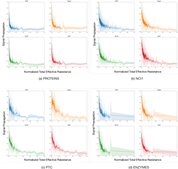
Figure 5: Decay of the amount of information propagated through the graphs w.r.t. the normalized total effective resistance (commute time) for: (a) $\mathsf{PROTEINS}$; (b) $\mathsf{NCI1}$; (c) $\mathsf{PTC}$; (d) $\mathsf{ENZYMES}$. For each dataset we report the decay for: (i) $\mathsf{GIN}$ (top-left); (ii) $\mathsf{Sage}$ (top-right), (iii) $\mathsf{GCN}$ (bottom-left) and (iv) $\mathsf{GAT}$(bottom-right).

In this section we provide synthetic experiments on the $\mathsf{PROTEINS}$, $\mathsf{NCI1}$, $\mathsf{PTC}$, $\mathsf{ENZYMES}$ datasets with the aim to provide empirical evidence to the fact that the total effective resistance of a graph, $\mathsf{Res}_{\mathsf{G}}=\sum_{v,u}\mathsf{Res}{(v,u)}$ (Ellens et al., 2011), is related to the ease of information propagation in an $\mathsf{MPNN}$. The experiment is designed as follows: we first fix a source node $v\in\mathsf{V}$ assigning it a $p$-dimensional unitary feature vector, and assigning the rest of the nodes zero-vectors. We then consider the quantity

$$h^{(m)}_{\odot}=\frac{1}{p\max_{u\neq v}d_{\mathsf{G}}(v,u)}\sum_{f=1}^{p}\sum_{u\neq v}\frac{h_{u}^{(m),f}}{\|h_{u}^{(m),f}\|}d_{\mathsf{G}}(v,u),$$

to be the amount of signal (or ‘information’) that has been propagated through $\mathsf{G}$ by an $\mathsf{MPNN}$ with $m$ layers. Intuitively, we measure the (normalized) propagation distance over $\mathsf{G}$, and average it over all the $p$ output channels. By propagation distance we mean the average distance to which the initial ‘unit mass’ has been propagated to - a larger propagation distance means that on average the unit mass has travelled further w.r.t. to the source node. The goal is to show that $h^{(m)}_{\odot}$ is inversely proportional to $\mathsf{Res}_{\mathsf{G}}$. In other words, we expect graphs with lower total effective resistance to have a larger propagation distance. The experiment is repeated for each graph $\mathsf{G}$ that belongs to the dataset $\mathcal{D}$. We start by randomly choosing the source node $v$, we then set $\mathbf{h}_{v}$ to be an arbitrary feature vector with unitary mass (i.e. $\|\mathbf{h}_{v}\|_{L_{1}}=1$) and assigning the zero-vector to all other nodes (i.e. $\mathbf{h}_{u}=\boldsymbol{0},\;u\neq v$). We use $\mathsf{MPNN}$s with a number of layers $m$ close to the average diameter of the graphs in the dataset, input and hidden dimensions $p=5$ and ReLU activations. In particular, we estimate the resistance of $\mathsf{G}$ by sampling $10$ nodes with uniform probability for each graph and we report $h^{(m)}_{\odot}$ accordingly. In Figure 5 we show that $\mathsf{MPNN}$s are able to propagate information further when the effective resistance is low, validating empirically the impact of the graph topology on over-squashing phenomena. It is worth to emphasize that in this experiment, the parameters of the $\mathsf{MPNN}$ are randomly initialized and there is no underlying training task. This implies that in this setup we are isolating the problem of propagating the signal throughout the graph, separating it from vanishing gradient phenomenon.

References

- Abboud et al. (2022) Abboud, R., Dimitrov, R., and Ceylan, I. I. Shortest path networks for graph property prediction. In The First Learning on Graphs Conference, 2022. URL https://openreview.net/forum?id=mWzWvMxuFg1.
- Abu-El-Haija et al. (2019) Abu-El-Haija, S., Perozzi, B., Kapoor, A., Alipourfard, N., Lerman, K., Harutyunyan, H., Ver Steeg, G., and Galstyan, A. Mixhop: Higher-order graph convolutional architectures via sparsified neighborhood mixing. In international conference on machine learning, pp. 21–29. PMLR, 2019.
- Alon & Yahav (2021) Alon, U. and Yahav, E. On the bottleneck of graph neural networks and its practical implications. In International Conference on Learning Representations, 2021.
- Arnaiz-Rodríguez et al. (2022) Arnaiz-Rodríguez, A., Begga, A., Escolano, F., and Oliver, N. DiffWire: Inductive Graph Rewiring via the Lovász Bound. In The First Learning on Graphs Conference, 2022. URL https://openreview.net/pdf?id=IXvfIex0mX6f.
- Banerjee et al. (2022) Banerjee, P. K., Karhadkar, K., Wang, Y. G., Alon, U., and Montúfar, G. Oversquashing in gnns through the lens of information contraction and graph expansion. In Annual Allerton Conference on Communication, Control, and Computing (Allerton), pp. 1–8. IEEE, 2022.
- Barceló et al. (2019) Barceló, P., Kostylev, E. V., Monet, M., Pérez, J., Reutter, J., and Silva, J. P. The logical expressiveness of graph neural networks. In International Conference on Learning Representations, 2019.
- Bartlett et al. (2017) Bartlett, P. L., Foster, D. J., and Telgarsky, M. J. Spectrally-normalized margin bounds for neural networks. Advances in neural information processing systems, 30, 2017.
- Bengio et al. (1994) Bengio, Y., Simard, P., and Frasconi, P. Learning long-term dependencies with gradient descent is difficult. IEEE transactions on neural networks, 5(2):157–166, 1994.
- Black et al. (2023) Black, M., Nayyeri, A., Wan, Z., and Wang, Y. Understanding oversquashing in gnns through the lens of effective resistance. arXiv preprint arXiv:2302.06835, 2023.
- Bodnar et al. (2021a) Bodnar, C., Frasca, F., Otter, N., Wang, Y., Lio, P., Montufar, G. F., and Bronstein, M. Weisfeiler and lehman go cellular: Cw networks. In Advances in Neural Information Processing Systems, volume 34, pp. 2625–2640, 2021a.
- Bodnar et al. (2021b) Bodnar, C., Frasca, F., Wang, Y., Otter, N., Montúfar, G. F., Lió, P., and Bronstein, M. M. Weisfeiler and lehman go topological: Message passing simplicial networks. In International Conference on Machine Learning, pp. 1026–1037, 2021b.
- Bodnar et al. (2022) Bodnar, C., Giovanni, F. D., Chamberlain, B. P., Lió, P., and Bronstein, M. M. Neural sheaf diffusion: A topological perspective on heterophily and oversmoothing in GNNs. In Advances in Neural Information Processing Systems, 2022.
- Bresson & Laurent (2017) Bresson, X. and Laurent, T. Residual gated graph convnets. arXiv preprint arXiv:1711.07553, 2017.
- Brüel-Gabrielsson et al. (2022) Brüel-Gabrielsson, R., Yurochkin, M., and Solomon, J. Rewiring with positional encodings for graph neural networks. arXiv preprint arXiv:2201.12674, 2022.
- Bruna et al. (2014) Bruna, J., Zaremba, W., Szlam, A., and LeCun, Y. Spectral networks and locally connected networks on graphs. In International Conference on Learning Representations, 2014.
- Cai & Wang (2020) Cai, C. and Wang, Y. A note on over-smoothing for graph neural networks. arXiv preprint arXiv:2006.13318, 2020.
- Chandra et al. (1996) Chandra, A. K., Raghavan, P., Ruzzo, W. L., Smolensky, R., and Tiwari, P. The electrical resistance of a graph captures its commute and cover times. computational complexity, 6(4):312–340, 1996.
- Chen et al. (2020) Chen, Z., Li, L., and Bruna, J. Supervised community detection with line graph neural networks. In International conference on learning representations, 2020.
- Chung & Graham (1997) Chung, F. R. and Graham, F. C. Spectral graph theory. American Mathematical Soc., 1997.
- Dasoulas et al. (2021) Dasoulas, G., Lutzeyer, J. F., and Vazirgiannis, M. Learning parametrised graph shift operators. In International Conference on Learning Representations, 2021.
- Deac et al. (2022) Deac, A., Lackenby, M., and Veličković, P. Expander graph propagation. In The First Learning on Graphs Conference, 2022.
- Defferrard et al. (2016) Defferrard, M., Bresson, X., and Vandergheynst, P. Convolutional neural networks on graphs with fast localized spectral filtering. In Advances in neural information processing systems, volume 29, 2016.
- Devriendt & Lambiotte (2022) Devriendt, K. and Lambiotte, R. Discrete curvature on graphs from the effective resistance. Journal of Physics: Complexity, 2022.
- Di Giovanni et al. (2022a) Di Giovanni, F., Luise, G., and Bronstein, M. Heterogeneous manifolds for curvature-aware graph embedding. In International Conference on Learning Representations Workshop on Geometrical and Topological Representation Learning, 2022a.
- Di Giovanni et al. (2022b) Di Giovanni, F., Rowbottom, J., Chamberlain, B. P., Markovich, T., and Bronstein, M. M. Graph neural networks as gradient flows. arXiv preprint arXiv:2206.10991, 2022b.
- Dörfler et al. (2018) Dörfler, F., Simpson-Porco, J. W., and Bullo, F. Electrical networks and algebraic graph theory: Models, properties, and applications. Proceedings of the IEEE, 106(5):977–1005, 2018.
- Ellens et al. (2011) Ellens, W., Spieksma, F. M., Van Mieghem, P., Jamakovic, A., and Kooij, R. E. Effective graph resistance. Linear algebra and its applications, 435(10):2491–2506, 2011.
- Gilmer et al. (2017) Gilmer, J., Schoenholz, S. S., Riley, P. F., Vinyals, O., and Dahl, G. E. Neural message passing for quantum chemistry. In International Conference on Machine Learning, pp. 1263–1272. PMLR, 2017.
- Goller & Kuchler (1996) Goller, C. and Kuchler, A. Learning task-dependent distributed representations by backpropagation through structure. In Proceedings of International Conference on Neural Networks (ICNN’96), volume 1, pp. 347–352. IEEE, 1996.
- Gori et al. (2005) Gori, M., Monfardini, G., and Scarselli, F. A new model for learning in graph domains. In Proceedings. 2005 IEEE International Joint Conference on Neural Networks, 2005., volume 2, pp. 729–734. IEEE, 2005.
- Gutteridge et al. (2023) Gutteridge, B., Dong, X., Bronstein, M., and Di Giovanni, F. Drew: Dynamically rewired message passing with delay. arXiv preprint arXiv:2305.08018, 2023.
- Hamilton et al. (2017) Hamilton, W. L., Ying, R., and Leskovec, J. Inductive representation learning on large graphs. In Advances in Neural Information Processing Systems, pp. 1025–1035, 2017.
- Hochreiter & Schmidhuber (1997) Hochreiter, S. and Schmidhuber, J. Long short-term memory. Neural computation, 9(8):1735–1780, 1997.
- Jegelka (2022) Jegelka, S. Theory of graph neural networks: Representation and learning. arXiv preprint arXiv:2204.07697, 2022.
- Karhadkar et al. (2022) Karhadkar, K., Banerjee, P. K., and Montúfar, G. Fosr: First-order spectral rewiring for addressing oversquashing in gnns. arXiv preprint arXiv:2210.11790, 2022.
- Kawaguchi (2016) Kawaguchi, K. Deep learning without poor local minima. In Advances in neural information processing systems, volume 29, 2016.
- Kipf & Welling (2017) Kipf, T. N. and Welling, M. Semi-Supervised Classification with Graph Convolutional Networks. In International Conference on Learning Representations, 2017.
- Klicpera et al. (2019) Klicpera, J., Weissenberger, S., and Günnemann, S. Diffusion improves graph learning. In Advances in Neural Information Processing Systems, 2019.
- Kreuzer et al. (2021) Kreuzer, D., Beaini, D., Hamilton, W., Létourneau, V., and Tossou, P. Rethinking graph transformers with spectral attention. In Advances in Neural Information Processing Systems, volume 34, pp. 21618–21629, 2021.
- Li et al. (2019) Li, G., Muller, M., Thabet, A., and Ghanem, B. Deepgcns: Can gcns go as deep as cnns? In Proceedings of the IEEE/CVF international conference on computer vision, pp. 9267–9276, 2019.
- Li et al. (2021) Li, G., Müller, M., Ghanem, B., and Koltun, V. Training graph neural networks with 1000 layers. In International conference on machine learning, pp. 6437–6449. PMLR, 2021.
- Lovász (1993) Lovász, L. Random walks on graphs. Combinatorics, Paul erdos is eighty, 2(1-46):4, 1993.
- Ma et al. (2020) Ma, Z., Xuan, J., Wang, Y. G., Li, M., and Liò, P. Path integral based convolution and pooling for graph neural networks. In Advances in Neural Information Processing Systems, volume 33, pp. 16421–16433, 2020.
- Mialon et al. (2021) Mialon, G., Chen, D., Selosse, M., and Mairal, J. Graphit: Encoding graph structure in transformers. CoRR, abs/2106.05667, 2021.
- Morris et al. (2019) Morris, C., Ritzert, M., Fey, M., Hamilton, W. L., Lenssen, J. E., Rattan, G., and Grohe, M. Weisfeiler and leman go neural: Higher-order graph neural networks. In AAAI Conference on Artificial Intelligence, pp. 4602–4609. AAAI Press, 2019.
- Nikolentzos et al. (2020) Nikolentzos, G., Dasoulas, G., and Vazirgiannis, M. k-hop graph neural networks. Neural Networks, 130:195–205, 2020.
- Nt & Maehara (2019) Nt, H. and Maehara, T. Revisiting graph neural networks: All we have is low-pass filters. arXiv preprint arXiv:1905.09550, 2019.
- Ollivier (2007) Ollivier, Y. Ricci curvature of metric spaces. Comptes Rendus Mathematique, 345(11):643–646, 2007.
- Ollivier (2009) Ollivier, Y. Ricci curvature of markov chains on metric spaces. Journal of Functional Analysis, 256(3):810–864, 2009.
- Pascanu et al. (2013) Pascanu, R., Mikolov, T., and Bengio, Y. On the difficulty of training recurrent neural networks. In International conference on machine learning, pp. 1310–1318. PMLR, 2013.
- Rampasek et al. (2022) Rampasek, L., Galkin, M., Dwivedi, V. P., Luu, A. T., Wolf, G., and Beaini, D. Recipe for a general, powerful, scalable graph transformer. In Advances in Neural Information Processing Systems, 2022.
- Ruiz et al. (2020) Ruiz, L., Gama, F., and Ribeiro, A. Gated graph recurrent neural networks. IEEE Transactions on Signal Processing, 68:6303–6318, 2020.
- Rusch & Mishra (2021a) Rusch, T. K. and Mishra, S. Coupled oscillatory recurrent neural network (co{rnn}): An accurate and (gradient) stable architecture for learning long time dependencies. In International Conference on Learning Representations, 2021a. URL https://openreview.net/forum?id=F3s69XzWOia.
- Rusch & Mishra (2021b) Rusch, T. K. and Mishra, S. Unicornn: A recurrent model for learning very long time dependencies. In International Conference on Machine Learning, pp. 9168–9178. PMLR, 2021b.
- Rusch et al. (2022) Rusch, T. K., Chamberlain, B. P., Rowbottom, J., Mishra, S., and Bronstein, M. M. Graph-coupled oscillator networks. In International Conference on Machine Learning, 2022.
- Scarselli et al. (2008) Scarselli, F., Gori, M., Tsoi, A. C., Hagenbuchner, M., and Monfardini, G. The graph neural network model. IEEE transactions on neural networks, 20(1):61–80, 2008.
- Sperduti (1993) Sperduti, A. Encoding labeled graphs by labeling raam. In Advances in Neural Information Processing Systems, volume 6, 1993.
- Thomassen (1990) Thomassen, C. Resistances and currents in infinite electrical networks. Journal of Combinatorial Theory, Series B, 49(1):87–102, 1990.
- Topping et al. (2022) Topping, J., Di Giovanni, F., Chamberlain, B. P., Dong, X., and Bronstein, M. M. Understanding over-squashing and bottlenecks on graphs via curvature. In International Conference on Learning Representations, 2022.
- Velingker et al. (2022) Velingker, A., Sinop, A. K., Ktena, I., Veličković, P., and Gollapudi, S. Affinity-aware graph networks. arXiv preprint arXiv:2206.11941, 2022.
- Veličković et al. (2018) Veličković, P., Cucurull, G., Casanova, A., Romero, A., Liò, P., and Bengio, Y. Graph attention networks. In International Conference on Learning Representations, 2018.
- Wang et al. (2020) Wang, G., Ying, R., Huang, J., and Leskovec, J. Multi-hop attention graph neural network. arXiv preprint arXiv:2009.14332, 2020.
- Xu et al. (2018) Xu, K., Li, C., Tian, Y., Sonobe, T., Kawarabayashi, K.-i., and Jegelka, S. Representation learning on graphs with jumping knowledge networks. In International Conference on Machine Learning, pp. 5453–5462. PMLR, 2018.
- Xu et al. (2019) Xu, K., Hu, W., Leskovec, J., and Jegelka, S. How powerful are graph neural networks? In International Conference on Learning Representations, 2019.
- Ying et al. (2021) Ying, C., Cai, T., Luo, S., Zheng, S., Ke, G., He, D., Shen, Y., and Liu, T.-Y. Do transformers really perform badly for graph representation? In Advances in Neural Information Processing Systems, volume 34, pp. 28877–28888, 2021.
- Zhao et al. (2022) Zhao, W., Wang, C., Han, C., and Guo, T. Analysis of graph neural networks with theory of markov chains. 2022.