Optimisation of time-ordered processes in the finite and asymptotic regime

Abstract

Many problems in quantum information theory can be formulated as optimizations over the sequential outcomes of dynamical systems subject to unpredictable external influences. Such problems include many-body entanglement detection through adaptive measurements, computing the maximum average score of a preparation game over a continuous set of target states and limiting the behavior of a (quantum) finite-state automaton. In this work, we introduce tractable relaxations of this class of optimization problems. To illustrate their performance, we use them to: (a) compute the probability that a finite-state automaton outputs a given sequence of bits; (b) develop a new many-body entanglement detection protocol; (c) let the computer invent an adaptive protocol for magic state detection. As we further show, the maximum score of a sequential problem in the limit of infinitely many time-steps is in general incomputable. Nonetheless, we provide general heuristics to bound this quantity and show that they provide useful estimates in relevant scenarios.

I Introduction

In quantum physics we are usually concerned with manipulating quantum systems, whether we interact with them to cause them to reach (or remain in) a specific quantum state, or measure them in order to observe or certify some of their properties. Finding new, better ways to perform tasks with time-ordered operations lies at the heart of current research in quantum information science. Quantum computing relies on a sequential application of gates to a quantum system and communication protocols aided by quantum systems depend on performing operations on these systems and exchanging information in a specific order. Sequences of operations are also crucial in less evident situations, for instance specific sequences of pulses are applied in order to readout a superconducting qubit [47].

Traditionally, the problem of finding new ways (or sequences of operations) to complete a specific task has been dependent on the ingenuity of scientists to come up with new protocols. More recently, this type of problem is also tackled via machine learning techniques, which require training a neural network to generate the right sequence of operations. However, a general method to optimise over sequential strategies or even a criterion to decide whether one such sequential protocol is optimal for a certain task is lacking.

Part of the difficulty in solving these problems lies in the fact that, when operations are performed sequentially, protocols can be made adaptive, i.e. future operations may depend on the result of previous ones. Adaptiveness can lead to great advantages, e.g.: it minimises statistical errors in entanglement certification [48] and quantum state detection [16]. However, it also increases the variety of protocols that must be considered for a specific task, and thus the complexity of optimising over them. Indeed, while optimisation techniques are well-established in the context of single-shot or independently repeated procedures (e.g. in applications of non-locality [31, 32] or for witnessing entanglement [29]), developing them for sequential protocols remains a challenge.

In this work, we make progress on this problem. Specifically, we introduce a general technique to analyse and optimise a class of time-ordered processes that we call sequential models. These are protocols in $N$ rounds, where in each round an interaction occurs and changes the state of a system of interest possibly depending on unknown or uncontrolled variables. The progress towards a certain goal is quantified by a reward that is generated at each round of the protocol and is the object of our optimization procedure.

Our first result is a technique that allows us to upper bound the maximum total reward that a sequential model can generate in $N$ rounds through a complete hierarchy of increasingly difficult convex optimization problems. To illustrate the performance of the hierarchy, we apply it to upper bound the type-I error of an adaptive protocol for many-body entanglement detection [39, 48]. The technique generates seemingly tight bounds for large system sizes (of order $N\approx 100$).

The same technique also allows us to deepen the study of temporal correlations generated by finite-state automata [35, 38]. These models appear in several problems in quantum foundations and quantum information theory such as classical simulations of quantum contextuality [22, 14, 6, 5], quantum simulations of classical stochastic processes [15, 11, 12], purity certification [41], dimension witnesses [19, 43, 42], quantum advantages in the design of time-keeping devices [13, 49, 7, 45], and classical simulation of quantum computation  [50]; see a recent review on temporal correlations for more details [46]. Specifically, we focus on the problem of optimal clocks, namely, how good a clock can we construct, given access to a classical automaton with $d$ internal states? Using our tools, we solve this problem for low values of $d$, by providing upper bounds on the maximum probability that the automaton outputs the ‘one-tick sequence’ $000...01$ investigated in [7, 45]. These bounds match the best known lower bounds up to numerical precision.

In addition to finite sequences of operations, we are also often interested in letting a protocol or process run indefinitely, i.e., we are interested in characterising its asymptotic behaviour as $N\rightarrow\infty$. This is for instance important for systems that are left to evolve for a long time or in cases where we aim to probe large systems, where this limit is a good approximation.

To our knowledge, not much is known about time-ordered processes in the limit of infinitely many rounds (except for results on asymptotic rates in hypothesis testing and when taking specific limits [3, 26]). In this paper we show that there is a fundamental reason for this: there are sequential models for which no algorithm can approximate their asymptotic behaviour. This follows from undecidability results related to finite state automata, specifically a construction from [18, 10]. Nevertheless, we develop a heuristic method for computing rigorous bounds on the asymptotic behaviour. We further find that, in the applications we consider, these bounds are close to the expected asymptotic behaviour and to the lower bounds we can compute, thus substantiating the usefulness of our method. More specifically, we use the asymptotic method to bound the type-I error of the many-body entanglement detection protocol mentioned above in the limit of infinitely many particles. The result is a bound that is, at most, at a distance of $4\cdot 10^{-4}$ from the actual figure. Our asymptotic method also bounds the probability that a two-state automaton outputs the one-tick sequence in the limit of many time-steps to $O(10^{-2})$.

Finally, in some circumstances it becomes necessary, not to analyze, but to find sequential models with a good performance. That is, given a number of parameters that we can control – the policy –, which might affect the system’s evolution as well as the reward, we pose the problem of deciding which policy maximizes the total reward after $N$ rounds. We propose to tackle this problem via projected gradient methods, and show how to cast the computation of the gradient of our upper bounds as a tractable convex optimization problem. Using this approach, we let the computer discover a $2$-state, $6$-round preparation game to detect one-qubit magic states.

Our article is structured as follows. In Section II, we present three problems in quantum information theory that we will use to illustrate our methods throughout. In Section III, we introduce the abstract notion of sequential models and show how to optimise them, before applying the optimisation method in Section IV. In Section V, we prove that the asymptotic behaviour of sequential models cannot be approximated in general. We also introduce a heuristic to tackle asymptotic problems, which we apply in Section VI. In section VII, we pose the problem of policy optimization and show how to compute the gradient of the upper bounds derived in section III, over the parameters of the policy. We use gradient methods to solve a policy optimization problem in section VIII. Finally, we present our conclusions in Section IX.

II Problems with time-ordered operations

A variety of different problems involving quantum systems are of a sequential nature. In the following we introduce three settings that are made up of time-ordered operations and that all pose challenging open problems to the quantum information community.

II.1 Temporal correlations

A finite-state automaton (FSA) is a mathematical structure that models an autonomous computational device with bounded memory. More formally [35, 38], a $d$-state automaton is a device described, at every time, by an internal state $\sigma\in\Sigma$, with $|\Sigma|=d$. At regular intervals, rounds or time-steps, the automaton updates its internal state and generates an outcome $b\in B$, depending on both its prior internal state $\sigma$ and the state $y\in Y$ of its input port. Such a double state-and-output transition is governed by the automaton’s transition matrix $P(\sigma^{\prime},b|\sigma,y)$, which indicates the probability that the automaton transitions to the internal state $\sigma^{\prime}$ and outputs $b$, given that its input and prior states were, respectively, $y,\sigma$. Overall, the probability of outputs $b_{1},\ldots,b_{n}$ given inputs $y_{1},\ldots,y_{n}$ can be computed as

$$p(b_{1},\ldots,b_{n}|y_{1},\ldots,y_{n})=\sum_{\sigma_{0},\sigma_{1},\ldots,\sigma_{n}}p(\sigma_{0})P(\sigma_{1},b_{1}|\sigma_{0},y_{1})P(\sigma_{2},b_{2}|\sigma_{1},y_{2})\ldots P(\sigma_{n},b_{n}|\sigma_{n-1},y_{n})$$ (1)

Expressions such as Eq. (1), i.e., generated by a classical FSA, appear in several problems related to classical simulations of temporal quantum correlations, such as, e.g., classical simulations of quantum contextuality [22, 14, 6], quantum simulations of classical stochastic processes [15, 11, 12], quantum advantages in the design of time-keeping devices [13, 49, 7, 45], and classical simulation of quantum computation  [50].

We are interested in scenarios where the performance of a $d$-state automaton after $n$ time-steps is evaluated by yet another automaton, or, more generally, by a time-dependent process with bounded memory. We wish to bound said performance over all automata with $d$ states.

Consider thus a FSA $A$, with states denoted by $\sigma\in\Sigma$, with $|\Sigma|=d$, inputs $y\in Y$ and outputs $b\in B$. We assume that the automaton is described by the (unknown) transition matrix $P(\sigma_{k+1},b_{k}|\sigma_{k},y_{k})$. Let $Q$ be a known time-dependent process, with internal state denoted by $t$, and inputs (outputs) denoted by $z$ ($c$). The (known) transition matrix of this process at time-steps $k=2,...,N$ is $Q_{k}(t_{k},c_{k}|t_{k-1},z_{k-1})$. Each state $t_{k}$ of the process is associated with a reward $\alpha_{k}(t_{k})$. At time-step $1$, state and output $t_{1},c_{1}$ are generated by the distribution $Q_{1}(t_{1},c_{1})$. Now, let us couple $Q$ with $A$, in the following way (see also Figure 1 for an illustration): after $Q$ generates $t_{1},c_{1}$, we input $c_{1}$ in the automaton $A$, i.e., we let $y_{1}=c_{1}$. The automaton then transitions through $P$ to a state $\sigma_{1}$, outputting $b_{1}$. This output is further input into the process $Q$ (by letting $z_{1}=b_{1}$), which in turn generates $t_{2},c_{2}$ through $Q_{2}$, and so on. At time-step $N$ we consider the sum of all rewards

$$\sum_{k=1}^{N}\alpha_{k}(t_{k}).$$ (2)

Our goal is to maximize the expectation value of the total reward over all $d$-state automata $A$.

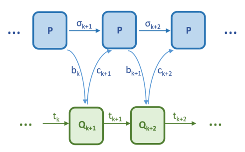
Figure 1: Automaton (blue) coupled to a process $Q$ (green). The process may in general differ from round to round.

Note that by convexity, the best strategy is for the automaton to be initialized in a specific state $\sigma_{0}=\bar{\sigma}_{0}$ rather than a distribution thereof. Hence, fixing the initial state, the optimal automaton is fully characterised in terms of the transition matrix $P$ that maximizes the expected reward.

This problem can be mathematically rephrased in a way that will prove useful later. Namely, the coupled systems $A$, $Q$ can be regarded as a single dynamical system whose internal state $s_{k}$ at time-step $k$ corresponds to the probability distribution of the triple $(t_{k},c_{k},\sigma_{k})$, i.e., $s_{k}:=p_{k}(t_{k},c_{k},\sigma_{k})$. The evolution of this system from one time-step to the next follows the equation of motion

$$p_{k+1}(t_{k+1},c_{k+1},\sigma_{k+1})=\sum_{c_{k},t_{k},\sigma_{k},b_{k}}p_{k}(t_{k},c_{k},\sigma_{k})P(\sigma_{k+1},b_{k}|\sigma_{k},c_{k})Q_{k+1}(t_{k+1},c_{k+1}|t_{k},b_{k})=:f_{k}(s_{k},\lambda).$$ (3)

Note that the evolution is here given by a polynomial $f_{k}$ of the state $s_{k}$ and an unknown evolution parameter $\lambda:=(P(\sigma^{\prime},c|\sigma,z):z\in Z,c\in C,\sigma\in\Sigma)$. In this formulation of the problem, the reward $r_{k}$ at time-step $k$ is given by

$$r_{k}(s_{k}):=\sum_{t_{k},c_{k},\sigma_{k}}p_{k}(t_{k},c_{k},\sigma_{k})\alpha(t_{k}).$$ (4)

Notice that the reward does not depend on $\lambda$ here (except via the $p_{k}$), such a dependency could, however, be introduced by using different reward functions $r_{k}(s_{k},\lambda)$. In this picture, our task is to maximize the total reward over all possible evolution parameters $\lambda$.

II.2 Entanglement certification of many-body systems

Given an $N$-partite quantum system, we are often faced with the problem of determining whether its state is entangled. In principle, this problem can be solved by finding an appropriate entanglement witness and estimating its value on the state at hand. However, in addition to the problem that finding such a witness theoretically is NP-hard [17], its estimation may involve conducting joint measurements on many subsystems of the $N$-partite state, a feat that may not be experimentally possible. Replacing such joint measurements by estimates based on local measurement statistics requires, in general, $\mbox{Exp}[N]$ state preparations, thus rendering the corresponding protocols infeasible for moderately sized $N$ (as is the case when the protocol demands full quantum state tomography).

One way to avoid these problems, i.e. perform single-system measurements and reduce the number of state preparations, is carrying out an adaptive protocol [48]. Such a scheme proceeds as follows: we sequentially measure the particles that constitute the $N$-particle ensemble, making future measurements depend on previous ones as well as on previous outcomes. Once we conduct the last measurement, we make a guess on whether the underlying state was entangled or not.

To choose how to measure each system and to make our final guess, we use a dynamical system $Q$. This process has internal states $t_{k}\in T$, and its transition matrix at time $k=1,...,N-1$ is of the form $Q_{k}(t_{k+1},y_{k+1}|t_{k},b_{k})$, where $b_{k}\in B$ denotes the measurement outcome at time $k$ and $y_{k+1}$ labels the measurements to be conducted on the $(k+1)^{th}$ particle. For each $y\in Y_{k}$, there exists a Positive Operator Valued Measure (POVM) $\{M^{k}_{b|y}\}_{b}$. The final guess is generated through the function $Q_{N}(t_{N+1}|t_{N},b_{N})$, with $t_{N+1}\in\{\mbox{`entangled', `separable'}\}$. The initial state of the process and the measurement setting $y_{1}$ for the first particle are generated by the distribution $Q_{0}(t_{1},y_{1})$. This is illustrated in Figure 2.

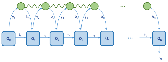
Figure 2: Sequential model for entanglement detection. The particles of an $N$-party state (green) are measured one by one. The $k$-th measurement $y_{k}$ depends on the internal state of a finite state automaton, the outcome $b_{k}$ affects the transition of the automaton according to $Q_{k}$.

If the target state $\rho$ whose entanglement we wish to detect experimentally admits a Matrix Product Operator (MPO) decompositon [28], then one can efficiently compute the probability that the process outputs the result ‘separable’, see Figure 3. This probability is usually called a type-II error, or a “false negative”.

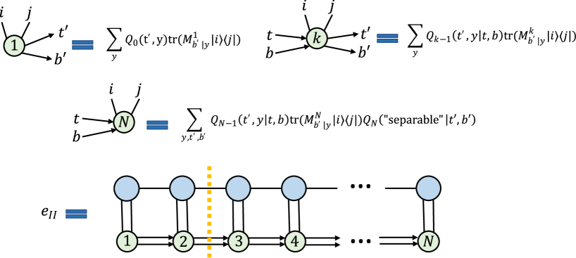
Figure 3: Efficient computation of the type-II error. The blue circles represent the tensors making up our MPO target state, with two vertical legs denoting the bra and ket indices of each particle and two horizontal legs of dimension $D$ –the bond dimension– to account for the target state’s correlations. Defining the green tensors in the way indicated in the figure, their contraction with the blue tensors equals the type-II error of the corresponding entanglement detection protocol. This contraction can be computed by multiplying matrices of dimension $|T||B|D$, as the dashed orange line indicates.

It remains to compute the type-I error, or “false positive” of the entanglement detection protocol encoded in $Q$: that would correspond to the maximum probability that the process outputs ‘entangled’ when the input is a fully separable quantum state. In computing this maximum, we can assume, by convexity, that the player has prepared a pure product quantum state. That is, at each time-step $k$, we measure some pure quantum state $\rho_{k}$. Despite this simplification, computing the type-I error of the scheme requires maximizing a multi-linear function with a size-$O(N)$ input. As $N$ grows, this becomes a more difficult problem.

Like the problem of computing the maximum performance over all $d$-state automata, maximizing the type-I error over the set of separable states can be phrased as an optimization over the sequential outputs of a deterministic dynamical system. In this case, the dynamical system’s internal state $s_{k}$ at time-step $k$ would correspond to the distribution $P_{k}$ of $t_{k},y_{k}$. The system’s equation of motion is

$$P_{k+1}(t_{k+1},y_{k+1})=\sum_{t_{k},y_{k},b_{k}}P_{k}(t_{k},y_{k})\mbox{tr}(M^{k}_{b_{k}|y_{k}}\rho_{k})Q_{k}(t_{k+1},y_{k+1}|t_{k},b_{k}),$$ (5)

where the quantum state $\rho_{k}$ can be interpreted as an uncontrolled external variable $h$ influencing the evolution of the system. At time-step $N$, the system outputs the deterministic outcome

$$r_{N}(s_{N})=\sum_{t_{N},y_{N},b_{N}}P_{N}(t_{N},y_{N})\mbox{tr}(M^{N}_{b_{N}|y_{N}}\rho_{N})Q_{N}(t_{N+1}|t_{N},b_{N})\delta_{t_{N+1},\mbox{`entangled'}}.$$ (6)

II.3 Independent and identically distributed (i.i.d) preparation strategies in quantum preparation games

The notion of preparation games aims to capture the structure of general (possibly adaptive) protocols, where quantum systems are probed sequentially [48]. More precisely, a quantum preparation game is an $N$-round task involving a player and a referee. In each round, the player prepares a quantum state, which is then probed by the referee. In round $k$, before carrying out his measurement, the referee’s current knowledge of the source used by the player is encoded in a variable $t_{k}\in T_{k}$, with $|T_{k}|<\infty$, called the game configuration. This variable depends non-trivially on the past history of measurements and measurement results: in each round, it guides the referee in deciding which measurement to perform next and changes depending on its outcome. This double role of the game configuration can be encoded in the POVM used by the referee for that round. That is, assuming that the game configuration before the measurement is $t\in T_{k}$, the probability that the new game configuration is $t^{\prime}\in T_{k+1}$ is given by $\mbox{tr}(\rho_{k}M^{k}_{t^{\prime}|t})$, where $\rho_{k}$ is the player’s $k^{th}$ state preparation; and $\{M^{k}_{t^{\prime}|t}:t^{\prime}\in T_{k+1}\}$, the POVM implemented by the referee when the game configuration is $t$. At the end of the preparation game, a score $g(t_{N+1})$, where $t_{N+1}$ denotes the final game configuration, is generated by the referee according to some scoring system $g(t)$ for $t\in T_{N+1}$.

In some circumstances, for instance in an entanglement detection protocol where the player tries to (honestly) prepare a specific entangled state, it makes sense to consider a player that follows an independent and identically distributed (i.i.d.) strategy, meaning that the player produces the same state $\rho$ in each round.

Consider thus the problem of computing the maximum game score, for a fixed scoring system, achievable with preparation strategies of the form $\rho^{\otimes n}$, with $\rho\in C$, where $C$ is some set of states. In [48], it was shown how to compute the maximum score of a preparation game under i.i.d. strategies when the set $C$ of feasible preparations has finite cardinality. In this work, we consider the case where $C$ is continuous.

This problem can be modeled through a dynamical system whose internal state $s_{k}$ at time $k$ corresponds to $P_{k}(t_{k})$, the distribution of game configurations at the beginning of round $k$. The system’s equation of motion is

$$P_{k+1}(t^{\prime})=\sum_{t\in T_{k}}P_{k}(t)\mbox{tr}(\rho M^{k}_{t^{\prime}|t}),$$ (7)

where the unknown evolution parameters $\lambda:=\rho\in C$ correspond to the player’s preparation. The dynamical system outputs a reward at time $N$, namely

$$r_{N}(s_{N},\lambda)=\sum_{t^{\prime}\in T_{N+1}}g(t^{\prime})\sum_{t\in T_{k}}P_{N}(t)\mbox{tr}(\rho M^{N}_{t^{\prime}|t}).$$ (8)

Our goal is thus to maximize the system’s reward over all possible values of the evolution parameter $\lambda$, i.e., over all $\rho\in C$.

As an aside we note that, in some circumstances, it becomes necessary to compute the maximum average game score achievable by an adversarial player, who has access to the current game configuration and can thus adjust their preparation in each round accordingly. Curiously enough, this problem is easier than optimizing over i.i.d. strategies, and, in fact, a general solution is presented in [48]. Notwithstanding, we show below that the computation of the maximum game score of a preparation game under adaptive strategies can also be regarded as a particular class of the sequential problems considered in this article.

III Sequential models and their optimisation

The three problems described above are – even though from a physical point of view rather different – structurally very similar. Indeed, they are all examples of the type of problem that we introduce more abstractly in the following. Consider a scenario where the state of a dynamical system is fully described at time-step $k$ by a variable $s_{k}\in S_{k}$. Between time-steps $k$ and $k+1$, the system transitions from $s_{k}$ to another state $s_{k+1}$ depending on $s_{k}$, a number of uncontrolled variables $h_{k}\in H_{k}$ and a number of unknown evolution parameters $\lambda\in\Lambda$. The equation of motion that describes this transition is

$$s_{k+1}=f_{k}(s_{k},h_{k},\lambda),$$ (9)

where $S_{k}$, $H_{k}\ \forall k$ and $\Lambda$ are sets of parameter values.

Our goal is to optimise over this type of system, according to some figure of merit that is given by the problem at hand. We model this by assuming that, in each time-step, the system emits a reward (or penalty) $r_{k}(s_{k},h_{k},\lambda)$. Notice that this reward may be the zero function for certain $k$, so that this includes problems where only the final outcome matters as a special case. We shall refer to such a system from now on as a sequential model, see Figure 4.

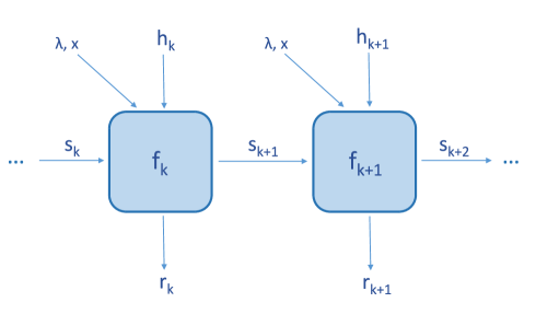
Figure 4: Pictorial representation of a sequential model. Notice that the equation of motion itself may capture several interactions or be composed of several steps (e.g. the measurement of a quantum system followed by the update of a finite state automaton).

Our goal is to estimate the maximum total reward $\nu^{\star}$ over all possible values of $\lambda,h_{1},...,h_{N}$. That is, we wish to solve the problem

$$\nu^{\star}\ :=\ \max_{\lambda,h}\quad \sum_{k=1}^{N}r_{k}(s_{k},h_{k},\lambda)$$

such that $$\lambda\in\Lambda,\ h\in\times_{k=1}^{N}H_{k}$$ (10)

$$s_{k+1}=f_{k}(s_{k},h_{k},\lambda)\ \ \forall k.$$

We generally assume that the initial state $s_{1}$ is known; otherwise, we can absorb it into the definition of $\lambda$ in the sense that we add one time-step that generates the initial state. In the absence of $\lambda$, the above is mathematically equivalent to a deterministic Markov decision problem, if we regard $h$ as an action [36].

III.1 Reformulation of the optimisation over sequential models

To compute the optimal value $\nu^{\star}$, we consider an approach based on dynamical programming methods [36]. It consists in defining value functions $V_{k}(s_{k},\lambda)$, which represent the maximum reward achievable between time-steps $k$ and $N$ over all possible values of $h_{k},...,h_{N}$, starting from the state $s_{k}$, and under the assumption that the evolution parameters take the value $\lambda$. In terms of the reward functions, they are thus given by

$$V_{N}(s_{N},\lambda) =\max_{h_{N}\in H_{N}}r_{N}(s_{N},h_{N},\lambda),$$

$$V_{k}(s_{k},\lambda) =\max_{h_{k}\in H_{k}}r_{k}(s_{k},h_{k},\lambda)+V_{k+1}(f_{k}(s_{k},h,\lambda),\lambda)$$ (11)

and where we recover $\nu^{\star}$ in the final step as

$$\nu^{\star}=\max_{\lambda\in\Lambda}V_{1}(s_{1},\lambda).$$ (12)

The problem of finding $\nu^{\star}$ can thus be reduced to

$$\min_{V_{1},...,V_{N},\nu}\ \ \nu$$

such that $$V_{N}(s_{N},\lambda)\geq r_{N}(s_{N},h,\lambda)\quad\forall h\in H_{N},\ s_{N}\in S_{N},\ \lambda\in\Lambda$$

$$V_{k}(s_{k},\lambda)\geq r_{k}(s_{k},h,\lambda)+V_{k+1}(f_{k}(s_{k},h,\lambda),\lambda)\quad\forall h\in H_{k},\ s_{k}\in S_{k},\ \lambda\in\Lambda$$ (13)

$$\nu\geq V_{1}(s_{1},\lambda)\quad\forall\lambda\in\Lambda.$$

Indeed, on one hand, any feasible point of problem (13) provides an upper bound on $\nu^{\star}$. On the other hand, the $V_{1},...,V_{N},\nu^{\star}$, as defined by eqs. (11), (12), are also a feasible point of (13). Hence the solution of problem (13) is $\nu^{\star}$.

Unfortunately, unless their domain is finite, there is no general method for optimization over arbitrary functions. What is feasible is to solve problem (13) under the assumption that $\{V_{k}(s_{k},\lambda)\}_{k}$ belong to a class of functions ${\cal F}$ described by finitely many parameters. Since, in general, the optimal functions $V_{k}(s_{k},\lambda)$ might not belong to ${\cal F}$, the result $\bar{\nu}$ of such an optimization is an upper bound on the actual solution $\nu^{\star}$ of the problem. The class ${\cal F}$ of polynomial functions is very handy, as it is closed under composition and dense in the set of continuous functions with respect to the uniform norm. This is the class we are working on in this paper.

For the rest of the paper, we thus assume that, for all $k\in\{1,2,\ldots,N\}$, $f_{k}(s_{k},h_{k},\lambda),r_{k}(s_{k},h_{k},\lambda)$ are polynomials on $s_{k},h_{k},\lambda$, and that the sets $S,H_{k},\Lambda$ are bounded sets in some metric space that can be described by a finite number of polynomial inequalities. Note that, under these assumptions, the value functions are continuous on $s_{k},\lambda$.

Call then $\nu^{n}\geq\nu^{\star}$ the result of (13) under the constraint that $\{V_{k}(s_{k},\lambda)\}_{k}$ are polynomials of a given degree $n$. Since any continuous function defined on a bounded set can be arbitrarily well approximated by polynomials, it follows that $\lim_{n\to\infty}{\nu}^{n}=\nu^{\star}$.

There is the added difficulty that solving (13) entails enforcing positivity constraints of the form

$$p(x)\geq 0,\forall x\in X,$$ (14)

where $p(x)$ is a polynomial on the vector variable $x\in\mathbb{R}^{m}$ and $X$ is a bounded region of $\mathbb{R}^{m}$ defined by a finite number of polynomial inequalities (namely, a basic semialgebraic set). Fortunately, there exist several complete (infinite) hierarchies of sufficient criteria to prove the positivity of a polynomial on a semialgebraic set [23, 24, 40, 37]. In algebraic geometry, any such hierarchy of criteria is called a positivstellensatz.

Two prominent positivstellensätze are Schmüdgen’s [40] and Putinar’s [37]. Both hierarchies have the peculiarity that, for a fixed index $k$, the set of all polynomials satisfying the $k^{th}$ criterion is representable through a semidefinite program (SDP). The application of Schmüdgen’s and Putinar’s positivstellensätze for polynomial optimization thus leads to two complete hierarchies of SDP relaxations. The SDP relaxation based on Putinar’s positivstellensatz is known as the Lasserre-Parrilo hierarchy [25, 34]. The reader can find a description of both hierarchies in Appendix A. While the hierarchy based on Schmüdgen’s positivstellensatz is more computationally demanding than the Lasserre-Parrilo hierarchy, it converges faster. In our numerical calculations below, we use a hybrid of the two.

The use of the $k^{th}$ (sufficient) positivity test of a given positivstellensatz while optimizing over polynomial value functions of degree $n$ results in an upper bound $\nu^{n}_{k}$ on $\nu^{n}$, with $\lim_{k\to\infty}\nu^{n}_{k}=\nu^{n}$. For our purposes, the take-home message is that $\nu^{n}_{k}\geq\nu^{\star}$, for all $k,n$ and $\lim_{n\to\infty}\lim_{k\to\infty}\nu^{n}_{k}=\nu^{\star}$.

We finish this section by noting that there is nothing fundamental about the use of polynomials to approximate value functions. In fact, there exist other complete families of functions that one might utilize to solve problem (13). A promising such class is the set of signomials, or linear combinations of exponentials, for which there also exists a number of positivsellensätze in the literature [30, 9]. In this case, the corresponding sets of positive polynomials are not SDP representable, but are nonetheless tractable convex sets. As such, they are suitable for optimization.

III.2 Quantum preparation games as sequential models

Sequential models capture the structure of various types of time-ordered processes, including the three introduced in Section II. Here, we argue that sequential models are actually rather general: optimizations over adversarial strategies in quantum preparation games can be modeled as sequential problems, too. In fact, their resolution by means of value functions allows one to re-derive previous results on the topic [48].

Let ${\cal S}$ be a set of quantum states and consider a preparation game where the player is allowed to prepare, at each round $k$, any state $\rho(t_{k})\in{\cal S}$ depending on the current game configuration $t_{k}$. This preparation game can be interpreted as sequential model with $\Lambda=\emptyset$, $s_{k}=p_{k}(t_{k})$, $h_{k}=(\rho^{k}(t):t\in T_{k})$ and equation of motion

$$p_{k+1}(t^{\prime})=\sum_{t\in T_{k}}p_{k}(t)\mbox{tr}(\rho^{k}(t)M^{k}_{t^{\prime}|t}).$$ (15)

We consider the problem of maximizing the average game score (or reward)

$$r_{N+1}(p_{N+1})=\sum_{t\in T_{N+1}}p_{N+1}(t)g(t),$$ (16)

where $g$ is the game’s score function [48].

In principle, we could formulate this problem as (13). Note that $V_{N+1}=r_{N+1}$ is linear in $p_{N+1}$. This motivates us to consider an ansatz of linear value functions $V_{k}(p_{k})$ for this problem. That is, we aim to solve (13) under the assumption that

$$V_{k}(p_{k})=\sum_{t\in T_{k}}\mu_{k}(t)p_{k}(t),$$ (17)

for some vector $(\mu_{k}(t):t\in T_{k})$. The condition $V_{k}(p_{k})\geq V_{k+1}(p_{k+1})$ then translates to

$$\sum_{t\in T_{k}}\mu_{k}(t)p_{k}(t) \geq\max_{\{\rho^{k}(t)\}_{t}}\sum_{t^{\prime}\in T_{k+1}}\mu_{k+1}(t^{\prime})\sum_{t\in T_{k}}p_{k}(t)\mbox{tr}(\rho^{k}(t)M^{k}_{t^{\prime}|t})$$

$$=\sum_{t\in T_{k}}p_{k}(t)\max_{\rho^{k}(t)}\mbox{tr}\left(\rho^{k}(t)\sum_{t^{\prime}\in T_{k+1}}V_{k+1}(t^{\prime})M^{k}_{t^{\prime}|t}\right).$$ (18)

Setting $p_{k}(t)=\delta_{t,j}$, for $j\in T_{k}$, we arrive at the recursion relations:

$$\mu_{N+1}(t)=g(t),$$

$$\mu_{k}(t)=\max_{\rho^{k}(t)}\mbox{tr}\left(\rho^{k}(t)\sum_{t^{\prime}\in T_{k+1}}\mu_{k+1}(t^{\prime})M^{k}_{t^{\prime}|t}\right),$$ (19)

which allow us to compute $V_{1}(t_{0})$. This quantity is, in principle, an upper bound on the actual solution of (13), because we enforced the extra constraint that the value functions are linear. The upper bound is, however, tight, as can be seen by computing the preparation game’s average score under the preparation strategy given by the maximizers $\bar{\rho}^{k}(t)$ of (19). In fact, all the above is but a complicated way to arrive at the recursion relations provided in [48] to compute the maximum score of a preparation game.

IV Application to optimising time-ordered processes

All the sequential problems considered in this work could in principle be solved (or at least approximated) through the straight-forward application of the Lasserre-Parrilo hierarchy [25, 34]. However, the degree of the polynomials in such problems grows linearly with the number of steps $N$, thus making the corresponding SDP intractable for more than a few iterations (e.g., for the problem treated in Section IV.1 below, this is the case for a sequence of length $L=7$). Our reformulation of the sequential optimisation problem as in (13), on the other hand, allows us to circumvent this issue and to optimise sequential models for much higher values of $N$.

IV.1 Optimizations over finite-state automata: Probability bounds

In this section, we investigate the maximum probability with which a classical FSA can generate a given output sequence. This problem has been extensively investigated for input-output sequences [6], as well as sequences with only inputs [7, 45]. In particular, we consider the so-called one-tick sequence, $00\ldots 01$, introduced in [7] in connection with the problem of optimal clocks. For a sequence of total length $L$, we use the compact notation $0^{L-1}1$. Here, we use the general techniques developed in Section III to tackle this problem. Note that this is an instance of the type of problem introduced in Section II.1.

Consider a $d$-state automaton without inputs and with binary outputs, i.e., $Y=\emptyset$, $B=\{0,1\}$. We wish to compute the maximum probability $P(L)$ that the automaton outputs the one-tick sequence $0^{L-1}1$, denoted $P_{\rm max}^{\rm d}(L)$. For this purpose, let us construct a simple process $Q$ that, coupled to the automaton, produces an expected reward that equals $P(0^{L-1}1)$. $Q$ has two internal states, i.e., $t_{k}\in\{0,1\}$ and no outputs ($C=\emptyset$). Its initial state is $t_{1}=1$, and its transition matrices are as follows:

$$Q_{k}(t_{k+1}|t_{k},b_{k}) =\delta_{t_{k+1},t_{k}(1-b_{k})},\mbox{ for }k=1,...,L-1,$$

$$Q_{L}(t_{L+1}|t_{L},b_{L}) =\delta_{t_{L+1},t_{L}b_{L}}.$$ (20)

For time-steps $k=1,...,L-1$, the process $Q$ therefore keeps being in state $1$ as long as the automaton outputs $0$’s; if the automaton outputs any $1$, the state of the process changes to $0$ and stays there until the end of the game. At time-step $L$, process $Q$ receives the output $b_{L}$. If $b_{L}=0$ or $t_{L}=0$, then $t_{L+1}=0$; otherwise, $t_{L+1}=1$. The probability that the automaton produces the sequence $0^{L-1}1$ thus corresponds to the probability that $t_{L+1}=1$. This corresponds to a reward function

$$\alpha_{k}(t_{k}) =0,\mbox{ for }k=1,...,L-1,$$

$$\alpha_{L+1}(t_{L+1}) =\delta_{t_{L+1},1}.$$ (21)

Using the techniques developed in Section III, we map this problem to a polynomial optimization problem. Due to the choice of reward (together with the process $Q$), we see that the only terms from the equation of motion (3) that contribute to the final reward are the ones with correct $b_{k}$. This allows a further simplification of the model.

First, let us redefine the internal states of the sequential model to be the vector

$$s_{k}=(p_{k}(t_{k}=1,\sigma_{k+1}))_{\sigma},$$ (22)

described by $d$ parameters $s_{k}^{\sigma}$, with constraints $s_{k}^{\sigma}\geq 0$ for $\sigma=0,\ldots,d-1$, and $1-\sum_{\sigma}s_{k}^{\sigma}\geq 0$. Next, we redefine the unknown evolution parameter $\lambda$ to have dimension $d^{2}$, through: $\lambda:=(P(\sigma^{\prime},b=0|\sigma):\sigma,\sigma^{\prime}=0,1)$, with constraints

$$P(\sigma^{\prime},b=0|\sigma) \geq 0,\mbox{ for all }\sigma,\sigma^{\prime}=0,\ldots,d-1$$

$$1-\sum_{\sigma^{\prime}}P(\sigma^{\prime},b=0|\sigma) \geq 0,\mbox{ for }\sigma=0,\ldots,d-1.$$ (23)

For $k=1,...,L-1$, the equation of motion of this sequential model is

$$p_{k+1}(t_{k}=1,\sigma_{k+1})=\sum_{\sigma_{k}}p_{k}(t_{k-1}=1,\sigma_{k})P(\sigma_{k+1},0|\sigma_{k}),$$ (24)

while the reward function reads

$$r_{k} =0,\mbox{ for }k=1,...,L-1;$$

$$r_{L}(s_{L},\lambda) =\sum_{\sigma}p_{L}(t_{L}=1,\sigma)\left(1-\sum_{\sigma^{\prime}}P(\sigma^{\prime},b=1|\sigma)\right).$$ (25)

Now, we apply an SDP relaxation à la Lasserre [25] to obtain an upper bound on the solution of the sequential problem for the cases of $d=2$ and $d=3$. In the latter case, no nontrivial analytical upper bound was previously known [7, 45]. For details regarding the exact implementation we refer to Appendix B. Figures 5, 6 display the upper bounds computed with this method. We find that, in every case, the obtained upper bound matches the output probability of the automaton proposed in [7, 45], up to numerical precision. This implies that the upper bounds computed are all tight.

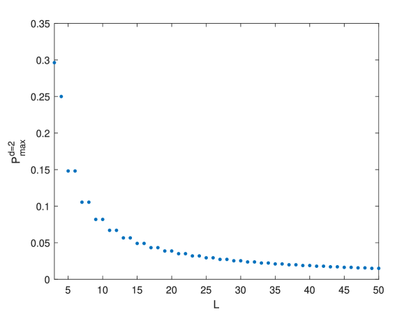
Figure 5: Optimisation over 2-state automata. The upper bounds (red) follow a pattern, where from $L=5$ on pairs of consecutive values coincide. Our bounds furthermore match the explicit automata found in [7] up to numerical precision, thus providing an exact bound and proving the optimality of the models found in  [7, 45]. The optimization was performed with MOSEK [2] and CVXPY [8]. Each solution was provided by the solver was tested to verify that linear and positivity constraints are satisfied up to numerical precision.

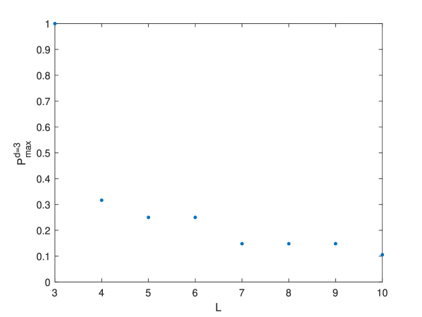
Figure 6: Optimisation over 3-state automata. Our method allows us also to optimize over 3-state automata, on which no previous analytical upper bound was derived. Again, we recover up to numerical precision the bound computed with the explicit model found in [7, 45], proving that our bound is exact and that the model previously found was optimal. The optimization was performed with SCS [33] and CVXPY [8]. Each solution provided by the solver was tested to verify that linear and positivity constraints are satisfied up to numerical precision.

In addition to the numerical values for $P^{\rm d}_{\rm max}$, we can also extract the value functions from our optimisations and use those to prove our bounds analytically. After deriving those value functions, we can further use them to find optimal automata for the problem at hand.

For extracting value functions, let us note first that from the numerical solutions the coefficients of the polynomials $V_{k}$ can be directly extracted, as these are optimisation variables of the problem. However, the value functions may not be unique and extracting polynomials with suitable (rational or integer) coefficients from the numerics is more challenging. Ways to further simplify these value functions are elaborated in Appendix B.2.

The method for optimising sequential models employed here allows us to derive upper bounds in terms of value functions, without treating the actual variables of the model – in this case the $\{p_{k}\}_{k}$ and $P$ – explicitly. A priori the solution does hence not tell us what the values of the optimal dynamical systems achieving the bounds may be, even if the bounds are tight. However, this can be remedied by first extracting the value functions from the optimisation and then running a second optimisation, this time fixing the value functions and optimising for the variables of the sequential model, here $\{p_{k}\}_{k}$ and $P$. More precisely, if we found an optimal upper bound $\nu^{\star}$, then all value function inequalities have to be tight and there is an optimal dynamical system that achieves the bound. Now if we can find a system that satisfies all inequalities with equality, then this will automatically be optimal. To find such a model, we can thus consider the optimisation problem

$$\max_{s_{k},\lambda,h_{k}}\ \ V_{1}(s_{1},\lambda)$$

such that $$V_{N}(s_{N},\lambda)=r_{N}(s_{N},h_{N},\lambda)$$

$$V_{k}(s_{k},\lambda)=r_{k}(s_{k},h_{k},\lambda)+V_{k+1}(f_{k}(s_{k},h_{k},\lambda),\lambda)$$ (26)

$$h_{k}\in H_{k}\ \forall k,\ s_{k}\in S_{k}\ \forall k,\ \lambda\in\Lambda$$

This is again a polynomial optimisation problem that can be solved with an SDP relaxation. In the following examples we use the solvemoment functionality of YALMIP [27] at level $4$ and the solver Mosek [2] to solve this. We find that in these cases the problem is feasible and we extract optimal automata.

• In the case $d=2$ and $L=3$ above, we obtain

  $$V_{1}(s_{1},\lambda)=(P(0,0|0)q_{1}(0)+P(0,0|1)q_{1}(1))P(b=1|0)+(P(1,0|0)q_{1}(0)+P(1,0|1)q_{1}(1))P(b=1|1),$$ (27)

  where $q_{k}(\sigma):=p_{k}(1,\sigma)$. Notice that in this case this is the natural optimisation problem one would also formulate directly to solve the problem at hand, however, for higher $L$ the decomposition into value functions differs. Now, using that the final reward is

  $$r_{2}=P(b=1|0)q_{2}(0)+P(b=1|1)q_{2}(1),$$ (28)

  and the state transition rules that translate to

  $$q_{2}(0)=P(0,0|0)q_{1}(0)+P(0,0|1)q_{1}(1),\quad q_{2}(1)=P(1,0|0)q_{1}(0)+P(1,0|1)q_{1}(1),$$ (29)

  we immediately see that $V_{1}(s_{1},\lambda)-r_{2}(s_{2}(s_{1}),\lambda)=0$. Furthermore, we can derive upper bounds on $V_{1}(s_{1}(s_{0}),\lambda)$, where we have from the state transition rules $q_{1}(0)=P(0,0|0)$ and $q_{1}(1)=P(1,0|0)$ (as the starting state is $q_{0}(1)=1$, $q_{0}(2)=0$) that

  $$V_{1}(s_{1}(s_{0}),\lambda)=(P(1,0|1)^{2}+P(2,0|1)P(1,0|2))P(b=1|1)+(P(1,0|1)P(2,0|1)+P(2,0|1)P(2,0|2))P(b=1|2).$$ (30)

  This gives a polynomial upper bound on the solution that indeed is upper bounded by $0.29630$, as a numerical maximisation of the value function over the $P$, $q_{k}$ confirms. The optimisation also shows that this maximum is achieved by an automaton with $P(0,0|0)=P(1,0|1)=\frac{1}{3}$, $P(1,0|0)=\frac{2}{3}$, $P(0,0|1)=0$, thus confirming this value as the optimal tight upper bound. This also coincides with the optimal automaton proposed in [7].

• For $d=2$ and $L=4$ we obtain the two value functions

  $$W_{2}(s_{2},\lambda) =V_{1}(s_{2},\lambda)$$

  $$W_{1}(s_{1},\lambda) =0.25(1+q_{1}(0)(q_{1}(0)-P(0,0|0))+q_{1}(1)(q_{1}(1)-P(1,0|0)))$$

  Now, we can see that 0.25 is an upper bound for $W_{1}(s_{1},\lambda)$, as the state update rules and $q_{0}(0)=1$, $q_{0}(1)=0$ in this case imply that $q_{1}(0)=P(0,0|0)$ and $q_{1}(1)=P(1,0|0)$. As a last relation  we have to check that

  $$W_{1}(s_{1},\lambda)-W_{2}(s_{2}(s_{1}),\lambda)\geq 0.$$ (31)

  A numerical optimisation confirms this polynomial inequality. Requiring that $W_{1}(s_{1},\lambda)=W_{2}(s_{2}(s_{1}),\lambda)$ while maximising $W_{1}(s_{1},\lambda)$ under the constraints on the $s_{1},s_{2}$ gives an optimal solution for the automaton of $P(1,0|0)=1$, $P(0,0|0)=0$ and $P(0,0|1)=\frac{1}{2}$, $P(1,0|1)=0$. This again coincides with the automaton from [7] for $L=4$.

Note that there are usually many different value functions that could solve the problem. Extracting value functions with few terms and integer or fractional coefficients from the optimisation problem, however, requires some tuning (see Appendix B.2). The process becomes more cumbersome as we increase the number of variables. We thus do not provide value functions for larger $L$ here. We remark that extracting valid value functions from the optimisation is, nevertheless, always possible.

IV.2 Entanglement detection in many-body systems: the multi-round GHZ game

To illustrate the performance of our SDP relaxations to solve entanglement certification problems in many-body systems, we consider an entanglement detection protocol inspired by the GHZ game, where the role of the memory is taken by a classical FSA. We thus call this protocol the multi-round GHZ game. Specifically, picture a protocol for entanglement verification where, in each of the first $N-1$ rounds, one of the following two measurements is performed with probability $\frac{1}{2}$:

$$M_{1}=\{M_{1|1}=|+\rangle\langle+|,\ M_{2|1}=|-\rangle\langle-|\}\ ,\quad M_{2}=\{M_{1|2}=|+i\rangle\langle+i|,\ M_{2|2}=|-i\rangle\langle-i|\},$$

where $|\pm\rangle=\frac{1}{\sqrt{2}}(|0\rangle\pm|1\rangle)$ and $|\pm i\rangle=\frac{1}{\sqrt{2}}(|0\rangle\pm i|1\rangle)$. This process is used to update the state of a four-state automaton that is initialised in state $t_{1}=1$ as displayed in Figure 7.

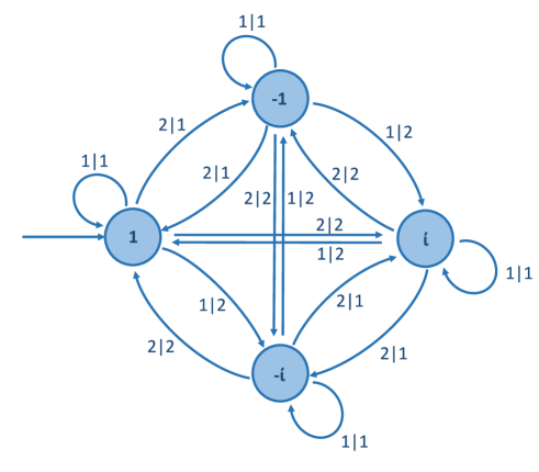
Figure 7: Memory update of the 4-state automaton in the GHZ-game. The transitions between states depend deterministically on $b$ and $y$, which are used to label the edges as $b|y$. In each round, this updates the automaton state $t\in\{1,-1,i,-i\}$.

In the final round, we choose measurement $1$ for states $t_{N}=\pm 1$ of the automaton and measurement $2$ for $t_{N}=\pm i$. The verification of an entangled state is considered successful if the outcome, $b_{N}$, of this additional measurement is $b_{N}=1$ for $t_{N}\in\{1,i\}$ or $b_{N}=2$ for $t_{N}\in\{-1,-i\}$, in which case we update $t_{N+1}$ to ’entangled’, otherwise ’separable’.

This protocol succeeds with probability 1 for a GHZ state of any dimension. Indeed, think of an $n$-partite GHZ-like state of the form

$$\frac{1}{\sqrt{2}}\left(|0\rangle^{\otimes n}+\alpha|1\rangle^{\otimes n}\right).$$ (32)

where $\alpha\in\{1,-1,i,-i\}$. Suppose that we measure one of the qubits state in the basis $\{|+\rangle,|-\rangle\}$ ($\{|i\rangle,|-i\rangle\}$), and obtain the result $|\pm\rangle$ ($|\pm i\rangle$). Then the final post-selected state is an $n-1$-partite state of the form (32), but this time with phase $\pm\alpha$ ($\mp i\alpha$).

Due to its transition matrix, the internal state of the automaton in Figure 7 keeps track of the phase of the GHZ-like state, as its qubits get sequentially measured, i.e., $t=\alpha$. The reward function simply verifies that the state of the last qubit corresponds to $\frac{1}{\sqrt{2}}(|0\rangle+\alpha|1\rangle)$.

The procedure introduced in Section III allows us to derive upper bounds on the maximum probability of success that is achievable with separable states $p_{\rm max}^{\rm sep}$. Our implementation relies on the representation of the pure state and measurements in terms of their Bloch vectors. We describe this in more detail in Appendix B.3. We display our bounds for different $N$ in Figure 8.

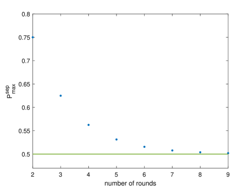
Figure 8: Upper bounds for the winning probability of the best separable states in the GHZ game. We observe that the winning probability (blue) drops quickly towards 0.5 (green line). The bounds are displayed up to $N=9$ for aesthetic reasons, in fact we checked that we can derive bounds up to $N=35$ with this method. With our asymptotic hierarchy (see Section VI.2) we further confirm an upper bound on the asymptotic value of $0.5004$ as $N\rightarrow\infty$.

Notice that the size of the optimisation problem allows us to reach round numbers as high as $N=35$. Details on the implementation (including precision issues and how to resolve them in this case) are presented in Appendix B.3.

V Asymptotic behaviour of sequential models

In some scenarios, the considered sequential problem admits a natural generalization to arbitrarily many rounds or time-steps $N$. In that case, we may also be interested in the asymptotic behaviour of the total reward as $N\rightarrow\infty$. However, as we shall see in the following (Section V.1), there are sequential models for which approximately computing the asymptotic maximum reward (or penalty) is an undecidable problem. Thus the best we can hope for are heuristics that work well in practice. In Section V.2 we introduce such heuristic methods and demonstrate in Section VI that these methods lead to useful bounds for the problems we considered in the finite regime in Sections IV.1 and IV.2.

V.1 Sequential models with uncomputable asymptotics

To see that there are sequential models for which the asymptotic maximum reward cannot be well-approximated, we rely on an intermediate result presented in [10], where specific probabilistic finite-state automata for which their asymptotic behaviour cannot be well-approximated were constructed.

Consider a finite-state automaton ${\cal A}$ with a (finite) state and input sets $\Sigma,X$, initial state $\sigma_{0}\in\Sigma$ and no outputs. The automaton is said to be freezable if there exists an input $x_{0}\in X$ that keeps the automaton in the same internal state. Call some subset $A\subset\Sigma$ the set of accepted states. Then we can consider how likely it is to bring the automaton’s state from $\sigma_{0}$ to some accepted state in $n$ time-steps by suitably choosing the input word $(x_{1},...,x_{n})\in X^{\times n}$. Define

$${\rm val}_{n}({\cal A})=\max_{\bar{x}\in X^{\times n}}\mbox{Prob}\left(\sigma_{n}\in A\right).$$ (33)

The automaton’s value ${\rm val}({\cal A})$ is defined as $\sup_{n}{\rm val}_{n}({\cal A})$. Note that, if ${\cal A}$ is freezable, then the function ${\rm val}_{n}({\cal A})$ is non-decreasing in $n$. In that case,

$${\rm val}({\cal A})=\lim_{n\to\infty}{\rm val}_{n}({\cal A}).$$ (34)

Given a freezable output-less automaton ${\cal A}$, consider the sequential model with $S_{k}$ being the set of probability distributions over $\Sigma$, ${H}_{k}=X$, $\Lambda=\emptyset$ and $s_{1}=\sigma_{0}$. The equation of motion is

$$P_{k+1}(\sigma^{\prime})=\sum_{\sigma}P_{k}(\sigma)P_{{\cal A}}(\sigma^{\prime}|\sigma,h),$$ (35)

where $P_{k+1}\in S_{k+1},P_{k}\in S_{k}$, and $P_{{\cal A}}$ denotes the automaton’s transition matrix.

In a sequential problem with $n$ rounds, we define the system’s reward as $r_{k}=0\ \forall\ k<n$, $r_{n}(s_{n})=\sum_{\sigma\in A}P_{n}(\sigma)$. From all the above, it is clear that the maximum total reward of the system corresponds to $\nu_{n}^{\star}:={\rm val}_{n}({\cal A})$. Hence, $\lim_{n\to\infty}\nu_{n}^{\star}={\rm val}_{n}({\cal A})$.

How difficult is to compute the asymptotic total reward for this kind of sequential models? The next result provides a very pessimistic answer.

Lemma 1 (Lemma 1 from [10]).

For any rational $\lambda\in(0,1]$, there exists a family ${\cal T}_{\lambda}$ of freezable probabilistic finite-state automata, with alphabet size $|X|=5$ and with $|\Sigma|=62$ states, such that, for all ${\cal A}\in T_{\lambda}$,

1. ${\rm val}({\cal A})\geq\lambda$ or ${\rm val}(({\cal A})\leq\frac{\lambda}{2}$.

2. it is undecidable which is the case.

Now, consider the class ${\cal C}$ of sequential problems for which the asymptotic value exists and is contained in $[0,1]$. This class contains the sequential problem of computing the value of any automaton in ${\cal T}_{1}$. It follows that there is no general algorithm to compute the asymptotic value of any sequential problem in ${\cal C}$ up to an error strictly smaller than $1/4$. Otherwise, one could use it to discriminate between the automata in ${\cal T}_{1}$ with value $1/2$ and those with value $1$, in contradiction with the lemma above.

V.2 Heuristic methods for computing upper bounds on the asymptotics of sequential models

Upper bounds on the asymptotic value of a sequential model as $N\rightarrow\infty$ can be achieved by deriving a function $\nu(N)$ that upper bounds the solution of the corresponding sequential problem of size $N$ for any $N$ and taking the limit. A way to achieve this is to encode, via functional constraints, recursion relations that define value functions for arbitrarily high $N$. For simplicity of presentation, let us consider a sequential model where $r_{k}=0$ for $k\not=N$ and $f_{k}$, $S_{k}$, $H_{k}$ are independent of $k$.

In the following, we show how to derive asymptotic bounds in case of convergence that is polynomial in $\frac{1}{N}$ as well as for exponential decay with $N$. Similar methods can also be used to bound the solution of the sequential problem even when the latter diverges, e.g., they can be used to prove that $\nu(N)\leq 4N^{3}$ (although, in this case, reducing the corresponding constraints to optimizations over functions of bounded variables might require some regularization trick (e.g.: $V_{k}\to V_{k}/k^{3}$).

V.2.1 Sequential models with polynomial speed of convergence in $\frac{1}{N}$

Let us assume that, for high $N$, $\nu(N)\approx\bar{\nu}+\frac{A}{N}$, and we wish to compute $A$. This problem might arise, for instance, when we wish to study the asymptotic type-I error of a quantum preparation game [48]. To simplify notation, we use negative indices $-j$ to denote $N-j$. Following the formulation (13), in order to obtain an upper bound on the solution of the sequential problem for size $N$, we need to find $\nu$, $\{V_{-j}(s,\lambda)\}_{j=0}^{N-1}$ such that

$$V_{0}(s,\lambda) \geq r(s,h,\lambda),$$ (36)

$$V_{-(j+1)}(s,\lambda) \geq V_{-j}(f(s,h,\lambda),h,\lambda),\ j=0,\ldots,N-1$$ (37)

$$\nu \geq V_{-(N-1)}(s_{1},\lambda).$$ (38)

Now, suppose that we manage to show that there exist functions $\{W_{-j}(s,\lambda)\}_{j=0}^{k}$, $W(\alpha,s,\lambda)$ such that

$$W_{0}(s,\lambda) \geq r(s,\lambda,h),$$ (39)

$$W_{-j}(s,\lambda) \geq W_{-(j-1)}(f(s,h,\lambda),\lambda),\ j=1,\ldots,k,$$ (40)

$$W\left(\frac{1}{k},s,\lambda\right) \geq W_{-k}(s,\lambda),$$ (41)

$$W\left(\frac{\alpha}{\alpha+1},s,\lambda\right) \geq W(\alpha,f(s,h,\lambda),\lambda),\ \forall\alpha\in\left[0,\frac{1}{k}\right]$$ (42)

Then, the functions

$$V_{-j}(s,\lambda):=\begin{cases}W_{-j}(s,\lambda)\quad&j=0,\ldots,k,\\ W\left(\frac{1}{j},s,\lambda\right)\quad&j=k+1,\ldots,N-1\end{cases}$$ (43)

satisfy the constraints (36), (37). Intuitively, in (41), (42), the variable $\alpha$ must be understood to represent $\frac{1}{j}$, in which case $\frac{\alpha}{\alpha+1}$ corresponds to $\frac{1}{j+1}$. The constraint (42) hence implies the recursion relation (37) for $j\geq k$, the case $j<k$ is already taken care of by (40). Note that the value of $\alpha$ is bounded; this is important if we wish to use polynomial optimization methods to enforce the inequality constraints (42), see Section VI.

Furthermore, if, for some real numbers $B,C,...$, the extra condition

$$\bar{\nu}+A\alpha+B\alpha^{2}+C\alpha^{3}+...\geq W\left(\alpha,s_{1},\lambda\right),\ \forall\alpha\in\left[0,\frac{1}{k}\right],$$ (44)

is satisfied, then, by eq. (38), the function $\bar{\nu}+A\alpha+B\alpha^{2}+C\alpha^{3}+...$ upper bounds the solution of the sequential problem. A heuristic to upper bound $\bar{\nu}^{\star}$ on the limit $\lim_{N\to\infty}\nu(N)$ thus consists in minimizing $\bar{\nu}$ under constraints (39), (40), (41), (42), (44).

The previous scheme is expected to work well in situations where, for high $N$, the optimal value functions $V_{0},...,V_{-(N-1)}$ of problem (13) satisfy $V_{-(N-1)}\approx\bar{V}+\frac{\tilde{V}}{N}$, for some functions $\bar{V},\tilde{V}$. That is, they work well as long as $\lim_{N\to\infty}V_{-(N-1)}$ exists. Experience with dynamical systems suggests, though, that even if the solution of the sequential problem tends to a given value $\bar{\nu}$, the sequence $(V_{-(N-1)})_{N}$ might asymptotically approach a limit cycle. In such a predicament, there would exist a natural number $\mathcal{C}$ (the period) and functions $\bar{V}^{0},...,\bar{V}^{\mathcal{C}-1}$ such that, for high enough $N$, $V_{-N}\approx\bar{V}^{R}$, with $R=N\mbox{ (mod }\mathcal{C})$.

This situation can also be accounted for by considering functions $\{W_{-j}(s,\lambda)\}_{j=0}^{k}$, $\{W^{j}(\alpha,s,\lambda)\}_{j=0}^{\mathcal{C}-1}$ such that

$$W_{0}(s,\lambda) \geq r(s,\lambda,h),$$

$$W_{-j}(s,\lambda) \geq W_{-(j-1)}(f(s,h,\lambda),\lambda),\ j=1,\ldots,k,$$

$$W^{0}\left(\frac{1}{k},s,\lambda\right) \geq W_{-k}(s,\lambda),$$

$$W^{1}\left(\frac{\alpha}{\alpha+1},s,\lambda\right) \geq W^{0}(\alpha,f(s,h,\lambda),\lambda),\ \forall\alpha\in\left[0,\frac{1}{k}\right],$$

$$\vdots$$

$$W^{\mathcal{C}-1}\left(\frac{\alpha}{\alpha+1},s,\lambda\right) \geq W^{\mathcal{C}-2}(\alpha,f(s,h,\lambda),\lambda),\ \forall\alpha\in\left[0,\frac{1}{k+\mathcal{C}-1}\right],$$

$$W^{0}\left(\frac{\alpha}{\alpha+1},s,\lambda\right) \geq W^{\mathcal{C}-1}(\alpha,f(s,h,\lambda),\lambda),\ \forall\alpha\in\left[0,\frac{1}{k+\mathcal{C}}\right].$$ (45)

V.2.2 Sequential models with exponential speed of convergence in $N$

Suppose that the speed of convergence of the sequential model is exponential, i.e., $\nu(N)\approx\bar{\nu}+A\gamma^{N}$, for $\gamma<1$. Assuming, for simplicity, that $\lim_{N\to\infty}V_{-(N-1)}$ exists, how could we estimate both $\bar{\nu}$ and $\gamma$?

One way to check that the postulated convergence rate holds is to verify the existence of functions $\{W_{-j}(s,\lambda)\}_{j=0}^{k}$, $W(\alpha,s,\lambda)$ such that

$$W_{0}(s,\lambda) \geq r(s,\lambda,h),$$

$$W_{-j}(s,\lambda) \geq W_{-(j-1)}(f(s,h,\lambda),\lambda),\ j=1,...,k,$$

$$W\left(\gamma^{k},s,\lambda\right) \geq W_{-k}(s,\lambda),$$

$$W(\gamma\alpha,s,\lambda) \geq W(\alpha,f(s,\lambda,h),\lambda),\ \forall\alpha\in\left[0,\gamma^{k}\right]$$ (46)

and (44) hold. The last line of the above equation is the induction constraint, wherein this time $\alpha$ is to be interpreted as $\gamma^{j}$. As before, we defined $\alpha$ in terms of $j$ such that the former quantity is bounded. To treat this problem within the formalism of convex optimization, one would try minimizing $\bar{\nu}$ for different values of $\gamma$. Each such minimization, if feasible, would result in an upper bound $\nu(N)$ on the solution of the sequential problem with $\nu(N)\approx\bar{\nu}+O(\gamma^{N})$.

V.3 Adaptation to finite numerical precision

In standard numerical optimizations, the computer outputs value functions that only satisfy the positivity constraints (36-44) approximately. More generally, conditions of the form $\bullet\geq 0$ are weakened to $\delta+\bullet\geq 0$, for some $1\gg\delta\geq 0$.

For small values of $\delta$, conditions (36-41) and (44) are not problematic, in the sense that a small infeasibility of any of these inequalities leads to a constant increase in the value function by that amount. This is why in the resolution of (13), we have so far not considered numerical precision issues explicitly. Indeed, let $\{\delta_{j}\}_{j=k+1}$ be such that

$$W_{0}(s,\lambda)+\delta_{0} \geq r(s,\lambda,h),$$

$$W_{-j}(s,\lambda)+\delta_{j} \geq W_{-(j-1)}(f(s,h,\lambda),\lambda),j=1,...,k,$$

$$W\left(\frac{1}{k},s,\lambda\right)+\delta_{k+1} \geq W_{-k}(s,\lambda),$$

$$\bar{\nu}+A\alpha+B\alpha^{2}+C\alpha^{2}+...+\delta_{\infty} \geq W\left(\alpha,s_{1},\lambda\right).$$ (47)

Then, the functions $\tilde{W}_{-j}:=W_{-j}+\sum_{i=0}^{j}\delta_{i}$, $\tilde{W}:=W+\sum_{i=0}^{k+1}\delta_{i}$ satisfy conditions (36-41). If, in addition, condition (42) is satisfied by the original functions, then

$$\bar{\nu}+\sum_{j=0}^{k+1}\delta_{k}+\delta_{\infty}$$ (48)

is a sound upper bound of the asymptotic value of the game.

However, precision issues become more problematic if the relation (42) is only satisfied approximately, i.e., if

$$W\left(\frac{\alpha}{\alpha+1},s,\lambda\right)+\hat{\delta}\geq W(\alpha,f(s,h,\lambda),\lambda).$$ (49)

In that case, for $N>k$, the optimal reward of the $N^{th}$ game round is upper bounded by

$$\bar{\nu}+\sum_{j=0}^{k+1}\delta_{k}+\delta_{\infty}+\hat{\delta}(N-k).$$ (50)

That is, the bound grows linearly with $N$. In that case, the asymptotic upper bounds $\bar{\nu}$ obtained numerically can only be considered valid for $N\ll O\left(\frac{1}{\hat{\delta}}\right)$.

VI Applications of asymptotic optimisation of time-ordered processes

In this section, we bound the asymptotic behaviour of the time-ordered processes that were treated at a finite regime in Sections IV.1 and IV.2 respectively, relying on the techniques from Section V. While the former is an example of polynomial speed of convergence in $\frac{1}{N}$, the latter illustrates the technique in the exponential case.

VI.1 Asymptotic behaviour of finite-state automata

The probability that a $2$-state automaton generates a one-tick sequence of length $L$ seems to converge to $0$ as $O\left(1/L\right)$. It can also be verified that this is the convergence rate of the optimal model found in [7]. In fact, this model gives the probability of the one-tick sequence

$$p(2k)=\frac{1}{k}\left(1-\frac{1}{k}\right)^{k-1}\approx\frac{1}{\mathbf{e}k},\text{ for }k\rightarrow\infty,$$ (51)

where $\mathbf{e}$ is the basis of natural logarithms, and $p(2k-1)=p(2k)$. This explicit example provides an upper bound on the converge rate for $\nu(L)$, i.e., $\nu(L)$ cannot converge to zero faster than $2/\mathbf{e}L$. Similarly to this model, the value $\nu(L)$ of the sequential game computed numerically satisfies $\nu(2k)=\nu(2k-1)$ from $k=2$ on-wards. This suggests to apply the relaxation (45), with $\mathcal{C}=2$.

Remember that $s_{k}:=(p_{k}(0),p_{k}(1))$, where $p_{k}(t)$ denotes the probability that the automaton has produced so far the outcome $0$ and is in state $t$, and $\lambda:=(P(\sigma^{\prime},0|\sigma):\sigma,\sigma^{\prime})$, the automaton’s transition matrix. We allow the discrete value functions $W_{-k}(s,\lambda)$ to be linear combinations of all monomials of the form $s^{a}\lambda^{b}$, with $a,b=0,1,2$. The continuous value functions $W^{1},W^{2}$ are linear combinations of the monomials $s^{a}\lambda^{b}\alpha^{c}$, with $a,b,c=0,1,2$. Positivity constraints such as the last line of (45) are mapped to a polynomial problem by multiplying the whole expression by $(1+\alpha)^{2}$.

To solve this problem, we used the SDP solver Mosek [2], in combination with YALMIP [27]. After $28$ iterations, Mosek returned the upper bound $0.0265$, together with the UNKNOWN message. The solution found by Mosek was, however, almost feasible, with parameters PFEAS$=4\times 10^{-7}$; DFEAS$=8.6\times 10^{-7}$ GFEAS$=7.5\times 10^{-11}$ and MU$=1.3\times 10^{-7}$. It is therefore reasonable to assume that the actual solution of the SDP, which for some reason Mosek could not find, is indeed close to $2\times 10^{-2}$. This figure is, indeed, greater than the conjectured null asymptotic value, but nonetheless a non-trivial upper bound thereof.

VI.2 Asymptotics of entanglement detection protocols

We observe that for small $N$, $p_{\rm max}^{\rm sep}$ behaves as

$$p_{\rm max}^{\rm sep}\approx\frac{1}{2}+\frac{1}{2^{N}}.$$ (52)

This value of $p^{\rm sep}$ can also be achieved, by preparing the separable state $|+\rangle^{\otimes N}$. For completeness, we illustrate this in Appendix C. This shows that our bounds from Figure 8 for the finite $N$ regime are tight (up to numerical precision).

The behaviour (52) also implies that we expect an asymptotic value of $\frac{1}{2}$. Implementing the procedure to bound the asymptotic behaviour from Section V.2.2, we were able to confirm an upper bound of $0.5004$, before running into precision problems using YALMIP and the solver Mosek. For the implementation we extended the one described in Appendix B.3 with the additional relations from Section V.2.2. Notice that a value of $\frac{1}{2}$ corresponds to randomly guessing whether the state is entangled and is thus achievable for any $N$ and a lower bound on $p_{\rm max}^{\rm sep}$. Note that gap between the success probability of $1$ for the GHZ-state and $\approx\frac{1}{2}$ for the worst-case separable state, approximately reaches the maximal possible value of such a gap of $\frac{1}{2}$. This illustrates that the multi-round GHZ game performs essentially optimally for the task of certifying the entanglement of a GHZ state.

VII Policies with guaranteed minimum reward

Let us complicate our sequential model a little bit, by adding a policy. The idea is that the parameters $x$ describing our policy also affects the system’s evolution, i.e.,

$$s_{k+1}=f_{k}(s_{k},h_{k},\lambda,x)$$ (53)

as well as the reward $r_{k}(s_{k},h_{k},\lambda,x)$ obtained in each time-step.

Ideally, we would like to find the policy $x$ that minimizes the maximum penalty. That is, we wish to solve the problem

$$\min_{x}\max_{h,\lambda}\ \sum_{k=1}^{N}r_{k}(s_{k},h_{k},\lambda,x),$$ (54)

under the assumption that eq. (53) holds and that we know the initial state $s_{1}$.

For fixed $x$, though, it might be intractable to compute the minimum expected reward. A more realistic and practical goal is thus to find a policy $x$ and a sufficiently small upper bound $\nu$ on its maximum reward (or penalty) $\nu^{\star}(x)$. This is the subject of the next section.

VII.1 Optimization over policies

For any $x$, let $\nu(x)$ denote an upper bound on $\nu^{\star}(x)$, obtained through some relaxation of problem (13). We propose to use standard gradient descent methods or some variant thereof, such as Adam [21], to identify a policy $x^{\star}$ with an acceptable guaranteed minimum reward $\nu(x^{\star})$.

More concretely, call $X$ the set of admissible policies, and assume that $X$ is convex. Starting from some guess $x^{(0)}$ on the optimal policy, and given some decreasing sequence of non-negative values $(\epsilon_{k})_{k}$, projected gradient descent works by applying the iterative equation

$$x^{(k+1)}=\pi_{X}\left({{x^{(k)}}}-\epsilon_{k}\nabla_{x}\nu(x^{(k)})\right),$$ (55)

where $\pi_{Z}(x)$ denotes the projection of vector $x$ in set $Z$, i.e., the vector $z\in Z$ closest to $x$ in Euclidean norm. For $k\gg 1$, we would expect policy $x^{(k)}$ to be close to minimal in terms of the guaranteed reward $\nu(x^{(k)})$.

The use of gradient methods requires estimating $\nabla_{x}\nu(\bar{x})$ for arbitrary policies $\bar{x}$. Considering that we have so far obtained bounds $\nu(x)$ (for fixed $x$) numerically from relaxations of (13), this task requires additional theoretical insight. The rest of this section is thus concerned with formulating an optimization problem to estimate the gradient of $\nu(x)$.

Suppose, for simplicity, that $x$ consists of just one real parameter, i.e., we wish to compute $\frac{d}{dx}\nu(\bar{x})$. Fix the policy to be $\bar{x}$, let $\delta x>0$, and let us consider problem (13). To arrive at a tractable problem, one normally considers a simplification of the following type:

$$\nu(\bar{x}):= \min_{V_{1},...,V_{N},\nu}\nu$$

such that $$V_{N}(s_{N},\lambda)\geq_{Q}r_{N}(s_{N},h,\lambda,\bar{x}),$$

$$V_{k}(s_{k},\lambda)\geq_{Q}r_{k}(s_{k},h,\lambda,\bar{x})+V_{k+1}(f_{k+1}(s_{k},h_{k},\lambda),\lambda),$$

$$\nu\geq_{Q}V_{1}(s_{1},\lambda).$$ (56)

Here the relation $a\geq_{Q}b$ signifies that the expression $a-b$, evaluated on some convex superset $Q$ of the set of probability distributions on the variables $\{s_{k},h_{k}\}_{k},\lambda$, is non-negative. In the polynomial problems considered in this article, this superset $Q$ is, in fact, dual to the positivstellensatz used to enforce the positivity constraints. In the case of Putinar’s positivstellensatz, $Q$ would correspond to the set of monomial averages $\{\langle z_{i_{1}}...z_{i_{N}}\rangle\}$ that, arranged in certain ways, define positive semidefinite matrices, see [25] for details.

Since $Q$ contains all probability distributions, $a\geq_{Q}b$ implies that $a\geq b$, and so the solution of (56) is a feasible point of (13) and hence an upper bound $\nu(\bar{x})$ on $\nu^{\star}(\bar{x})$. For the time being, we assume that the minimizer $V_{1},...,V_{N}$ of problem (56) is unique for policy $\bar{x}$. We will drop this assumption later.

Now, let us consider how problem (56) changes when we replace $\bar{x}$ by $\bar{x}+\delta x$. We assume not only that the solution satisfies $\nu(\bar{x}+\delta x)\approx\nu(\bar{x})+\mu\delta x$, but also that the optimal slack variables $V_{1},...,V_{N}$ also experience an infinitesimal change, i.e.,

$$V_{k}(s_{k},\lambda)\to V_{k}(s_{k},\lambda)+\hat{V}_{k}(s_{k},\lambda)\delta x.$$ (57)

That is, not only the solution is differentiable, but also the minimizer of the optimization problem.

Ignoring all terms of the form $o(\delta x)$ in (57), it is clear that $\nu+\mu\delta x$ is an upper bound on $\nu^{\star}(\bar{x}+\delta x)$ iff

$$V_{N}(s_{N},\lambda)+\hat{V}_{N}(s_{N},\lambda)\delta x\geq_{Q} \ r_{N}(s_{N},h,\lambda,\bar{x})+\frac{\partial}{\partial x}r_{N}(s_{N},h,\lambda,\bar{x})\delta x,$$ (58)

$$V_{k}(s_{k},\lambda)+\hat{V}_{k}(s_{k},\lambda)\delta x\geq_{Q} \ r_{k}(s_{k},h,\lambda,\bar{x})+\frac{\partial}{\partial x}r_{k}(s_{k},h,\lambda,\bar{x})\delta x+V_{k+1}(s_{k+1},\lambda)+\hat{V}_{k+1}(s_{k+1},\lambda)\delta x$$ (59)

$$\ +\delta x\sum_{\sigma}\frac{\partial V_{k+1}}{\partial s_{k+1}^{\sigma}}\frac{\partial f^{\sigma}_{k}(s_{k},h_{k},\lambda,x)}{\partial x}$$

$$\nu+\mu\delta x\geq_{Q} \ V_{1}(s_{1},\lambda)+\hat{V}_{1}(s_{1},\lambda)\delta x.$$ (60)

Here, the symbol $\sigma$ is used to denote the coordinates of $s_{k+1}$.

Our goal is now to turn this into an optimisation problem that allows us to find $\mu$. For this purpose it is useful to invoke the fact that the slack variables $\{V_{k}\}_{k}$ are optimal, i.e., they not only satisfy the conditions in problem (56), but all inequalities must be saturated. Namely, for each $k$, there exists $q\in Q$ such that

$$\left\langle V_{k}(s_{k},\lambda)-r_{k}(s_{k},h_{k},\lambda)-V_{k+1}(s_{k+1},\lambda)\right\rangle_{q}=0.$$ (61)

To proceed, we need the following lemma, which allows us to phrase the constraints (58)-(60) in terms of the quantities $\hat{V}_{k}$.

Lemma 2.

Let $a\geq_{Q}0$, and let the set $Q^{\prime}:=\{q:q\in Q,\langle a\rangle_{q}=0\}$ be non-empty. Then, $a+\hat{a}\delta x\geq_{Q}0$ for $\delta x\to 0^{+}$ iff $\hat{a}\geq_{Q^{\prime}}0$.

Proof.

$Q^{\prime}\subset Q$, so $a+\hat{a}\delta x\geq_{Q}0$ implies that $\hat{a}\geq_{Q^{\prime}}0$. To see the converse implication, note that, for $q\in Q\setminus Q^{\prime}$, $\langle a\rangle_{q}>0$, and therefore $\lim_{\delta x\to 0^{+}}\langle a+\hat{a}\delta x\rangle_{q}>0$. To determine if $\langle a+\hat{a}\delta x\rangle_{q}\geq 0$ for all $q\in Q$ in the limit $\delta x\to 0^{+}$, it is thus sufficient to check that the property holds for $q\in Q^{\prime}$, i.e., that $a\geq_{Q^{\prime}}0$. ∎

By duality, condition $\hat{a}\geq_{Q^{\prime}}0$ is equivalent to

$$\xi a+\hat{a}\geq_{Q}0,\mbox{ for some }\xi\in\mathbb{R}.$$ (62)

From the above equation and relations (61), it follows that (under the hypothesis that the minimizer $V$ is differentiable and unique at $\bar{x}$) the limit $D^{+}\nu(\bar{x})\equiv\lim_{\delta x\to 0^{+}}\frac{\nu(\bar{x}+\delta x)-\nu(\bar{x})}{\delta x}$ equals

$$\min_{\mu,\hat{V},\xi}\mu$$

such that $$\hat{V}_{N}(s_{k},\lambda)\geq_{Q}\frac{\partial}{\partial x}r_{N}(s_{N},h_{N},\lambda,\bar{x})+\xi_{N}\left(V_{N}(s_{k},\lambda)-r_{N}(s_{N},h_{N},\lambda,\bar{x})\right),$$

$$\hat{V}_{k}(s_{k},\lambda)\geq_{Q}\frac{\partial}{\partial x}r_{k}(s_{k},h,\lambda,\bar{x})+\hat{V}_{k+1}(s_{k+1},\lambda)+\sum_{\sigma}\frac{\partial V_{k+1}(s_{k+1},\lambda)}{\partial s_{k+1}^{\sigma}}\frac{\partial f^{\sigma}_{k}(s_{k},h_{k},\lambda,x)}{\partial x}+$$

$$\qquad\qquad\quad+\xi_{k}\left(V_{k}(s_{k},\lambda)-r_{k}(s_{k},h_{k},\lambda,\bar{x})-V_{k+1}(s_{k+1},\lambda)\right),$$

$$\mu\geq_{Q}\hat{V}_{1}(s_{1},\lambda)+\xi_{1}\left(\nu-V_{1}(s_{1},\lambda)\right).$$ (63)

If, in addition, the sets

$$Q^{\prime}_{k}:=\{q\in Q:q\left(V_{k}(s_{k},\lambda)-r_{k}(s_{k},h_{k},\lambda,\bar{x})-V_{k+1}(s_{k+1},\lambda)\right))=0\},k=1,...,N,$$

$$Q^{\prime}_{0}:=\{q\in Q:q\left(\nu-V_{1}(s_{1},\lambda)\right))=0\}$$ (64)

have each cardinality $1$, i.e., $Q_{k}^{\prime}=\{q_{k}\}$, the problem to solve becomes even simpler, namely:

$$\min_{\mu,\hat{V},\xi}\mu$$

such that $$q_{N}\left(\hat{V}_{N}(s_{k},\lambda)\right)=q_{N}\left(\frac{\partial}{\partial x}r_{N}(s_{N},h_{N},\lambda,\bar{x})\right),$$

$$q_{k}\left(\hat{V}_{k}(s_{k},\lambda)\right)=q_{k}\left(\frac{\partial}{\partial x}r_{k}(s_{k},h,\lambda,\bar{x})+\hat{V}_{k+1}(s_{k+1},\lambda)+\sum_{\sigma}\frac{\partial V_{k+1}(s_{k+1},\lambda)}{\partial s_{k+1}^{\sigma}}\frac{\partial f^{\sigma}_{k}(s_{k},h_{k},\lambda,x)}{\partial x}\right),$$

$$\mu=q_{0}\left(\hat{V}_{1}(s_{1},\lambda)\right).$$ (65)

The derivation of eq. (63) relies on the hypothesis that the optimal slack variables $V:=\{V_{k}\}_{k}$ for policy $x=\bar{x}$ are unique. Should not this be true, the procedure to compute $D^{+}\nu(\bar{x})$ requires solving a non-convex optimization problem. The reader can find it in Appendix D, together with a heuristic to tackle it.

Now, let us return to the case of a multi-variate policy $x$. If the gradient $\nabla_{x}\nu(\bar{x})$ exists, then its $i^{th}$ entry corresponds to the limit

$$\lim_{\delta x\to 0^{+}}\frac{\nu(\bar{x}+\delta x|i\rangle)-\nu(\bar{x})}{\delta x}.$$ (66)

Each of these entries can be computed, in turn, via the procedure sketched above. This requires solving an optimization problem of complexity comparable to that of computing $\nu(\bar{x})$. Moreover, each such optimization can be performed separately for each coordinate of $x$. Namely, the process of computing the gradient of $\nu(\bar{x})$ can be parallelized. This allows us, through (55), to optimize over policies consisting of arbitrarily many parameters, as long as we have enough resources to compute $\nu(\bar{x})$.

VIII Application: optimization of adaptive protocols for magic state detection

Magic states, i.e., states that cannot be expressed as convex combinations of stabilizer states, are a known resource for quantum computation: together with Clifford gates, they allow conducting universal quantum operations efficiently [4]. This raises the problem of certifying whether a given source of states is able to produce them [44].

In the qubit case, magic states are those that cannot be expressed as a convex combination of the eigenvectors of the three Pauli matrices. Equivalently, magic states are those whose Bloch vector $\vec{n}$ violates at least one of the inequalities:

$$\left\{\sum_{j=1}^{3}n_{j}a_{j}\leq 1:a_{1},a_{2},a_{3}\in\{-1,1\}\right\},$$ (67)

see Figure 9 for an illustration.

Figure 9: Qubit magic states. Represented in the Bloch sphere, magic states of a qubit are all those that lie outside the blue octahedron. In this section the goal is to certify whether a general state is magic or not.

We wish to devise an $N$-round adaptive measurement protocol that tells us whether a given source is preparing magic states. Namely, if the source can just produce non-magic states, we expect the protocol to declare the source ‘magic’ with low probability $e_{I}$ (the protocol’s type-I error). If, however, the source is actually preparing independent copies of any quantum state violating one of these inequalities by an amount greater than or equal to $\delta$, we wish the protocol to declare the source ‘non-magic’ with low probability $e_{II}$ (the protocol’s type-II error), see Figure 10.

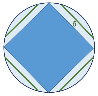
Figure 10: Illustration of magic state detection. We display a cut through the Bloch sphere showing non-magic (blue square) and magic states (region outside the square). The goal is to devise an $N$-round protocol that is able to reliably classify states into magic and non-magic ones, as long as the considered magic states are at least $\delta$ away from the non-magic ones. The protocol derived below, based on a $2$-state automaton, is valid in one of the regions outside the square of non-magic states.

To do so, we formulate the protocol as a time-independent preparation game [48]. That is, in every measurement round $k$, our knowledge of the state’s magic is encoded in the game’s configuration $t\in T$, with $|T|<\infty$. The state prepared by the source is then measured by means of the POVM with elements $(M_{t^{\prime}|t}:t^{\prime}\in T)\subset B({\mathbb{C}}^{2})^{\times|T|}$. The result $t^{\prime}$ of this measurement is the game’s new configuration. When we exceed the total number of measurement rounds $n$, we must guess, based on the current game configuration, whether the state source is magic or not. For simplicity, we declare the source to be magic if $t\in A\subset T$, with $|A|=\left\lfloor\frac{|T|}{2}\right\rfloor$. The initial state of the game, $t_{1}$, is chosen such that $t_{1}\not\in A$.

The game is thus defined by the POVMs $\{M_{t^{\prime}|t}:t^{\prime}\in T\}_{t}$. For computing $e_{I}$, we assume that the ‘dishonest’ player, who claims to produce magic states but does not, knows at every round the current game configuration. They can thus adapt their state preparation correspondingly to increase the type-I error. As explained in Section III.2, computing the maximum score of a preparation game under adaptive strategies can be cast as a sequential problem with $h_{k}:=(\rho_{k}(t):t\in T_{k})$. In this case, the $C$ set of feasible states is generated by convex combinations of $\{\psi_{i}\}_{i=1}^{6}$, the eigenvectors of the three Pauli matrices: linear maximizations over $C$ therefore correspond to maximizations over these six ‘vertices’. Putting it all together, we find that computing the game’s type-I error amounts to applying the recursion relation:

$$\mu_{N}(t) =\max_{i}\sum_{t^{\prime}\in A}\mbox{tr}(|\psi_{i}\rangle\!\langle\psi_{i}|M_{t^{\prime}|t}),$$

$$\mu_{k}(t) =\max_{i}\sum_{t^{\prime}}\mbox{tr}(|\psi_{i}\rangle\!\langle\psi_{i}|M_{t^{\prime}|t})\mu_{k+1}(t^{\prime}),$$

$$e_{I} =\mu_{1}(t_{1}).$$ (68)

Let us assume that all the maximizations above have a unique mazimizer, and call $i(k,t)$ the maximizer corresponding to the $k^{th}$ round and game configuration $t$. Then, the gradient of $e_{I}$ with respect to the POVM element $M_{\tau^{\prime}|\tau}$ satisfies the recursion relations:

$$\vec{\nabla}\mu_{N}(t) =\delta_{\tau,t}|\psi_{i(N,\tau)}\rangle\!\langle\psi_{i(N,\tau)}|,$$

$$\vec{\nabla}\mu_{k}(t) =\sum_{t^{\prime}}\mbox{tr}(|\psi_{i(k,t)}\rangle\!\langle\psi_{i(k,t)}|M_{t^{\prime}|t})\vec{\nabla}\mu_{k+1}(t^{\prime})+\delta_{\tau,t}\mu_{k+1}(\tau^{\prime})|\psi_{i(k,\tau)}\rangle\!\langle\psi_{i(k,\tau)}|,$$

$$\vec{\nabla}e_{I} =\vec{\nabla}\mu_{1}(t_{1}).$$ (69)

It can hence be computed efficiently in the number of measurement rounds.

Now, consider the computation of the type-II error under i.i.d. strategies, whose formulation as a sequential problem can be found in Section II.3. We first focus on the set ${\cal S}_{a}$ of qubit states with Bloch vector $\vec{n}$ satisfying $\sum_{j}a_{j}n_{j}\geq 1+\delta$, for some $a_{1},a_{2},a_{3}\in\{-1,1\}$. Applied to a source that always produces the same state $\rho\in{\cal S}$, the magic detection protocol can be modeled through a sequential model, with internal state $s_{k}$ at time $k$ given by the probability distribution over the game configurations $P_{k}(t)$ in round $k$, just before the measurement. The state $\rho\in{\cal S}$ prepared by the source is to be identified with the evolution parameters $\lambda$, as the equation of motion of the model is:

$$P_{k+1}(t^{\prime})=\sum_{t}\mbox{tr}(\rho M_{t^{\prime}|t})P_{k}(t).$$ (70)

To calculate the type-II error, we assign the model the rewards $r_{k}=0$, for $k=1,...,N-1$ and

$$r_{N}(P_{N},\rho)=\sum_{t}P_{N}(t)\sum_{t^{\prime}\in A}\mbox{tr}(\rho M_{t^{\prime}|t}).$$ (71)

We can thus compute an upper bound on $e_{II}({\cal S}_{a})$, the maximum type-II error achieved with states in class ${\cal S}_{a}$, via the SDP relaxation of eq. (13); and its gradient with respect to the POVM element $M_{t^{\prime}|t}$, via eq. (63) We assume that the solution of problem (13) is unique, so the techniques of Appendix D are not necessary.

Our original problem, though, is to compute the type-II error of all states violating at least one of the facets of the magic polytope by an amount $\geq\delta$. Thus we have that $e_{II}=\max_{a}e_{II}({\cal S}_{a})$. The gradient (or, more properly said, subgradient) of this function is $\vec{\nabla}e_{II}({\cal S}_{a^{\star}})$, where $a^{\star}$ is the argument of $\max_{a}e_{II}({\cal S}_{a})$.

Now we are ready to apply gradient descent to minimize the combined error $e_{I}+e_{II}$. We used the gradient method Adam [21], followed at each iteration by a projection onto the (convex) set of protocols $\{M_{t^{\prime}|t}:t^{\prime}\in T\}_{t\in T}$, with $M_{t^{\prime}|t}\geq 0,\forall t,t^{\prime}\in T,\sum_{t^{\prime}}M_{t^{\prime}|t}={\mathbb{I}},\forall t\in T$. For $|T|=2$, $n=6$, gradient descent converges to a value $e_{I}+e_{II}\approx 1$, probably an indication that one cannot detect all magic states with a $2$-state automaton. If, however, we restrict the problem to that of detecting those states that satisfy the inequality $\sum_{i}n_{i}\geq 1+\delta$, we arrive at the plot shown in Figure 11.

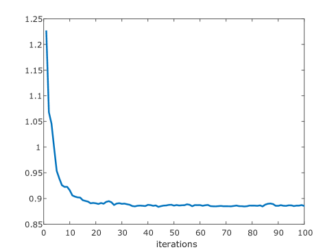
Figure 11: Upper bounds for $e_{I}+e_{II}$ as a function of the number of gradient iterations. Starting from a random preparation game, we used the Adam algorithm [21] to decrease the sum of the type-I and type-II errors of a magic-state detection protocol. For this computation, we set the algorithm’s learning rate to $0.01$.

As the reader can appreciate, after a few iterations, the algorithm successfully identifies a strategy with $e_{I}+e_{II}<1$. Beyond $50$ iterations, the objective value does not seem to decrease much further. This curve has to be understood as a proof-of-principle that gradient methods are useful to devise preparation games. Note that, for a general preparation game, the number of components of the gradient is $4|T|^{2}$. Optimizations over preparation games with high $|T|$ would thus benefit from the use of parallel processing to compute the whole gradient vector.

IX Conclusion

We have proposed a method to relax sequential problems involving a finite number of rounds. This method allows us to solve optimisation problems of sizes that were not tractable with previous convex optimisation techniques. Moreover, a variant of the method generates upper bounds on the solution of the problem in the asymptotic limit of infinitely many rounds.

We demonstrated the practical use of our methods by solving an open problem: namely, we computed the maximum probability for any finite state automaton of a certain fixed dimension to produce certain sequences, thus proving that the values conjectured in [7, 45] are optimal (up to numerical precision). We further illustrated how to turn such bounds into analytical results.

As we showed, the methods are also relevant in the context of certifying properties of quantum systems, especially in entanglement detection. Specifically, our method enables us to bound the misclassification error for separable states in multi-round schemes as well as in the asymptotic limit, which we illustrate by means of a GHZ-game inspired protocol, for which we also show that our bounds are tight.

Finally, we explained how to combine these methods with gradient descent techniques to optimize over sequential models with a certified maximum reward. This allowed the computer to generate an adaptive protocol for magic-state detection.

In some of our optimization problems, we found that otherwise successful SDP solvers, such as Mosek [2], failed in some cases to output a reliable result. The cause of this atypical behavior is unclear, and we lack a general solution for this issue. That said, the results from the numerical optimisation still allowed us to extract and confirm reliable bounds from the optimisations in most cases.

In two of the considered applications we found tight upper bounds on the quantities of interest. This may indicate that at least in reasonably simple cases our hierarchical method converges at relatively low levels of complexity. Finding conditions for convergence at such low levels is an interesting question that we leave open.

Quantum technologies are currently at the verge of building computing devices that can be used beyond purely academic purposes. These involve more than a few particles and thus the problem of certifying properties of systems of intermediate sizes is currently crucial. This is relevant not only from the perspective of a company building such devices but also from the perspective of a user who may want to test them independently. This progress is somewhat in tension with the state of research in certification, e.g. in entanglement theory, where methods are particularly abundant in the few copy regime (or asymptotically, when rates of generated resources are considered). Our analysis of the multi-round GHZ game is an example that illustrates that this type of analysis may bridge this gap. In particular, we expect that combining such an analysis with the optimization techniques introduced in the present work may allow to find certification protocols for large classes of many body systems. Our method is an alternative to the techniques based on shadow tomography [1, 20].

Our methods are furthermore able to certify systems beyond the linear regime that is employed when considering the usual types of witnesses for certifying systems, which from a mathematical viewpoint essentially distinguish convex sets by finding a separating hyperplane. As suggested in the example of magic states, our techniques beyond this regime also mean that we can analyse more general classes of systems simultaneously. Indeed, using a finite state automaton of large enough dimension, we expect to be able to detect any states that have at least a certain distance from the set of non-magic states. As optimisation methods improve, we expect such universal protocols to become more and more common as they are applicable also with minimal knowledge about the state of the system at hand.

Finally, many different problems encountered in quantum information theory have a sequential structure similar to the one analysed in this paper. Thus we expect that our methods will soon find applications beyond those studied in the present work. In this regard, it would be interesting to adapt our techniques to analyse quantum communication protocols. Another natural research line would be to extend our methods to model interactions with an evolving quantum system, rather than a (classical) finite state automaton.

Appendix A The Lasserre-Parrilo hierarchy and variants

The Lasserre-Parrilo method provides a complete hierarchy of sufficient conditions to certify that a polynomial is non-negative, if evaluated in a compact region defined by a finite number of polynomial inequalities [25, 34]. Given a number of polynomials $g_{1}(z),...,g_{u}(z),\tilde{g}_{1}(z),...,\tilde{g}_{v}(z)$, we define the region $Z\subset\mathbb{R}^{n}$ as

$$Z=\{z\in\mathbb{R}^{n}:g_{1}(z),...,g_{u}(z)\geq 0,\tilde{g}_{1}(z)=...=\tilde{g}_{v}(z)=0\}$$ (72)

Let $p(z)$ be a polynomial, and consider the problem of certifying that, for all $z\in Z$, $p(z)\geq 0$. A sufficient condition is that $p(z)$ can be expressed as

$$p(z)=\sum_{i}\tilde{g}_{i}(z)\tilde{f}_{i}(z)+\sum_{i}f^{i}(z)^{2}+\sum_{i,j}f^{i}_{j}(z)^{2}g_{j}(z),$$ (73)

where $\tilde{f}_{i}(z),f_{i}(z),f_{ij}(z)$ are polynomials on the vector variable $z$. The above is called a Sum of Squares (SOS) decomposition for polynomial $p(z)$. Deciding whether $p(z)$ admits a SOS with polynomials $\tilde{f}_{i}(z),f_{i}(z),f_{ij}(z)$ of bounded degree can be cast as a semidefinite program (SDP) [25]. Moreover, as shown in [25], as long as $Z$ is a bounded set and $p(z)$ is strictly positive in $Z$, such a decomposition always exists . A weaker criterion for positivity consists in demanding the existence of a decomposition

$$p(z)=\sum_{i}\tilde{g}_{i}(z)\tilde{f}_{i}(z)+\sum_{i}f^{i}(z)^{2}+\sum_{i,j}f^{i}_{j}(z)^{2}g_{j}(z)+\sum_{i}\sum_{j>k}f^{i}_{jk}(z)^{2}g_{j}(z)g_{k}(z)+\sum_{i}\sum_{j>k>l}f^{i}_{jk}(z)^{2}g_{j}(z)g_{k}(z)g_{l}(z)+...$$ (74)

If all terms in the decomposition have degree $n$ or less on its variables, we say that $p(z)\in SOS^{n}(g,\tilde{g})$.

We next sketch how to apply either hierarchy to tackle problem (13) in the main text. Let $(g^{k},\tilde{g}^{k})$ be the polynomials defining the sets $S_{k},S_{k+1},H_{k},\Lambda$, as well as the condition $s_{k+1}=f_{k}(s_{k},h_{k},\lambda)$. Take a sufficiently high natural number $n$ and consider the following SDP:

$$\nu^{n}:=\min_{V_{1},...,V_{N},\nu}\nu$$

such that $$V_{1},...,V_{N},\mbox{polynomials of degree $n$},$$

$$V_{N}(s_{N},\lambda)-r_{N}(s_{N},h,\lambda)\in SOS^{n}(g^{N},\tilde{g}^{N})$$

$$V_{k}(s_{k},\lambda)-r_{k}(s_{k},h,\lambda)-V_{k+1}(f_{k}(s_{k},h,\lambda),\lambda)\in SOS^{n}(g^{k},\tilde{g}^{k}),$$

$$\nu-V_{1}(s_{1},\lambda)\in SOS^{n}(g^{1},\tilde{g}^{1}).$$ (75)

From the discussion above, it follows that $\nu^{n}\geq\nu^{\star}$. Moreover, if $S_{k},H_{k},\Lambda$ are bounded, $\lim_{n\to\infty}\nu^{n}=\nu^{\star}$.

The same idea can be used to model constraints (44) and (46), by demanding the functions $\{W_{-j}\}_{j=0}^{k}$, $W$ to be polynomials of $\alpha,s,\lambda$. Because of the way we defined $\alpha$, this variable is bounded, and hence the Lasserre-Parrilo hierarchy is guaranteed to converge. Enforcing constraints of the form (42), where one of the polynomials is evaluated with $\frac{\alpha}{\alpha+1}$, can be dealt with by introducing a new variable $\beta$ representing $\frac{\alpha}{\alpha+1}$, together with the polynomial constraint $\beta(\alpha+1)=\alpha$. The latter, in turn, can be modeled though the conditions $\beta(\alpha+1)-\alpha\geq 0$, $\alpha-\beta(\alpha+1)\geq 0$.

In order to represent the conditions 73 and 74 in a SDP, we need to represent polynomials in a vector form. This is done, for instance, by fixing a basis of all monomials $\{m_{i}(z)\}_{i=1}^{N}$ up to the degree that is necessary to describe the polynomials in our problem. Let us denote this basis as ${\rm MB}_{\rm in}$. Each polynomial, then, is a linear combination of these monomials. This allows us to write the SOS condition in a SDP form, such as, e.g.,

$$\begin{split}\sum_{i}f^{i}(z)^{2}g(z)=\sum_{k,l}Z_{kl}m_{k}(z)m_{l}(z)g(z)\end{split}$$ (76)

for $Z$ an appropriately chosen positive-semidefinite matrix. Similarly, we have

$$\tilde{g}(z)\tilde{f}(z)=\sum_{i}\alpha_{i}g(z)m_{i}(z),$$ (77)

for some vector $\mathbf{\alpha}$. The results of these operations must, then, be written again in a vector form in terms of a new basis of monomial, which we denote as ${\rm MB}_{\rm out}$. The two bases, ${\rm MB}_{\rm in}$ and ${\rm MB}_{\rm out}$ allow us to represent all constraints as linear and positive-semidefinite constraints. See [25] for more details and the next sections for concrete implementations of this optimization problem.

Appendix B Implementation of optimisation of sequential models

B.1 Probability bounds for the one-tick sequence

In order to implement the optimization problem in Eq. (75), we need first to fix the relevant variables for describing our problem. To keep the notation lighter, we discuss the case $d=2$, the case $d=3$ can be easily understood as its generalization. To describe the states of the automaton we use the variables

$$s_{k}=(p_{k}(t_{k}=1,\sigma_{k+1}))_{\sigma},$$ (78)

with constraints $s_{k}^{0},s_{k}^{1}\geq 0$, $1-s_{k}^{0}-s_{k}^{1}\geq 0$, which gives two variable for each $k$. Notice that there is no need to describe the case $t_{k}=0$ as that would not contribute in the calculation of the probability of successfully outputing the one-tick sequence.

Similarly, for the transition parameters $\lambda$ one has just four variables: $\lambda:=(P(\sigma^{\prime},b=0|\sigma):\sigma,\sigma^{\prime}=0,1)$, since for the case $b=1$ we do not need to keep track of the internal state and the probability can be recovered by the normalization condition. They satisfy the constraints

$$P(\sigma^{\prime},b=0|\sigma)\geq 0,\mbox{ for all }\sigma,\sigma^{\prime}=0,1,$$

$$1-\sum_{\sigma^{\prime}}P(\sigma^{\prime},b=0|\sigma)\geq 0,\mbox{ for }\sigma=0,1.$$ (79)

Finally, there are the equality constraints that come from the the equation of motion

$$p_{k+1}(t_{k}=1,\sigma_{k+1})=\sum_{\sigma_{k}}p_{k}(t_{k-1}=1,\sigma_{k})P(\sigma_{k+1},0|\sigma_{k}),$$ (80)

for $k=1,...,L-1$. Finally, the initial state is fixed to be $s_{1}=(1,0)$.

This gives at each time step (except the initial and final one) four variables for the state $s_{k}^{0},s_{k}^{1},s_{k+1}^{0},s_{k+1}^{1}$ and four variables for the transition parameters $\{\lambda_{\sigma,\sigma^{\prime}}\}_{\sigma,\sigma^{\prime}=0,1}$. These are the variables on which the polynomials appearing in Eq. (72) are built.

To impose the problem’s constraints, we need the two bases of monomials ${\rm MB}_{\rm in}$ and ${\rm MB}_{\rm out}$ discussed in appendix A. These allow us to write the polynomials $g_{i},\tilde{g}_{i}$ appearing in the constraints in Eq. 72 as well as the polynomials in Eq. 73 and (possibly) Eq. 74, as vectors. For the specific calculations of the probability for the one-tick sequences, Figs. 5 and 6, it was sufficient to use Putinar’s positivstellensatz, i.e., Eq. 73. The input and output bases of monomials are chosen as follows.

• Construct three sets: monomials of degree two in the variables $(s_{k}^{0},s_{k}^{1})$, in the variables $(s_{k+1}^{0},s_{k+1}^{1})$ and in the variables $\{\lambda_{\sigma\sigma^{\prime}}\}_{\sigma\sigma^{\prime}}$.

• Combine these three sets together and add monomials of the form $s_{k}^{i}\lambda_{\sigma\sigma^{\prime}}$, for $\sigma,\sigma^{\prime},i=0,1$ and of the form $s_{k+1}^{i}\lambda_{\sigma\sigma^{\prime}}$ for $\sigma,\sigma^{\prime},i=0,1$. This operation concludes the construction of the input basis ${\rm MB}_{\rm in}$.

• Construct in a similar way two other bases, ${\rm MB}_{k}$ and ${\rm MB}_{k+1}$, defined as follows. ${\rm MB}_{k}$ is the union of monomials of degree two in the variables, respectively, $(s_{k}^{0},s_{k}^{1})$ and $\{\lambda_{\sigma\sigma^{\prime}}\}_{\sigma\sigma^{\prime}}$, together with monomials of the form $s_{k}^{i}\lambda_{\sigma\sigma^{\prime}}$, for $\sigma,\sigma^{\prime},i=0,1$. ${\rm MB}_{k+1}$ has the same construction with $s_{k}^{i}$ substituted by $s_{k+1}^{i}$. In other words, these bases are defined in the same way as ${\rm MB}_{\rm in}$, but this time excluding all monomials containing $s_{k+1}$ or containing $s_{k}$.

• The output basis is given by the tensor product of three copies of the input basis. In other word, each monomial of this list is a product of three monomials appearing in the input list. This concludes the construction of the output basis ${\rm MB}_{\rm out}$.

Once we have these bases, we want to implement the constraints

$$V_{k}(s_{k},\lambda)-V_{k+1}(s_{k+1},\lambda)\in SOS^{\ell}(g_{i},\tilde{g}_{i}),$$ (81)

where $SOS^{\ell}(g_{i},\tilde{g}_{i})$ denotes the fact that the SOS constraints are implemented up to a level $\ell$ which depends on the choice of the input (and possibly output) basis above. The function $V_{k}(s_{k},\lambda)$ is a polynomial given by a linear combination of monomials in the list ${\rm MB}_{k}$. Similarly, $V_{k+1}(s_{k+1},\lambda)$ is a linear combination of elements of ${\rm MB}_{k+1}$. The condition of belonging to $SOS^{\ell}(g_{i},\tilde{g}_{i})$ means that $V_{k}(s_{k},\lambda)-V_{k+1}(s_{k+1},\lambda)$ can be written in the form of Eq. 73 for properly chosen polynomials $\tilde{f}_{i},f_{i},f_{ij}$. In our implementation, $\tilde{f}_{i},f_{i},f_{ij}$ are convex combinations of monomials in the ${\rm MB}_{\rm in}$ basis. For the way in which ${\rm MB}_{\rm out}$ is chosen, all possible monomials arising from the product of $\tilde{f}_{i},f_{i},f_{ij}$ with $\tilde{g}_{i},g_{i}$ appear in ${\rm MB}_{\rm out}$.

For the case $d=2$, the SDP is run with CVXPY [8] and MOSEK [2] up to $L=50$. The values coincide with the explicit model found in [7] up to the fifth decimal digit. For the case $d=3$, the SDP is run with CVXPY [8] and SCS [33] up to $L=10$. The numerical solutions coincide with the optimal model found in [7] and the values explicitly reported in [45], up to the fourth decimal digit. For each explicit solutions provided by the solvers we verified that indeed the linear and positivity constraints are satisfied up to numerical precision.

B.2 Extracting value functions for the one-tick-sequences and finding optimal automata

In order to extract value functions that are suitable for further treatment, simplifications of the output of the polynomial optimisation (from B) is desirable. Here it is useful to impose any symmetries and additional knowledge regarding the structure of the problem at hand. This may allow us, for instance, to impose that certain monomials share the same coefficient and thus to reduce the number of independent variables.

In cases where there are redundant variables involved, we can further realise this by inspecting the value functions. If we had for instance chosen an implementation of the problem that additionally involves the variables $P(0,1|0)$ and $P(0,1|1)$, we could find value functions that don’t involve and of the monomials containing them. The other way around, we can check that we indeed need all variables used in the implementation of Appendix B, more precisely, while we could remove e.g. $P(0,0|1)$ or $P(1,0|1)$ in the $d=2$, $L=3$ case, these are needed for higher $L$.

As the numerical optimisation tends to assign non-zero values to all optimisation variables, it is further useful to simplify the value functions by eliminating irrelevant monomials, meaning setting their coefficients to zero. It turns out that this works well for the problem at hand when following a heuristic procedure by first computing the optimum $P^{\rm d*}_{\rm max}$ and then iterating the following two steps:

• Fix a threshold $\nu$ and set all coefficients of the $V_{k}$ smaller than $\nu$ to zero for the next optimisation. If there are no such coefficients, increase $\nu$.

• Solve the problem of optimising $P^{\rm d}_{\rm max}$ and check that the optimal value is still $P^{\rm d*}_{\rm max}$. If not, put coefficients back until recovering $P^{\rm d*}_{\rm max}$.

After this procedure the polynomials can then further be adjusted manually, e.g. by requiring that certain coefficients are equal.

B.3 Entanglement detection in the multi-round GHZ game

B.3.1 Implementation of a polynomial optimisation problem to bound the performance of separable states in the multi-round GHZ game

The multi-round GHZ state is conducted using a 4-state automaton that is updated by measuring a qubit state in each round. Due to normalisation, this means that we need polynomials in $3$ variables for the 4-state automaton, $\{p_{k}(t)\}_{t\in\{1,-1,i\}}$ , and $2$ variables for the Bloch vector of the state in each round, $n_{1},n_{2}$, where $n=(n_{1},n_{2},n_{3})$ denotes the Bloch vector of the state in round $k$, (except in the very last round, where we generate the reward as a function of $s_{N+1}$ in a way that updates this through multiplication with the success probability of the last measurement in each case. Due to the loss of normalisation the last step thus needs one additional polynomial variable).

The value functions are constructed following an adaptation of Schmüdgen’s positivstellensatz (74). The polynomials $V_{k}$ are taken to be of mixed degree $2$, i.e., terms of order up to $p_{k}(t)p_{k}(t^{\prime})n_{s}n_{s^{\prime}}$, $t,t^{\prime}\in\{1,-1,i\}$, $s,s^{\prime}\in\{1,2\}$. This means that for an inequality involving $V_{k}$ and $V_{k+1}$ we consider polynomials of degree up to 2 in each of $\{p_{k}(t)\}_{t\in\{1,-1,i\}}$, $\{p_{k+1}(t)\}_{t\in\{1,-1,i\}}$, $n_{1},\ n_{2}$, $n^{\prime}_{1},\ n^{\prime}_{2}$ (where $n=(n_{1},n_{2},n_{3})$ denotes the Bloch vector of the state in round $k$ and $n^{\prime}=(n^{\prime}_{1},n^{\prime}_{2},n^{\prime}_{3}$) is the Bloch vector in round $k+1$) This means that we consider monomials of the form $p_{k}(t)p_{k}(t^{\prime})p_{k+1}(t^{\prime\prime})p_{k+1}(t^{\prime\prime\prime})n_{s}n_{s^{\prime}}n^{\prime}_{s^{\prime\prime}}n^{\prime}_{s^{\prime\prime\prime}}$. The polynomials $g_{i}$ are here given by positivity of the probabilities of the automaton ($p_{k}(t=1)\geq 0,p_{k}(t=-1)\geq 0,p_{k}(t=i)\geq 0,1-p_{k}(t=1)-p_{k}(t=-1)-p_{k}(t=i)\geq 0$, and the same for $p_{k+1}$) as well as normalisation of the Bloch vectors of ($1-n_{1}^{2}-n_{2}^{2}\geq 0$ and $1-n_{1}^{\prime 2}-n_{2}^{\prime 2}\geq 0$). The equation of motion (5) for this example defines the $\tilde{g}_{i}$.

The equation of motion is in this case of degree $1$ in $p_{k}$, $p_{k+1}$, $\rho_{k}$, so that to exhaust the degree we have at our disposal we can multiply it with polynomials of degree $1$ in $p_{k}$, $p_{k+1}$, $\rho_{k}$ and degree $2$ in $\rho_{k+1}$. The squared polynomials multiplying the products $g=g_{j}g_{k}g_{l}...$ are chosen to be linear combination of at most degree $1$ in the variables that are not part of $g$.

B.3.2 Resolution of numerical problems in the optimisation of the multi-round GHZ game

We implemented the above problem using YALMIP [27] and the solver Mosek [2] for solving the semidefinite programs. To confirm that our results remain trustworthy for large $N$, we further extracted all value functions from the solution and then checked each inequality $V_{N}\geq r_{N}$, $V_{k}-V_{k+1}\ \forall k$, $\nu\geq V_{1}$ separately. For this purpose, we set up a constrained polynomial optimisation problem (constrained by positivity constraints and equation of motion) to maximise the violation of each inequality separately. As opposed to the case of the original optimisation we did not set up the semidefinite formulation manually but used the solvemoment functionality of YALMIP (setting level=$3$ except for k=30 where we used level=$2$) and Mosek for this step. The sum of the separate violations led to the error estimate for our results (see also Section V.3).

For $N=35$ we obtained a value of $0.5025$, where the upper bound was computed following the procedure (47) applied to the finite $N$ case with ${\nu}=0.5002$.

Appendix C Lower bound on the maximum winning probability in the multi-round GHZ game with separable states

The winning probability in the $N$-round GHZ game can be lower bounded by computing the score of any $N$-partite separable state. In the following we show that the optimal separable strategy consists in preparing the state $|+\rangle^{\otimes n}$, which indeed recovers our bounds (up to numerical precision).

For this state, the measurement outcome for measurement $1$ is $1$ in each round, while for measurement $2$, both outcomes occur with probability $\frac{1}{2}$. This means that the states of the automaton in round $k$ have probabilities ${\bf p_{k}}=(p_{k}(1),p_{k}(-1),p_{k}(i),p_{k}(-i))=(1/4+1/2^{n},1/4-1/2^{n},1/4,1/4)$, which is computed as ${\bf p_{k}}=M^{k-1}{\bf p_{1}}$, where ${\bf p_{1}}=(1,0,0,0)$ is the initial state of the sequential model and

$$M=\left(\begin{array}[]{rrrr}\frac{1}{2}&0&\frac{1}{4}&\frac{1}{4}\\ 0&\frac{1}{2}&\frac{1}{4}&\frac{1}{4}\\ \frac{1}{4}&\frac{1}{4}&\frac{1}{2}&0\\ \frac{1}{4}&\frac{1}{4}&0&\frac{1}{2}\\ \end{array}\right).$$

The final winning probability is $p^{\rm sep}(|+\rangle)=p_{N}(1)+\frac{1}{2}(p_{N}(i)+p_{N}(-i))$.

Appendix D Computing the gradient under non-uniqueness of the optimal value functions

The derivation of eq. (63) relies on the assumption that the optimal slack variables $V:=\{V_{k}\}_{k}$ for policy $x=\bar{x}$ are unique. In that case, it seemed natural to postulate that they are differentiable at $x=\bar{x}$, i.e., that the optimal slack variables of the perturbed problem, with policy $x=\bar{x}+\delta x$, should be of the form (57).

If there exists more than one minimizer for problem (56), though, then it is still natural to postulate that there exists at least one differentiable minimizer. However, there is no reason why the value of this minimizer should coincide with the value returned by the numerical solver. In other words, given a minimizer $V$ of (56), the optimization problem (63) in general returns an upper bound on $D^{+}\nu(\bar{x})$, rather than its exact value.

To tackle the possible non-uniqueness of the optimal slack variables $V$, consider, for fixed $\xi$, the following variant of problem (63):

$$\min_{\mu,V,\hat{V}}\mu$$

such that $$\hat{V}_{N}(s_{k},\lambda)\geq_{Q}\frac{\partial}{\partial x}r_{N}(s_{N},h_{N},\lambda,\bar{x})+\xi_{N}\left(V_{N}(s_{k},\lambda)-r_{N}(s_{N},h_{N},\lambda,\bar{x})\right),$$

$$\hat{V}_{k}(s_{k},\lambda)\geq_{Q}\frac{\partial}{\partial x}r_{k}(s_{k},h,\lambda,\bar{x})+\hat{V}_{k+1}(s_{k+1},\lambda)+\sum_{\sigma}\frac{\partial V_{k+1}(s_{k+1},\lambda)}{\partial s_{k+1}^{\sigma}}\frac{\partial f^{\sigma}_{k}(s_{k},h_{k},\lambda,x)}{\partial x}+$$

$$+\xi_{k}\left(V_{k}(s_{k},\lambda)-r_{k}(s_{k},h_{k},\lambda,\bar{x})-V_{k+1}(s_{k+1},\lambda)\right),$$

$$\mu\geq_{Q}\hat{V}_{1}(s_{1},\lambda)+\xi_{1}\left(\nu-V_{1}(s_{1},\lambda)\right),$$

$$V_{N}(s_{N},\lambda)\geq_{Q}r_{N}(s_{N},h,\lambda,\bar{x}),$$

$$V_{k}(s_{k},\lambda)\geq_{Q}r_{k}(s_{k},h,\lambda,\bar{x})+V_{k+1}(f_{k}(s_{k},h_{k},\lambda),\lambda),$$

$$\nu(\bar{x})\geq_{Q}V_{1}(s_{1},\lambda).$$ (82)

This problem optimizes, not just over $\hat{V}$, but also over the minimizers $V$ of problem (56).

A coordinate descent-based heuristic to compute the limit $D^{+}\nu(\bar{x})$ is thus the following: given a minimizer $V^{(j)}$ of the unperturbed problem, we solve problem (63), hence obtaining the slack variables $\xi^{(j)}$. Next, we solve problem (82) for $\xi=\xi^{(j)}$, obtaining the new unperturbed solution $V^{(j+1)}$. Starting from an initial solution of the unperturbed problem $V^{(0)}$, we hence generate a sequence of minimizers $V^{(1)},V^{(2)},...$ for problem (56). The corresponding sequence of solutions of problem (63), with $V=V^{(1)},V^{(2)},...$, is obviously decreasing, and, if the initial seed $V^{(0)}$ is close enough to the optimal solution, one would expect it to converge to $D^{+}\nu(\bar{x})$.

Since the estimation of $D^{+}\nu(\bar{x})$ requires solving a non-convex optimization problem, it is possible that the solution reached through coordinate descent is not optimal. A simple consistency check to verify that coordinate descent did not get stuck in a local minimum consists in computing the converse limit $D^{-}\nu(\bar{x}):=\lim_{\delta_{x}\to 0^{+}}\frac{\nu(\bar{x})-\nu(\bar{x}-\delta|i\rangle)}{\delta x}$ and see if both quantities coincide (they should, if $\nu(x)$ is differentiable in $x=\bar{x}$). It is not difficult to adapt the derivation of eqs. (63), (82) to estimate $D^{-}\nu(\bar{x})$ instead of $D^{+}\nu(\bar{x})$.