Label Assisted Autoencoder for Anomaly Detection in Power Generation Plants

Abstract

One of the critical factors that drive the economic development of a country and guarantee the sustainability of its industries is the constant availability of electricity. This is usually provided by the national electric grid. However, in developing countries where companies are emerging on a constant basis including telecommunication industries, those are still experiencing a non-stable electricity supply. Therefore, they have to rely on generators to guarantee their full functionality. Those generators depend on fuel to function and the rate of consumption gets usually high, if not monitored properly. Monitoring operation is usually carried out by a (non-expert) human. In some cases, this could be a tedious process, as some companies have reported an exaggerated high consumption rate. This work proposes a label assisted autoencoder for anomaly detection in the fuel consumed by power generating plants. In addition to the autoencoder model, we added a labelling assistance module that checks if an observation is labelled, the label is used to check the veracity of the corresponding anomaly classification given a threshold. A consensus is then reached on whether training should stop or whether the threshold should be updated or the training should continue with the search for hyper-parameters. Results show that the proposed model is highly efficient for reading anomalies with a detection accuracy of 97.20% which outperforms the existing model of 96.1% accuracy trained on the same dataset. In addition, the proposed model is able to classify the anomalies according to their degree of severity.

1 Introduction

About 3% of the world’s electrical energy is utilised by the information communication technology companies [1] and the telecommunication industry is one of the fastest growing industrial sectors among Agriculture, Banking, Infrastructure, and Oil and Gas. The number of telecommunication industries and the quest for expansion and growth has led to an increase in base stations across targeted countries to boost their network coverage and enhance the effective flow of communication. With the increase in the number of base stations, the issue of base station management needs to be addressed. Grid energy has been known to be the main source of power in developing countries such as those in Africa, and it is expected that these base stations located across different rural and urban areas will be powered by grid energy. However, electricity is quite unstable in most parts of these developing countries and this has forced base stations to look for a reliable alternative source of energy. These alternatives include photovoltaic panels (PV), wind turbines and diesel generators, but mostly generators due to a lack of space for the installation of PV or wind turbines [2]. The high cost of fuel and its transportation to supply stations located in rural areas has increased the operational cost of these companies. These generators are being refilled manually, thus creating room for irregular or unusual fuel consumption which might be caused by several reasons such as fuel theft, fuel leakages or poor maintenance of equipment. A study conducted in a base station in Cameroon has shown that the design of the base station building, room cooling systems such as air conditioners and careless handling of lights increase the rate of fuel consumption in the base station [3]. Espadafor et al. [4] also attested that generator performance can be affected by the age of the generator, the number of loads powered by the generator and improper maintenance.

In Cameroon, TeleInfra LTD is one such company whose objective is to manage base stations in various parts of the country. The services include maintenance of base stations and refuelling of generators. Like any other businesses relying on grid energy, the unstable power supply has resulted in high operating costs as companies have to find alternative sources of power supply to sustain the continuous operations of the business. The use of alternative sources such as solar panels, hybrid energy and generators has been implemented by TeleInfra for the sustainability of the business performance. Data on fuel consumed such as working hours of the generator, the quantity of fuel refuelled, the rate of consumption, generator maintenance, and total fuel consumed, are collected from base stations [5].

Although many strategies have been proposed to improve energy saving such as building a well-ventilated base station, the use of air conditioners as a cooling system and heat pipes to remove hot air from the base station [6]. However, detecting such irregularities is challenging especially when there are numerous base stations functioning at once. Anomaly detection in power generating plants is aimed at detecting such irregularities in the behaviour of the data provided. Although there are different algorithms for detecting anomalies, machine learning algorithms are the most used and popular for anomaly detection due to their ability for automation and their effectiveness in the context of deep learning, especially when involving large datasets. According to Goodfellow [7], deep learning is a variant of applied statistics with an increasing emphasis on using computers in estimating complex functions statistically, but a reduced emphasis on proving confidence intervals around these functions. Machine learning algorithms come in several variants. In supervised learning, models can make predictions on unlabelled data after they have been trained on labelled data whereas, in unsupervised learning, models can only make predictions on unlabelled data by learning similar features and patterns embedded in the datasets. In reinforcement learning, a goal is given and an agent undergoes training in an environment with the purpose of finding an optimal solution to accomplishing the goal.

Anomalies can be an indicator of areas that require attention, and detecting them has been quite popular among the research community. In the past, the research community has conducted several anomaly detections ranging from comprehensive to certain application domains with different machine learning algorithms. Mulongo et al. [5] worked on a similar area, four different supervised learning algorithms were used in their work for detecting an anomaly in a power generation plant. However, in real-life scenarios, abnormal behavioural patterns are very few compared to normal behaviour. For instance, in the same work of Mulongo et al. [5], labels were created by the authors based on certain criteria and only 35 per cent of the dataset turned out to be anomalous and the authors had to duplicate the data to balance between the two categories. These are key challenges in recognising anomalies with a supervised learning algorithm since they greatly rely on labelling and balance between normal and anomalous data patterns. The goal is to learn how efficiently a generating plant should behave so that observations that do not confine to the norm will be identified, and the required attention can be given. Our work investigates an alternative approach for anomaly detection in a power generation plant in an unsupervised manner based on the dataset used in Mulongo et al. [5]. The aim is to compare performance with the results obtained in Mulongo et al. [5]. The proposed unsupervised learning framework is built from a modifying and fine-tuning autoencoder which is free of the hassle of data labelling and balancing. An additional module is added to an autoencoder, the new module uses some labelled data to check if each of the observations is correctly classified and then one of the three steps below is activated:

• Update the threshold of the autoencoder which therefore increases the model overall accuracy to an acceptable level

• Update the interval of variation for numerical hyper-parameters, the best values of the hyper-parameters are then explored in the new search space

• Provide overall performance score

This paper is organised as follows: Section 2 explains anomaly detection and investigates related works for anomaly detection in power grid plants. Section 3 discusses autoencoders which replicate the input data through a compressed representation. This section also discusses the different evaluation metrics used in this work. Section 4 proposes the label assisted autoencoder and provides a detail discussion. The dataset and feature engineering are discussed in Section 5. Section 6 discusses the results and limitations, and Section 7 concludes the work.

2 Anomaly detection and related works

Anomalies also known as outliers often refer to instances or data samples that are significantly distanced from the main body of an examined data [8]. These distanced values often indicate a deviation from its established normal pattern which can sometimes be a measurement error or an indication of a data sample of a different population [9]. Outliers classification depends on the type and domain of the given data as well as the data analyst. Since many outliers are linked directly with abnormal behaviour, they are also referred to as deviants, anomalies, or abnormalities in the literature of statistics and data analysis [8]. According to [8], interpreting data is directly associated with the detection of anomalous samples. Demestichas et al. [9] suggested that it is essential to achieve the highest possible interpretability level to properly select the best anomaly detection method from different ranges of the relevant algorithm. There are two major categories of anomalies depending on the given dataset; multivariate and univariate [9]. Multivariate anomalies can be spotted in multi-dimensional data while univariate anomalies are spotted in a single-dimensional data. Besides the two categories of anomaly, there are other categories which depend on the distribution of the given data. Data samples that are considered anomalous when viewed against the entire dataset are point anomalies, while data samples that are considered anomalous with respect to meta-information related to the data sample are contextual anomalies [10]. In other words, contextual anomalies are classified based on local neighborhoods, while point anomalies are classified based on the overall dataset. Collective anomalies denote anomalous data collection samples which together are considered an anomalous pattern.

Fahim and Sillitti [11] provide two anomaly detection methods; statistical and machine learning methods. The statistical method uses various algorithms such as density-based, distance-based, parametric and statistical-based. However, Trinh et al. [12] noted that one of the major challenges that are encountered by this approach is the design of a suitable model that can accurately separate normal data from unusual data points. On the other hand, machine learning methods consist of both supervised and unsupervised learning algorithms in which dataset can either be labelled for supervised learning or unlabelled for unsupervised learning. Some advantages of this method are an enhancement of detection speeds and its ability to handle complexity with the less human intervention [13].

Many researchers have worked on different machine learning techniques for anomaly detection, but most of the current works applied artificial neural networks (ANNs) to classification tasks. The labelled data is used during the training stage, and then the learned model is able to correctly classify sample data never used during the training process. This technique is generally classified under supervised machine learning techniques. Such an example is trained in Mulongo et al [5] in which support vector machines (SVM [14]), K-Nearest Neighbours (KNN [15]), Logistic Regression (LR [16]), and MultiLayer Perceptron (MLP [17]) are used for anomaly detection associated with the fuel consumed dataset from an energy company. However, the energy sector is not the only place anomaly detection with supervised machine learning has been applied, others include fraud detection in credit card [18] attacks and anomaly detection in IoT sensors [19]. One of the main advantages of supervised learning techniques is the ability to handle high-dimensional datasets with high-performance [20]. However, there is a major problem with this technique. When dealing with real life data, the majority of them contains fewer anomalies data which is quite challenging and can cause the problem of an unbalanced dataset. This is an issue for supervised learning techniques since they greatly rely on labelled and balanced data. However, unsupervised learning techniques can be used to address this problem, for example, the autoencoder considers a specific kind of feed-forward neural network that can be applied in outlier-based anomaly detection rather than classification problems. Hawkins et al. [21] proposed an approach that involved autoencoder for outlier detection, however many researchers have investigated hybrid methods; e.g. [20] proposed an approach based on long short term memory (LSTM) autoencoder and One-class SVM (OC-SVM). The approach is used to detect anomalies based attacks in an unbalanced dataset. The idea is to use the LSTM-autoencoder to train a model to learn the pattern in the normal class (dataset without anomaly) so that-the model is able to replicate the input data at the output layer with a small reconstruction error. When there are anomalies in the data, the model fails to replicate the anomalous samples. This arises when the reconstruct error is very high.

Another unsupervised learning technique is the k-means, Zhang et al. [22], used the transformer model and the k-means clustering method for anomaly detection. The k-means was also used in the work of Munz et al. [23], to detect traffic anomalies, the main idea is to train data containing unlabelled records and separate them into clusters of normal and anomalous data.

3 Autoencoder and performance metrics

3.1 Autoencoder

An autoencoder is a neural network that is trained to attempt to copy its input to its output in an unsupervised manner. It consists of three parts: An Encoder part, a code and a decoder part. The encoder compresses the input data $\mathbf{X}$ defined in two dimensions as:

$$\mathbf{X} =\begin{pmatrix}\mathbf{X}_{1,1}&\mathbf{X}_{1,2}&\cdots&\mathbf{X}_{1,M}\\ \mathbf{X}_{2,1}&\mathbf{X}_{2,2}&\cdots&\mathbf{X}_{2,M}\\ \vdots&\vdots&\ddots&\vdots\\ \mathbf{X}_{N,1}&\mathbf{X}_{N,2}&\cdots&\mathbf{X}_{N,M}\end{pmatrix}\in\mathbb{R}^{N\times M}$$ (1)

where $\mathbf{X}_{:,i}\in\mathbb{R}^{N}$ is an observation with $N\in\mathbb{R}$ entries among the $M\in\mathbb{R}$ observations. The encoder compressed $\mathbf{X}$ to a lower-dimensional space $\mathbf{H}_{:,i}\in\mathbb{R}^{Q}$. The decoder produces a predicted output $\hat{\mathbf{X}}$,

$$\hat{\mathbf{X}} =\begin{pmatrix}\hat{\mathbf{X}}_{1,1}&\hat{\mathbf{X}}_{1,2}&\cdots&\hat{\mathbf{X}}_{1,M}\\ \hat{\mathbf{X}}_{2,1}&\hat{\mathbf{X}}_{2,2}&\cdots&\hat{\mathbf{X}}_{2,M}\\ \vdots&\vdots&\ddots&\vdots\\ \hat{\mathbf{X}}_{N,1}&\hat{\mathbf{X}}_{N,2}&\cdots&\hat{\mathbf{X}}_{N,M}\end{pmatrix}\in\mathbb{R}^{N\times M}$$ (2)

by reconstructing the original data from the compressed representation. It makes use of multiple layers and uses non-linear activation functions to learn the non-linear relationship embedded in the data. The goal is to make the reconstruction error as minimal as possible, which means finding the parameters that make the reconstruction $\hat{\mathbf{X}}$ as close as possible to the original input $\mathbf{X}$. Autoencoder can be applied to various tasks such as anomaly detection [20, 24], generative model [25, 26], clustering [27, 28], classification [29], recommendation systems [30] and dimensionality reduction [31, 32]. Figure 1 depicts a simple architecture of an autoencoder for which the detailed description is as follows:

Encoding: During the encoding process, assuming the input data $\mathbf{X}_{:,i}$ is a high dimensional vector that is mapped to a low dimensional vector $\mathbf{H}_{:,i}$ after filtering insignificant features. This is expressed mathematically as:

$$\mathbf{H}_{:,i}=f(\mathbf{X}_{:,i}),$$ (3)

where $f$ is a neural network that is trained with sets of activation functions weights and biases. Note that $f\in\mathbb{R}^{N}\rightarrow\mathbb{R}^{Q}$, where $Q$ is the number of compressed representations.

Decoding: During the decoding process, the compressed representation $\mathbf{H}_{:,i}$ of $\mathbf{X}_{:,i}$ is used to generate the output $\hat{\mathbf{X}}_{:,i}$ that maps back into the reconstruction of $\mathbf{X}_{:,i}$:

$$\hat{\mathbf{X}}_{:,i} =g(\mathbf{H}_{:,i})$$ (4)

$$=g\big{(}f(\mathbf{X}_{:,i})\big{)},$$ (5)

where $g$ is the decoding neural network with activation functions, weights, and biases that could be completely independent of the corresponding activation, weights, and biases of the encoding neural network. As discussed in [33, 34], the autoencoder involves the search for $f$ and $g$ which minimizes the average of the loss $\Delta_{\theta,\phi}$ between all the samples $\mathbf{X}_{:,i}$, added for example, to a $l_{2}$ weighted regularization term $a_{j}$:

$$[\hat{f},\hat{g}] =\operatorname*{arg\,min}_{f,g}\bigg{(}<\Delta_{\theta,\phi}\big{(}\mathbf{X}_{:,i},\hat{\mathbf{X}}_{:,i}\big{)}>+\lambda\sum_{j}a_{j}^{2}\bigg{)},$$ (6)

$$=\operatorname*{arg\,min}_{f,g}\bigg{(}<\Delta_{\theta,\phi}\big{(}\mathbf{X}_{:,i},g(f(\mathbf{X}_{:,i}))\big{)}>+\lambda\sum_{j}a_{j}^{2}\bigg{)},$$ (7)

where $<\cdot>$ is the average operator and $\lambda$ is the hyper-parameter that weights the regularization term, $a_{j}$. The higher the value of $\lambda$ the greater the capacity penalty. Note that $j$ runs across the hidden layers of the neural networks $f,g$. Finding the optimal neural networks $f$ and $g$ involves updating their respective learning parameters $\theta,\phi$ in each hidden layer of the neural networks so that the loss $\Delta_{\theta,\phi}$ is smaller than a given limit. In this work, the mean absolute loss:

$$<\Delta_{\theta,\phi}\big{(}\mathbf{X}_{:,i},\hat{\mathbf{X}}_{:,i}\big{)}>=\frac{1}{M}\sum_{i=1}^{M}\bigg{|}\mathbf{X}_{:,i}-\hat{\mathbf{X}}_{:,i}\bigg{|}$$ (8)

is used at the place of $<\cdot>$.

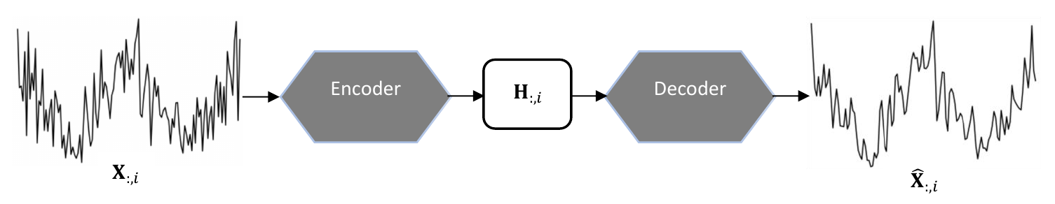
Figure 1: Simple architecture of an autoencoder (adapted from [35]).

3.2 Performance metrics

Performance metrics measure the ability of the overall quality of the model. A single performance measure is not enough to validate an autoencoder, therefore, different measures are performed and evaluated. The confusion matrix as shown in Table 1 generates more meaningful measures to find the detection accuracy, precision, recall, and F1 score. True Normal, $TN$ represents the number of observations in the normal class that are predicted as normal by the model (i.e. below the threshold). True Anomaly, $TA$ is the number of observations in the anomaly class that are predicted as an anomaly, and are above the threshold. False Normal, $FN$ is the number of anomalous observations that are below the threshold (i.e. predicted as normal classes). False Anomaly, $FA$ is the number of normal observations that are above the threshold (i.e. predicted as an anomaly).

Classification Class Distribution
	Actual Normal	Actual Anomaly
Predicted Normal	True Normal	False Normal
Predicted Anomaly	False Anomaly	True Anomaly

Table 1: Two class classification confusion matrix representation

The classification accuracy measures the general performance of the model by producing the ratio of true prediction (true normal and true anomaly) out of the total number of prediction:

$$Accuracy=\frac{TN+TA}{TA+TN+FA+FN}.$$ (9)

The Precision is the ratio of the true anomaly divided by the total number of observations above the threshold (i.e. number or anomalies predicted):

$$Precision=\frac{TA}{TA+FA}.$$ (10)

The False positive rate, $FPR$ refers to the ratio of the normal samples above the threshold to the actual number of anomalous samples:

$$FPR=\frac{FA}{FA+TN}.$$ (11)

True positive rate, $TPR$ also known as sensitivity or recall, is the ratio of the number of anomalous samples above the threshold to the actual number of samples in the anomaly class:

$$TPR=\frac{TA}{TA+FN}.$$ (12)

Specificity is a measure obtained from the outcome of the confusion matrix which gives the ratio of true anomaly to the total negative class in the sample:

$$\text{Specificity}=\frac{TN}{TN+FA}.$$ (13)

F-measure or $F_{1}$-score gives the harmonic mean between recall and precision of the classifier. High F-measure indicates a better performance of the classifier with no false alarm:

$$F\text{-measure}=2\left(\dfrac{\text{Precision}\times\text{Recall}}{\text{Precision}+\text{Recall}}\right).$$ (14)

4 Proposed label assisted autoencoder

4.1 The architecture of the proposed model

The encoder takes as input a high-dimensional input data here a fixed-size vector and reaches the latent space through mapping it to a a low-dimensional representational vector. The decoder reconstructs the input data from the reduced representation in the latent space. The final reconstruction error is used to set a threshold to detect anomalies. An additional computation block is added to check from a set of labelled data if the threshold is acceptable to satisfy the required precision. This is a kind of validation block that uses the threshold to decide if the threshold should be changed or if the autoencoder should be trained to further minimize the reconstruction loss. The entire architecture of the proposed assisted autoencoder is depicted in Figure 2 and a detailed description is provided below.

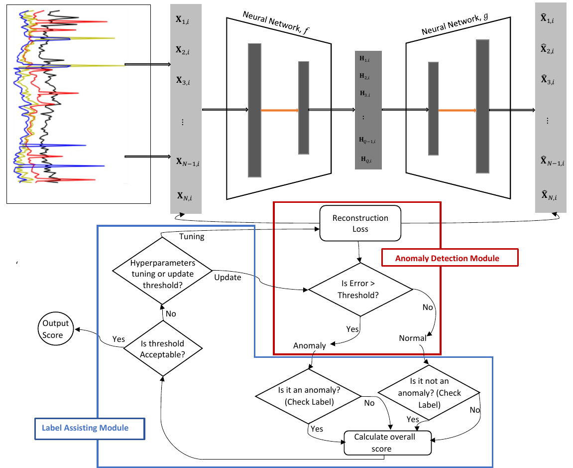
Figure 2: Overview of the proposed model. Each observation goes through the autoencoder for training, the reconstruction error is measured and then a threshold is used to make the decision whether the observation is an anomaly or not. The labelling assistance module then takes over to check if each of the observations is labelled, and then the label is used to check the veracity of the corresponding anomaly classification. A consensus is then reached whether training should stop or whether the threshold should be updated or the training should continue with the search for hyper-parameters.

1. The dataset is made up of observations and features which result in a 2-dimensional array of size $N\times M$, where $N$ and $M$ represent the number of features and the number of observations respectively. All features of each observation are collected and received as input in the algorithm called nodes.

2. The input data of size $N\times M$ is collected and reduced to a latent form of size $N\times Q$ where $Q<M$, while the $N\times Q$ set is fed into the decoder to produce a predicted output of size $N\times M$. Appendix Appendix A shows the parameters and the architecture of the deep neural networks trained in the encoder and decoder. The number of filters, size of filters and layers are displayed in the encoding and decoding phases.

3. After the decoding process, a reconstruction error is produced for each data point. The reconstruction error refers to the measure of how much the reconstructed input deviates from the original input. A threshold is set as a decision point to decide the acceptable amount of deviation, and the features of the observation that go beyond this threshold is classified as an anomaly. The observation that is below this threshold is a normal data without anomaly.

4. The label assisting module then takes over to verify if each of the observations is labelled, then the label is used to verify the veracity of the corresponding anomaly classification. The labelled observations are then checked and an agreement is reached if the threshold is satisfied to obtain the desired precision to detect anomalies, if not the threshold is updated or the model is further trained to find the best hyper-parameters for the given threshold.

To illustrate the above steps, an example of a scenario is described as follows. Assume the input data is $\mathbf{X}_{:,i}$ with $N$ features and their corresponding predictions given as:

$$\mathbf{X}_{:,i} =\mathbf{X}_{1,i},\mathbf{X}_{2,i},\mathbf{X}_{3,i},\cdots,\mathbf{X}_{N-1,i},\mathbf{X}_{N,i}$$ (15)

$$=(0.1,0.2,0.3,\cdots,0.4,0.5)$$ (16)

$$\hat{\mathbf{X}}_{:,i} =\hat{\mathbf{X}}_{1,i},\hat{\mathbf{X}}_{2,i},\hat{\mathbf{X}}_{3,i},\cdots,\hat{\mathbf{X}}_{N-1,i},\hat{\mathbf{X}}_{N,i}$$ (17)

$$=(0.6,0.21,0.32,\cdots,0.61,0.53)$$ (18)

The value of each of these features indicates the importance of the feature in the anomaly classification; e.g. the running time of a generator is more important than the generator capacity. The reconstruction loss for each feature is then calculated as in Equation 7:

$$L_{:,i} =|\mathbf{X}_{:,i}-\hat{\mathbf{X}}_{:,i}|$$ (19)

$$=(0.5,0.01,0.02,0.21,0.03).$$ (20)

Assume the maximum reconstruction loss is set to $0.2$, then the absolute error classifies the sample under the normal category while if a priority is given to the important feature, say $\mathbf{X}_{N-1,i}$ then the sample would be labelled as an anomaly since the reconstruction loss of $\mathbf{X}_{N-1,i}$ is $L_{N-1,i}=0.21$ which is beyond $0.2$. Figure 3 illustrates the reconstruction loss scenario adopted in this example.

4.2 Training and testing phases

Both the training and testing phases are equally important when it comes to the generalisation of the model. The dataset is divided into training and testing, depending on the proportion of choice, in our case, we used the ratio of 3:1 for training and testing respectively. The training phase is divided into two folds. Firstly, minimising the reconstruction error is the focus of the training for the reconstructed outputs to converge to the input samples. Secondly, the reconstruction error is calculated for each data point to find an optimal threshold for anomaly detection.

The training phase consists of normalizing the dataset so that all the features are reduced to a common scale without distorting the differences in the range of the values. In this work, the mathematical measure used to normalize the data is given by:

$$\mathbf{X}_{:,\mathrm{iscaled}}=\frac{\mathbf{X}_{:,i}-\mathbf{X}_{:,\mathrm{min}}}{\mathbf{X}_{:,\mathrm{max}}-\mathbf{X}_{:,\mathrm{min}}},$$ (21)

where $\mathbf{X}_{:,\mathrm{min}}$ and $\mathbf{X}_{:,\mathrm{max}}$ represent the data point with the minimum and maximum entries respectively. This is followed by dividing and separating the anomalous samples from the training set so that the algorithm learns to reconstruct the norms. Once the training is completed, a reconstruction loss between the input and output is calculated and a backpropagation strategy is applied to adjust the weights and parameters of the model. The testing phase checks the performance of the model on the unseen test data using the threshold obtained from the training phase. The whole process is described in Figure 3.

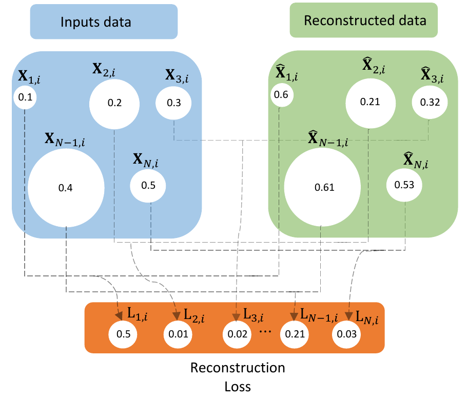
Figure 3: Computing reconstruction loss for $\mathbf{X}_{:,i}=(\mathbf{X}_{1,i},\mathbf{X}_{2,i},\mathbf{X}_{3,i},\cdots,\mathbf{X}_{N-1,i},\mathbf{X}_{N,i})$ using the predicted output $\hat{\mathbf{X}}_{:,i}=(\hat{\mathbf{X}}_{1,i},\hat{\mathbf{X}}_{2,i},\hat{\mathbf{X}}_{3,i},\cdots,\hat{\mathbf{X}}_{N-1,i},\hat{\mathbf{X}}_{N,i})$.

5 Datasets

5.1 Data description

The dataset used in this paper is gathered from a Telecom base station management company in Cameroon named TeleInfra and was subject to previous studies for anomaly detection in [5]. The dataset is collected over the period of one year, i.e. from September 2017 to September 2018. It consists of $6010$ observations from various base stations in 46 towns and villages (known as clusters) across Cameroon. These stations mainly rely on generators as the main supply of power. The dataset also consists of 17 variables which are defined in both numerical and categorical forms. A detailed description of each variable is shown in Table 2.

Feature Description
CONSUMPTION HIS	The total fuel consumed between a specific period of time before the next refuelling is done.
CONSUMPTION_RATE	The number of litres the generator consumes per hour.
Cluster	The cities where the generator sites are located
CURRENT HOUR METER GE1	The hour meter reading of the generator.
Site Name	Name of the site where each generator is located
EFFECTIVE_DATE_OF_VISIT	The date of meter reading, refuelling and recording
PREVIOUS_DATE_OF_VISIT	The previous date of visit
Months	The month when the reading was taken
NUMBER_OF_DAYS	The number of days before the next refuelling process.
GENERATOR_1_CAPACITY_(KVA)	The capacity of the generator
POWER TYPE	Type of power used in the power plant
PREVIOUS HOUR METER G1	The previous meter reading of the generator.
PREVIOUS_FUEL_QTE	The total quantity of fuel left inside the generator tank on the previous date of the visit.
QTE_FUEL_FOUND	The quantity of fuel found inside the generator tank before refuelling is done.
QTE_FUEL_ADDED	The quantity of fuel added to the generator during refuelling process.
TOTALE_QTE_LEFT	Quantity left in the generator after refuelling.
RUNNING_TIME	The total number of hours the generator worked before the next refuelling is done

Table 2: Description of the different features in the dataset.

Anomalies are observed in different features of the dataset and the observed anomalies are classified based on three indicators: (1) for a given time period if the generator running time is zero and the quantity of fuel consumed is not zero. (2) when the running time per day is more than 24 hours, and (3) when the daily consumed quantity of fuel is more than the maximum consumption a generator can consume. For a data sample to receive the anomaly tag 1, it has to demonstrate at least one of the three anomaly indicators listed, otherwise it is given the normal tag 0. A full workflow of the entire labelling process is illustrated in Figure 4. During the labelling process, output variables are assigned labels $0$ and $1$ representing the normal and anomaly classes respectively. For a single generator, Figure 5 illustrates the plot of the working hours per day, for example, all data samples above 24 h threshold show anomalies in the running time of one of the generators and these samples are assigned the label $1$ because it is known that one day only has 24 hours. The 6010 observations are curated to remove missing samples leaving 5902 observations with all information. Out of $5905$ observations, it is observed that $3832$ samples are labelled as normal and $2073$ samples as abnormal, resulting in 64.8% normal samples and 35.1% abnormalities in the entire dataset. Figure 6 shows all the clusters and their respective total fuel consumption including the degree of anomalies in the entire dataset.

5.2 Feature importance

Feature selection is performed by fitting the data using a random forest classifier with 16 features. Note that one could use any other method to find the most important feature. Since the relative importance of the most important feature is too high (100% as shown in Figure 7) compared to other features, any algorithm will predict the same feature as the most important. Figure 7 shows that the feature “Running time per day” has the greatest influence on the output and can be coined as the most important feature in the dataset. Even though it is followed by the “Daily consumption within a period” the huge difference between the “Running time per day” and the remaining features shows that priority should be given to the feature “Running time per day” when considering its reconstruction error for anomaly detection.

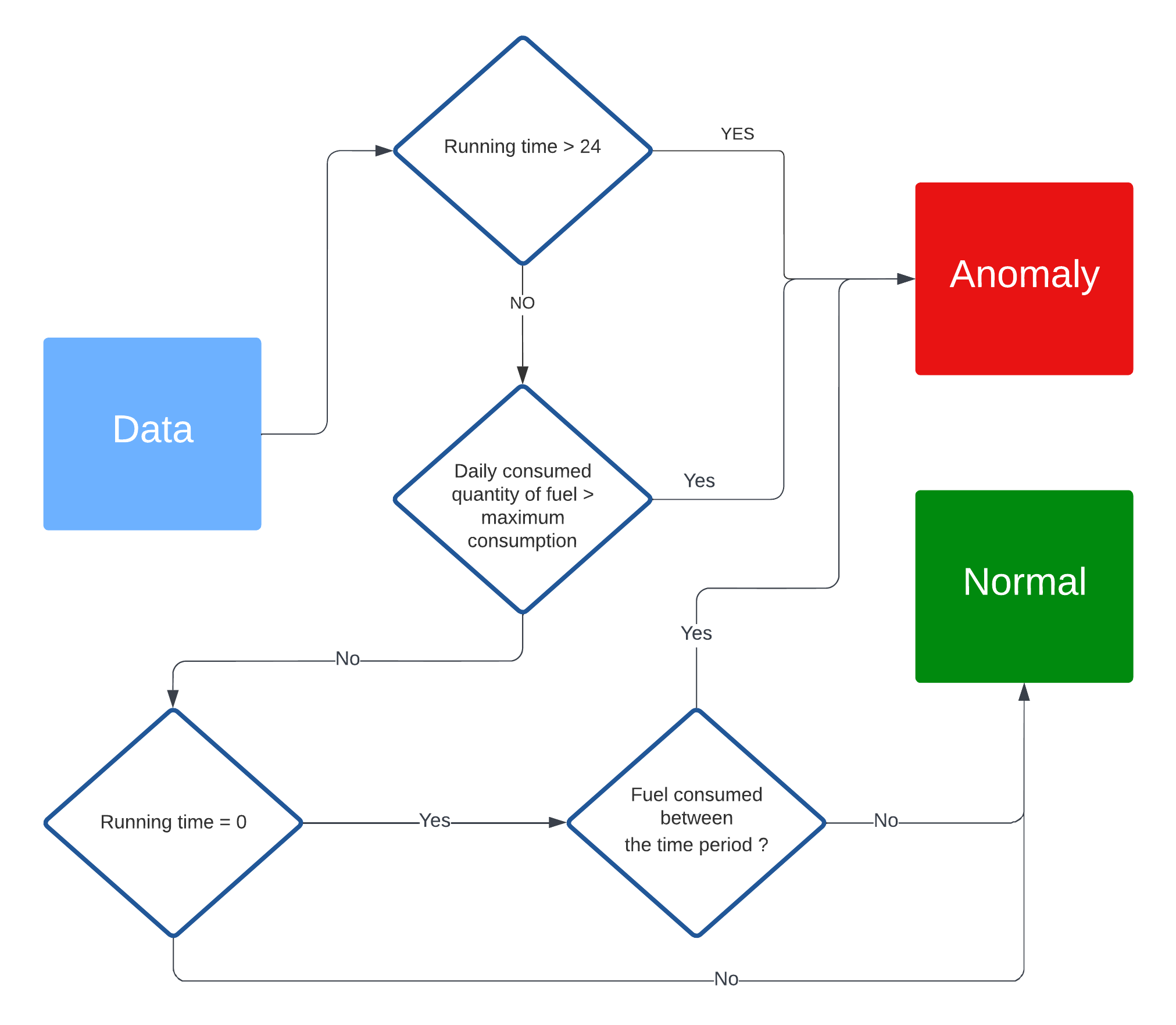
Figure 4: Flowchart showing how the labels are decided: For a data sample to receive the anomaly tag 1, it has to demonstrate at least one of the three anomaly indicators listed, otherwise it is given the normal tag 0.

5.3 Correlation

The correlation matrix is used to visualize the linear relationship between two variables. The values produced by the covariance matrix range from -1 to 1, where 1 indicates a strong positive linear relationship, -1 indicates a strong negative linear relationship and 0 indicates that there is no linear relationship between the variables. Figure 8 shows that the key variable “Running time per day” and the variable “Daily consumption within a period” has a strong positive correlation, which is reasonable since the daily quantity of fuel consumed by a generator is a function of the running time. A strong correlation is also observed between the three pairs of features; “Total quantity of fuel after refilling”, “Quantity of fuel found” and the “Previous quantity of fuel recorded”. However, the feature “Previous hour meter G1” has no significant correlation with any of the features.

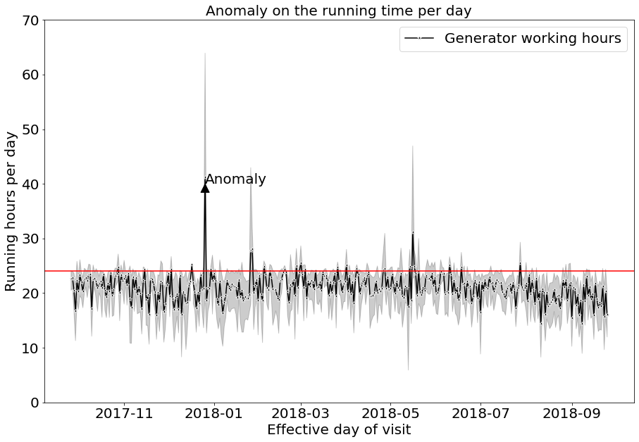
Figure 5: Observed anomaly in the number of working hours in a day for a single generator. For example, all data samples above 24 h threshold show anomalies in the running time of the generator and these samples are assigned the label $1$, because it is known that one day only has 24 hours.

6 Results

The results are observed from a number of different evaluation metrics.

6.1 Training

In order to assess the performance of our model during training, we set aside 10% of the training data as the validation set. The training and validation loss are seen in Figure 9 as it trends down different epochs. We observe that the validation loss is below the training loss. However, this can not influence the predicted accuracy with further hyper-parameter tuning since the difference between the two errors is negligible. The training loss accesses the error in the model during training. Finding the model’s appropriate threshold requires testing the model with the entire test dataset. The confusion matrix is used to get the model accuracy and True positive rate (TPR). They are plotted over a range of thresholds as seen in Figure 10(a) and the level at which they both attain an average maximum point is the best threshold for the model. As seen in Figure 10(a), the best threshold is 0.232 with an accuracy score of 0.962. However, if the sensitivity (TPR) or predicted anomaly is a priority for the organization without minding the cost they may secure while sorting out the False normal (predicted anomalies that are actually), the threshold could then be reduced to 0.231. This is the point where all anomalies are predicted (i.e. predicted anomalies are at 100%) with a higher false normal (FN) which has an effect on the overall model accuracy.

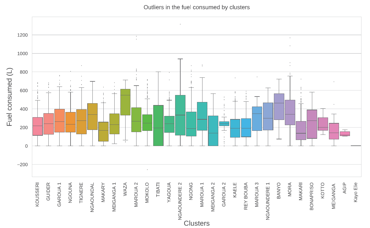
Figure 6: Fuel consumed per cluster showing the degree of anomalies in the dataset.

The threshold is also used to categorise these anomalies from mild to extreme using their reconstruction error. Figure 10(b) shows the reconstruction error. The samples with extreme threshold are prioritised when one seeks to find the reasons for the presence of anomalies.

6.2 Model performance

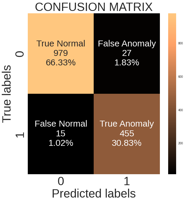
(a) Threshold = 0.232

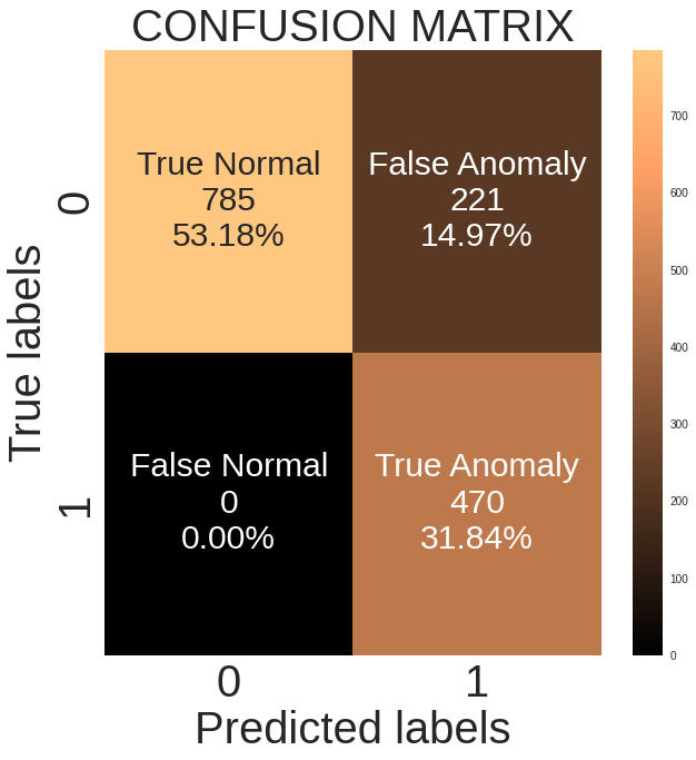
(b) Threshold = 0.231

Figure 11: Detection of results based on confusion matrix.

The total number of test samples is 1,476 with 1,006 normal samples and the remaining 470 are anomalous samples. Figure 11 illustrates the performance of the proposed model at different thresholds based on the confusion matrix. The proposed model is able to detect a total of 455 anomalous samples correctly out of the 470 samples with the anomaly label, this accounts for 96.8% (TPR) of the total anomaly samples. The model also detected a total number of 979 normal samples correctly out of 1006. The model incorrectly classified 15 normal samples as anomalies (FN) and 27 anomalies as normal samples (FA). These results show an accuracy of 97.15%, a precision of 94.40%, a recall of 96.81%, a specificity of 97.31% and a F1-score of 95.59%. Table 3 provides a summary of the performance metrics.

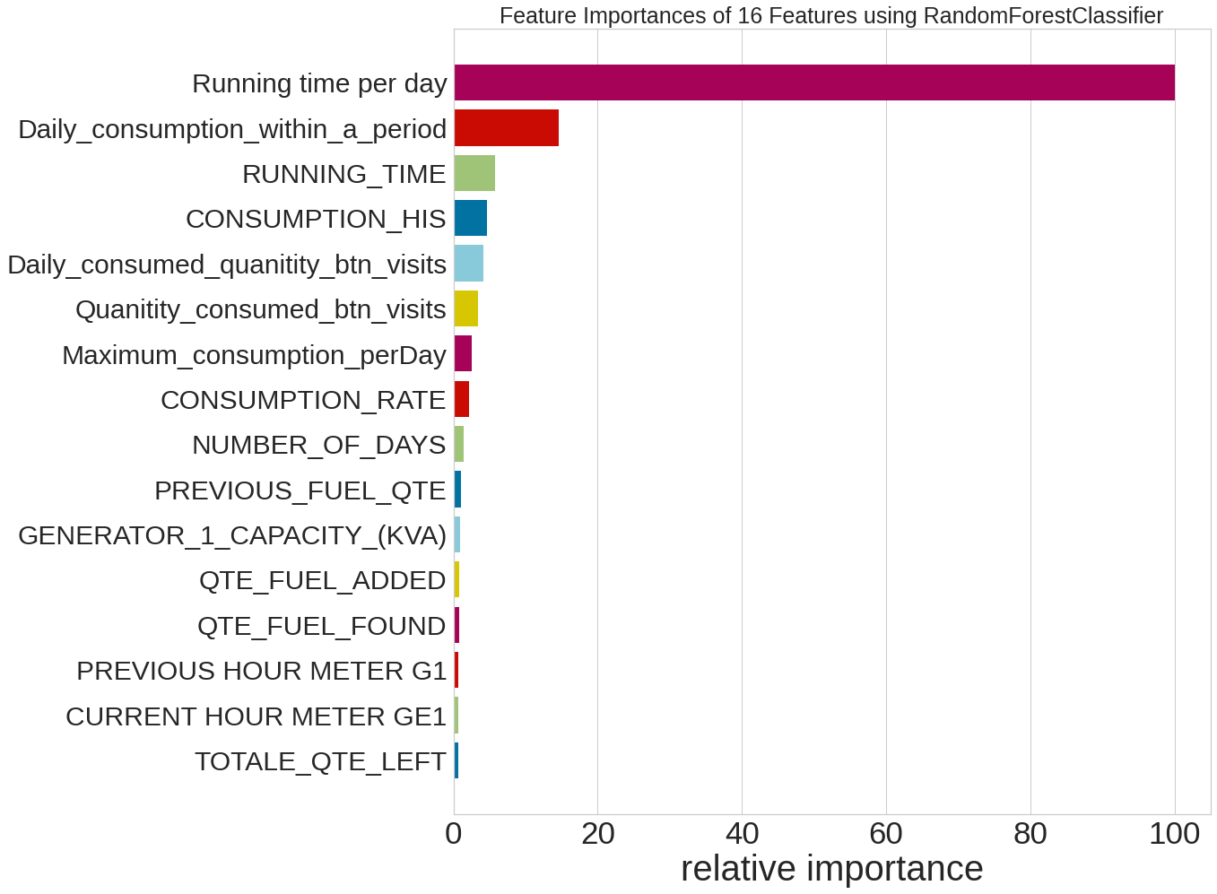
Figure 7: Feature importance for the 16 variables fitted using Random Forest Classifier. The feature “Running time per day” has the greatest influence on the output and can be coined as the most important feature in the dataset.

6.3 Comparison with other models using the same datatset

Table 4 shows the performance of the proposed model compared to that discussed in [5]. We used the latter paper to compare our work with because both are implemented using the same Teneifera dataset for anomaly detection. The proposed label assisted autoencoder has the best performance with an accuracy of 97.2% and a recall of 96.8%. The multi-layer perception proposed in [5] shows the most competitive performance with a higher F1-score, specificity and precision. However, the label assisted autoencoder is flexible since if we adjust the threshold, the recall will increase at the cost of specificity and overall accuracy.

6.4 Anomaly classification

The reconstruction error for each data sample differs from one another (as seen in Figure 10(b)) and provides an opportunity to classify these predicted anomalies according to their reconstruction error. In this work, 4 classes $A,B,C$, and $D$ are considered. Class $A$ represents anomalies that are slightly above the threshold, class $B$ represents anomalies that are above twice the threshold, class $C$ represents anomalies that are above four times the threshold, and class D represents anomalies that are above eight times the threshold. This implies that each class has twice a threshold compared to its predecessor. Table 5 shows the classes and their corresponding thresholds showing that 28.25% of the test dataset belongs to the anomaly category of class $A$, 2.03% belongs to class $B$, 0.20% belongs to class $C$ and 0.34% belongs to $D$.

6.5 Discussion

Feature importance has played an important role in this model, the feature “Running time per day” has the most significant importance of 100, and “Daily consumption within a period” coming in the second place with an important measure of 16, from this we gave priority to the reconstruction error of the “Running time per day”. To further justify our choice, the correlation matrix in Figure 8 shows a strong positive correlation of 0.74 between the two features. Using the reconstruction error of the key variable, we were able to train and compare the proposed model with the work in [5]. A recall score of 96.8% outperformed all the models proposed in [5] in detecting anomalies. Also, as shown in Table 3, our model shows a recall score of approximately 100% with a decrease in the overall accuracy of 85% when the threshold is decreased to 0.231.

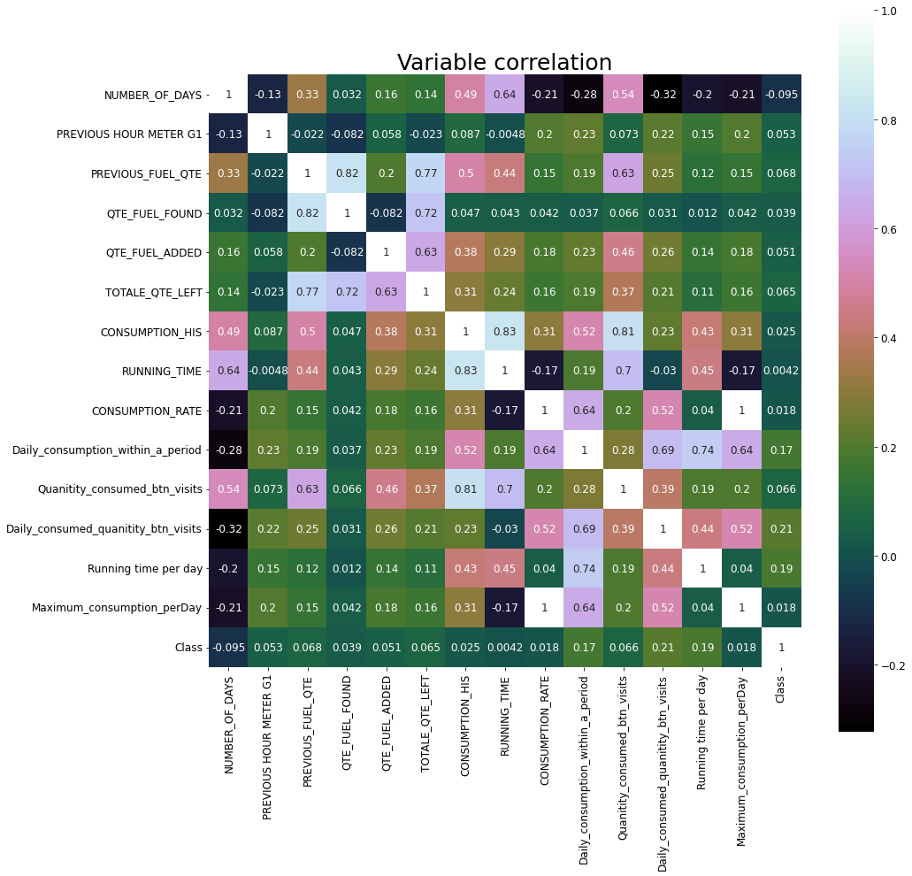
Figure 8: Correlation matrix of all numerical features. The “Running time per day” and “Daily consumption within a period” have a strong positive correlation, which is reasonable since the daily quantity of fuel consumed by a generator is a function of the running time.

7 Conclusion

Telecommunication industry is one of the dominant information communication technology industries that rely on a huge amount of electric power supply for their operations, and thus it is indispensable in their daily dealings. However, its availability in underdeveloped countries, particularly in Africa, has been a constant source of contention. Despite the industry’s rise through the creation of base stations, they have had to turn to alternative energy sources such as the use of gasoline or diesel with generators, and the use of solar power, to name a few.

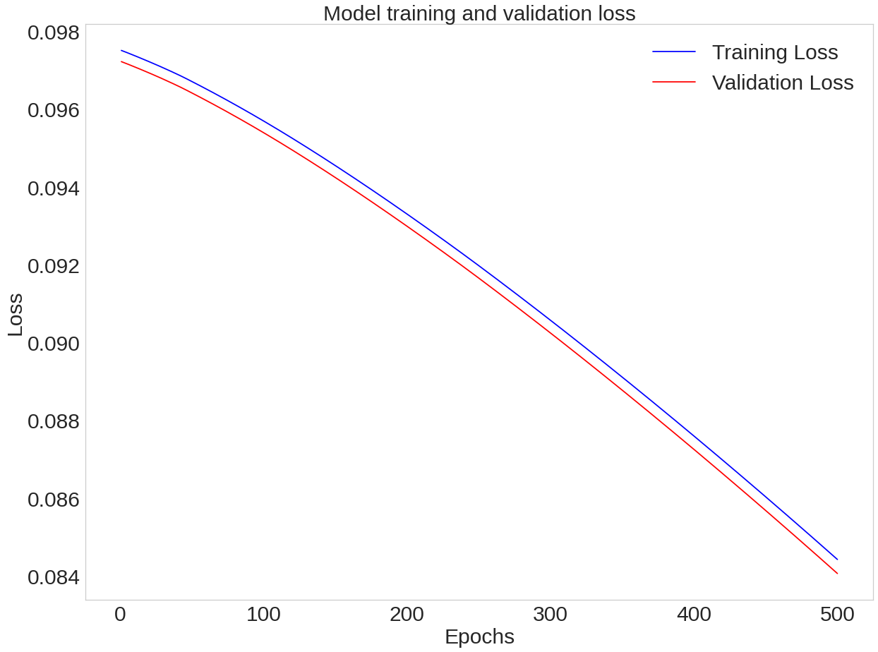
Figure 9: Training and validation loss as a function of the number of iterations. The mean absolute error is used to measure the loss.

TeleInfra telecommunication company established in Cameroon is one of such companies hooked on these challenges due to the state of power supply in the country. The telecommunication equipment that is fixed in different parts of the rural and urban areas in Cameroon requires an uninterrupted supply of electricity to achieve the goal of establishing strong and seamless communication channels in the country, however, the country’s electrical generation is mostly based on hydropower (73%), with perpetual power interruptions, particularly during the dry seasons when water levels are low [36]. The consequence of the diversification to alternative sources of power, particularly the usage of generators posed another challenge of irregularities or anomalies in fuel consumption at the base stations due to the observed high consumption rate in the power generation plants. TeleInfra telecommunication company is faced with the challenge of unaccounted high fuel consumption for their operations at the base stations. Since they solely depend on generating plants as their major source of power supply, they necessarily have to continually refill these generators and these are done manually. Such activities are known to have emanated in possible cases of pilferage of fuel due to the observed anomalies in fuel consumption. As a result, it is essential to investigate the likely factors contributing to the anomalies by collecting data on fuel consumption at each of the base stations for the purpose of minimizing the costs of operation.

We have proposed a label assisted autoencoder-based deep-learning technique for detecting anomalies in the fuel consumption datasets of the base station management company namely TeleInfra. In our proposed model, an autoencoder is used to generate an encoded representation of the input features and construct the output from the encoded representation to look like the input features of the series of decoders. The maximum reconstruction error from the trained model is obtained from the training set and it is set as a threshold for detecting anomalies on the test dataset. The anomaly detector identifies each data sample from the testing set as anomaly when they exceed the threshold assigned. Results showed that our proposed model is highly efficient for reading anomalies with a detection accuracy of 97.20% and outperforms existing supervised learning models. The proposed model is flexible and the threshold is adjustable according to the need of the user which can classify anomalies from severe to mild.

This work opens future research possibilities which could involve using different variations of autoencoders such as long short term memory autoencoders and memory-augmented autoencoders combined with our proposed label assisted unit. The latter does not require the feature importance analysis for selecting the best reconstruction error.

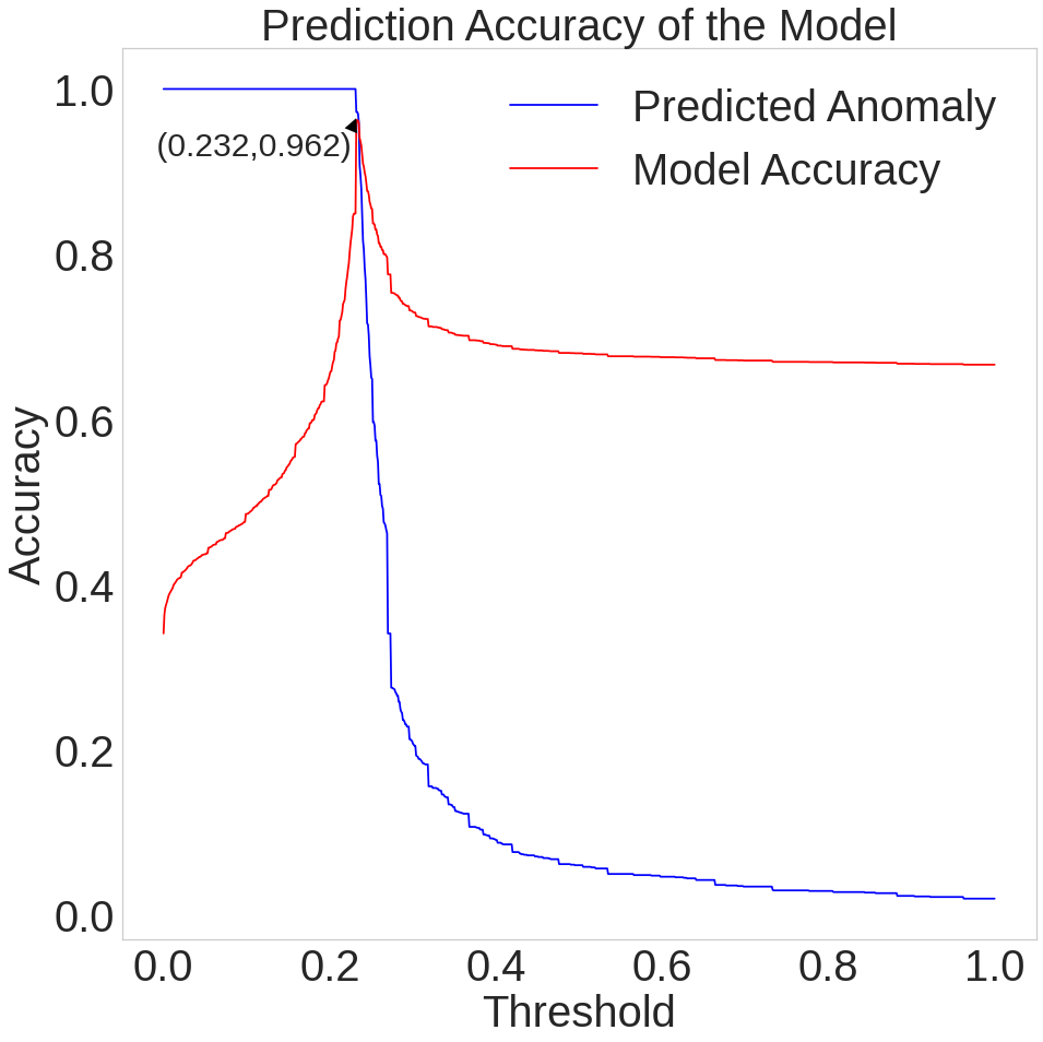
(a) Threshold detection

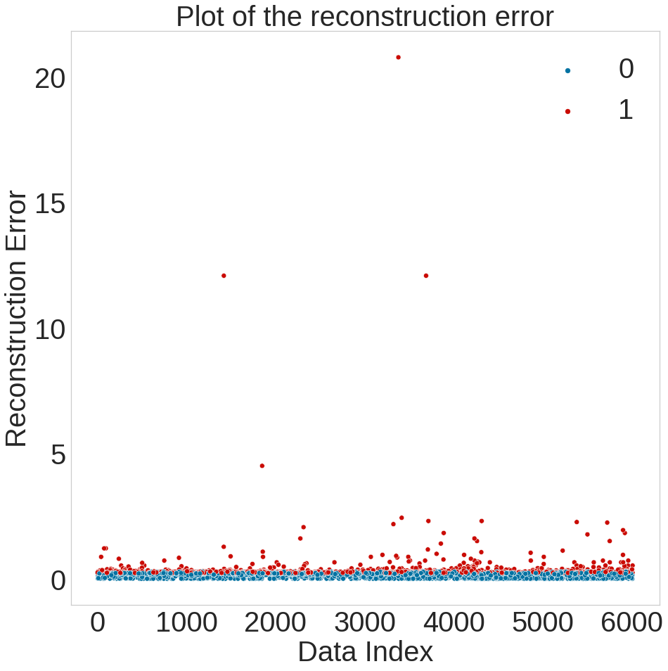
(b) Reconstruction Error

Figure 10: Threshold detection (10(a)) using the reconstruction error (10(b)). The threshold is used to categorise anomalies from mild to extreme using their reconstruction error.

Model performance
Threshold	Accuracy	F1-Measure	Recall	Precision	Specificity
0.232	0.972	0.956	0.968	0.944	0.973
0.231	0.850	0.810	1.00	0.680	0.780

Table 3: Evaluation performance.

Model performance
Paper	Techniques	Accuracy	F1-Score	Recall	Precision	Specificity
Mulongo et al. [5]	LR	0.708	0.811	0.709	0.943	0.699
	SVM	0.949	0.962	0.962	0962	0.925
	KNN	0.851	0.888	0.887	0.890	0.783
	MLP	0.961	0.971	0.954	0.988	0.976
Our Model	AE	0.972	0.956	0.968	0.944	0.973

Table 4: Comparison to similar models using the same dataset.

Categorizing Anomalies
Class	Threshold	Predicted Number of Samples	Percentage of Test Data
A	0.232	417	28.25%
B	0.464	30	2.03%
C	0.928	3	0.20%
D	1.856	5	0.34%

Table 5: Four categories of anomalies.

Disclosure Statement

We hereby state that no known competing financial interests or personal ties could have influenced the research presented in this study.

Appendix A

Architecture of deep neural networks trained in the encoder and decoder. The number of filters, size of filters and layers are displayed in the encoding and decoding phases.

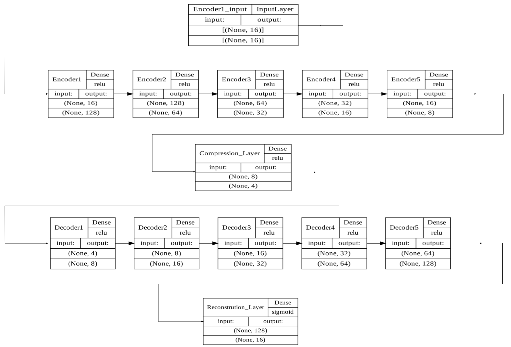
Figure 12: Architecture of the deep neural networks trained in the encoder and decoder.

References

- [1] I. Humar, X. Ge, L. Xiang, M. Jo, M. Chen, J. Zhang, Rethinking energy efficiency models of cellular networks with embodied energy, IEEE network 25 (2) (2011) 40–49.
- [2] J. Lorincz, I. Bule, Renewable energy sources for power supply of base station sites, International Journal of Business Data Communications and Networking (IJBDCN) 9 (3) (2013) 53–74.
- [3] A. Ayang, P.-S. Ngohe-Ekam, B. Videme, J. Temga, Power consumption: base stations of telecommunication in sahel zone of cameroon: typology based on the power consumption model and energy savings, Journal of Energy 2016.
- [4] F. J. Espadafor, J. B. Villanueva, M. T. García, Analysis of a diesel generator crankshaft failure, Engineering Failure Analysis 16 (7) (2009) 2333–2341.
- [5] J. Mulongo, M. Atemkeng, T. Ansah-Narh, R. Rockefeller, G. M. Nguegnang, M. A. Garuti, Anomaly detection in power generation plants using machine learning and neural networks, Applied Artificial Intelligence 34 (1) (2020) 64–79.
- [6] W. Jinggang, K. Ligai, D. Meixia, Z. Jin, G. Xiaoxia, Feasibility analysis using natural source cooling the idc plant, in: 2009 Chinese Control and Decision Conference, IEEE, 2009, pp. 2579–2584.
- [7] I. Goodfellow, Y. Bengio, A. Courville, Deep learning, MIT press, 2016.
- [8] C. C. Aggarwal, An introduction to outlier analysis, in: Outlier analysis, Springer, 2017, pp. 1–34.
- [9] K. Demestichas, T. Alexakis, N. Peppes, E. Adamopoulou, Comparative analysis of machine learning-based approaches for anomaly detection in vehicular data, Vehicles 3 (2) (2021) 171–186.
- [10] M. A. Hayes, M. A. Capretz, Contextual anomaly detection framework for big sensor data, Journal of Big Data 2 (1) (2015) 1–22.
- [11] M. Fahim, A. Sillitti, Anomaly detection, analysis and prediction techniques in iot environment: A systematic literature review, IEEE Access 7 (2019) 81664–81681.
- [12] H. D. Trinh, E. Zeydan, L. Giupponi, P. Dini, Detecting mobile traffic anomalies through physical control channel fingerprinting: A deep semi-supervised approach, IEEE Access 7 (2019) 152187–152201.
- [13] S. Omar, A. Ngadi, H. H. Jebur, Machine learning techniques for anomaly detection: an overview, International Journal of Computer Applications 79 (2).
- [14] S. Vishwanathan, M. N. Murty, Ssvm: a simple svm algorithm, in: Proceedings of the 2002 International Joint Conference on Neural Networks. IJCNN’02 (Cat. No. 02CH37290), Vol. 3, IEEE, 2002, pp. 2393–2398.
- [15] L. E. Peterson, K-nearest neighbor, Scholarpedia 4 (2) (2009) 1883.
- [16] T. G. Nick, K. M. Campbell, Logistic regression, Topics in biostatistics (2007) 273–301.
- [17] D. W. Ruck, S. K. Rogers, M. Kabrisky, Feature selection using a multilayer perceptron, Journal of Neural Network Computing 2 (2) (1990) 40–48.
- [18] S. Bhattacharyya, S. Jha, K. Tharakunnel, J. C. Westland, Data mining for credit card fraud: A comparative study, Decision Support Systems 50 (2011) 602–613.
- [19] M. Hasan, M. M. Islam, M. I. I. Zarif, M. Hashem, Attack and anomaly detection in iot sensors in iot sites using machine learning approaches, Internet of Things 7 (2019) 100059.
- [20] M. Said Elsayed, N.-A. Le-Khac, S. Dev, A. D. Jurcut, Network anomaly detection using lstm based autoencoder, in: Proceedings of the 16th ACM Symposium on QoS and Security for Wireless and Mobile Networks, 2020, pp. 37–45.
- [21] S. Hawkins, H. He, G. Williams, R. Baxter, Outlier detection using replicator neural networks, in: International Conference on Data Warehousing and Knowledge Discovery, Springer, 2002, pp. 170–180.
- [22] J. Zhang, H. Zhang, S. Ding, X. Zhang, Power consumption predicting and anomaly detection based on transformer and k-means, Frontiers in Energy Research (2021) 681.
- [23] G. Münz, S. Li, G. Carle, Traffic anomaly detection using k-means clustering, in: GI/ITG Workshop MMBnet, Vol. 7, 2007, p. 9.
- [24] C. Zhou, R. C. Paffenroth, Anomaly detection with robust deep autoencoders, in: Proceedings of the 23rd ACM SIGKDD international conference on knowledge discovery and data mining, 2017, pp. 665–674.
- [25] A. Mishra, S. Krishna Reddy, A. Mittal, H. A. Murthy, A generative model for zero shot learning using conditional variational autoencoders, in: Proceedings of the IEEE conference on computer vision and pattern recognition workshops, 2018, pp. 2188–2196.
- [26] G. R. Johnson, R. M. Donovan-Maiye, M. M. Maleckar, Generative modeling with conditional autoencoders: Building an integrated cell, arXiv preprint arXiv:1705.00092.
- [27] P. Ge, C.-X. Ren, D.-Q. Dai, J. Feng, S. Yan, Dual adversarial autoencoders for clustering, IEEE transactions on neural networks and learning systems 31 (4) (2019) 1417–1424.
- [28] X. Guo, X. Liu, E. Zhu, J. Yin, Deep clustering with convolutional autoencoders, in: International conference on neural information processing, Springer, 2017, pp. 373–382.
- [29] W. Luo, J. Li, J. Yang, W. Xu, J. Zhang, Convolutional sparse autoencoders for image classification, IEEE transactions on neural networks and learning systems 29 (7) (2017) 3289–3294.
- [30] D. Ferreira, S. Silva, A. Abelha, J. Machado, Recommendation system using autoencoders, Applied Sciences 10 (16) (2020) 5510.
- [31] M. Sakurada, T. Yairi, Anomaly detection using autoencoders with nonlinear dimensionality reduction, in: Proceedings of the MLSDA 2014 2nd workshop on machine learning for sensory data analysis, 2014, pp. 4–11.
- [32] W. Wang, Y. Huang, Y. Wang, L. Wang, Generalized autoencoder: A neural network framework for dimensionality reduction, in: Proceedings of the IEEE conference on computer vision and pattern recognition workshops, 2014, pp. 490–497.
- [33] U. Michelucci, An introduction to autoencoders, arXiv preprint arXiv:2201.03898.
- [34] Y. Wei, J. Jang-Jaccard, W. Xu, F. Sabrina, S. Camtepe, M. Boulic, Lstm-autoencoder based anomaly detection for indoor air quality time series data, IEEE Sensors Journal.
- [35] D. Bank, N. Koenigstein, R. Giryes, Autoencoders, arXiv preprint arXiv:2003.05991.
- [36] E. Muh, S. Amara, F. Tabet, Sustainable energy policies in cameroon: A holistic overview, Renewable and Sustainable Energy Reviews 82 (2018) 3420–3429. doi:https://doi.org/10.1016/j.rser.2017.10.049.