Flexible and Probabilistic Topology Tracking
with Partial Optimal Transport

Abstract

In this paper, we present a flexible and probabilistic framework for tracking topological features in time-varying scalar fields using merge trees and partial optimal transport. Merge trees are topological descriptors that record the evolution of connected components in the sublevel sets of scalar fields. We present a new technique for modeling and comparing merge trees using tools from partial optimal transport. In particular, we model a merge tree as a measure network, that is, a network equipped with a probability distribution, and define a notion of distance on the space of merge trees inspired by partial optimal transport. Such a distance offers a new and flexible perspective for encoding intrinsic and extrinsic information in the comparative measures of merge trees. More importantly, it gives rise to a partial matching between topological features in time-varying data, thus enabling flexible topology tracking for scientific simulations. Furthermore, such partial matching may be interpreted as probabilistic coupling between features at adjacent time steps, which gives rise to probabilistic tracking graphs. We derive a stability result for our distance and provide numerous experiments indicating the efficacy of distance in extracting meaningful feature tracks.

1 Introduction

Feature extraction and tracking for time-varying data play an important role in scientific visualization. Over the past two decades, topology-based techniques have been successfully applied to study the evolution of features of interest, which is at the core of many scientific applications, including combustion [1], climatology [2], and astronomy [3]. In particular, topology-based techniques utilize topological descriptors such as persistence diagrams and merge trees for feature extraction and tracking in scalar field data; see [4, 5] for surveys.

In this paper, we present a novel and flexible framework for tracking features (i.e., critical points) in time-varying scalar fields by combining merge trees with partial optimal transport. Merge trees are topological descriptors that record the evolution of connected components in the sublevel sets of scalar fields. Our contributions include:

• We present a new technique for modeling and comparing merge trees using tools from partial optimal transport. In particular, we model a merge tree as a measure network (that is, a network equipped with a probability distribution) and define a partial fused Gromov-Wasserstein distance between a pair of merge trees.

• We show that such a distance comes with good theoretical justifications and offers a new and flexible way to encode intrinsic and extrinsic information in the comparative measures of merge trees.

• Most importantly, we demonstrate via extensive experiments that such a distance gives rise to a partial matching between topological features in time-varying data, thus enabling flexible topology tracking for scientific simulations.

• Finally, the partial optimal transport provides a probabilistic coupling between features at adjacent time steps, which are then visualized by weighted tracks from probabilistic tracking graphs.

Furthermore, our implementation is open source, available at https://github.com/tdavislab/GWMT, including a video that demonstrates the probabilistic tracking graph.

Overview. After reviewing related work on partial optimal transport and topology-based feature tracking in Sect. 2, we review the technical background of merge trees, measure networks, and various distances used in (partial) optimal transport in Sect. 3. We then describe our feature-tracking framework in Sect. 4. In particular, we introduce a new distance – partial fused Gromov-Wasserstein distance – in Sect. 4.1 and describe its theoretical properties (Sect. 5). We demonstrate the utility of our framework with extensive experiments and comparisons with the state-of-the-art (Sect. 6). A direct consequence of our framework is that it enables richer representations of tracking graphs, referred to as probabilistic tracking graphs, for which we give a visual demonstration in Sect. 7.

2 Related Work

Optimal transport and Gromov-Wasserstein distance. This paper builds upon the Gromov-Wasserstein (GW) distance, a tool from optimal transport for deriving probabilistic registration/correspondences between nodes of different networks. Specifically, we use GW distance to study merge trees, which are topological descriptors of scalar fields; see Sect. 3 for formal definitions. The GW distance was introduced by Mémoli [6, 7] as a way to compare metric measure spaces (i.e., compact metric spaces endowed with probability measures), with a view to shape analysis applications. More recently, this framework was extended to allow comparisons between networks endowed with kernel functions that are not necessarily metrics [8, 9]. As a flexible tool for registering complex datasets, GW distance has become an important tool in machine learning applications, such as graph matching and partitioning [10, 11, 12], natural language processing [13], and alignment of single cell multiomics data [14].

A number of recent works have focused specifically on applications of GW distance to merge trees. Combining a Riemannian interpretation of GW distance developed in [15, 16] with matrix sketching techniques, Li et al.[17] introduced a pipeline for finding structural representatives among a set of merge trees. In [18], GW techniques were combined with theory developed in [19] in order to give an estimate of an interleaving distance on the space of merge trees. Theoretical properties of a refined generalization of GW distance between merge tree-like objects called ultra dissimilarity spaces were studied in [20].

In this paper, we present a novel distance between merge trees, called the partial fused Gromov-Wasserstein (pFGW) distance, which is built upon variants of the GW pipeline, including the Fused Gromov-Wasserstein distance [21] and partial optimal transport [22].

Topology-based feature tracking. Topological techniques have been used for feature extraction and tracking in scalar fields [5] and vector fields [23, 24].

Topology has been used to track features for time-varying scalar fields by solving an explicit correspondence problem. A number of topological descriptors have been used for feature tracking, including persistence diagrams, merge trees, contour trees, Reeb graphs, extremum graphs, and Morse complexes; see [5, Section 7.1] for a survey. Recently, persistence diagrams and an extension of the Wasserstein metric have been used to perform topology tracking [25, 26]. A metric on the space of merge trees was recently introduced [27] based on the $L_{2}$-Wasserstein distance between extremum persistence diagrams. Yan et al. [28] performed geometry-aware comparisons of merge trees using labeled interleaving distances. Their framework uses a labeling step to find a correspondence between the critical points of two merge trees, and integrates geometric information of the data domain in the labeling process [28]. Instead, our distance computation utilizes information from the data domain within the distances themselves.

Our pFGW distance applies to any task involving merge tree comparisons, but we focus in this paper on feature tracking in time-varying scalar fields using merge trees. Saikia et al. [29, 30] presented a strategy for topological feature tracking with merge trees called Global Feature Tracking (GFT). Their strategy determines the similarity of subregions segmented by merge trees at adjacent time steps, based on the overlap size between two regions, and the similarity between histograms of scalar values within each region. In GFT, the information of a critical point includes its subtree, whereas our work considers the relation between every pair of critical points in the merge tree. Furthermore, GFT uses the segmentation of scalar fields to compare the overlapping subtree regions, which can be memory-consuming.

Recent works [25, 26, 27] have utilized persistence diagrams for feature tracking. They could be considered as solving an assignment problem using branch decompositions of merge trees. Such assignment problems are closely related to (partial) optimal transport [31]. In comparison, our approach is to solve an assignment problem (a) in a probabilistic setting, and (b) using more topological constraints encoded by entire merge trees. Another interesting feature of our approach is that we are able to derive a stability result (Theorem 2), which has so far not been established for some of the other methods (e.g., [27]) in the literature.

Although this paper focuses on feature tracking in scalar fields, we review feature tracking in vector fields briefly, which also aims to associate features from one time step to the next, and to detect topological events. Helman and Hesselink [32, 33] tracked critical points in vector fields over time, and Wischgoll et al. [34] tracked closed streamlines and detected bifurcations. Tricoche et al. [35, 36] provided critical point tracking using spacetime grids. Theisel and Seidel [37] introduced Feature Flow Fields (FFF), followed by stable [38] and combinatorial [39] variants. See [24, Section 4.1] for a survey.

3 Technical Background

We combine ingredients from diverse areas: topology in visualization, optimal transport, and measure theory. For the technical background, we begin by reviewing the notion of a merge tree that arises from a scalar field in topology-based visualization (Sect. 3.1), and then we introduce concepts from optimal transport (Sect. 3.2). In particular, we review the notion of measure networks within the Gromov-Wasserstein (GW) framework of Chowdhury and Mémoli [9]. We then discuss the fused Gromov-Wasserstein (FGW) framework of Vayer et al. [40], which offers additional flexibility in modeling and comparing merge trees (Sect. 3.3).

3.1 Merge Trees

Let $f:{\mathbb{M}}\to{\mathbb{R}}$ be a scalar field defined on the domain of interest ${\mathbb{M}}$, where ${\mathbb{M}}$ can be a manifold or a subset of ${\mathbb{R}}^{d}$. For our experiments, ${\mathbb{M}}\subset{\mathbb{R}}^{2}$ or ${\mathbb{R}}^{3}$. Merge trees capture the connectivity among the sublevel sets of $f$, i.e., ${\mathbb{M}}_{a}=f^{-1}(-\infty,a]$. Formally, two points $x,y\in{\mathbb{M}}$ are considered to be equivalent, denoted by $x\sim y$, if $f(x)=f(y)=a$, and $x$ and $y$ belong to the same connected component of a sublevel set ${\mathbb{M}}_{a}$. The merge tree, $T({\mathbb{M}},f)={\mathbb{M}}/{\sim}$, is the quotient space obtained by gluing together points in ${\mathbb{M}}$ that are equivalent under the relation $\sim$; see Fig. 1 for an example.

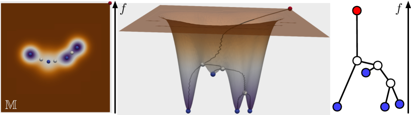
Figure 1: An example of a merge tree from a height field $f:{\mathbb{M}}\to{\mathbb{R}}$ defined on a 2D domain. From left to right: (a) 2D scalar field visualization with local minima in blue, saddles in white, and local maxima in red; (b) a merge tree embedded in the graph of the scalar field; and (c) an abstract (straight-line) visualization of a merge tree as a rooted tree equipped with the height function.

The construction of a merge tree for a given $f:{\mathbb{M}}\to{\mathbb{R}}$ is described procedurally as follows: we sweep the function value $a$ from $-\infty$ to $\infty$, and we create a new branch originating at a leaf node for each local minimum of $f$. As $a$ increases, such a branch is extended as its corresponding component in ${\mathbb{M}}_{a}$ grows until it merges with another branch at a saddle point. Assuming ${\mathbb{M}}$ is connected and $f$ achieves a unique global maximum, then all branches eventually merge into a single component, which corresponds to the root of the tree. For a given merge tree, leaves, internal nodes, and root node represent the minima, merging saddles, and global maximum of $f$, respectively. Fig. 1 displays a height function $f:{\mathbb{M}}\subset{\mathbb{R}}^{2}\to{\mathbb{R}}$ in (a), together with its corresponding merge tree embedded in the graph of the scalar field, i.e., $\{(x,f(x)):x\in{\mathbb{M}}\}$ in (b). Abstractly, a merge tree $T$ is a rooted tree equipped with $f$ restricted to its node set, $f:V\to{\mathbb{R}}$, as shown in (c).

3.2 Measure Networks and GW Distances

Gromov-Wasserstein (GW) distance, which we will define below, was introduced by Mémoli as a way to compare metric measure spaces [6, 7]. Sturm [15] and Peyré et al. [8] made the observation that GW distance gives a meaningful comparison between general square kernel matrices (i.e., not just distance matrices). This perspective was formalized mathematically by Chowdhury and Mémoli [9], who showed that a natural setting for generalized GW distance is as a metric on the space of measure networks. This level of generality will be most appropriate for our purposes, so we give an exposition of GW distance in this context, with a focus on the concrete setting of finite measure networks.

Measure networks. In its most general form, a measure network is a triple $(X,\mu,\omega)$: $X$ is a separable, completely metrizable space (i.e., a Polish space), $\mu$ is a fully supported Borel probability measure on $X$, and $\omega:X\times X\to{\mathbb{R}}$ a bounded, measurable function [9]. We adapt and simplify this formulation for our framework, which is focused specifically on measure networks arising from finite graphs. We then adapt this framework to a merge tree, considered to be a special case of a finite graph.

A finite graph $G$ may be represented as a measure network using a triple $(V,p,W)$: $V$ is the set of $n$ nodes in the graph, $p$ is a probability measure supported on the nodes of $G$, and $W\in\mathbb{R}^{|V|\times|V|}$ is a matrix that encodes relational information between the nodes. For example, $W$ may be a weighted adjacency matrix [11], a graph Laplacian [16], or a matrix of graph distances [41]. Without prior knowledge about $G$, $p$ is typically taken to be uniform; that is, $p(x)=1/n$, for each $x\in V$. We represent $p$ as a vector of size $n$, $p=\frac{1}{n}{\mathbf{1}_{n}}$, where ${\mathbf{1}_{n}}=(1,1,\dots,1)^{T}\in{\mathbb{R}}^{n}$. In the following sections, we slightly abuse the notation and identify a graph $G$ with a particular choice of measure network representation $(V,p,W)$.

GW distance. The key idea behind the GW distance is to find a probabilistic matching between a pair of measure networks by searching the convex set of couplings of the probability measures defined on the networks.

Let $G_{1}=(V_{1},p_{1},W_{1})$ and $G_{2}=(V_{2},p_{2},W_{2})$ be a pair of measure networks with $n_{1}$ and $n_{2}$ nodes, respectively. Let $[n]$ denote the set $\{1,2,\dots,n\}$ and suppose that $V_{1}=\{x_{i}\}_{i\in[n_{1}]}$ and $V_{2}=\{y_{j}\}_{j\in[n_{2}]}$. A coupling between probability measures $p_{1}$ and $p_{2}$ is a joint probability measure on $V_{1}\times V_{2}$ whose marginals agree with $p_{1}$ and $p_{2}$. That is, a coupling is represented as an $n_{1}\times n_{2}$ non-negative matrix $C$ such that $C{\mathbf{1}_{n_{2}}}=p_{1}$ and $C^{T}{\mathbf{1}_{n_{1}}}=p_{2}$. The set of all such couplings is denoted as ${\mathcal{C}}$, that is,

$${\mathcal{C}}={\mathcal{C}}(p_{1},p_{2})=\{C\in{\mathbb{R}}_{+}^{n_{1}\times n_{2}}\mid C{\mathbf{1}_{n_{2}}}=p_{1},C^{T}{\mathbf{1}_{n_{1}}}=p_{2}\}.$$ (1)

Following [9], the $q$-th GW distance between two measure networks is defined as

$$d^{GW}_{q}(G_{1},G_{2})=\frac{1}{2}\min_{C\in{\mathcal{C}}}\left(\sum_{i,j,k,l}|W_{1}(i,k)-W_{2}(j,l)|^{q}C_{i,j}C_{k,l}\right)^{1/q}.$$ (2)

The term $|W_{1}(i,k)-W_{2}(j,l)|$ is considered as the distortion of matching pairs of nodes $(x_{i},x_{k})$ in $G_{1}$ with $(y_{j},y_{l})$ in $G_{2}$. The minimizers in Eq. (2) are referred to as optimal couplings.

3.3 Fused Gromov-Wasserstein Distances

The fused Gromov-Wasserstein (FGW) distance is a hybrid between the Wasserstein distance from classical optimal transport and the GW distance discussed in Sect. 3.2.

A measure network $G=(V,p,W)$ may be equipped with additional information on its nodes, namely, the node attributes. That is, we associate each node $x\in V$ with an attribute $a$ in some attribute space – a metric space denoted as $(A,d_{A})$. Possible node attributes include labels on the nodes or information derived from the data domain from which $G$ arises.

Wasserstein distance. Classical optimal transport theory compares probability measures in terms of the Wasserstein distance $d_{W}$. Given a pair of measure networks $G_{1}=(V_{1},p_{1},W_{1})$ and $G_{2}=(V_{2},p_{2},W_{2})$, where nodes $x_{i}\in V_{1}$ and $y_{j}\in V_{2}$ are equipped with attributes $a_{i}$ and $b_{j}$ within the same attribute space, we define their $q$-th Wasserstein distance based on distances between node attributes to be

$$d^{W}_{q}(G_{1},G_{2})=\min_{C\in{\mathcal{C}}}\left(\sum_{i,j}d_{A}(a_{i},b_{j})^{q}C_{i,j}\right)^{1/q}.$$ (3)

We refer to $d_{A}(a_{i},b_{j})$ as the attribute distance between nodes $x_{i}\in V_{1}$ and $y_{j}\in V_{2}$.

FGW distance. Vayer et al. introduced the fused Gromov-Wasserstein (FGW) distance between attributed graphs and other structured objects [40, 42]. We describe their framework in the setting of measure networks. In a nutshell, the FGW distance is a trade-off between the Wasserstein distance in Eq. (3) and the GW distance in Eq. (2).

For $q\in[1,\infty)$ and a trade-off parameter $\alpha\in[0,1]$, the FGW distance $d_{FGW}$ between attributed measure networks $G_{1}$ and $G_{2}$ is defined (following [40]) as

$$d^{FGW}_{q}(G_{1},G_{2})=$$ (4)

$$\min_{C\in{\mathcal{C}}}\sum_{i,j,k,l}[(1-\alpha)d_{A}(a_{i},b_{j})^{q}+\alpha|W_{1}(i,k)-W_{2}(j,l))|^{q}]C_{i,j}C_{k,l}.$$ (5)

Here, $C$ is considered as a soft assignment matrix, and $\alpha$ gives a trade-off between labels and structures. As shown in Sect. 4, Eq. (5) plays an important role in encoding both intrinsic and extrinsic information for merge tree comparisons.

The FGW distance enjoys a number of desirable properties (see [40] and its supplementary material, as well as [21]). Specifically, it interpolates between the Wasserstein distance on the labels and GW distances on the structures:

Theorem 1.

[40, Theorem 3.1] As $\alpha\to 0$, the FGW distance recovers the Wasserstein distance,

$$\lim_{\alpha\to 0}d^{FGW}_{q}=(d^{W}_{q})^{q}.$$ (6)

As $\alpha\to 1$, the FGW distance recovers the GW distance (ignoring the constant factor in Eq. (2)),

$$\lim_{\alpha\to 1}d^{FGW}_{q}=(d^{GW}_{q})^{q}.$$ (7)

Furthermore, $d^{FGW}_{q}$ defines a metric for $q=1$ and a semimetric for $q\geq 2$ (i.e., the triangular inequality is relaxed by a factor $2^{q-1}$) [40, Theorem 3.2].

For the remainder of the paper, we work with $d^{FGW}_{q}$ for $q=2$. For easy reference, we have

$$d^{FGW}_{2}(G_{1},G_{2})=$$

$$\min_{C\in{\mathcal{C}}}\sum_{i,j,k,l}[(1-\alpha)d_{A}(a_{i},b_{j})^{2}+\alpha|W_{1}(i,k)-W_{2}(j,l))|^{2}]C_{i,j}C_{k,l}.$$ (8)

The choice of $q=2$ is justified for computational reasons: given two measure networks with $n_{1}$ and $n_{2}$ nodes respectively, we can simplify the computation of the tensor product involved in the evaluation of the GW loss from $\mathcal{O}(n_{1}^{2}n_{2}^{2})$ to $\mathcal{O}(n_{1}n_{2}^{2}+n_{1}^{2}n_{2})$ when considering $q=2$ [8].

3.4 Partial Wasserstein and Partial GW Distances

Our final ingredient comes from partial optimal transport (see, e.g., [43, 44, 45]). We review the framework of Chapel et al. [22] that studies partial Wasserstein and partial GW distances. Notations are simplified in our setting of measure networks. A major drawback of classical optimal transport is that it requires that all mass be transported. This requirement may be too restrictive for many applications where “mass changes may occur due to a creation or an annihilation while computing an optimal transport plan” [22]. In the setting of feature tracking, we need to account for mass changes due to the appearances and disappearances of features.

Partial Wasserstein distance. Partial optimal transport focuses on transporting a fraction $0\leq m\leq 1$ of the mass as cheaply as possible [22]. The set of admissible couplings is defined to be

$${\mbox{$\mathcal{C}$}}_{m}={\mathcal{C}}_{m}(p_{1},p_{2})$$

$$=\{C\in{\mathbb{R}}_{+}^{n_{1}\times n_{2}}\mid C{\mathbf{1}_{n_{2}}}\leq p_{1},C^{T}{\mathbf{1}_{n_{1}}}\leq p_{2},\mathbf{1}_{n_{1}}^{T}C{\mathbf{1}_{n_{2}}}=m\},$$ (9)

and the partial $q$-Wasserstein distance is defined as

$$d^{pW}_{q}(G_{1},G_{2})=\min_{C\in{\mathcal{C}}_{m}}\left(\sum_{i,j}d_{A}(a_{i},b_{j})^{q}C_{i,j}\right)^{1/q}.$$ (10)

A main difference between partial Wasserstein distance and Wasserstein distance is that we replace the equalities in Eq. (1) with inequalities in Eq. (3.4) to account for “partial mass transport”.

Partial GW distance. In a similar fashion, given the set of admissible couplings ${\mathcal{C}}_{m}$, the partial q-GW distance is defined as

$$d^{pGW}_{q}(G_{1},G_{2})=\frac{1}{2}\min_{C\in{\mathcal{C}}_{m}}\left(\sum_{i,j,k,l}|W_{1}(i,k)-W_{2}(j,l)|^{q}C_{i,j}C_{k,l}\right)^{1/q}.$$ (11)

4 Method

We now describe our novel framework that performs feature tracking with partial optimal transport. We first introduce a new, partial Fused Gromov-Wasserstein (pFGW) distance between a pair of measure networks (Sect. 4.1). We then model and compare merge trees as measure networks (Sect. 4.2). The pFGW distance gives rise to a partial matching between topological features (i.e., critical points) in merge trees, thus enabling flexible topology tracking for time-varying data (Sect. 4.3).

4.1 Partial Fused Gromov-Wasserstein Distance

For topology-based feature tracking, oftentimes features (i.e., critical points) will appear and disappear in time-varying data. Features that appear at time $t$ do not need to be matched with features at time $t-1$; similarly, features that disappear at time $t$ do not need to be matched with features at time $t+1$. Therefore, we need to introduce a partial Fused Gromov-Wasserstein (pFGW) distance for feature tracking to handle the appearances and disappearances of multiple features in time-varying data.

The pFGW distance is defined based on the set of admissible couplings ${\mathcal{C}}_{m}$ in Eq. (3.4) and the FGW distance in Eq. (5). Given a pair of measure networks $G_{1}$ and $G_{2}$, formally, we have

$$d^{pFGW}_{q}(G_{1},G_{2})=$$

$$\min_{C\in{\mathcal{C}}_{m}}\sum_{i,j,k,l}[(1-\alpha)d_{A}(a_{i},b_{j})^{q}+\alpha|W_{1}(i,k)-W_{2}(j,l))|^{q}]C_{i,j}C_{k,l}.$$ (12)

Notice that the newly defined pFGW distance is not too different from the FGW distance, except that it is more flexible by allowing a $m$ fraction of the total mass to be transported. In practice, we set $q=2$ and work with $d^{pFGW}_{2}$.

We remark that a related distance was recently introduced in [46] and applied to brain anatomy alignment. The difference between the two distances is that [46] employs a different notion of partial optimal transport (rather, unbalanced optimal transport), where the coupling set is expanded to all joint probability measures and disagreement of marginals is penalized by Kullback-Liebler (KL) divergence. In [46], instead of choosing the amount of mass to be preserved, one must tune the relative weight of the KL regularization term.

Computing pFGW distance. Computing the pFGW distance is a slight modification of the FGW computation in [21] with ingredients of the Frank-Wolfe optimization algorithm [47] for partial GW computation [22]. On a high-level, computing the partial Wasserstein and the partial GW distances relies on adding dummy nodes in the transportation plan and allowing such dummy nodes to “absorb” a fraction of the mass during transportation. With these dummy nodes added onto the marginals, the Frank-Wolfe algorithm then solves an iterative first-order optimization for constrained convex optimization. Our implementation is based on a minor modification of the code for the FGW framework in [40] (https://github.com/tvayer/FGW) with components from the partial optimal transport solvers, part of the open-source Python library for optimal transport [48] (https://pythonot.github.io/gen_modules/ot.partial.html).

4.2 Modeling Merge Trees as Measure Networks

Unless otherwise specified, we represent a merge tree $T$ as an attributed measure network $(V,p,W)$ for the remainder of this paper, where the attributes, weight matrix $W$, and probability measure $p$ are defined below.

Given a merge tree $T=(V,p,W)$, information that is typically topological and intrinsic to a merge tree, such as tree distances, may be encoded via the weight matrix $W$ and the probability measure $p$ (Sect. 4.2.1). Information that is extrinsic to a merge tree may be encoded via the node labels $(A,d_{A})$. Extrinsic information is typically geometrical or statistical, and arises from the data domain, such as the coordinates of the critical points of $f:{\mathbb{M}}\to{\mathbb{R}}$ (that give rise to the merge tree), function values $f$ restricted to the set of nodes $V$, and prior knowledge (such as labels) associated with nodes in a measure network.

We discuss various strategies that encode extrinsic and intrinsic information for merge tree comparisons. The key takeaway is that the pFGW distance we build upon provides a flexible framework that encodes geometric and topological information for comparative analysis of merge trees.

4.2.1 Encoding Intrinsic Information

A merge tree $T$ is represented using a triple $(V,p,W)$. Information intrinsic to $T$ may be encoded via $p$ and $W$ as we now describe.

Encoding edge information. Recall that a merge tree $T$ is a tree equipped with a function $f:V\to{\mathbb{R}}$ defined on its nodes $V$. To encode the information of $f$, we explore a shortest path (SP) strategy. Recall that each node $x$ in $T$ is associated with a scalar value $f(x)$. Using the SP strategy, for $x,x^{\prime}\in V$, we define $W(x,x^{\prime})$ as follows: we associate the weight $W(x,x^{\prime})=|f(x)-f(x^{\prime})|$ with each pair of adjacent nodes; for nonadjacent nodes, $W(x,x^{\prime})$ is the sum of the edge weights along the unique shortest path in $T$ from $x$ to $x^{\prime}$. By construction, the shortest path between two nodes goes through their lowest common ancestor in $T$. That is, an ancestor of a node $x$ in $T$ is any node $v$ such that there exists a path from $x$ to $v$ where $f$-values are nondecreasing along the path. The lowest common ancestor of two nodes $x,x^{\prime}$, denoted ${\mathrm{lca}}(x,x^{\prime})$, is the common ancestor of $x$ and $x^{\prime}$ with the lowest $f$-value.

We explore an additional strategy by encoding the function values of the lowest common ancestors among pairs of nodes, referred to as the lowest common ancestor (LCA) strategy. Using the LCA strategy, we define $W(x,x^{\prime})=f({\mathrm{lca}}(x,x^{\prime}))$ for $x,x^{\prime}\in V$. For a given ordering of vertices, $W$ is also known as the induced ultra matrix of a merge tree [19].

Encoding node information. Without prior knowledge, we may define $p$ as a uniform measure, i.e., $p=\frac{1}{|V|}{\mathbf{1}_{|V|}}$. This uniform strategy means that all nodes in the merge trees are considered to be equally important during merge tree comparison and matching.

On the other hand, $p$ could be made more general by giving higher weights to nodes deemed more important by an application. For example, we may assign each node $x\in V$ an importance value that is proportional to the functional difference to its parent node, ${\mathrm{parent}}(x)$, which is the unique neighbor $x^{\prime}$ of $x$ in $T$ with $f(x^{\prime})\geq f(x)$. That is, we set $p(x)\propto(f({\mathrm{parent}}(x))-f(x))$. Such assignment is referred to as the parent strategy.

4.2.2 Encoding Extrinsic Information

Extrinsic information that typically arises from the geometry of the data domain may be encoded via the attribute space $(A,d_{A})$ and attribute distance $d_{A}$ in Eq. (5). For a node in the merge tree, the assigned attribute may be a high-dimensional vector or a categorical label. Given a pair of merge trees $T_{1}=(V_{1},p_{1},W_{1})$ and $T_{2}=(V_{2},p_{2},W_{2})$, nodes $x_{i}\in V_{1}$ and $y_{j}\in V_{2}$ are equipped with attributes $a_{i}$ and $b_{j}$ from the same attribute space $(A,d_{A})$.

These attributes may be coordinates associated with critical points in the data domain. Specifically, assume $x_{i}\in V_{1}$ corresponds to a critical point of a function $f_{1}:{\mathbb{M}}\to{\mathbb{R}}$ in the data domain ${\mathbb{M}}$ with coordinates $(x^{1}_{i},x^{2}_{i})$ (assuming ${\mathbb{M}}\subset\mathbb{R}^{2}$), whereas $y_{j}\in V_{2}$ corresponds to a critical point of $f_{2}:{\mathbb{M}}\to{\mathbb{R}}$ with coordinates $(y^{1}_{j},y^{2}_{j})$. By setting $a_{i}=(x^{1}_{i},x^{2}_{i})$ and $b_{j}=(y^{1}_{j},y^{2}_{j})$, we define $d_{A}$ to be the Euclidean distance between $a_{i}$ and $b_{j}$, $d_{A}(a_{i},b_{j})=\sqrt{(x^{1}_{i}-y^{1}_{j})^{2}+(x^{2}_{i}-y^{2}_{j})^{2}}$. This definition is referred to as the coordinates strategy. This strategy is a natural choice because a core method for critical point tracking is often based on their Euclidean distance proximity.

4.2.3 Simple Examples

In Fig. 2, we show a simple example of using pFGW distance for critical point matching between a pair of merge trees $T_{1}$ and $T_{2}$. These merge tree arise from slightly different mixtures of Gaussian functions $f_{1}$ and $f_{2}$ in 2D; see (a) and (c), respectively. As shown in (a), $T_{1}$ and $T_{2}$ are structurally similar: $T_{1}$ contains $10$ critical points, and $T_{2}$ has $8$ critical points with a pair of critical points removed (see the region enclosed by the red box). Here, we apply a uniform strategy to $p$. We set $m=0.8$, since we suspect that only 8 of 10 nodes in $T_{1}$ could find its proper match in $T_{2}$. After computing the pFGW distance, the $10\times 8$ coupling matrix $C$ is shown in (d) and visualized in (b). An entry $C(i,j)$ in the coupling matrix indicates the probability of a node $i\in T_{1}$ being matched to node $j\in T_{2}$. In particular, rows $C(2,\cdot)$ and $C(3,\cdot)$ (in a red box) are both zero, indicating that no partners in $T_{2}$ are matched with nodes $2$ and $3$ in $T_{1}$. In other words, by design, nodes $2$ and $3$ in $T_{1}$ are matched to a dummy node during the partial optimal transport. Furthermore, nodes in $T_{2}$ are colored by its most probable partner in $T_{1}$, which aligns well with our intuition. In this example, each node in $T_{1}$ has a unique partner in $T_{2}$; however, in practice, a node may be coupled with multiple nodes with nonzero probabilities, as shown in the next example.

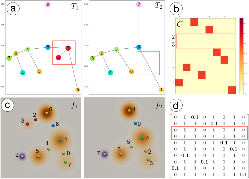
Figure 2: Partial optimal matching using pFGW, $m=0.8$. (a) Merge trees that arise from mixtures of Gaussian functions in (c). The coupling matrix (d) is visualized with a heat map in (b).

We provide another example in Fig. 3 to demonstrate probabilistic matching with our framework. As shown in (b), $f_{1}$ is a mixture of four positive and one negative Gaussian functions. In $f_{2}$, a positive Gaussian function on top is split into two Gaussian functions, resulting in two local maxima and one saddle point. Merge trees $T_{1}$ and $T_{2}$ in (a) describe the topology of scalar fields $f_{1}$ and $f_{2}$, respectively. Notice that the topological change in $T_{2}$ (enclosed by a red box) highlights the feature splitting event in $f_{2}$. Rather than enforcing a one-to-one correspondence between the critical points, our pFGW framework allows probabilistic matching among them. As shown in (c)-(d), the coupling matrix $C$ contains multiple rows and columns with more than one nonzero entries. For example, the row $C(3,\cdot)$ (red box) has two nonzero entries, namely $0.025$ at $C(3,1)$ and $0.01$ at $C(3,4)$, see (d), which indicates that node $3$ in $T_{1}$ can be matched to both node $1$ and $4$ in $T_{2}$ with varying probabilities. Such a matching is probable due to the feature splitting event. As node $4$ in $T_{2}$ is closer to node $3$ in $T_{1}$ (than node $1$ in $T_{2}$), $C(3,4)$ has a higher coupling probability than $C(3,1)$.

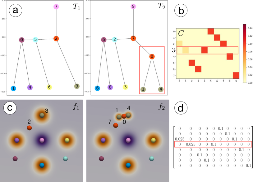
Figure 3: Partial optimal matching using pFGW, $m=0.85$. (a) Merge trees that arise from mixtures of Gaussian functions in (c). The coupling matrix (d) is visualized with a heat map in (b).

4.3 Flexible Topology Tracking

By modeling merge trees as measure networks (Sect. 4.2) and introducing a new pFGW distance based on partial optimal transport (Sect. 4.1), we are ready to describe our topology tracking framework in Sect. 4.3.1 and discuss its flexibility in Sect. 4.3.2.

4.3.1 Tracking Framework

Our topology tracking framework consists of three steps.

1. Feature detection. First, we compute a merge tree for each time step. We use the algorithm implemented in TTK [49]. Since each of our datasets is a 2D time-varying scalar field, each merge tree contains local minima, saddles, and a global maximum (assuming there is a unique global maximum). When the data is noisy, we apply persistent simplification [50] to remove pairs of critical points with low persistence. In other words, we retain significant features in the domain for tracking purposes.

2. Feature matching. Second, we utilize our pFGW framework for feature matching across adjacent time steps. Let $T_{1}$ and $T_{2}$ be two merge trees computed at time steps $t$ and $t+1$, respectively. We then model them as measure networks $T_{1}=(V_{1},p_{1},W_{1}),T_{2}=(V_{2},p_{2},W_{2})$ and apply the pFGW framework described in Sect. 4.1 to match critical points from $T_{1}$ with $T_{2}$.

We utilize a conservative bijective matching strategy. Based on the optimal coupling $C$, a node $x\in V_{1}$ may be coupled (matched) with multiple nodes in $V_{2}$. We will choose $x^{\prime}\in V_{2}$, which has the highest matching probability with $x$ (referred to as the most probable partner). Similarly, for $x^{\prime}\in V_{2}$, we will choose its most probable partner $x^{\prime\prime}\in V_{1}$. If $x=x^{\prime\prime}$, and then $x$ and $x^{\prime}$ are matched to form a trajectory.

3. Trajectory extraction. Trajectories are constructed by connecting successively matched critical points. For any two adjacent time steps $t$ and $t+1$, if a node $x$ at time $t$ is matched with a node $x^{\prime}$ at time $t+1$, then a segment is constructed connecting $x$ and $x^{\prime}$ in the spacetime domain. If a node $x$ at time $t$ is ignored (i.e., matched to the dummy node) during the partial optimal transport, then the current trajectory terminates. If a node $x^{\prime}$ at time $t+1$ is ignored during the partial optimal transport, it is considered as a new feature, and a new trajectory begins.

4.3.2 A Discussion on Flexibility

Modeling a merge tree $T$ as a measure network $T=(V,p,W)$ and its associated pFGW distance offers great flexibility in the comparative analysis of merge trees. The flexibility is reflected via a number of parameters.

First, parameters $W$ and $p$ allow various strategies for encoding intrinsic and extrinsic information of a merge tree, including the shortest path (SP) and lowest common ancestor (LCA) strategies for encoding edge information; uniform and parent strategies for encoding node information; and coordinates strategy for encoding geometric information from the data domain.

Second, parameter $\alpha$ from Eq. (12) strikes a balance in considering intrinsic information (via the GW distance) and extrinsic information (via the Wasserstein distance) for merge tree comparisons.

Third, parameter $m$ from Eq. (12) allows partial mass transport to accommodate the appearances and disappearances of topological features.

5 A New Stability Result

We now state a new theoretical stability result involving the GW distance, which shows that a small change in the function data produces a small change in merge tree representations, as measured by the GW distance; see the supplementary material for a detailed proof and some experimental validation of Theorem 2.

Let $X$ be a finite, connected geometric simplicial complex with vertex set $V$. Let $f:X\to\mathbb{R}$ be a function obtained by starting with a function $f:V\to\mathbb{R}$ on the vertex set and extending linearly over higher dimensional simplices. Let $p$ be a probability distribution over the vertex set $V$. We will assume that $p$ is balanced, in the sense that for any $u,v,w\in V$, we have $p(u)\cdot p(v)\leq p(w)$; this property holds for the uniform distribution, for example. We then define the measure network representation of $T_{f}$ to be $G_{f}=(V,p,W_{f})$, with $W_{f}$ defined based on the least common ancestor (LCA) strategy. We also define a family of weighted norms on the space of functions $f:V\to\mathbb{R}$ by

$$\|f\|_{L^{q}(p)}:=\left(\sum_{v\in V}|f(v)|^{q}p(v)\right)^{1/q}.$$

We can now state our theorem.

Theorem 2.

Let $f,g:X\to\mathbb{R}$ be functions defined as above and let $p$ be a balanced probability distribution. Then

$$d^{GW}_{q}(G_{f},G_{g})\leq\frac{1}{2}|V|^{2/q}\|f-g\|_{L^{q}(p)}.$$

We also show in the supplementary material that the Lipschitz constant $\frac{1}{2}|V|^{2/q}$ is asymptotically tight for general probability measures. When the measure is uniform, the constant can be improved to $\frac{1}{2}|V|^{1/q}$. Finally, we have the following corollary, which treats the shortest path strategy for encoding a merge tree as a measure network.

Corollary 1.

Let $f,g:X\to\mathbb{R}$ be functions defined as above and let $p$ be a balanced probability distribution. Let $G_{f}$ (respectively, $G_{g}$) denote the representation of the merge tree $T_{f}$ ($T_{g}$) defined by the shortest path strategy. Then

$$d^{GW}_{q}(G_{f},G_{g})\leq\left(|V|^{2/q}+2\right)\|f-g\|_{L^{q}(p)}.$$

6 Experiments

We demonstrate the utility of our framework with four 2D datasets and one 3D dataset. For each dataset, we also compare against two state-of-the-art approaches.

6.1 Datasets Overview

The first dataset is a simulation of a 2D flow generated by a heated cylinder using the Boussinesq approximation [51, 52], referred to as the $\mathsf{Heated\,Cylinder}$ dataset. The simulation was done with a Gerris flow solver and was resampled onto a regular grid. It shows a time-varying turbulent plume containing numerous small vortices that, in part, rotate around each other. We generate a set of merge trees from the magnitude of the velocity fields based on $31$ time steps ($600$-$630$ from the original $2000$ time steps). These time steps describe the evolution of small vortices.

The second dataset is a 2D unsteady cylinder flow (synthetic), referred to as the $\mathsf{Unsteady\,Cylinder\,Flow}$ dataset. This synthetic vector field represents a simple model of a von-Kárman vortex street generation and was constructed by Jung, Tel, and Ziemniak as co-gradient to a stream function [53]. The obstacle is positioned at $(0,0)$ and has a radius of $1$. In the LIC image on the side, the flow in the interior of the obstacle has not been set to zero. Note that only two vortices are present at the same time. We sampled four periods onto a regular grid. We use the first 499 time steps in the dataset, and use merge trees computed for the velocity magnitude field that primarily capture the behavior of local maxima, saddles, and a global minimum. The first two datasets are available via the Computer Graphics Laboratory [54].

The third dataset is the classic 2D von Kárman vortex street dataset coming from the simulation of a viscous 2D flow around a cylinder, referred to as the $\mathsf{Vortex\,Street}$ dataset. It contains vortices moving with almost constant speed to the right, except directly in the wake of the obstacle, where they accelerate. We model vorticity as scalar fields, and track the evolution of local maxima over time.

The fourth dataset comes from the 2008 IEEE Visualization Design Contest [55], referred to as the $\mathsf{Ionization\,Front}$ dataset. This time-varying dataset simulates the propagation of an ionization front instability. The simulation is done with 3D radiation hydrodynamical calculations of ionization front instabilities in which multifrequency radiative transfer is coupled to the primordial chemistry of eight species [56]. For this experiment, we use the density to generate merge trees from the 2D slices near the center of the simulation volume for 123 time steps, which correspond to steps 11-133 from the original 200 time steps. These time steps show the density over time as the instability progresses toward the right.

Finally, we use a collection of 3D volumes simulating the wind velocity magnitude of the Isabel hurricane, referred to as the $\mathsf{Isabel}$ dataset. We use this dataset to demonstrate the ability of our method to track features in 3D scientific datasets. We use $12$ time steps that depict the key events of the hurricane (formation, drift, and landfall): time steps $2$ to $5$, $30$ to $33$, and $45$ to $48$. This 3D dataset is acquired from the Climate Data Gateway at NCAR [57].

6.2 Heated Cylinder Dataset

We first use the $\mathsf{Heated\,Cylinder}$ dataset to demonstrate in detail our parameter tuning process in Sect. 6.2.1. We then showcase the tracking results based on partial optimal transport in Sect. 6.2.2. Finally, we compare against previous approaches in Sect. 6.2.3.

6.2.1 Parameter Tuning

There are two types of parameters in our framework: the preprocessing parameter $\epsilon$ that is used to de-noise the input data; and the in-processing parameters $W$, $p$, $\alpha$, and $m$ for feature tracking.

Preprocessing parameter tuning. Persistence simplification is considered a preprocessing step for data de-noising. Let $\epsilon\in[0,1]$ denote the persistence simplification parameter. Let $R$ denote the range of a given scalar field. Using persistence simplification, critical points with persistence less than $\epsilon\cdot R$ are removed from the domain. $\epsilon$ is typically chosen based on the shape of a persistence graph, where a plateau in a persistence graph indicates a stable range of scales to separate features from noise. Such a strategy has been used perviously in simplifying scientific data (e.g., [58, 59]). For $\mathsf{Heated\,Cylinder}$, we use $\epsilon=6\%$, which is slightly left of the first observable plateau in the persistence graph, as we try to maintain a slightly larger number of features; see Fig. 4.

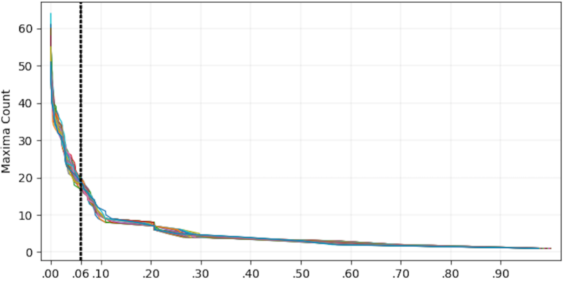
Figure 4: $\mathsf{Heated\,Cylinder}$: persistent simplification $\epsilon=6\%$; x-axis is $\epsilon$.

In-processing parameter tuning. To evaluate the quality of the extracted trajectories, we aim to reduce two types of artifacts during parameter tuning: oversegmentations where a single trajectory is unnecessarily segmented into subtrajectories; and mismatches between critical points that appear as zigzag patterns connecting adjacent time steps.

We introduce two metrics to evaluate these artifacts quantitatively: first, the number of trajectories, denoted as $N$; and second, the maximum Euclidean distance between matched critical points across time (referred to as the maximum matched distance for simplicity), denoted as $L$. Specifically, we introduce a parameter $L^{*}$ that represents an upper bound on $L$. During parameter tuning, a guiding principle is to reduce oversegmentations and mismatches by minimizing $N$ and $L$. In this paper, we focus on tracking features surrounding local maxima; therefore, we compute $N$ and $L$ only for local maxima trajectories.

First, we consider parameter tuning for $W$ and $p$. We inspect the behavior of $W$ (or $p$) while keeping other parameters fixed. Through extensive experiments across all datasets in this paper, we observe that the SP (i.e., shortest path) strategy for $W$ generally behaves equal to or better than the LCA strategy in minimizing $N$ and $L$. We also observed that the uniform strategy for $p$ performs better than the parent strategy. Therefore, for the rest of the paper, $W$ uses the SP strategy and $p$ uses the uniform strategy.

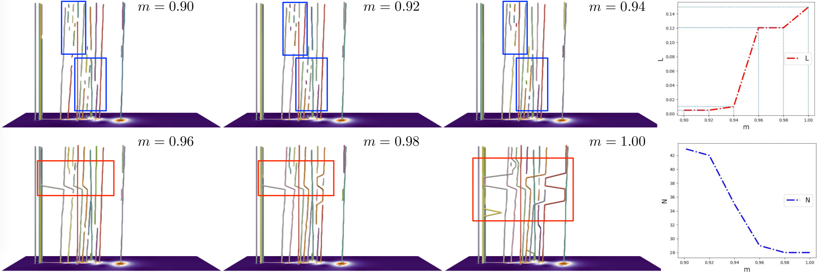
Figure 5: $\mathsf{Heated\,Cylinder}$. Left: for a fixed $\alpha=0.1$, perform a grid search of $m$ and observe the number of oversegmentations (in blue boxes) and mismatches (in red boxes). Right: the trend among the number of trajectories ($N$) and the maximum matched distance ($L$) as $m$ increases.

Second, we study the parameter tuning of $m$ for a fixed $\alpha$. $m$ may be considered as an in-processing step for data de-noising, by matching a certain number of features to the dummy nodes during partial optimal transport. We use an example in Fig. 5 (left) to demonstrate the process. For a fixed $\alpha=0.1$, we perform a grid search of $m\in[0.5,1.0]$ with an increment of $0.01$. For instance, at $m=0.90$, we see a number of oversegmented trajectories in the blue boxes; such oversegmentations decrease as $m$ increases from $0.90$ to $0.94$ (top left). On the other hand, obvious mismatches appear in the red boxes for $m\geq 0.96$ (bottom left). As $m$ increases from $0.9$ to $1.0$, we observe a decrease in the number of trajectories $N$ and an increase in the maximum matched distance $L$; this is additionally demonstrated in the plots of $N$ and $L$, see Fig. 5 (top right and bottom right). If our goal is to choose an appropriate global value for $m$, then we are interested in striking a balance between minimizing $N$ and minimizing $L$; therefore, we may choose $m=0.94$ in this example. However, as shown in Fig. 5, at $m=0.94$, there are still oversegmentations within the blue box, indicating that a locally adaptive value of $m$ might be more appropriate in practice.

Our final strategy aims to automatically adjust the value of $m$ between adjacent time steps to reduce $N$, without increasing $L$ drastically. Specifically, we perform a 2D grid search of $\alpha$ and $m$: $\alpha\in[0.0,1.0]$ with an increment of $0.1$, and $m\in[0.5,1.0]$ with an increment of $0.01$. For each fixed $\alpha$, we apply the following procedure. First, we plot the curve of $L$ as we increase $m$. Second, we apply the elbow method and pick the elbow of the $L$ curve as an upper bound on $L$, denoted as $L^{*}$. Finally, for each pair of adjacent steps $t$ and $t+1$, we automatically choose the largest value of $m$ such that $L$ does not exceed $L^{*}$. In other words, $m$ varies adaptively across time steps, see Fig. 6 (top) with marked elbow points.

As $\alpha$ varies, we plot the number of trajectories $N$ and the maximum matched distance $L$ ($\leq L^{*}$) at each $\alpha$, as shown in Fig. 6 (bottom). We look for a proper value of $\alpha$ to minimize both $N$ and $L$. However, $N$ and $L$ may not be minimized at the same $\alpha$. In this scenario, we look for an $\alpha$ such that it minimizes $N$ while keeping $L$ to be small enough to minimize the number of mismatches. Using this strategy, we set $\alpha=0.1$, with a corresponding $L^{*}=0.00997$.

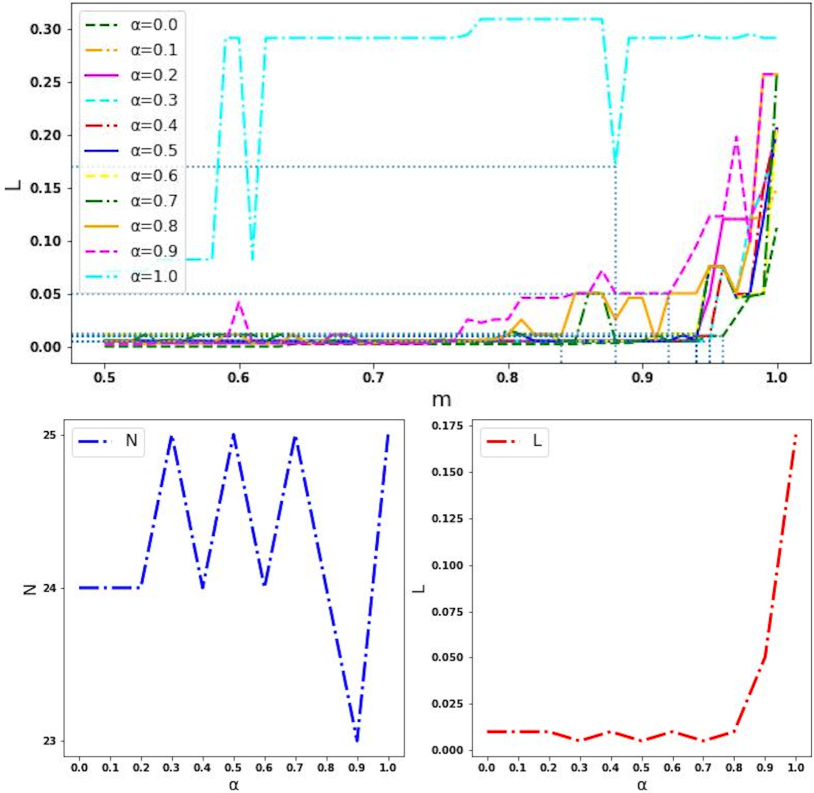
Figure 6: $\mathsf{Heated\,Cylinder}$. (a) $L$ as we change the global $m$ for each $\alpha$; elbows of curves are marked with dotted horizontal and vertical lines, (b) $N$ and $L$ with respect to $\alpha$ (using adaptive $m$).

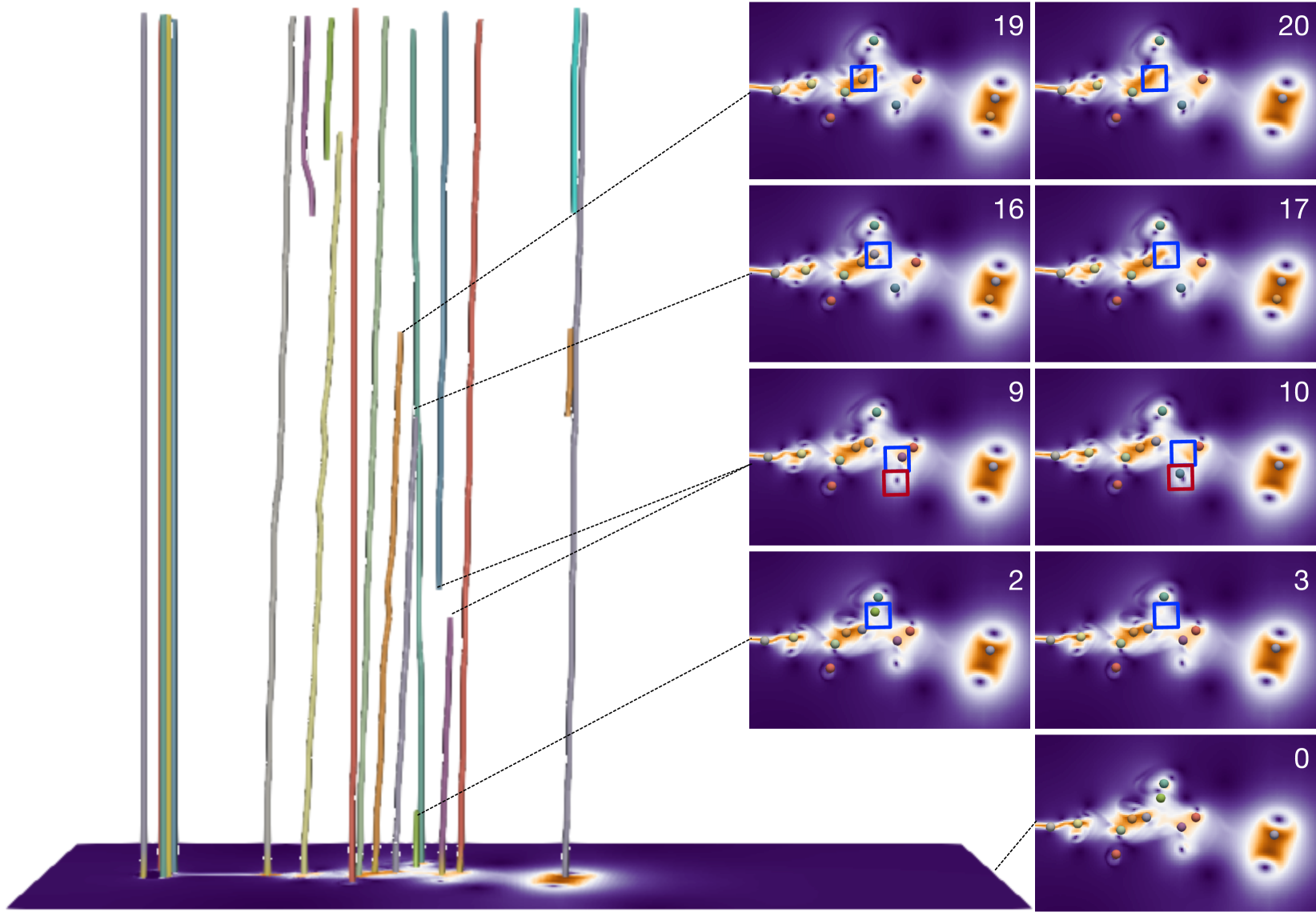
Figure 7: $\mathsf{Heated\,Cylinder}$. Tracking result (left) with views of scalar fields (right) that capture topological changes in the time-varying scalar field at selected time steps. The appearances and disappearances of critical points are highlighted in red and blue boxes, respectively.

6.2.2 Tracking Result

Fig. 7 shows our final tracking result on the left with views of scalar fields on the right that highlight the appearances and disappearances of critical points. In Fig. 7 (left), the $xy$-plane visualizes the scalar field at $t=0$, and the $z$-axis shows the trajectories for all the local maxima and the global minimum as time increases. Most trajectories are shown to be straight lines as only minor topological changes occur in this dataset. Meanwhile, our framework successfully captures the appearances and disappearances of critical points. As shown in Fig. 7 (right), for time steps $2\to 3,10\to 11,16\to 17$ and $19\to 20$, critical points disappear in the blue boxes, resulting in the termination of trajectories; for time steps $9\to 10$, a critical point appears in a red box, resulting in the start of a new, green trajectory.

6.2.3 Comparison with Previous Approaches

We compare the tracking results for our pFGW framework with two other state-of-the-art feature tracking approaches, referred to as Global Feature Tracking (GFT) [29, 30] and Lifted Wasserstein Matcher [25] (LWM); see the supplementary material for parameter tuning of GFT and LWM.

Implementations. Our pFGW framework utilizes the libraries implemented in TTK [49] for merge tree computation. GFT is implemented in C++ and is available at [60]. It computes the merge trees and region segmentations, and outputs the tracking results between critical points at adjacent time steps. GFT allows tracking between saddles and local extrema, whereas pFGW only focuses on tracking between local extrema. Therefore, we adjust the postprocessing of GFT to remove trajectories involving saddles. LWM is implemented as an embedded library in TTK. Results of all three methods are visualized via ParaView [61] with VTK [62].

Since neither LWM nor GFT includes details on their parameter tuning, we apply the same parameter tuning strategy as pFGW to both LWM and GFT, that is, minimizing the number of trajectories and the maximum matched distances; see the supplementary material for details.

Furthermore, all three methods apply the same persistence-based simplification during preprocessing. However, since GFT is defined on a regular grid of squares, and pFGW and LWM use identical simplicial meshes, we expect minor inconsistencies on the simplified datasets between GFT and other two methods.

Tracking Results Comparison. All three tracking results are shown in Fig. 8 (top). All three methods produce $24$ trajectories, but there are noticeable differences in GFT-produced trajectories (comparing red and blue boxes, respectively). We evaluate these results quantitatively based on observable oversegmentations and mismatches. There are obvious oversegmentations from GFT compared to the other two methods: a trajectory in the red box is broken in GFT, but remains continuous in pFGW and LWM.

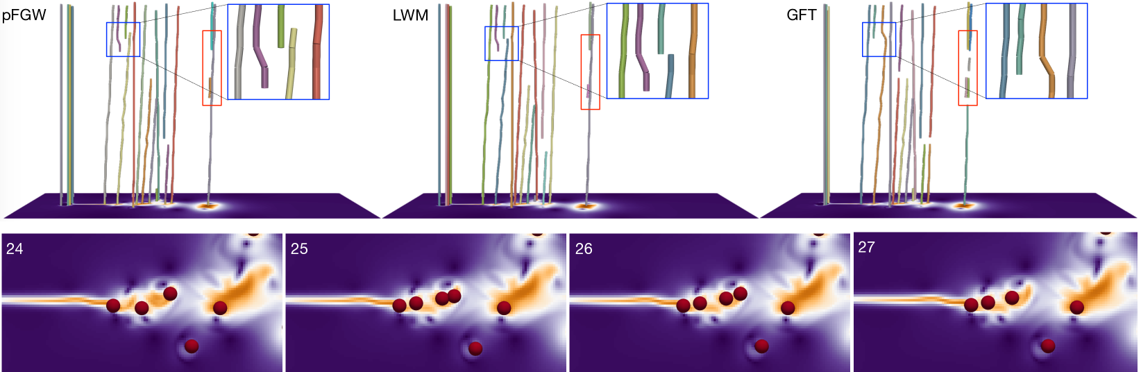
Figure 8: $\mathsf{Heated\,Cylinder}$. Top: from left to right, pFGW (ours), LWM, and GFT, respectively. Bottom: the appearances and disappearances of local maxima in the blue boxes on top.

As for mismatches, GFT produces a different tracking result from pFGW and LWM in the blue box, from time steps $24\to 27$; the corresponding scalar fields are shown in Fig. 8 (bottom). We interpret the topological changes as follows: a critical point appears from $24\to 25$, another critical point appears from $25\to 26$, and a critical point disappears from $26\to 27$. The trajectories in pFGW and LWM correctly reflect these topological changes, whereas those in GFT consider these changes to be the movements of critical points. Therefore, pFGW and LWM perform similarly, but GFT performs slightly worse for the $\mathsf{Heated\,Cylinder}$ dataset.

6.3 Unsteady Cylinder Flow

For the $\mathsf{Unsteady\,Cylinder\,Flow}$ dataset, we employ the same parameter tuning strategy detailed in Sect. 6.2.1. We use a persistence simplification level at $\epsilon=1\%$. We set $\alpha=0.1$ and $L^{*}=0.03768$, see the supplementary material for details.

6.3.1 Tracking Results

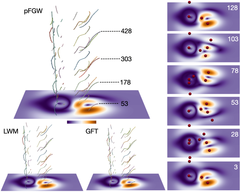
Figure 9: $\mathsf{Unsteady\,Cylinder\,Flow}$. Left: comparing tracking results for pFGW, LWM, and GFT, respectively. Right: snapshots of scalar fields within a single period between $t=3$ and $t=128$.

Our tracking result using pFGW is highly periodic, where the extracted trajectories exhibit repetitive patterns that include the appearances, disappearances, and movements of local maxima over time, see Fig. 9 (left). We show a few time steps at $t=53,178,303$, and $428$ to highlight a periodicity of $\approx 125$. Furthermore, as shown in Fig. 9 (right), six snapshots show the evolution of the scalar field within a single period between $t=3$ and $t=128$, where the scalar field at $t=128$ is mostly identical to the one at $t=3$.

6.3.2 Comparison with Previous Approaches

We compare our pFGW framework against the LWM and GFT methods, which give rise to $44$, $44$, and $108$ trajectories, respectively, see Fig. 9.

When considering mismatches, the trajectories from all three methods are visually similar, where there are no obvious mismatches for any of these methods. In particular, the (normalized) maximum matched distances across the three methods are the same, $L=0.03768$.

When considering oversegmentations, GFT produces $108$ trajectories, whereas pFGW and LWM each produces $44$ trajectories. Correspondingly, GFT shows many more broken trajectories visually in comparison with pFGW and LWM.

6.4 2D von Kárman vortex street dataset

We then study the $\mathsf{Vortex\,Street}$ dataset. We set $\epsilon=1\%$, $\alpha=0.1$, and $L^{*}=0.02537$; see the supplementary material for details.

6.4.1 Tracking Results

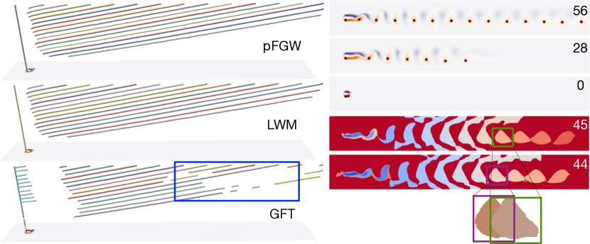
Figure 10: $\mathsf{Vortex\,Street}$. Left: comparing tracking results for pFGW, LWM, and GFT, respectively. Right top: snapshots of scalar fields at $t=0,28$, and $56$. Right bottom: merge-tree-based segmentation of the scalar fields at $t=44$ and $45$.

The tracking results for $\mathsf{Vortex\,Street}$ using pFGW, LWM and GFT are shown in Fig. 10 (left), in which there are 17, 17, and 27 trajectories, respectively. The results for pFGW and LWM are mostly identical, whereas the results from GFT show a number of oversegmentations and missing trajectories at later time steps (e.g., see the blue box). A few snapshots of the scalar field are shown in  Fig. 10 (right top), where local maxima are well aligned horizontally and moving rightward at an almost constant speed. This characteristic leads to a large number of straight-line trajectories, as shown in Fig. 10 (left). Meanwhile, a critical point remains stable in location to the left of the cylinder, whose trajectory is shown as a single straight line on the leftmost part of Fig. 10 for both pFGW and LWM.

6.4.2 Comparison with Previous Approaches

Our pFGW method and the LWM method perform similarly on $\mathsf{Vortex\,Street}$ in terms of reducing oversegmentations and mismatches. Meanwhile, similar to $\mathsf{Heated\,Cylinder}$ and $\mathsf{Unsteady\,Cylinder\,Flow}$, GFT typically introduces more oversegmentations in comparison with pFGW and LWM; in addition, certain trajectories may be missing due to insufficient feature overlaps between adjacent time steps. In Fig. 10 (right bottom), we show merge-tree-based segmentation of the scalar field at time steps $44$ and $45$. Here, the corresponding features at $t=44$ and $t=45$ move rapidly to the right (see the purple and green boxes, respectively). Although the features associated with these adjacent time steps are visually similar, their overlap is quite small based on their Jaccard index. Such insufficient feature overlaps appear to impact the tracking results significantly.

This observation motivates us to further compare pFGW, LWM, and GFT for subsampled data. We are interested in exploring the strengths and weaknesses of these methods when there are insufficient feature overlaps due to subsampling.

6.5 Ionization Front Dataset

We study the $\mathsf{Ionization\,Front}$ dataset by setting $\epsilon=10\%$, $\alpha=0.4$, and $L^{*}=0.02693$. A few snapshots of the scalar field at time steps $0,30,60$ and $90$ are shown in Fig. 11, as the instability progresses towards the right.

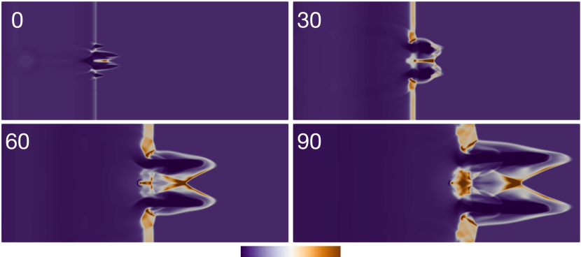
Figure 11: A few snapshots of $\mathsf{Ionization\,Front}$ dataset.

6.5.1 Tracking Results

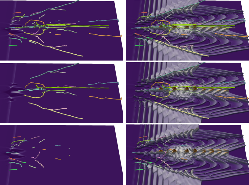
Figure 12: $\mathsf{Ionization\,Front}$. Left: pFGW trajectories are shown with the scalar field at time step $0$. Right: pFGW trajectories are visualized with the landscape of the time-varying scalar field. Top: all trajectories; middle: long-term trajectories; bottom: short-term trajectories.

We demonstrate our pFGW tracking results in Fig. 12 (left), where trajectories are shown with the scalar field at $t=0$. We then visualize these trajectories with the landscape of the time-varying scalar field in Fig. 12 (right), which is constructed by stacking the original scalar field at time steps $0$, $10$, $20$, …, $100$, and $110$. Such a landscape clearly shows the rightward propagation of the ionization front. The results shown in Fig. 12 (top) thus contain a number of trajectories that capture such a trend.

We further split these trajectories into two sets: trajectories that last longer than $29$ time steps (long-term trajectories) in Fig. 12 (middle), and those that last between $5$ and $29$ steps (short-term trajectories) in Fig. 12 (bottom). We ignore trajectories shorter than $5$ time steps as they do not capture the global trend of the data. A number of the long-term trajectories appear to follow the direction of the radiation waves, whereas some short-term trajectories capture local interactions among them.

6.5.2 Comparison with Previous Approaches

In terms of oversegmentations, pFGW, LWM, and GFT give rise to 51, 52, and 92 trajectories, respectively. pFGW produces slightly fewer trajectories than LWM, whereas GFT oversegments and produces the largest number of trajectories, see Fig. 13. In particular, GFT produces noticeably broken long-term trajectories, implying that it fails to track some major features consistently.

In terms of mismatches, trajectories from all three methods interpret the evolution of features in a similar way. However, pFGW produces the smallest (normalized) maximum distance of 0.02693, whereas LWM and GFT give rise to a (normalized) maximum distance of 0.03840.

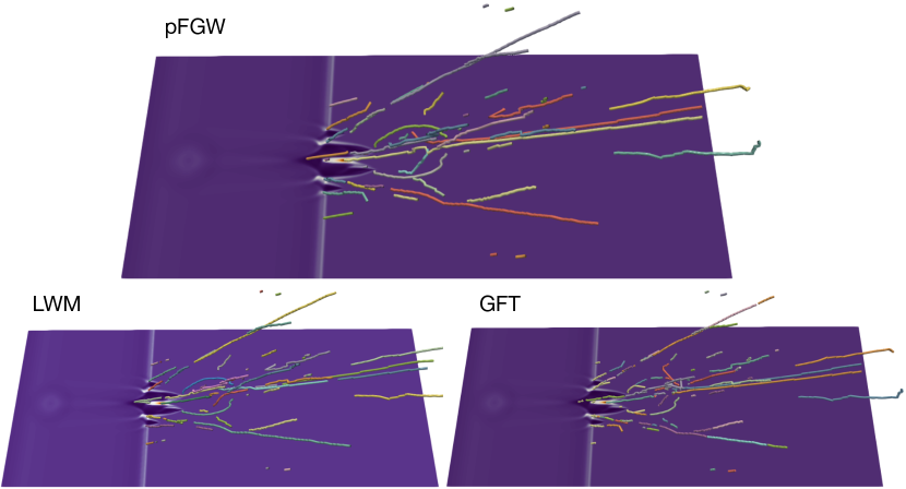
Figure 13: $\mathsf{Ionization\,Front}$. Comparing tracking results for pFGW, LWM, and GFT, respectively.

6.6 3D Isabel Dataset

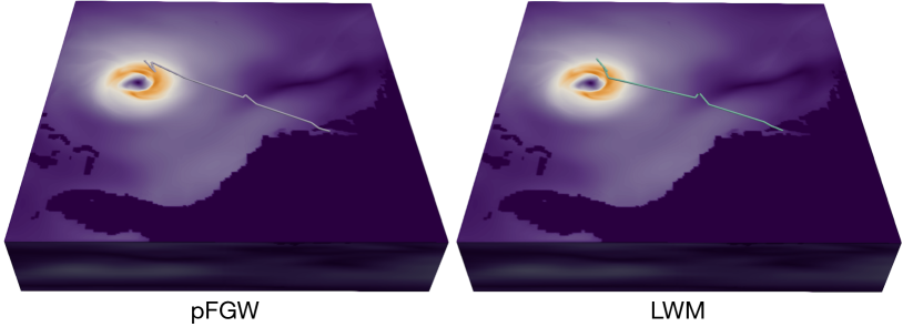
Figure 14: $\mathsf{Isabel}$. Tracking results for pFGW (left) and LWM (right).

Finally, for the 3D $\mathsf{Isabel}$ dataset, we apply both pFGW and LWM to track the trajectory of the global maximum, which highlights the movement of the main hurricane. This dataset contains a discrete set of time steps with large gaps; thus, it is not suitable for feature tracking based on region overlaps (such as GFT). As shown in Fig. 14, both pFGW and LWM successfully track the movement of the hurricane. These results highlight the robustness of topology-based feature tracking in 3D.

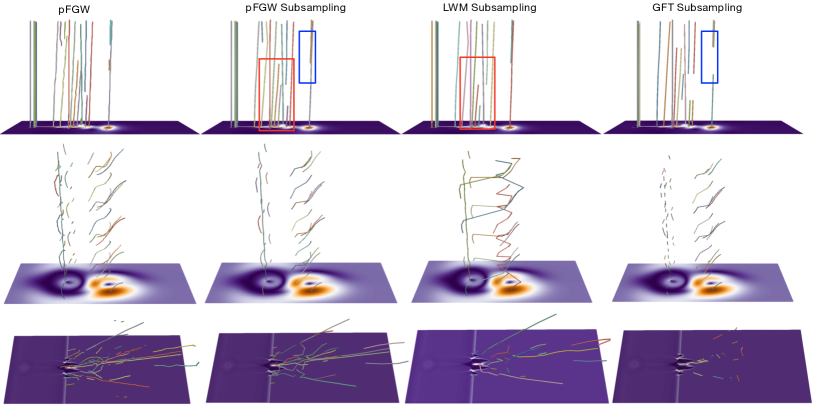
Figure 15: Tracking results of $\mathsf{Heated\,Cylinder}$ (top), $\mathsf{Unsteady\,Cylinder\,Flow}$ (middle), and $\mathsf{Ionization\,Front}$ (bottom) dataset under subsampling. From left to right: the original pFGW, pFGW, LWM, and GFT with subsampling, respectively.

6.7 Subsampling and Robust Tracking

For both the $\mathsf{Vortex\,Street}$ and $\mathsf{Isabel}$ datasets, we observe that topology-based feature tracking (such as pFGW and LWM) behaves better than geometry-based methods (such as GFT) when there are not sufficient region overlaps between adjacent time steps. In this section, we further examine the robustness of the three methods by subsampling time steps from previous datasets. We generate subsampled datasets by sampling a single instance for every $6$, $15$, and $10$ time steps for $\mathsf{Heated\,Cylinder}$, $\mathsf{Unsteady\,Cylinder\,Flow}$, and $\mathsf{Ionization\,Front}$ datasets, respectively.

6.7.1 Qualitative Comparisons

The tracking results for these subsampled datasets are shown in Fig. 15, using the original tracking pFGW results (first column) as a reference. We expect the tracked trajectories to be similar for a robust tracking method, with and without subsampling.

For the subsampled $\mathsf{Heated\,Cylinder}$ dataset in Fig. 15 (top), all three methods preserve the overall shape of trajectories, whereas pFGW demonstrates a slight advantage. In particular, some trajectories obtained by pFGW are missing by LWM (c.f., red boxes), whereas GFT produces oversegmentations (c.f., blue boxes).

For the subsampled $\mathsf{Unsteady\,Cylinder\,Flow}$ dataset in Fig. 15 (middle), LWM introduces obvious mismatches by matching geometrically distant critical points, whereas GFT creates a great number of broken trajectories on the left. In comparison, pFGW produces better tracking results without oversegmentations or mismatches.

For the subsampled $\mathsf{Ionization\,Front}$ dataset in Fig. 15 (bottom), all three methods show their limitations on tracking. LWM is able to preserve only a subset of long-term features and misses other features. It also produces a number of mismatches. For example, LWM incorrectly tracks the feature at the center of the domain to the outer boundary of the wave. GFT fails to preserve any major trajectories under subsampling. In comparison, pFGW is able to replicate major patterns of the trajectories, especially the long-term ones. However, we can also see some mismatches in its tracking results.

Based on these visualizations, pFGW is the best at preserving trajectories under subsampling while minimizing over-segmentations and mismatches. To evaluate these results quantitatively, we now discuss quantitative comparisons.

6.7.2 Quantitative Comparisons

We utilize the notion of the Jaccard index to study the similarity between two sets of trajectories. Let $a$ and $b$ denote a pair of trajectories, each of which contains a finite number of critical points sampled at discrete time steps. We define the overlap between $a$ and $b$ as their Jaccard index,

$$J(a,b)=\frac{|a\cap b|}{|a\cup b|}.$$

Let $A$ and $B$ be two sets of trajectories produced by two tracking methods, respectively. For each trajectory $a\in A$, define its matched trajectory $\pi(a)\in B$ such that $\pi(a)=\mathrm{argmax}_{b\in B}J(a,b).$ For any $a$, $\pi(a)$ may not be unique.

We then introduce two measures that quantify the similarity between $A$ and $B$:

$$S(A,B)=\frac{\sum_{a\in A}J(a,\pi(a))}{|A|}$$

$$S_{W}(A,B)=\frac{\sum_{a\in A}J(a,\pi(a))|a|}{\sum_{a\in A}|a|}$$

$S$ captures the average overlap of all trajectories in $A$ against their matched ones in $B$, whereas $S_{W}$ is a weighted version of $S$ considering the lengths of trajectories in the summations. $S$ and $S_{W}$ are not symmetric and have optimal values of $1$ when $A=B$.

In a subsampled dataset, a number of critical points may be missing from the original dataset. Let $A$ be the set of sub-trajectories from the original tracking results restricted to the subsampled time steps. Let $B$ be the set of trajectories obtained from the subsampled dataset. $S(A,B)$ and $S_{W}(A,B)$ describe how well a tracking algorithm preserves the trajectories against subsampling, whereas $S(B,A)$ and $S_{W}(B,A)$ indicate how well a tracking algorithm avoids mismatches in the subsampled dataset. In our experiment, we ignore (sub)trajectories of length $1$ as they are isolated critical points.

Dataset	Method	$S(A,B)$	$S(B,A)$	$S_{W}(A,B)$	$S_{W}(B,A)$
$\mathsf{Heated\,Cylinder}$	GFT	0.763	0.806	0.804	0.828
	LWM	0.642	0.714	0.663	0.672
	pFGW	0.821	0.782	0.827	0.806
$\mathsf{Unsteady\,Cylinder\,Flow}$	GFT	0.670	0.858	0.716	0.839
	LWM	0.229	0.403	0.307	0.446
	pFGW	0.907	0.990	0.957	0.991
$\mathsf{Ionization\,Front}$	GFT	0.314	0.452	0.228	0.419
	LWM	0.274	0.590	0.345	0.566
	pFGW	0.552	0.624	0.588	0.598

TABLE I: Similarity measures between a pair of tracking results with and without subsampling. For a fixed tracking method (pFGW, LWM, and GFT), $A$ denotes the subtrajectories from the original tracking results restricted to subsampled time steps. $B$ denotes the trajectories from the subsampled dataset.

The quantitive evaluation results are provided in Table I. pFGW is shown to have better performance than GFT and LWM in terms of capturing original trajectories under subsampling, for almost all cases. In particular, for the $\mathsf{Unsteady\,Cylinder\,Flow}$ and $\mathsf{Ionization\,Front}$ datasets, pFGW obtains significantly higher similarity measures than GFT and LWM. These results align well with our observations in Fig. 15 that pFGW is better at preserving trajectories and avoiding mismatches for subsampled datasets.

Drawbacks of GFT and LWM are also evident in Table I. For GFT, $S(A,B)$ and $S_{W}(A,B)$ over the $\mathsf{Unsteady\,Cylinder\,Flow}$ dataset are low because GFT fails to maintain continuity of trajectories on the left. For the $\mathsf{Ionization\,Front}$ dataset, GFT does not maintain long-term trajectories, leading to low similarity measures. For LWM, similarity measures are lowest for the $\mathsf{Unsteady\,Cylinder\,Flow}$ dataset due to significant mismatches in the tracking results. LWM maintains only a few long-term features for the $\mathsf{Ionization\,Front}$ dataset, leading to measures lower than those from pFGW.

To summarize, based on both qualitative and quantitative evaluations, GFT appears to lose its ability to track features when there are not sufficient time resolutions for geometry-based tracking, for instance, the subsampled $\mathsf{Ionization\,Front}$ dataset. Whereas LWM captures major features during tracking, it is not as robust as pFGW in tracking features for datasets with low time resolutions. For example, for the subsampled $\mathsf{Heated\,Cylinder}$ and $\mathsf{Ionization\,Front}$ datasets, LWM misses a large portion of the original trajectories. For the $\mathsf{Unsteady\,Cylinder\,Flow}$ dataset, LWM generates many obvious mismatches. Such drawbacks are also clearly reflected in the similarity measures. In comparison, our pFGW method performs quite well in robustly tracking features on datasets with low time resolutions.

6.7.3 Runtime Analysis

We perform runtime analysis for all three approaches (GFT, LWM, and pFGW) under the fine-tuned parameter configurations, as shown Table II. For the $\mathsf{Unsteady\,Cylinder\,Flow}$, $\mathsf{Vortex\,Street}$, $\mathsf{Ionization\,Front}$, and $\mathsf{Isabel}$ datasets, pFGW achieves a similar runtime with LWM. GFT is generally slower than the other two methods; it runs extremely slow on $\mathsf{Isabel}$, for which the runtime is not reported. pFGW is the slowest among the three for the $\mathsf{Heated\,Cylinder}$ dataset. Overall, all three methods take $\leq 0.01$ second to compute the feature matching between a pair of adjacent time steps. We do not include the runtime for merge tree generation as it is part of the data preprocessing. However, GFT is expected to spend more time on merge tree generation than LWM and pFGW, since it requires some extra information on merge tree segmentation.

Dataset	# of maxima	Time steps	Method	Total time (sec)	Avg. time
$\mathsf{Heated\,Cylinder}$	40	31	GFT	0.120	0.0040
			LWM	0.045	0.0015
			pFGW	0.146	0.0049
$\mathsf{Unsteady\,Cylinder\,Flow}$	16	499	GFT	1.049	0.0021
			LWM	0.325	0.0007
			pFGW	0.414	0.0008
$\mathsf{Vortex\,Street}$	30	59	GFT	0.148	0.0026
			LWM	0.095	0.0016
			pFGW	0.098	0.0017
$\mathsf{Ionization\,Front}$	40	123	GFT	0.577	0.0047
			LWM	0.333	0.0027
			pFGW	0.318	0.0026
$\mathsf{Isabel}$	14	12	GFT	NA	NA
			LWM	0.176	0.0160
			pFGW	0.012	0.0011

TABLE II: Runtime of feature tracking with GFT, LWM, and pFGW.

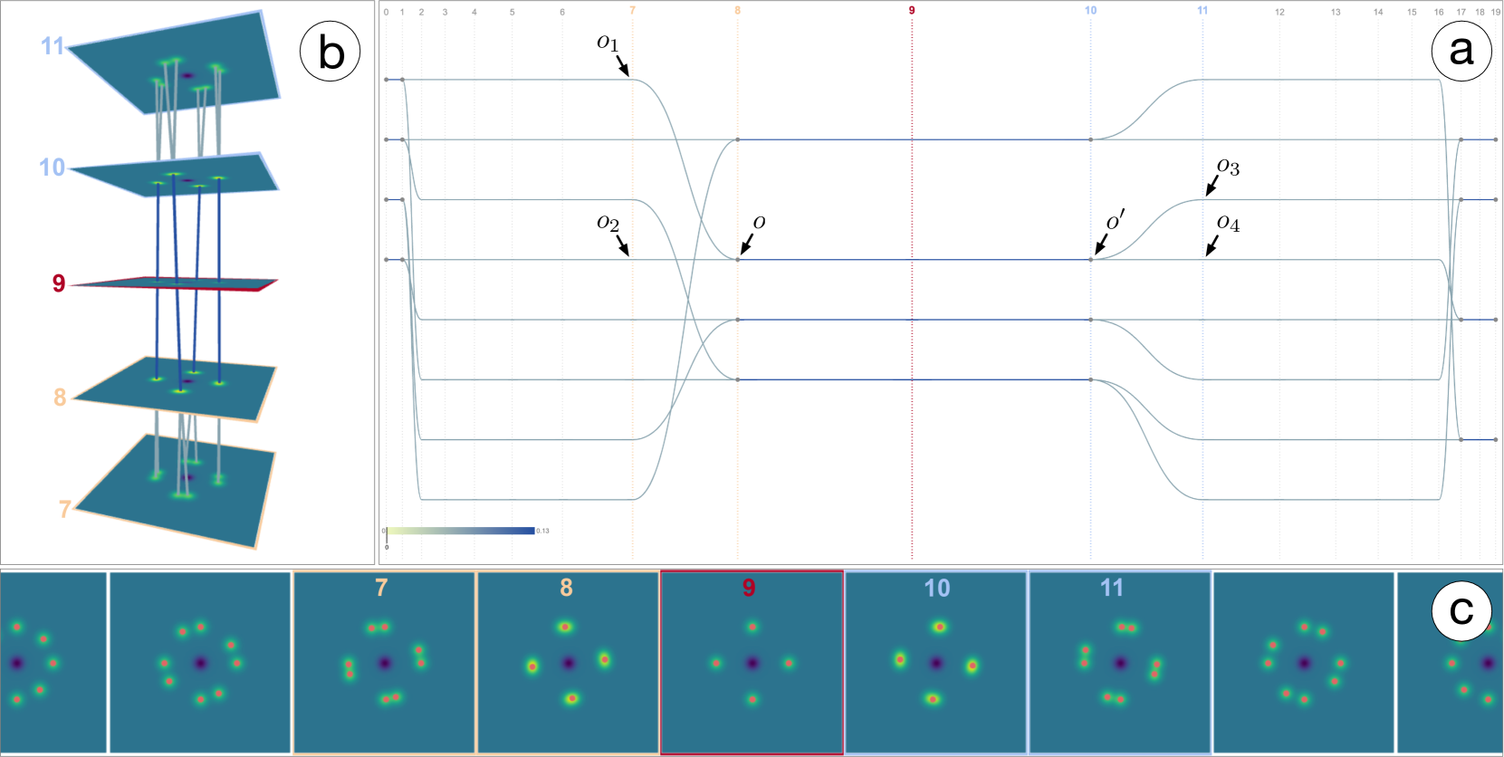
Figure 16: A visual demo of probabilistic feature tracking: the graph view (a), the track view (b), and the data view (c).

7 Probabilistic Tracking Graphs

A direct consequence of our pFGW method is that it enables richer representations of tracking graphs, referred to as probabilistic tracking graphs. The partial optimal transport provides a probabilistic coupling between features at adjacent time steps, which are then visualized by weighted tracks of these tracking graphs.

We provide a visual demo for probabilistic feature tracking for several 2D time-varying datasets. We illustrate its visual interface using a synthetic dataset. As shown in Fig. 16, the synthetic dataset is constructed as a mixture of nine Gaussian functions: one negative Gaussian function stays fixed at the center, eight Gaussian functions are positioned on a cycle, four of which remain stationary, whereas the other four move clockwise around the center. We focus on tracking the local maxima across time.

As shown in Fig. 16, the graph view (a) visualizes a tracking graph whose feature tracks are equipped with probabilistic tracking information. The track view (b) displays tracks across five consecutive time steps in 3D spacetime centered around the selected time step. The data view (c) presents the scalar fields at the same five time steps. With multiple views, users can explore the probabilistic feature tracking results from global and local perspectives.

The graph view (a) visualizes a tracking graph that captures the evolution of features across all time steps. Vertical time bars are positioned along the x-axis to represent time steps in increasing order, whereas tracks associated with individual features are laid out horizontally in a way that minimizes edge crossings. Nodes at the intersection of time bars and tracks represent features that appear, disappear, merge, or split. If feature $i$ from time $t$ is coupled with feature $j$ from time $t+1$ with a nonzero measure in the coupling matrix $C$, an edge is drawn between these two features in the tracking graph, whose color and opacity encodes the value of $C(i,j)$ as indicated in the color bar. $C(i,j)$ is a probability measure, where higher value implies a higher probability of matching feature $i$ with feature $j$. Users could filter the tracks in the tracking graphs by scrolling the color bar, in order to explore the tracking graphs at different probability thresholds.

In the tracking graph shown in Fig. 16 (a), when the four moving Gaussian functions coincide with the four stationary ones, their corresponding features merge together at time step $8$. Subsequently, these merged features split at time step $10$. The tracking graph depicts such events as probabilistic merges and splits. From time step $7$ to $8$, two features $o_{1}$ and $o_{2}$ merged into feature $o$ with the equal probability. Similarly, from time step $10$ to $11$, a single feature $o^{\prime}$ (that corresponds to $o$) splits into two ($o_{3}$ and $o_{4}$) with equal probability. These merging and splitting events are also encoded in the data view and the track view, see Fig. 16 (b) and (c). In this case, $o_{2}$ at time step $7$ corresponds to $o_{4}$ at time step $11$, $o$ at time step $8$ corresponds to $o^{\prime}$ at time step $10$; however, $o_{1}$ at time step $7$ does not match to $o_{3}$ at time step 11, since there are ambiguities in matching due to symmetry.

We now visually demonstrate the probabilistic tracking graph for the $\mathsf{Ionization\,Front}$ dataset. In the example shown in Fig. 17, we set the probability threshold at $0.023$ (main view) and $0.032$ (inserted view), respectively. To investigate the data of interest, users could select a specific time step $t$ by clicking its corresponding time bar, which updates views (a), (b), and (c). For the graph view (a), the select time bar is highlighted in red, with the previous two (at $t-2$, $t-1$) and subsequent two (at $t+1$, $t+2$) time bars colored in orange and blue, respectively. We smoothly adjust intervals between time steps based on the fisheye technique using animation, so that the focus area surrounding the selected time bar is magnified and the area away from the focus is compressed. For the track view (b), we render five scalar fields centered by the selected time step and highlight the tracks among them in a 3D spacetime, while supporting zooming and rotation. For the data view (c), we visualize the five 2D scalar fields side by side, where tracked features are highlighted in red.

Furthermore, our visual demo allows users to explore tracks associated with specific features. As illustrated in  Fig. 17, users can select a feature of interest (denoted by $o$), which sits at the intersection of four tracks $l_{1},l_{2},l_{3}$, and $l_{4}$; all of which are highlighted in red while maintaining their opacity. The track view (b) then displays these four tracks, whereas the data view (c) highlights the corresponding features (in magenta) along these tracks. In particular, two features, $o_{1}$ and $o_{2}$ at time step $69$ are coupled with feature $o$ at time step $70$ with relatively high probabilities. By increasing the tracking probability threshold, shown in the box insert, feature $o_{1}$ will stop its track at time step $69$, whereas features $o_{2}$ and $o$ remain matched with each other. Our visual demo showcases such uncertainty in tracking.

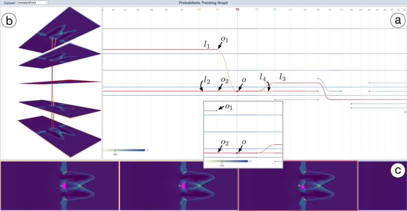
Figure 17: Selecting a particular feature $o$ to highlight relevant tracks (in red) and features (in magenta). The visual demo showcases uncertainty in tracking across different probability thresholds (see the box insert).

The visual demo is implemented using JavaScript for the front-end, where the tracking graphs are visualized with D3.js and the scalar fields are visualized using WebGL. The computational back-end is built with Python and Flask.

8 Conclusion

In this paper, we provide a flexible framework for tracking topological features in time-varying scalar fields. Our framework builds upon tools from topological data analysis (i.e., merge trees) and partial optimal transport. In particular, we model a merge tree as a measure network, and define a new partial fused Gromov-Wasserstein distance between a pair of merge trees. Such a distance gives rise to a partial matching between topological features in time-varying data, thus enabling flexible topology tracking for scientific simulations, as demonstrated by our extensive experiments.

On the other hand, our framework is not without limitations. First, we focus on feature tracking using merge trees, that is, we aim to preserve sublevel set relations between features (i.e., critical points) that are captured by merge trees. Other topological descriptors such as Reeb graphs and Morse complexes may capture different topological relations such as level set or gradient relations. We would like to explore topology tracking with partial optimal transport using other types of topological descriptors, which are left for future work. Second, we provide experimental justifications for parameter tuning; understanding parameter tuning from a theoretical standpoint seems elusive.

For future work, given the efficiency of our implementation, we would like to perform experiments involving datasets from large-scale simulations.

Appendix A A New Stability Theorem for GW Distance

In this section, we consider merge trees arising from functions on simplicial complexes and their associated measure network representations. Our goal is to prove the stability theorem, Theorem 2, which is a result in the tradition of topological data analysis (e.g., [63, 64, 65]). That is, we would like to show that a small change in the function data produces a small change in merge tree representations, as measured by the GW distance. We first remind the reader of technical details and notations before restating and proving the theorem.

Let $X$ be a finite, connected, geometric simplicial complex with a vertex set $V$. Let $f:X\to\mathbb{R}$ be a function obtained by starting with a function $f:V\to\mathbb{R}$ on the vertex set and extending linearly over higher dimensional simplices. These are the types of functions we deal with in our visualization pipelines. Let $T_{f}$ denote the merge tree for $f$, defined as a quotient space $T_{f}=X/\sim$. Of course, when dealing with merge trees computationally, they are represented by finite sets of points. A labeling of a merge tree $T$ is a map from a finite set $\pi:S\to T$, which is surjective onto the set of leaf nodes of $T$ [19]. Given a labeling, one can construct a least common ancestor matrix $W$, indexed over $S\times S$, where $W(s,t)$ is the height of the highest point along the unique geodesic path from $\pi(s)$ to $\pi(t)$ in $T$. It is shown in [19, Lemma 2.9] that a merge tree with labeling is uniquely encoded by its least common ancestor matrix. We will specifically choose a labeling of $T_{f}$ given by restricting the quotient map $X\to T_{f}$ to the finite vertex set $V$. In the following part of this section, let $\pi_{f}:V\to T_{f}$ denote this labeling map and let $W_{f}$ denote the least common ancestor matrix for this labeling.

Let $p$ be a probability distribution over the vertex set $V$. We will assume that $p$ is balanced, in the sense that for any $u,v,w\in V$, we have $p(u)\cdot p(v)\leq p(w)$; this property holds for the uniform distribution, for example. We then define the measure network representation of $T_{f}$ to be $G_{f}=(V,p,W_{f})$, with $W_{f}$ denoting the least common ancestor matrix, as defined above. We can also define a family of weighted norms on the space of functions $f:V\to\mathbb{R}$ by

$$\|f\|_{L^{q}(p)}:=\left(\sum_{v\in V}|f(v)|^{q}p(v)\right)^{1/q}.$$

We now restate Theorem 2.

Theorem 2. Let $f,g:X\to\mathbb{R}$ be functions defined as above and let $p$ be a balanced probability distribution. Then

$$d^{GW}_{q}(G_{f},G_{g})\leq\frac{1}{2}|V|^{2/q}\|f-g\|_{L^{q}(p)}.$$ (13)

The proof of the theorem will use Lemma 1.

Lemma 1.

The least common ancestor matrix $W_{f}$ of $f:X\to\mathbb{R}$ can be expressed as

$$W_{f}(v,w)=\min_{u_{1},u_{2},\ldots,u_{n}}\max_{u_{i}}f(u_{i}),$$

where the minimum is over paths $v=u_{1},u_{2},\ldots,u_{n}=w\in V$ where each pair of consecutive vertices is connected by an edge of $X$.

Proof.

We first show that

$$W_{f}(v,w)=\inf_{\gamma}\max_{t}f(\gamma(t)),$$

where the infimum is over continuous piecewise linear paths $\gamma:[0,1]\to X$ with $\gamma(0)=v$ and $\gamma(1)=w$. Indeed, any path $\gamma$ from $v$ to $w$ projects under the quotient map to a continuous path $\bar{\gamma}:[0,1]\to T_{f}$ from $\pi_{f}(v)$ to $\pi_{f}(w)$ ($\pi_{f}$ denoting the restriction of the quotient map $X\to T_{f}$ to the vertex set, as above) with property that $f(\gamma(t))=f(\bar{\gamma}(t))$ ($f$ denoting both the map $f:X\to\mathbb{R}$ and the induced map $f:T_{f}\to\mathbb{R}$, by abuse of notation). Then, we have

$$\inf_{\gamma}\max_{t}f(\gamma(t))=\inf_{\bar{\gamma}}\max_{t}f(\bar{\gamma}(t))\geq\inf_{\eta}\max_{t}f(\eta(t)),$$

where the latter infimum is over all continuous paths $\eta$ joining $\pi_{f}(v)$ to $\pi_{f}(w)$ in $T_{f}$. Since any such path will pass through the highest point along the unique geodesic path from $\pi_{f}(v)$ to $\pi_{f}(w)$, this infimum is equal to $W_{f}(v,w)$. Conversely, the geodesic path $\eta$ from $\pi(v)$ to $\pi(w)$ can be lifted to a piecewise linear path $\hat{\eta}$ joining $v$ to $w$ in $X$ with $f(\eta(t))=f(\hat{\eta}(t))$ for all $t$. It follows that

$$W_{f}(v,w)=\max_{t}f(\eta(t))=\max_{t}f(\hat{\eta}(t))\geq\inf_{\gamma}\max_{t}f(\gamma(t)).$$

To complete the proof, we claim that any piecewise linear path $\gamma$ joining $v$ to $w$ in $X$ can be replaced by a path that passes only through edges of $X$, without increasing the maximum height along the path. Indeed, this can be done constructively. First, break the image of the path into a sequence of concatenated paths $\gamma_{1},\gamma_{2},\ldots,\gamma_{n}$, where each $\gamma_{i}$ is contained in the relative interior of a simplex $X_{i}$ of $X$. By construction, $X_{i}$ will be either a face of $X_{i+1}$, or vice versa. Moreover, $X_{1}=v$ and $X_{n}=w$ (i.e., $\gamma_{1}$ and $\gamma_{n}$ are constant paths). To each $\gamma_{i}$, associate the vertex $u_{i}$ of $X_{i}$, which takes the lowest height. It follows that $u_{i}$ and $u_{i+1}$ are either equal or are connected by an edge for all $i$; we can ensure an edge path without repeats by simply removing repeated consecutive vertices. Since values of $f$ on $X$ are defined by linear interpolations of vertex values, $f(u_{i})$ is at most the max value of $f$ over $\gamma_{i}$. This completes the proof of the claim. It follows that

$$W_{f}(v,w)=\inf_{\gamma}\max_{t}f(\gamma(t))\geq\min_{u_{1},u_{2},\ldots,u_{n}}\max_{u_{i}}f(u_{i}).$$

Since any edge path defines, in particular, a piecewise linear path, this inequality is actually an equality and it completes the proof of the lemma. ∎

Proof.

(Proof of Theorem 2) The proof follows from a sequence of inequalities

$$2d^{GW}_{q}(G_{f},G_{g}) \leq\|W_{f}-W_{g}\|_{L^{q}(p\times p)}$$ (14)

$$\leq|V|^{2/q}\|(W_{f}-W_{g})\ast(p\times p)^{1/q}\|_{\infty}$$ (15)

$$\leq|V|^{2/q}\|(f-g)\ast p^{1/q}\|_{\infty}$$ (16)

$$\leq|V|^{2/q}\|f-g\|_{L^{q}(p)}.$$ (17)

We explain the notation and give a proof for each inequality below.

The right-hand side of Eq. (14) uses a weighted $L^{q}$ norm as defined above, for functions on $V\times V$. That is, for $F:V\times V\to\mathbb{R}$, we have

$$\|F\|_{L^{q}(p\times p)}=\left(\sum_{v,w\in V}|F(v,w)|^{q}p(v)p(w)\right)^{1/q}.$$

The inequality follows because the right-hand side is equal to the result of evaluating the $d^{GW}_{q}$ loss on the coupling induced by the identity map on $V$.

For $F:V\times V\to\mathbb{R}$, we define

$$\left(F\ast(p\times p)^{1/q}\right)(v,w):=F(v,w)\left(p(v)\cdot p(w)\right)^{1/q}.$$

Then, Eq. (15) follows from

$$\|W_{f}-W_{g}\|_{L^{q}(p\times p)} =\|(W_{f}-W_{g})\ast(p\times p)^{1/q}\|_{q}$$

$$\leq|V|^{2/q}\|(W_{f}-W_{g})\ast(p\times p)^{1/q}\|_{\infty},$$

where $\|\cdot\|_{q}$ denotes the standard $q$-norm (identifying the space of functions on $V\times V$ with $\mathbb{R}^{|V|^{2}}$) and the last inequality is a standard estimate on $q$-norms.

Similar to the above, for a function $h:V\to\mathbb{R}$, we define

$$\left(h\ast p^{1/q}\right)(v)=h(v)p(v)^{1/q}.$$

To establish Eq. (16), we refer to Lemma 1. Let $v,w\in V$ be arbitrary vertices and assume without loss of generality that $W_{f}(v,w)\geq W_{g}(v,w)$. We have

$$|W_{f}(v,w)-W_{g}(v,w)| =W_{f}(v,w)-W_{g}(v,w)$$

$$=\min_{u_{1},\ldots,u_{n}}\max_{u_{i}}f(u_{i})-\min_{x_{1},\ldots,x_{n}}\max_{x_{i}}g(x_{i}).$$

Let $x_{1}^{\ast},\ldots,x_{n}^{\ast}$ be a path realizing $W_{g}(v,w)$ and suppose that among these $x_{i}^{\ast}$’s, $f(x_{i}^{\ast})$ is maximized at $x_{k}^{\ast}$. Then

$$\min_{u_{1},\ldots,u_{n}}\max_{u_{i}}f(u_{i})\leq\max_{x_{i}^{\ast}}f(x_{i}^{\ast})\leq f(x_{k}^{\ast})$$

and

$$\min_{x_{1},\ldots,x_{n}}\max_{x_{i}}g(x_{i})=\max_{x_{i}^{\ast}}g(x_{i}^{\ast})\geq g(x_{k}^{\ast}),$$

hence

$$\min_{u_{1},\ldots,u_{n}}\max_{u_{i}}f(u_{i})-\min_{x_{1},\ldots,x_{n}}\max_{x_{i}}g(x_{i}) \leq\max_{x_{i}^{\ast}}f(x_{i}^{\ast})-\max_{x_{i}^{\ast}}g(x_{i}^{\ast})$$

$$\leq f(x_{k}^{\ast})-g(x_{k}^{\ast}).$$

Using the assumption that $p$ is balanced, we have

$$|(W_{f}-W_{g})(p\times p)^{1/q}(v,w)| \leq\left(f(x_{k}^{\ast})-g(x_{k}^{\ast})\right)\left(p(v)\cdot p(w)\right)^{1/q}$$

$$\leq\left(f(x_{k}^{\ast})-g(x_{k}^{\ast})\right)p(x_{k}^{\ast})^{1/q}$$

$$\leq\max_{u\in V}|(f(u)-g(u))p(u)^{1/q}|$$

$$=\|(f-g)\ast p^{1/q}\|_{\infty}.$$

Finally, Eq. (17) follows from a general bound on $q$-norms:

$$\|(f-g)\ast p^{1/q}\|_{\infty}\leq\|(f-g)\ast p^{1/q}\|_{q}=\|f-g\|_{L^{q}(p)}.$$

This equation completes the proof. ∎

Let us make some remarks about the result. First, if $p$ is chosen to be uniform, then the same proof gives an improved bound with a smaller power of $|V|$:

$$d^{GW}_{q}(G_{f},G_{g})\leq\frac{1}{2}|V|^{1/q}\|f-g\|_{L^{q}(p)}.$$

Next, the proof appears to be inefficient in that no optimization over couplings is used and that we pass through an $\infty$-norm rather than working directly with $q$-norms throughout. However, Eq. (13) is asymptotically tight up to a universal constant, as is shown by the following example. Let $V=\{v_{1},\ldots,v_{2n+1}\}$ and form $X$ by joining $v_{i}$ to $v_{i+1}$ by an edge for $i=1,\ldots,2n$. Define functions $f,g:V\to\mathbb{R}$ by setting $g(v_{i})=0$ for all $i$ and

$$f(v_{i})=\left\{\begin{array}[]{cl}0&i\neq n+1\\ 1&i=n+1.\end{array}\right.$$

Let $p$ be a probability distribution on nodes with

$$p(v_{i})=\left\{\begin{array}[]{cl}p_{0}&i\neq n+1\\ p_{1}&i=n+1,\end{array}\right.$$

where specific values of $p_{0}$ and $p_{1}$ are to be determined. Let $G_{f}(V,p,W_{f})$ and $G_{g}(V,p,W_{g})$ be the associated measure network representations of the merge trees.

Proposition 1.

With $f$, $g$, $G_{f}$ and $G_{g}$ as above, there exist choices of $p_{0}$ and $p_{1}$ such that $p$ is a balanced distribution and

$$\left(\frac{d_{q}^{GW}(G_{f},G_{q})}{\frac{1}{2}\|f-g\|_{L^{q}(p)}}\right)^{q}=C\cdot|V|^{2}+c_{|V|},$$

for a universal constant $C$, where $c_{|V|}$ represents a set of lower order terms in $|V|$.

Proof.

The coupling induced by the identity map is an optimal coupling of $G_{f}$ and $G_{g}$, hence

$$2d^{GW}_{q}(G_{f},G_{g}) =\|W_{f}-W_{g}\|_{L^{q}(p\times p)}=\|W_{f}\|_{L^{q}(p\times p)}$$

$$=\left(\sum_{v,w}W_{f}(v,w)^{q}p(v)p(w)\right)^{1/q}$$

$$=\left(2p_{0}^{2}n^{2}+p_{1}^{2}+4p_{0}p_{1}n\right)^{1/q},$$

where the last quantity is obtained by counting entries equal to one in the least common ancestor matrix $W_{f}$. On the other hand,

$$\|f-g\|_{L^{q}(p)} =\|f\|_{L^{q}(q)}$$

$$=\left(\sum_{v}f(v)^{q}p(v)\right)^{1/q}=p_{1}^{1/q}.$$

Since $|V|=2n+1$, we have

$$2p_{0}^{2}n^{2}+p_{1}^{2}+4p_{0}p_{1}n =\frac{1}{2}|V|^{2}p_{0}^{2}+(p_{0}^{2}+2p_{0}p_{1})|V|$$

$$\qquad\qquad\qquad+(\frac{1}{2}p_{0}^{2}+p_{1}^{2}+2p_{0}p_{1})$$

and it follows that

$$\left(\frac{d_{q}^{GW}(G_{f},G_{q})}{\frac{1}{2}\|f-g\|_{L^{q}(p)}}\right)^{q}=\frac{1}{2}|V|^{2}\frac{p_{0}^{2}}{p_{1}}+c_{|V|}.$$

The claim is proved (setting $C=\frac{1}{4}$) if we can choose $2p_{0}^{2}=p_{1}$ such that $2n\cdot p_{0}+p_{1}=1$ and $p_{0},p_{1}>0$, so that $p$ defines a valid probability density. Solving the system of equations with the given constraints, we get

$$p_{0}=-n+\sqrt{n^{2}+2}.$$

Moreover, we can check inequalities to show that the resulting probability density is balanced; the least obvious is $p_{1}^{2}\leq p_{0}$, which holds as soon as $n\geq 2$. ∎

Finally, we prove Corollary 1, which we restate here for convenience.

Corollary 1. Let $f,g:X\to\mathbb{R}$ be functions defined as above and let $p$ be a balanced probability distribution. Let $G_{f}$ (respectively, $G_{g}$) denote the representation of the merge tree $T_{f}$ ($T_{g}$) defined by the shortest path strategy. Then

$$d^{GW}_{q}(G_{f},G_{g})\leq\left(|V|^{2/q}+2\right)\|f-g\|_{L^{q}(p)}.$$

Proof.

Throughout this proof, we use $W_{f}$ and $W_{g}$ to represent least common ancestor matrices, and we use $D_{f}$ and $D_{g}$ to denote matrices of shortest path distances. Observe that for any $v,w\in V$ (the vertex set of $X$),

$$D_{f}(v,w)=2W_{f}(v,w)-f(v)-f(w).$$ (18)

Using notation from the proof of Theorem 2, it follows that

$$d^{GW}_{q}(G_{f},G_{g}) \leq\|D_{f}-D_{g}\|_{L^{q}(p\times p)}$$ (19)

$$=\|(2W_{f}-f-f)-(2W_{g}-g-g)\|_{L^{q}(p\times p)}$$ (20)

$$\leq 2\|W_{f}-W_{g}\|_{L^{q}(p\times p)}+2\|f-g\|_{L^{q}(p)}$$ (21)

$$\leq|V|^{2/q}\|f-g\|_{L^{q}(p)}+2\|f-g\|_{L^{q}(p)},$$ (22)

and the claim follows, once we justify the steps. Eq. (19) holds by the same reasoning as in the proof of Theorem 2, Eq. (20) is an application of Eq. (18), Eq. (21) is the triangle inequality for the $L^{q}$ norm, together with marginalizing out a copy of $p$ in the second term, and Eq. (22) follows from the proof of Theorem 2. ∎

Appendix B Experiments for the Stability Theorem

In this section, we present experiments that demonstrate our new stability theorem for GW distance in Sect. 5. First, we create a scalar field $f$ using a mixture of Gaussian functions. Second, we introduce different levels of noise $\iota$ to the scalar field, $f_{\iota}$. In particular, we add noise sampled uniformly from $\iota\in\{1\%,2\%,\dots,10\%\}$ of the range of $f$, see Fig. 18. For each instance of $\iota$, we generate $20$ random scalar fields.

We now compute the GW distance between the original scalar field $f$ and the noisy scalar fields $f_{\iota}$. We use SP and LCA strategies for encoding edge information and uniform strategy for encoding the node information (so that the probability distribution over the vertex set is always balanced).

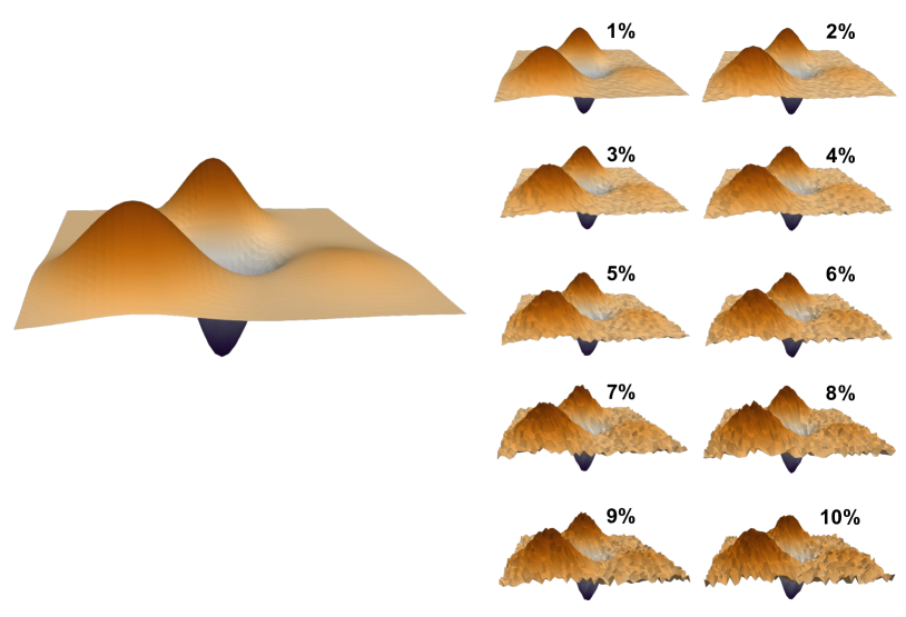
Figure 18: Left, a scalar field consists of multiple Gaussian functions. Right: ten datasets with different levels of noise.

As stated in Theorem 2, when the probability distribution over the vertex set is balanced, the upper bound for the GW distance using LCA strategy is $\frac{1}{2}|V|^{2/q}\|f-g\|_{L^{q}(p)}$; referred to as the loose bound. Furthermore, if the probability distribution on the node is uniform, there is a tighter upper bound of $\frac{1}{2}|V|^{1/q}\|f-g\|_{L^{q}(p)}$; referred to as the tight bound.

Our experimental results are shown in Fig. 19. In (a), we compute the GW distance between $f$ and $f_{\iota}$ across varying $\iota$ using the LCA strategy. For each fixed $\iota$, we compute the GW distances across $20$ instances and plot the corresponding box plot. We also plot the box plots associated with the tight and the loose bound, respectively. The line plots connect the mean values of these box plots. As shown in (a) and the zoomed-in view (b), the average GW distance (in blue) is upper bounded by the tight bound (in red), which is then upper bounded by the loose round (in yellow); thus validating Theorem 2.

On the other hand, as shown in Fig. 19(c), using the SP strategy, the bound for the GW distance $\left(|V|^{2/q}+2\right)\|f-g\|_{L^{q}(p)}$ is consistently higher than the GW distance itself in all our experiments; thus validating Corollary 1.

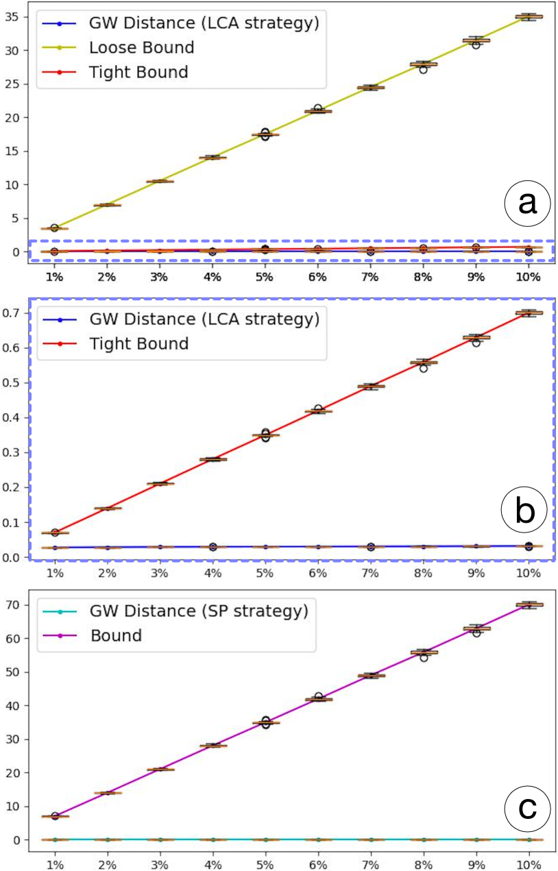
Figure 19: Box plots for the GW distance, the loose bound, and the tight bound under the LCA strategy (a-b), and the SP strategy (c).

Appendix C Parameter Tuning for GFT and LWM

We include details about parameter tuning for GFT and LWM described in Sect. 6 for reproducibility.

Parameters for GFT. $\lambda$ is a parameter used in GFT to balance the weight between region overlap size and histogram similarity. We follow the Github implementation (https://github.com/hsaikia/mtlib) to determine $\lambda$ using a binary search. Furthermore, GFT ignores matched feature pairs that have small region overlap and low histogram similarity (referred to as their combined similarity). We sort all matched pairs across all time steps based on their combined similarity. Keeping the top $5\%$ matched pairs is the optimal choice for all experiments in this paper.

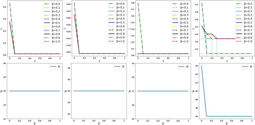
Figure 20: Parameter tuning of the LWM approach. From left to right: for the $\mathsf{Heated\,Cylinder}$, $\mathsf{Unsteady\,Cylinder\,Flow}$, $\mathsf{Vortex\,Street}$, and $\mathsf{Ionization\,Front}$ datasets, respectively. For each dataset, the top shows the maximum matched distances $L$ at each choice of $\beta$ as $\gamma$ changes. We use the elbow points to find the optimal value of $\gamma$ that produces the lowest $L$. The bottom shows the number of trajectories $N$ as $\beta$ changes with the optimal $\gamma$.

Parameters for LWM. There are five parameters introduced in LWM: $\alpha$, $\beta$, $\gamma_{x}$, $\gamma_{y}$, $\gamma_{z}$. $\alpha$ and $\beta$ are weights associated with the Wasserstein distance, whereas $\gamma_{x}$, $\gamma_{y}$, $\gamma_{z}$ are the weights for geometric distances between critical points on the corresponding axes. According to [25], when tracking local maxima, there are guidelines to follow: $\gamma_{x}=\gamma_{y}=\gamma_{z}=\gamma$, $\alpha=0.1\beta$. Hence, we use grid search to determine $\gamma$ and $\beta$.

Fig. 20 evaluates oversegmentations and mismatches during the parameter tuning process. We first apply a grid search for $\gamma$ and $\beta$: fixing $\beta$ for each curve, we compute the maximum matched distance with different values of $\gamma$, and find the optimal value of $\gamma$ at the elbow points. Using these optimal $\gamma$, we then compute the number of trajectories w.r.t. $\beta$.

Following this strategy for the $\mathsf{Heated\,Cylinder}$, $\mathsf{Unsteady\,Cylinder\,Flow}$, and $\mathsf{Vortex\,Street}$ datasets, we set $\gamma_{x}=\gamma_{y}=\gamma_{z}=\gamma=0.1$, $\alpha=0.1$, $\beta=1$. However, for $\mathsf{Ionization\,Front}$, we notice that when $\beta\geq 0.1$, the maximum matched distance is much higher than the one with $\beta=0$, which implies significant mismatches when $\beta\geq 0.1$. Therefore, regardless of the number of trajectories, we set $\gamma_{x}=\gamma_{y}=\gamma_{z}=0.1$, $\alpha=\beta=0$. It is noticeable that in LWM, $\beta$ does not affect much on feature tracking for these four test datasets (see Fig. 20 bottom). The geometric information appears to be the dominant factor in matching.

References

- [1] P.-T. Bremer, G. Weber, J. Tierny, V. Pascucci, M. Day, and J. Bell, “Interactive exploration and analysis of large-scale simulations using topology-based data segmentation,” IEEE Transactions on Visualization and Computer Graphics, vol. 17, no. 9, pp. 1307–1324, 2011.
- [2] W. Engelke, T. B. Masood, J. Beran, R. Caballero, and I. Hotz, “Topology-based feature design and tracking for multi-center cyclones,” in Topological Methods in Data Analysis and Visualization. Springer, 2021.
- [3] B. Friesen, A. Almgren, Z. Lukic, G. Weber, D. Morozov, V. Beckner, and M. Day, “In situ and in-transit analysis of cosmological simulations,” Computational Astrophysics and Cosmology, vol. 3, pp. 1–18, 2016.
- [4] C. Heine, H. Leitte, M. Hlawitschka, F. Iuricich, L. D. Floriani, G. Scheuermann, H. Hagen, and C. Garth, “A survey of topology-based methods in visualization,” Computer Graphics Forum, vol. 35, no. 3, pp. 643–667, 2016.
- [5] L. Yan, T. B. Masood, R. Sridharamurthy, F. Rasheed, V. Natarajan, I. Hotz, and B. Wang, “Scalar field comparison with topological descriptors: Properties and applications for scientific visualization,” Computer Graphics Forum, vol. 40, no. 3, pp. 599–633, 2021.
- [6] F. Mémoli, “On the use of Gromov-Hausdorff distances for shape comparison,” Eurographics Symposium on Point-Based Graphics, pp. 81–90, 2007.
- [7] ——, “Gromov-Wasserstein distances and the metric approach to object matching,” Foundations of Computational Mathematics, vol. 11, no. 4, pp. 417–487, 2011.
- [8] G. Peyré, M. Cuturi, and J. Solomon, “Gromov-Wasserstein averaging of kernel and distance matrices,” Proceedings of the 33rd International Conference on Machine Learning, PMLR, vol. 48, pp. 2664–2672, 2016.
- [9] S. Chowdhury and F. Mémoli, “The Gromov-Wasserstein distance between networks and stable network invariants,” Information and Inference: A Journal of the IMA, vol. 8, no. 4, pp. 757–787, 2019.
- [10] H. Xu, D. Luo, H. Zha, and L. C. Duke, “Gromov-Wasserstein learning for graph matching and node embedding,” in International conference on machine learning. PMLR, 2019, pp. 6932–6941.
- [11] H. Xu, D. Luo, and L. Carin, “Scalable Gromov-Wasserstein learning for graph partitioning and matching,” Advances in neural information processing systems, vol. 32, pp. 3052–3062, 2019.
- [12] S. Chowdhury and T. Needham, “Generalized spectral clustering via Gromov-Wasserstein learning,” in International Conference on Artificial Intelligence and Statistics. PMLR, 2021, pp. 712–720.
- [13] D. Alvarez-Melis and T. Jaakkola, “Gromov-Wasserstein alignment of word embedding spaces,” Proceedings of the Conference on Empirical Methods in Natural Language Processing, pp. 1881–1890, 2018.
- [14] P. Demetci, R. Santorella, B. Sandstede, W. S. Noble, and R. Singh, “Gromov-Wasserstein optimal transport to align single-cell multi-omics data,” BioRxiv preprint 2020.04.28.066787, 2020.
- [15] K.-T. Sturm, “The space of spaces: curvature bounds and gradient flows on the space of metric measure spaces,” arXiv preprint arXiv:1208.0434, 2012.
- [16] S. Chowdhury and T. Needham, “Gromov-Wasserstein averaging in a Riemannian framework,” Proceedings of the IEEE/CVF Conference on Computer Vision and Pattern Recognition Workshops, pp. 842–843, 2020.
- [17] M. Li, S. Palande, L. Yan, and B. Wang, “Sketching merge trees for scientific data visualization,” arXiv preprint arXiv:2101.03196, 2021.
- [18] J. Curry, H. Hang, W. Mio, T. Needham, and O. B. Okutan, “Decorated merge trees for persistent topology,” Journal of Applied and Computational Topology, pp. 1–58, 2022.
- [19] E. Gasparovic, E. Munch, S. Oudot, K. Turner, B. Wang, and Y. Wang, “Intrinsic interleaving distance for merge trees,” arXiv preprint arXiv:1908.00063, 2019.
- [20] F. Mémoli, A. Munk, Z. Wan, and C. Weitkamp, “The ultrametric Gromov-Wasserstein distance,” arXiv preprint arXiv:2101.05756, 2021.
- [21] T. Vayer, L. Chapel, R. Flamary, R. Tavenard, and N. Courty, “Fused Gromov-Wasserstein distance for structured objects,” Algorithms, vol. 13, no. 9, p. 212, 2020.
- [22] L. Chapel, M. Z. Alaya, and G. Gasso, “Partial optimal tranport with applications on positive-unlabeled learning,” Advances in Neural Information Processing Systems, vol. 33, pp. 2903–2913, 2020.
- [23] F. H. Post, B. Vrolijk, H. Hauser, R. S. Laramee, and H. Doleisch, “The state of the art in flow visualisation: Feature extraction and tracking,” Computer Graphics Forum, vol. 22, no. 4, pp. 775–792, 2003.
- [24] R. Bujack, L. Yan, I. Hotz, C. Garth, and B. Wang, “State of the art in time-dependent flow topology: Interpreting physical meaningfulness through mathematical properties,” Computer Graphics Forum, vol. 39, no. 3, pp. 811–835, 2020.
- [25] M. Soler, M. Plainchault, B. Conche, and J. Tierny, “Lifted Wasserstein matcher for fast and robust topology tracking,” in IEEE 8th Symposium on Large Data Analysis and Visualization (LDAV), Berlin, Germany, 2018, pp. 23–33.
- [26] M. Soler, M. Petitfrere, G. Darche, M. Plainchault, B. Conche, and J. Tierny, “Ranking viscous finger simulations to an acquired ground truth with topology-aware matchings,” in IEEE 9th Symposium on Large Data Analysis and Visualization, 2019, pp. 62–72.
- [27] M. Pont, J. Vidal, J. Delon, and J. Tierny, “Wasserstein distances, geodesics and barycenters of merge trees,” IEEE Transactions on Visualization and Computer Graphics, 2021.
- [28] L. Yan, T. B. Masood, F. Rasheed, I. Hotz, and B. Wang, “Geometry-aware merge tree comparisons for time-varying data with interleaving distances,” IEEE Transactions on Visualization and Computer Graphics (TVCG), 2022.
- [29] H. Saikia and T. Weinkauf, “Global feature tracking and similarity estimation in time-dependent scalar fields,” in Computer Graphics Forum, vol. 36, no. 3. Wiley Online Library, 2017, pp. 1–11.
- [30] ——, “Fast topology-based feature tracking using a directed acyclic graph,” in Topological Methods in Data Analysis and Visualization. Springer, 2017, pp. 155–169.
- [31] V. Divol and T. Lacombe, “Understanding the topology and the geometry of the space of persistence diagrams via optimal partial transport,” Journal of Applied and Computational Topology, vol. 5, no. 1, pp. 1–53, 2021.
- [32] J. Helman and L. Hesselink, “Representation and display of vector field topology in fluid flow data sets,” Computer, vol. 22, no. 8, pp. 27–36, 1989.
- [33] J. L. Helman and L. Hesselink, “Surface representations of two-and three-dimensional fluid flow topology,” in Proceedings of the 1st conference on Visualization’90. IEEE Computer Society Press, 1990, pp. 6–13.
- [34] T. Wischgoll, G. Scheuermann, and H. Hagen, “Tracking closed streamlines in time dependent planar flows,” in Proceedings of the Vision Modeling and Visualization Conference, 2001, pp. 447–454.
- [35] X. Tricoche, G. Scheuermann, and H. Hagen, “Topology-based visualization of time-dependent 2D vector fields,” in Symposium on Data Visualisation, 2001, pp. 117–126.
- [36] X. Tricoche, T. Wischgoll, G. Scheuermann, and H. Hagen, “Topology tracking for the visualization of time-dependent two-dimensional flows,” Computers & Graphics, vol. 26, no. 2, pp. 249–257, 2002.
- [37] H. Theisel and H.-P. Seidel, “Feature flow fields,” in Symposium on Data Visualisation, vol. 3, 2003, pp. 141–148.
- [38] T. Weinkauf, H. Theisel, A. Van Gelder, and A. Pang, “Stable Feature Flow Fields,” IEEE Transactions on Visualization and Computer Graphics, vol. 17, no. 6, pp. 770–780, Jun. 2011.
- [39] J. Reininghaus, J. Kasten, T. Weinkauf, and I. Hotz, “Efficient computation of combinatorial feature flow fields,” IEEE Transactions on Visualization and Computer Graphics, vol. 18, no. 9, pp. 1563–1573, 2012.
- [40] T. Vayer, N. Courty, R. Tavenard, and R. Flamary, “Optimal transport for structured data with application on graphs,” International Conference on Machine Learning, pp. 6275–6284, 2019.
- [41] R. Hendrikson, “Using Gromov-Wasserstein distance to explore sets of networks,” University of Tartu, Master Thesis, vol. 2, 2016.
- [42] T. Vayer, L. Chapel, R. Flamary, R. Tavenard, and N. Courty, “Fused Gromov-Wasserstein distance for structured objects,” Algorithms, vol. 13, no. 9, p. 212, 2020.
- [43] A. Figalli, “The optimal partial transport problem,” Archive for rational mechanics and analysis, vol. 195, no. 2, pp. 533–560, 2010.
- [44] J.-D. Benamou, G. Carlier, M. Cuturi, L. Nenna, and G. Peyré, “Iterative bregman projections for regularized transportation problems,” SIAM Journal on Scientific Computing, vol. 37, no. 2, pp. A1111–A1138, 2015.
- [45] L. Chizat, G. Peyré, B. Schmitzer, and F.-X. Vialard, “Scaling algorithms for unbalanced optimal transport problems,” Mathematics of Computation, vol. 87, no. 314, pp. 2563–2609, 2018.
- [46] A. Thual, H. Tran, T. Zemskova, N. Courty, R. Flamary, S. Dehaene, and B. Thirion, “Aligning individual brains with fused unbalanced Gromov-Wasserstein,” arXiv preprint arXiv:2206.09398, 2022.
- [47] M. Frank and P. Wolfe, “An algorithm for quadratic programming,” Naval Research Logistics Quarterly, vol. s, no. 1-2, pp. 95–110, 1956.
- [48] R. Flamary, N. Courty, A. Gramfort, M. Z. Alaya, A. Boisbunon, S. Chambon, L. Chapel, A. Corenflos, K. Fatras, N. Fournier et al., “Pot: Python optimal transport,” Journal of Machine Learning Research, vol. 22, no. 78, pp. 1–8, 2021.
- [49] J. Tierny, G. Favelier, J. A. Levine, C. Gueunet, and M. Michaux, “The Topology ToolKit,” IEEE Transactions on Visualization and Computer Graphics, vol. 24, no. 1, 2018.
- [50] H. Edelsbrunner, D. Letscher, and A. Zomorodian, “Topological persistence and simplification,” Discrete & Computational Geometry, vol. 28, 2002.
- [51] S. Popinet, “Free computational fluid dynamics,” ClusterWorld, vol. 2, no. 6, 2004. [Online]. Available: http://gfs.sf.net/
- [52] T. Günther, M. Gross, and H. Theisel, “Generic objective vortices for flow visualization,” ACM Transactions on Graphics, vol. 36, no. 4, pp. 141:1–141:11, 2017.
- [53] C. Jung, T. Tél, and E. Ziemniak, “Application of scattering chaos to particle transport in a hydrodynamical flow,” Chaos: An Interdisciplinary Journal of Nonlinear Science, vol. 3, no. 4, pp. 555–568, 1993.
- [54] “Computer graphics laboratory,” https://cgl.ethz.ch/research/visualization/data.php.
- [55] D. Whalen and M. L. Norman, “The IEEE SciVis Contest,” http://vis.computer.org/VisWeek2008/vis/contests.html, 2008.
- [56] ——, “Ionization front instabilities in primordial H II regions,” The Astrophysical Journal, vol. 673, no. 2, p. 664, 2008.
- [57] “Climate Data Gateway at NCAR,” https://www.earthsystemgrid.org/dataset/isabeldata.html.
- [58] S. Gerber, P.-T. Bremer, V. Pascucci, and R. Whitaker, “Visual exploration of high dimensional scalar functions,” IEEE Transactions on Visualization and Computer Graphics, vol. 16, pp. 1271–1280, 2010.
- [59] P.-T. Bremer, D. Maljovec, A. Saha, B. Wang, J. Gaffney, B. K. Spears, and V. Pascucci, “ND2AV: N-dimensional data analysis and visualization – analysis for the national ignition campaign,” Computing and Visualization in Science, vol. 17, no. 1, pp. 1–18, 2015.
- [60] “Global Feature Tracking,” https://github.com/hsaikia/mtlib.
- [61] J. P. Ahrens, B. Geveci, and C. C. Law, “Paraview: An end-user tool for large-data visualization,” in The Visualization Handbook, 2005.
- [62] W. Schroeder, K. Martin, and B. Lorensen, The Visualization Toolkit. Kitware, 2006.
- [63] D. Cohen-Steiner, H. Edelsbrunner, and J. Harer, “Stability of persistence diagrams,” Discrete & computational geometry, vol. 37, no. 1, pp. 103–120, 2007.
- [64] F. Chazal, D. Cohen-Steiner, L. J. Guibas, F. Mémoli, and S. Y. Oudot, “Gromov-Hausdorff stable signatures for shapes using persistence,” Computer Graphics Forum, vol. 28, no. 5, pp. 1393–1403, 2009.
- [65] P. Skraba and K. Turner, “Wasserstein stability for persistence diagrams,” arXiv preprint arXiv:2006.16824, 2020.