High-momentum oscillating tails of strongly interacting one-dimensional gases in a box

Abstract

We study the equilibrium momentum distribution of strongly interacting one-dimensional mixtures of particles at zero temperature in a box potential. We find that the magnitude of the $1/k^{4}$ tail of the momentum distribution is not only due to short-distance correlations, but also to the presence of the rigid walls, breaking the Tan relation relating this quantity to the adiabatic derivative of the energy with respect to the inverse of the interaction strength. The additional contribution is a finite-size effect that includes a $k$-independent and an oscillating part. This latter, surprisingly, encodes information on long-range spin correlations.

I Introduction

One-dimensional (1D) quantum systems of particles with contact interactions have been the playground for theoreticians for many years since they are exactly solvable with techniques such as Bethe ansatz LiebI ; LiebII ; Yang1967 ; Mcguire1964 ; Calabrese2007 and fermionization Girardeau1960 ; minguzzi2022strongly . Access to exact solutions was and is essential to improving our understanding of the role of quantum correlations in low dimensions Giamarchi_book ; giamarchi2011 . During the past decades, after being realized experimentally using different particle species, trapping geometries, and adjustable interactions Mistakidis2022 ; minguzzi2022strongly , the status of such systems has changed considerably. They have gone from being toy models to one of the paradigms for quantum simulators Gross2017 . In turn, they can even be considered as benchmarks for other, more complex, quantum simulators Shafer2020 . Among other examples, it is now possible to synthesize systems such as the Tonks-Girardeau (TG) gas of strongly interacting bosons Kinoshita1125 ; Parendes2004 or fermionic mixtures of $\kappa$ components with $SU(\kappa)$ interaction symmetry pagano_one-dimensional_2014 . The gas enters the TG regime when the ratio of the interaction energy to kinetic energy becomes very large and the probability of observing two particles in the same position becomes approximately zero.

Due to the diluteness of ultracold gases, atomic interactions can be well approximated by a zero-range potential and an important consequence of strong contact interactions is the universality of many equilibrium and thermodynamic quantities, most of them being summarized by the Tan relations tan_energetics_2008 ; tan_generalized_2008 ; tan_large_2008 ; BARTH20112544 ; Patu2017 . In one of them, the interplay between contact interactions and exchange symmetry between $N$ particles leads to the appearance of a universal algebraic behavior of the tail of the momentum distribution of the form $\mathcal{K}_{N}/k^{4}$ for momentum $\hbar k$ larger than any other typical momentum scale, such as the Fermi momentum $k_{\mathrm{F}}$.

$\mathcal{K}_{N}$ is usually identified with $\mathcal{C}_{N}$, Tan’s contact, which is proportional to $\partial E/\partial g^{-1}$, namely to $gE_{\mathrm{int}}$, the product between the interaction strength and the total interaction energy of the system lenard_momentum_1964 ; Minguzzi02 ; olshanii_short-distance_2003 . The equivalence $\mathcal{K_{N}}=\mathcal{C}_{N}$ holds at equilibrium for both homogeneous systems with periodic-boundary conditions and smoothly trapped systems, for any mixture of interacting particles, and any dimension tan_energetics_2008 ; tan_generalized_2008 ; tan_large_2008 ; BARTH20112544 .

The origin of the $1/k^{4}$ decay is the universal way the many-body wavefunction has to accommodate the contact interaction when two particles approach each other. For instance, antisymmetric exchanges neutralize the effects of contact interactions and do not contribute to $\mathcal{K}_{N}$, while symmetric exchanges induce in the many-body wavefunction, and thus in the one-body reduced density matrix (OBDM), a discontinuity of the derivative, a cusp, that contributes to the $\sim 1/k^{4}$ behavior of the momentum distribution tail Minguzzi02 ; olshanii_short-distance_2003 ; vignolo2013 . $\mathcal{K}_{N}$ is therefore sensitive to the exchange symmetry and can be used as observable for symmetry spectroscopy in quantum mixtures decamp_high-momentum_2016 ; decamp_strongly_2017 . This interplay of contact interactions and symmetry has repercussions on the spectrum of the finite interaction system volosniev_strongly_2014 ; decamp_high-momentum_2016 .

However, violations of the Tan relation have been pointed out in nonequilibrium scenarios, induced by impurities Cayla2023 , particle losses PhysRevLett.126.160603 , interaction quenches corson2016 ; rylands2023 , three-body effects colussi2020 , and at equilibrium for high temperatures derosi2023 . In this Letter, we show how the presence of a box confining potential also breaks down the Tan relation for 1D gases at equilibrium and zero temperature. We find that $\mathcal{K}_{N}$ not only has an average value larger than $\mathcal{C}_{N}$, but also, for strong interactions, develops oscillations [cf. Fig. 1], which are connected to the spin-coherence properties of the gas from one border of the box to the other.

Trapping atoms in optical-box potentials is becoming increasingly popular over the last years, and has led to important results in three-dimensional and two-dimensional gases navon2021box . Therefore, this work aims to guide future experiments using box potentials in one dimension.

We exemplify our findings using two canonical systems as spinless non interacting fermions and TG bosons (Sec. III), before generalizing them to arbitrary mixtures of quantum particles with infinite interactions (Sec. IV).

II General considerations

In the following, we briefly recall the definition of the momentum distribution and explain how its large-momenta tail is usually related to short-distance correlations in the system, thus to Tan’s contact olshanii_short-distance_2003 ; BARTH20112544 ; WernerCastin_ferm ; WernerCastin_bos . The momentum distribution $n(k)$, that is, the average density of particles with momentum $\hbar k$, can be expressed as the Fourier transform of the OBDM $\rho_{1}(x,y)$:

$$n(k)=\dfrac{1}{2\pi}\int\limits_{\mathcal{D}^{2}}dx\,dy\,\rho_{1}(x,y)e^{-ik(y-x)},$$ (1)

$$\!\!\!\!\rho_{1}(x,y)\!=\!N\!\!\!\!\!\!\int\limits_{\mathcal{D}^{N-1}}\!\!\!\!\!\!dx_{2}\cdots dx_{N}\,\Psi^{*}(x,x_{2},...,x_{N})\Psi(y,x_{2},...,x_{N}),$$ (2)

where $\Psi(x_{1},x_{2},...,x_{N})$ is the many-body wave function of $N$ particles, which, at this stage, can describe any kind of mixture. The integration domain $\mathcal{D}$ runs over the entire system and depends on the considered geometry.

In this Letter, we focus on the large-momenta tail of $n(k)$ given by

$$n(k)\underset{k\rightarrow\infty}{\simeq}\frac{\mathcal{K}_{N}}{k^{4}},$$ (3)

where the power-law decay derives from the type of singularity of $\rho_{1}(x,y)$ or $\Psi(x_{1},\dots,x_{N})$ and its weight $\mathcal{K}_{N}$ depends on the function slope in the vicinity of these singularities and on their number.

The origin of the $1/k^{4}$ tail can be understood by mathematical means. According to Watson’s lemma bleistein_asymptotic_1986 ; olshanii_short-distance_2003 , the asymptotics of the Fourier transform of functions which have a singularity of the type $f(z)=F(z)|z-z_{0}|^{\alpha}$, with $F(z)$ analytic, and $\alpha>-1$ and $\alpha\neq 0,2,4,\dots$ reads

$$\int\limits_{\mathcal{D}}dz~{}e^{-ikz}F(z)|z-z_{0}|^{\alpha}\!\!\underset{k\rightarrow\infty}{=}\!\!\mathcal{F}_{\alpha}\frac{e^{-ikz_{0}}F(z_{0})}{|k|^{\alpha+1}}+\mathcal{O}\left(\frac{1}{|k|^{\alpha+2}}\right),$$ (4)

where $\mathcal{F}_{\alpha}=2\cos[\pi(\alpha+1)/2]\Gamma(\alpha+1)$ and $\Gamma(\alpha)$ is the Gamma function. Therefore, by looking at Eqs. (1) and (2), the possible contributions to the $1/k^{4}$ tail of $n(k)$ could be seen as non-analytic terms of the form: (i) $|x-y|^{3}$ in $\rho_{1}(x,y)$ forrester_finite_2003 ; vignolo2013 or (ii) $|x-\bar{x}|$, with $\bar{x}\in\mathcal{D}$, in $\Psi(x,x_{2},..)$ Minguzzi02 ; olshanii_short-distance_2003 .

A pedagogical example of this behavior is provided by the TG gas for a smooth trapping potential. Its OBDM behaves as $|x-y|^{3}$ around $x\sim y$ and, consequently, $n(k)$ displays an algebraic tail forrester_finite_2003 . This differs from the case of free fermions and bosons in the same trap configuration, whose OBDMs are instead analytical in $\mathcal{D}$ and their momentum distributions do not have any algebraic tail note1 . This can be shown by expanding the OBDM for the TG gas, $\rho_{1}^{TG}$, in terms of the spinless fermions reduced density matrices $\rho_{1+j}^{F}$ with $j\geq 1$ lenard_onedimensional_1966 ; forrester_painleve_2003 , namely,

$$\begin{split}\rho_{1}^{\mathrm{TG}}(x,y)&=\rho_{1}^{\mathrm{F}}(x,y)+\sum_{j=1}^{N-1}\dfrac{(-2)^{j}}{j!}\int_{x}^{y}\!\!dx_{2}\dots dx_{1+j}\\ &\times\,\rho_{1+j}^{\mathrm{F}}(x,x_{2},\dots;y,x_{2},\dots),\end{split}$$ (5)

for $x<y$. For a smooth trapping potential, the only term that contributes to the $1/k^{4}$ algebraic decay of $n(k)$ is the first term of the expansion in Eq. (5), namely, $-2\int_{x}^{y}\!\!dx_{2}\rho_{2}^{F}(x,x_{2};y,x_{2})$ olshanii_short-distance_2003 . Indeed, by using Eq. (5) and introducing the change of coordinates $x_{r}=y-x$ and $X=(x+y)/2$, one has Fang09 ; vignolo2013

$$\begin{split}n^{\mathrm{TG}}(k)&\underset{k\rightarrow\infty}{\simeq}\dfrac{1}{2}\int\limits_{2\mathcal{D}}dx_{r}\,e^{-ikx_{r}}\dfrac{|x_{r}|^{3}}{6}\mathcal{C}_{N}^{\mathrm{TG}},\end{split}$$ (6)

where $1/k^{4}$ is given by applying Eq. (4) to the integral in $x_{r}$ and

$$\mathcal{C}_{N}^{\mathrm{TG}}\equiv\frac{2}{\pi}\int\limits_{\mathcal{D}}dX\,\lim_{\varepsilon\rightarrow 0}\dfrac{\rho_{2}^{\mathrm{F}}(X-\varepsilon,X;X+\varepsilon,X)}{\varepsilon^{2}}$$ (7)

is the Tan contact, which is equivalent to $\mathcal{K}_{N}$ in this case. Equation (7) enlightens the role of two-body correlations in $\mathcal{C}_{N}^{TG}$.

In the next sections, we will show how the presence of a box potential adds to the bulk term $\mathcal{C}_{N}^{\mathrm{TG}}$ an edge contribution. This is not only a trivial consequence of the cancellation of the wave function at the border, but also an interplay between rigid-border effects and coherence properties of the gas.

III One-component gases in a box

In order to investigate the effect of hard walls, we will discuss in this section two simple examples of 1D quantum gases at equilibrium in a box geometry ($x\in[-L/2,L/2]$) and at zero temperature note2 . We begin with a non-interacting Fermi gas whose momentum distribution does not have any algebraic tail in the homogeneous ring trap as well as in the presence of smoothly varying potentials. The second example will be the TG gas in a box, whose many-body wave function only differs from the one of spinless fermions by the particle-exchange symmetry.

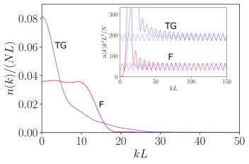
Figure 1: Normalized momentum distribution $n(k)/N$, in units of $1/L$, as a function of $kL$ for four spinless fermions (magenta) and four TG bosons (light violet). In the inset, the solid lines are the same $n(k)/N$ multiplied by $k^{4}$, in units of $L^{3}$, while the dashed lines correspond to the asymptotic analytical expressions given in Eqs. (9) and (12).

III.1 Spinless fermions

We now consider 1D spinless fermions trapped in a box of size $L$. In this case, the many-body wave function is simply the Slater determinant of $N$ lowest energy single-particle orbitals and the OBDM takes the form meckes_random_2019 ; Lacroix-a-chez-toine

$$\begin{split}\rho_{1}^{\mathrm{F}}(x,y)&=\dfrac{1}{2L}\left[\dfrac{\sin\left[(2N+1)\frac{\pi}{2L}(x-y)\right]}{\sin[\frac{\pi}{2L}(x-y)]}\right.\\ &\left.-\dfrac{\sin[(2N+1)\frac{\pi}{2L}(x+y+L)]}{\sin[\frac{\pi}{2L}(x+y+L)]}\right],\end{split}$$ (8)

with $|x|,|y|\leq L/2$. As explained in Sec. II, the calculation of the momentum distribution tail boils down to the investigation of nonanalyticities in the OBDM. In this case, they are only located at the edges, and the momentum distribution of the spinless Fermi gas develops an algebraic oscillating tail such that Bruyne2021 ; sup

$$\mathcal{K}^{\mathrm{F}}_{N}=\mathcal{B}_{N}+(-1)^{N+1}\mathcal{A}_{N}\cos\left(kL\right),$$ (9)

with $\mathcal{A}_{N}=N(N+1)\pi/L^{3}$ and $\mathcal{B}_{N}=(2N+1)\mathcal{A}_{N}/3$. The $k$-independent part $\mathcal{B}_{N}$ comes from contributions where $x$ and $y$ are close to the same edge. Roughly speaking, the effect of a hard wall in $L/2$ ($-L/2$) introduces a half cusp, with respect to the coordinates $x$ and $y$, of the form $|x-L/2|$ and $|y-L/2|$ ($|x+L/2|$ and $|y+L/2|$). Instead, the oscillating part is given by contributions of half cusps at opposite walls $(x\rightarrow\pm L/2,y\rightarrow\mp L/2)$. At first sight, it could be seen as an effect of diffraction by the box. However, its interpretation is more subtle and will become clearer when we will consider the case of a general mixture in Sec. IV. To support our conclusions, we have computed numerically the momentum distribution of a spinless Fermi gas of $N=4$ particles, and we have compared it with the asymptotic behavior given in Eq. (9) (see Fig. 1).

III.2 Tonks-Girardeau bosons

In order to calculate the asymptotic behavior of the momentum distribution for $N$ TG bosons trapped in a box, we start from the OBDM expressed as an expansion in terms of the spinless fermions $n$-body density matrices, as shown in Eq. (5). In the presence of smooth trapping potentials, we have already seen that only the first term of the series contributes to the contact. For the TG in a box, we can individuate three different contributions to the $1/k^{4}$ tail of the momentum distribution. The first contribution comes from $\rho_{1}^{\mathrm{F}}(x,y)$ and gives the terms in Eq. (9). This contribution is similar to the result found in Ref. PhysRevLett.126.160603 showing that the discrepancy between $\mathcal{K}_{N}$ and $\mathcal{C}_{N}$ in a Lieb-Liniger gas with losses is due to the contribution of the rapidities. The second contribution comes from $-2\int_{x}^{y}\!\!dx_{2}\rho_{2}^{\mathrm{F}}(x,x_{2};y,x_{2})$ and gives the usual Tan contact $\mathcal{C}_{N}$ [Eq. (7)], connected to the short-distance two-body correlations. For $N$ TG bosons in a box, we obtain

$$\mathcal{C}_{N}^{\mathrm{TG}}=\dfrac{N(N^{2}-1)(2N+1)}{3L^{3}}\pi=(N-1)\mathcal{B}_{N}.$$ (10)

Indeed, the two half cusps in $(+L/2,+L/2)$ and $(-L/2,-L/2)$ contributing to $\mathcal{B}_{N}$ have the same weight and scaling as the $(N-1)$ interparticles TG cusps of the bulk contribution $\mathcal{C}_{N}^{TG}$.

Remarkably, there is a third, nonlocal contribution entering the momentum distribution tail which can be derived by integrating all the higher-order fermionic density matrices of the second term in Eq. (5) over all the system. Indeed, it can be shown that sup

$$\begin{split}&\lim_{\begin{subarray}{c}x\rightarrow-\frac{L}{2}\\ y\rightarrow\frac{L}{2}\end{subarray}}\sum_{j=1}^{N-1}\dfrac{(-2)^{j}}{j!}\prod_{\ell=2}^{j+1}\int_{x}^{y}dx_{\ell}\,\rho_{1+j}^{\mathrm{F}}(x,x_{2},\dots;y,x_{2},\dots)\\ &=-2\rho_{1}^{\mathrm{F}}(x,y)|_{x\sim-\frac{L}{2},y\sim\frac{L}{2}},\end{split}$$ (11)

if $N$ is even and 0 otherwise. Such a term changes the sign of the oscillating part, with respect to the fermionic case if the number of particles is even. This means that for the TG gas, the sign of the oscillating part does not depend on the number of trapped bosons. Ultimately, we find that the asymptotic behavior of the momentum distribution for $N$ TG bosons in the box can be written as

$$\begin{split}\mathcal{K}^{\mathrm{TG}}_{N}&=\mathcal{C}_{N}^{\mathrm{TG}}+\mathcal{B}_{N}+\mathcal{A}_{N}\cos\left(kL\right)\\ &=\dfrac{N}{N-1}\mathcal{C}_{N}^{\mathrm{TG}}+\mathcal{A}_{N}\cos\left(kL\right).\end{split}$$ (12)

The average effect of the border ($\mathcal{B}_{N}$) is equivalent to the addition of a boson to the system. Moreover, it induces oscillations of the same amplitude as for a spinless Fermi gas, but with a phase that does not depend on the particle number parity. In order to elucidate this result, we plot in the inset of Fig. 1 the comparison between Eq. (12) and the numerical calculation of $\mathcal{K}_{N}$ for the case of $N=4$ particles. Notice that, in the thermodynamic limit, we recover the known result for the contact density $\mathcal{C}_{N}^{\mathrm{TG}}/L$ of a homogeneous TG gas with density $\mathlcal{n}=N/L$: $\lim_{N,L\rightarrow\infty}\mathcal{K}_{N}^{\mathrm{TG}}/L=\lim_{N,L\rightarrow\infty}\mathcal{C}_{N}^{\mathrm{TG}}/L=\frac{2}{3}\mathlcal{n}^{4}\pi$ Decamp2018 .

IV Mixtures in a box

We now generalize our results to strongly interacting bosonic and/or fermionic mixtures.

IV.1 Tonks-Girardeau limit for mixtures

We consider a 1D mixture of $N$ particles with $\kappa$ components and interacting via a two-body contact interaction. The Hamiltonian for this system is given by

$$\begin{split}\hat{H}&=\sum_{\sigma\sigma^{\prime}}^{\kappa}\sum_{i}^{N_{\sigma}}\left[-\frac{\hbar^{2}}{2m}\frac{\partial^{2}}{\partial x_{i,\sigma}^{2}}+g_{\sigma\sigma^{\prime}}\sum_{j>i}^{N_{\sigma^{\prime}}}\delta(x_{i,\sigma}-x_{j,\sigma^{\prime}})\right],\end{split}$$ (13)

where $i,j\in[1,N]$ and $\sigma,\sigma^{\prime}\in[1,\kappa]$ are the particle and spin indices, respectively, and $g_{\sigma,\sigma^{\prime}}$ is the inter- ($\sigma\neq\sigma^{\prime}$) or intra-species ($\sigma=\sigma^{\prime}$) interaction. Remarkably, the latter one is zero for identical fermions interacting via $s$-wave contact interactions. In the limit $g_{\sigma\sigma^{\prime}}\rightarrow+\infty$, for any $\sigma,\sigma^{\prime}$, the many-body wave function $\Psi$ vanishes whenever $x_{i}=x_{j}$. Thus, $\Psi$ can be written as follows volosniev_strongly_2014 ; deuretzbacher_quantum_2014 :

$$\Psi(X)=\sum_{P\in S_{N}}a_{P}\theta_{P}(X)\Psi_{A}(X),$$ (14)

where $X=(x_{1,\sigma_{1}},\dots,x_{N,\sigma_{N}})$ collects particle and spin indices, the index $P$ indicates a permutation inside the permutation group of $N$ elements, $S_{N}$, $\theta_{P}(X)$ is the generalized Heaviside function, which is equal to 1 in the coordinate sector $x_{P(1),\sigma_{P(1)}}<\dots<x_{P(N),\sigma_{P(N)}}$ and 0 elsewhere, and $\Psi_{A}$ is the wave function for $N$ spinless fermions. In particular, $\Psi_{A}$ is the Slater determinant built from the natural one-particle orbitals of the box.

Because of the statistics of identical particles, we can restrict the sum over $P$ in Eq. (14) to $N!/\prod_{\sigma}N_{\sigma}!$ independent elements instead of $N!$. These groups of sectors represent all the possible spin configurations and are usually called snippets Fang2011 ; volosniev_strongly_2014 . They constitute the proper basis for describing a multicomponent spin mixture and will be used throughout this section.

Moreover, in the strongly interacting limit, both for (i) the SU($\kappa$) case $1/g_{\sigma\sigma}=1/g_{\sigma\sigma^{\prime}}=1/g\ll 1$ and (ii) the broken symmetry one $1/g_{\sigma\sigma^{\prime}}=1/g\ll 1$ with $1/g_{\sigma\sigma}=0$ volosniev_engineering_2015 ; Aupetit2022 , the Hamiltonian in Eq. (13) can be mapped into the spin Hamiltonian

$$\hat{H}\underset{g\rightarrow\infty}{\rightarrow}E_{F}\mathbb{1}+H_{\mathrm{eff}}(J_{N}),$$ (15)

where $E_{F}$ is the Fermi energy related to the noninteracting system and $H_{\mathrm{eff}}=J_{N}(-(N-1)\mathbb{1}\pm\sum_{j}\hat{P}_{j,j+1})$, $\hat{P}_{j,j+1}$ being the permutation operator exchanging two interacting next-neighboring particles, and $J_{N}=(\hbar^{4}/m^{2})\alpha_{N}/g$ is the coupling constant with $\alpha_{N}=2E_{F}m/(\hbar^{2}L)$ $=\mathcal{B}_{N}\pi/2$ the nearest-neighbor exchange term deuretzbacher_momentum_2016 . Indeed, in the homogeneous system, $\hbar^{2}L\alpha_{N}/m$ is twice the total kinetic energy, which is connected to the slope of the cusps Barfknecht2021 ; Aupetit2022 .

For a multicomponent system, the OBDM can be written as $\rho_{1}(x,y)=\sum_{\sigma}N_{\sigma}\rho_{1,\sigma}(x,y)$ with

$$\rho_{1,\sigma}(x,y)=\sum_{i,j=1}^{N}c^{(i,j)}_{\sigma}\rho^{(i,j)}(x,y),$$ (16)

where $\rho^{(i,j)}(x,y)$ and $c^{(i,j)}_{\sigma}$ are the spatial and spin parts calculated on the sector $x_{1,\sigma_{1}}<\dots<x_{i-1,\sigma_{i-1}}<x<x_{i+1,\sigma_{i+1}}<\dots<x_{j,\sigma_{j}}<y<x_{j+1,\sigma_{j+1}}<\dots<x_{N,\sigma_{N}}$ deuretzbacher_momentum_2016 . In particular,

$$c_{\sigma}^{(i,j)}=\delta^{\sigma}_{\sigma_{i}}\sum_{P\in S_{N}}a_{P}a_{P_{i\rightarrow j}},$$ (17)

where $\delta^{\sigma}_{\sigma_{i}}$ selects only the sites with spin $\sigma_{i}=\sigma$ and $a_{P_{i\rightarrow j}}$ is the sector coefficient obtained by starting from the spin configuration labeled as $a_{P}$ and applying a cyclic permutation which takes the $i$-th element into the $j$-th position, and vice versa.

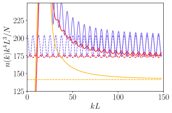
Figure 2: The solid lines stand for normalized momentum distribution $n(k)/N$ multiplied by $k^{4}$, in units of $L^{3}$, for the case of $2+2$ SU(2) bosons (i) in the ground state (violet, upper curve), (ii) in the first excited state (orange, central curve), and (ii) in the third excited state (yellow, lower curve). The dashed lines stand for the analytical expression of $\mathcal{K}_{N}^{\mathrm{mix}}/N$, Eq. (18), evaluated for cases (i), (ii), and (iii) (same color code).

IV.2 $\mathcal{K}_{N}$ for a mixture in the TG limit

All the elements required to compute the generalization of Eqs. (9) and (12) have been presented. For mixtures, the development is similar and is detailed in Ref. sup . The asymptotic behavior of the momentum distribution in the case of spin mixtures assumes the form

$$\begin{split}\mathcal{K}_{N}^{\mathrm{mix}}=&\mathcal{C}^{\mathrm{mix}}_{N}\!+\!\mathcal{B}_{N}\!+\!(-1)^{N\!+\!1}\!\!\mathcal{A}_{N}\sum_{\sigma}\frac{N_{\sigma}}{N}c_{\sigma}^{(1,N)}\!\!\cos(kL)\\ =&\dfrac{S\!+\!1}{N\!-\!1}\mathcal{C}_{N}^{\mathrm{TG}}\!+\!(-1)^{N\!+\!1}\!\!\mathcal{A}_{N}\sum_{\sigma}\frac{N_{\sigma}}{N}c_{\sigma}^{(1,N)}\!\!\cos\left(kL\right).\end{split}$$ (18)

The quantity

$$S=\sum_{P}\sum_{i=1}^{N-1}\left[\frac{1}{4}(a_{P}-a_{P_{i,i+1}})^{2}(1-\delta^{\sigma_{i+1}}_{\sigma_{i}})+\eta a_{P}a_{P_{i,i+1}}\delta^{\sigma_{i+1}}_{\sigma_{i}}\right]$$ (19)

takes into account the number of symmetric exchanges between particles Aupetit2022 and is proportional to the eigenvalue of the rescaled effective Hamiltonian $H^{\prime}_{\mathrm{eff}}=H_{\mathrm{eff}}/J_{N}$ [see Eq. (15)]. $P$ runs over the snippets and $\eta$ is equal to 1 for identical bosons and 0 otherwise. As expected, we can recover Eqs. (9) and (12) for the cases of spinless fermions and TG bosons, respectively. Indeed, it can be shown sup that for spinless fermions $S=0$ and $c_{\sigma}^{(1,N)}=1$, and for a TG gas $S=N-1$ and $\sum_{\sigma}\frac{N_{\sigma}}{N}c_{\sigma}^{(1,N)}=(-1)^{N+1}$ .

As for the one-component cases, the large-$k$ tail of $n(k)$ is not given solely by the Tan contact, but includes two additional terms. The first, the $k$-independent contribution $\mathcal{B}_{N}$, does not depend on the type of particles or mixture and counts such as an extra symmetric exchange in the mixture. The second, the oscillating part, is more intriguing, since the amplitude of the oscillations depends, remarkably, on long-distance spin correlations. Indeed, the only term of Eq. (16) that does not vanish in the limit $x\to-L/2$ and $y\rightarrow+L/2$ corresponds to the cyclic permutation $P_{1\to N}$ sup . Therefore, $c_{\sigma}^{(1,N)}$ can be interpreted as the one-body spin correlation through the whole system.

For the case of SU($\kappa$) bosonic or fermionic mixtures, the oscillation amplitude is maximal when the spin correlation is maximal, that is when the state of the system is equivalent to a single-component gas Aupetit2022 (meaning the ground state for bosonic and the most excited state for fermionic mixtures). Contrarily, as shown in Fig. 2, it vanishes for some particular cases where long-distance spin correlation is absent sup . The oscillation phase fluctuates by a factor $\pi$ depending, among other things, on the number of particles, for almost all states, except for the ground state of a SU($\kappa$) bosonic mixture sup .

V Concluding remarks

In conclusion, we have shown that the presence of a hard wall trapping potential breaks down the Tan relation connecting the $1/k^{4}$ decay of the momentum distribution of a 1D gas characterized by repulsive contact interactions to the adiabatic derivative of the energy with respect to the inverse of the interaction strength, even if the system is at equilibrium. In the strongly interacting limit, the presence of the two hard walls has a double effect. The first is rather trivial: it mimics the presence of an additional boson or impurity in the system. The second is more subtle: the tails develop oscillations whose amplitude depends on the nonlocal spin correlations over the whole system size. The sign of this contribution depends generally on the number of particles, except for the ground state of a bosonic $SU(\kappa)$ mixture. This can be of particular interest for experiments. In ultracold gases, the momentum distribution can be measured by switching off the trapping potential and imaging the cloud after a ballistic expansion Parendes2004 ; pagano_one-dimensional_2014 , and these measurements are obtained by averaging over system realizations where the number of particles fluctuates shot to shot. Therefore, the observation of oscillating tails in $n(k)$ of $SU(\kappa)$ bosonic mixtures could be used to determine whether the system is mainly cooled down in its ground state or not. Indeed, only in the first case the oscillation amplitude will be not vanishing. Let us remark that identifying the exact populated state might be experimentally difficult since the spectrum of a strongly interacting mixture is characterized by the presence of a large number of states very close in energy to the ground state deuretzbacher_exact_2008 ; decamp_high-momentum_2016 .

Finally, our study can be extended to finite temperatures and different dimensions, and out-of-equilibrium scenarios, such as spin-mixing dynamics pecci2022 .

References

- (1) E. H. Lieb and W. Liniger, Phys. Rev. 130, 1605 (1963).
- (2) E. H. Lieb, Phys. Rev. 130, 1616 (1963).
- (3) C. N. Yang, Phys. Rev. Lett. 19, 1312 (1967).
- (4) J. B. McGuire, J. Math. Phys. 5, 622 (1964).
- (5) P. Calabrese and J.-S. Caux, Phys. Rev. Lett. 98, 150403 (2007).
- (6) M. Girardeau, J. Math. Phys. 1, 516 (1960).
- (7) A. Minguzzi and P. Vignolo, AVS Quantum Sci. 4, 027102 (2022).
- (8) T. Giamarchi, Quantum Physics in One Dimension, (Clarendon Press, Oxford, 2003).
- (9) M. A. Cazalilla, R. Citro, T. Giamarchi, E. Orignac, and M. Rigol, Rev. Mod. Phys. 83, 1405 (2011).
- (10) S. Mistakidis, A. Volosniev, R. Barfknecht, T. Fogarty, T. Busch, A. Foerster, P. Schmelcher, and N. Zinner, arXiv:2202.11071 (2022).
- (11) C. Gross and I. Bloch, Science 357, 995 (2017).
- (12) F. Schäfer, T. Fukuhara, S. Sugawa, Y. Takasu, and Y. Takahashi, Nat. Rev. Phys. 2, 411 (2020).
- (13) T. Kinoshita, T. Wenger, and D. S. Weiss, Science 305, 1125 (2004).
- (14) B. Paredes, A. Widera, V. Murg, O. Mandel, S. Fölling, I. Cirac, G. V. Shlyapnikov, T. W. Hänsch, and I. Bloch, Nature 429, 277 (2004).
- (15) G. Pagano, M. Mancini, G. Cappellini, P. Lombardi, F. Schäfer, H. Hu, X.-J. Liu, J. Catani, C. Sias, M. Inguscio, and L. Fallani, Nat. Phys. 10, 198 (2014).
- (16) S. Tan, Ann. Phys. 323, 2952 (2008).
- (17) S. Tan, Ann. Phys. 323, 2987 (2008).
- (18) S. Tan, Ann. Phys. 323, 2971 (2008).
- (19) M. Barth and W. Zwerger, Ann. Phys. 326, 2544 (2011).
- (20) O.I. Pâţu and A. Klümper, Phys. Rev. A 96, 063612 (2017).
- (21) A. Lenard, J. Math. Phys. 5, 930 (1964).
- (22) A. Minguzzi, P. Vignolo, and M. Tosi, Phys. Lett. A 294, 222 (2002).
- (23) M. Olshanii and V. Dunjko, Phys. Rev. Lett. 91, 090401 (2003).
- (24) P. Vignolo and A. Minguzzi, Phys. Rev. Lett. 110, 020403 (2013).
- (25) J. Decamp, J. Jünemann, M. Albert, M. Rizzi, A. Minguzzi, and P. Vignolo, Phys. Rev. A 94, 053614 (2016).
- (26) J. Decamp, J. Jünemann, M. Albert, M. Rizzi, A. Minguzzi, and P. Vignolo, New J. Phys. 19, 125001 (2017).
- (27) A. G. Volosniev, D. V. Fedorov, A. S. Jensen, M. Valiente, and N. T. Zinner, Nat. Commun. 5, 5300 (2014).
- (28) H. Cayla, P. Massignan, T. Giamarchi, A. Aspect, C. I. Westbrook, and D. Clément, Phys. Rev. Lett. 130, 153401 (2023).
- (29) I. Bouchoule and J. Dubail, Phys. Rev. Lett. 126, 160603 (2021).
- (30) J. P. Corson, and J. L. Bohn, Phys. Rev. A 94, 023604 (2016).
- (31) C. Rylands, P. Calabrese, and B. Bertini, Phys. Rev. Lett. 130, 023001 (2023).
- (32) V. E. Colussi, H. Kurkjian, M. Van Regemortel, S. Musolino, J. van de Kraats, M. Wouters, and S. J. J. M. F. Kokkelmans, Phys. Rev. A 102, 063314 (2020).
- (33) G. D. Rosi, G. E. Astrakharchik, M. Olshanii, and J. Boronat, arXiv:2302.03509 (2023).
- (34) N. Navon, R. P. Smith, and Z. Hadzibabic, Nature Physics 17, 1334 (2021).
- (35) F. Werner and Y. Castin, Phys. Rev. A 86, 013626 (2012).
- (36) F. Werner and Y. Castin, Phys. Rev. A 86, 053633 (2012).
- (37) N. Bleistein and R. A. Handelsman, Asymptotic Expansions of Integrals, (Dover Publications, New York, 1986).
- (38) P. J. Forrester, N. E. Frankel, T. M. Garoni, and N. S. Witte, Phys. Rev. A 67, 043607 (2003).
- (39) For example, in a homogeneous trap ring, the momentum distribution for free fermions is a step Fermi function and for free bosons is a Dirac .
- (40) A. Lenard, J. Math. Phys. 7, 1268 (1966).
- (41) P. Forrester, N. Frankel, T. Garoni, and N. Witte, Commun. Math. Phys. 238, 257 (2003).
- (42) B. Y. Fang, P. Vignolo, C. Miniatura, and A. Minguzzi, Phys. Rev. A 79, 023623 (2009).
- (43) Here, we consider an ideal box, but in the experiments, the walls of the trap could have a local curvature . In that case, our results would be valid for .
- (44) E. S. Meckes, The Random Matrix Theory of the Classical Compact Groups, (Cambridge University Press, Cambridge, 2019).
- (45) B. Lacroix-A-Chez-Toine, P. Le Doussal, S. N. Majumdar and G. Schehr, J. Stat. Mech. 123103 (2018).
- (46) B. De Bruyne, D. S. Dean, P. Le Doussal, S. N. Majumdar, and G. Schehr, Phys. Rev. A 104, 013314 (2021).
- (47) See Supplemental Material for additional details about the derivations of the equations in Secs. III-IV.
- (48) J. Decamp, M. Albert, and P. Vignolo, Phys. Rev. A 97, 033611 (2018).
- (49) F. Deuretzbacher, D. Becker, J. Bjerlin, S. M. Reimann, and L. Santos, Phys. Rev. A 90, 013611 (2014).
- (50) B. Fang, P. Vignolo, M. Gattobigio, C. Miniatura, and A. Minguzzi, Phys. Rev. A 84, 023626 (2011).
- (51) A. G. Volosniev, D. Petrosyan, M. Valiente, D. V. Fedorov, A. S. Jensen, and N. T. Zinner, Phys. Rev. A 91, 023620 (2015).
- (52) G. Aupetit-Diallo, G. Pecci, C. Pignol, F. Hébert, A. Minguzzi, M. Albert, and P. Vignolo, Phys. Rev. A 106, 033312 (2022).
- (53) F. Deuretzbacher, D. Becker, and L. Santos, Phys. Rev. A 94, 023606 (2016).
- (54) R. Barfknecht, A. Foerster, N. Zinner, and A. G. Volosniev, Commun. Phys. 4, 252 (2021).
- (55) F. Deuretzbacher, K. Fredenhagen, D. Becker, K. Bongs, K. Sengstock, and D. Pfannkuche, Phys. Rev. Lett. 100, 160405 (2008).
- (56) G. Pecci, P. Vignolo, and A. Minguzzi, Phys. Rev. A 105, L051303 (2022).