Recent developments in warm inflation

Abstract

Warm inflation, its different particle physics model implementations and the implications of dissipative particle production for its cosmology are reviewed. First, we briefly present the background dynamics of warm inflation and contrast it with the cold inflation picture. An exposition of the space of parameters for different well-motivated potentials, which are ruled out, or severely constrained in the cold inflation scenario, but not necessarily in warm inflation, is provided. Next, the quantum field theory aspects in realizing explicit microscopic models for warm inflation are given. This includes the derivation of dissipation coefficients relevant in warm inflation for different particle field theory models. The dynamics of cosmological perturbations in warm inflation are then described. The general expression for the curvature scalar power spectrum is shown. We then discuss in details the relevant regimes of warm inflation, the weak and strong dissipative regimes. We also discuss the results predicted in these regimes of warm inflation and how they are confronted with the observational data. We explain how the dissipative dynamics in warm inflation can address several long-standing issues related to (post-) inflationary cosmology. This includes recent discussions concerning the so-called swampland criteria and how warm inflation can belong to the landscape of string theory.

I Introduction

Among the different proposals that attempted to implement consistent inflationary dynamics within an explicit quantum field theory realization, the warm inflation (WI) paradigm Berera:1995wh ; Berera:1995ie ; Berera:1998px is one of the most attractive. Warm inflation explores the fact that the inflationary dynamics is inherently a multifield problem, since the vacuum energy that drives inflation eventually must be converted to radiation, which generally is comprised of a variety of particle species. Thus, WI model realizations explore those associated dissipative processes to realize radiation production concurrently with the inflationary expansion. This is the opposite of the more usual scenario of cold (supercooled) inflation (CI) Guth:1980zm ; Sato:1981ds ; Albrecht:1982wi ; Linde:1981mu ; Linde:1983gd , where a separated period of radiation production after the end of inflation (graceful exit) is required.

From a model building perspective, the recent developments have aimed at overcoming some of the important issues found in earlier particle physics realizations of warm inflation. In order to be able to sustain a nearly-thermal bath during WI, a sufficiently strong dissipation is typically required, such that some of the energy density in the inflaton can be converted to radiation. For this to happen, earlier particle physics realizations of WI required large field multiplicities BasteroGil:2009ec ; Bartrum:2013fia . These large field multiplicities can be difficult to be generated in simple models while keeping perturbativity and unitarity in these models Bastero-Gil:2012akf (see, however, for natural realizations in the context of brane models Bastero-Gil:2011zxb , or in extra-dimensional models with a Kaluza-Klein tower Matsuda:2012kc ). One other difficulty in WI model building is to properly control both quantum and thermal corrections to the inflaton such as not to spoil the flatness of its potential, which could otherwise prevent inflation to happen. Earlier models for WI have made use, for instance, of both supersymmetry and heavy intermediate fields coupled to the inflaton for this purpose Berera:2002sp ; Berera:2008ar . More recent implementations of WI have focused, instead, in using symmetry properties such as to be able to efficiently control the corrections to the inflaton potential Bastero-Gil:2016qru ; Bastero-Gil:2019gao ; Berghaus:2019whh . Finally, from an effective field theory point of view, WI constructions that can be able to achieve strong dissipative regimes have been shown to display quite appealing features. For example, already in some of the first studies in WI Berera:1999ws ; Berera:2004vm it has been claimed that WI in the strong dissipative regime can also prevent super-Planckian field excursions for the inflaton, thus making WI potentially attractive in terms of an effective field theory consistent with an UV-complete realization in terms of quantum gravity Das:2018hqy ; Motaharfar:2018zyb ; Das:2018rpg ; Das:2019hto ; Kamali:2019xnt ; Brandenberger:2020oav ; Das:2020xmh ; Berera:2019zdd ; Berera:2020dvn ; Kamali:2019hgv ; Kamali:2019wdh ; Berera:2020iyn ; Kamali:2018ylz ; Kamali:2021gkl . Finally, the dissipative effects in WI can lower the energy scale of inflation and, as a result of this, the tensor-to-scalar ratio can be decreased with respect to what it would be in CI for the same type of primordial inflaton potential. This makes several primordial inflaton potential models that would otherwise be and had been discarded in CI, to be in line with the CMB observations in the context of WI Benetti:2016jhf . The above are just a few examples of recent developments in WI and which have been attracting increasingly interest in this intriguing alternative picture of inflation. In this paper we review some of these major developments achieved in the area in the recent years.

This paper is divided as follows. In Section II, we start by briefly reviewing the WI background dynamics and contrasting it to the CI picture. We discuss how a supplementary friction term in the Klein-Gordon equation is able to bring about a richer dynamics for WI. The smooth connection of the end of WI with the radiation dominated regime is discussed. We show that there are several different possibilities for graceful exit depending on the form of the inflaton potential, the dissipation coefficient and whether being in the weak or strong dissipative regimes. In Section III, we describe the necessary tools for calculating dissipation coefficients in the context of non-equilibrium quantum field theory and which are applied to WI. Some of the most recent microscopic realizations of WI are discussed and the respective derivation of the dissipation coefficients for these models is outlined. In Section IV, we discuss the cosmological perturbation theory for WI. Several important issues are discussed and the general derivation of the scalar of curvature power spectrum in WI is given. The bispectrum and non-Gaussianities in WI are also discussed. In Section V, we discuss the observational constraints and other applications of the WI dissipative dynamics. It is shown how the dissipative particle production addresses/alleviates some of the long-outstanding problems in cosmology, e.g., related to the inflationary and post-inflationary phases and which CI cannot directly answer. In Section V, we also discuss the connections which WI recently made with the so-called swampland criteria. We start by briefly reviewing the motivation behind the swampland conjectures Obied:2018sgi ; Ooguri:2018wrx ; Kinney:2018nny ; Bedroya:2019snp ; Agrawal:2018own ; Bedroya:2019tba . We discuss why the dynamics of WI allows it to satisfy the swampland conjectures. Given the constraints imposed by the swampland conjectures, we find under which conditions WI is able to simultaneously satisfy the swampland conjectures and the implications and the implications of this for building inflationary models in string theory in the context of WI. An overview of different WI implementations and applications, including in the context of noncanonical models, is also given. Finally, in Section VI, we give our concluding remarks.

II Background Dynamics of WI

A WI regime is typically realized when the inflaton field is able to dissipate its energy into other light degrees of freedom with a rate that is faster than the Hubble expansion. Thus, the produced particles have enough time to thermalize and become radiation. During this time, where the inflaton is decaying into the radiation particles and that can subsequently thermalize, one can then model their contributions as simply a radiation fluid with $\rho_{r}=\pi^{2}g_{*}T^{4}/30$, with $\rho_{r}$, $T$ and $g_{*}$ being the radiation energy density, the temperature and the effective number of relativistic degrees of freedom of the produced particles. Hence, the total energy density of the universe in the WI scenario contains both the inflaton field and a primordial radiation energy density, i.e., $\rho=\rho_{\phi}+\rho_{r}$, where $\rho_{\phi}$ is the inflaton field energy density. Energy conservation then demands that the energy lost by the inflaton field must be gained by the radiation fluid. Therefore, the evolution equations can be obtained from the conservation of the energy-momentum tensor $T^{\mu\nu}$ Bastero-Gil:2011rva ,

$$\nabla_{\mu}T^{\mu\nu}=0.$$ (1)

We work in the spatially flat Friedmann-Lemaître-Robertson-Walker (FLRW) metric, $ds^{2}=-dt^{2}+a(t)^{2}\delta_{ij}dx^{i}dx^{j}$, where $a(t)$ is the scale factor. Hence, Eq. (1) leads to a set of continuity equations for each component of the cosmological fluid,

$$\dot{\rho}_{\alpha}+3H(\rho_{\alpha}+p_{\alpha})=Q_{\alpha},$$ (2)

where a dot here means a derivative with respect to the cosmic time $t$, with $\rho_{\alpha}$ and $p_{\alpha}$ being the energy density and pressure for each fluid component $\alpha$, respectively, and $H\equiv\dot{a}/a=\sqrt{\rho/3}/M_{\rm Pl}$ is the Hubble expansion rate. Here, $M_{\rm Pl}=(8\pi G)^{-\frac{1}{2}}\simeq 2.44\times 10^{18}$ GeV is the reduced Planck mass and $G$ is Newton’s gravitational constant. Moreover, $Q_{\alpha}$ in Eq. (2) is a the source term, which describes the energy conversion between the species $\alpha$ accounted in the theory. The conservation of energy assures that $\sum_{\alpha}Q_{\alpha}=0$. Therefore, the conversion of the inflaton energy density into radiation energy density in the WI scenario is, hence, described by the following set of equations BasteroGil:2009ec

$$\dot{\rho}_{\phi}+3H(\rho_{\phi}+p_{\phi}) =-\Upsilon(\rho_{\phi}+p_{\phi}),$$ (3)

$$\dot{\rho}_{r}+3H(\rho_{r}+p_{r}) =\Upsilon(\rho_{\phi}+p_{\phi}),$$ (4)

where $\Upsilon$ is the dissipation coefficient, which can generally be a function of the inflaton field $\phi$ and temperature $T$ and whose functional form depends on how WI is being described in terms of the microscopic physics Bastero-Gil:2012akf ; Bartrum:2013fia ; Bastero-Gil:2016qru ; Berghaus:2019whh ; Bastero-Gil:2019gao . Considering the energy density and pressure for a standard canonical inflaton field, i.e., $\rho_{\phi}=\dot{\phi}^{2}/2+V(\phi)$ and $p_{\phi}=\dot{\phi}^{2}/2-V(\phi)$, with $p_{r}=\rho_{r}/3$, Eqs. (3) and (4) reduce to

$$\ddot{\phi}+(3H+\Upsilon)\dot{\phi}+V_{\phi} =0,$$ (5)

$$\dot{\rho}_{r}+4H\rho_{r}=\Upsilon\dot{\phi}^{2},$$ (6)

where $V_{\phi}$ is the derivative of the inflaton potential with respect to $\phi$. Although inflation happens when the energy density is dominated by the inflaton field potential $V$, i.e., $\rho_{r},\ \dot{\phi}^{2}/2\ll V$, such that the radiation energy density is sub-dominant, even so the produced radiation energy density can still satisfy $\rho^{1/4}_{r}>H$. Assuming thermalization, this condition then translates into $T>H$, which is usually considered as a condition for WI to happen. This condition is easy to understand. Since the typical mass for the inflaton field during inflation is $m_{\phi}\simeq H$, hence, when $T>H$, thermal fluctuations of the inflaton field will become important. Looking at Eq. (5), one can immediately see that dissipative particle production effects manifest as an extra friction term in the equation of motion for the inflaton. Therefore, radiation will not be necessarily redshifted during inflation, because it can be continuously fed by the inflaton through dissipation. As a consequence, this can result in a sustainable quasi-stationary thermal bath during the inflationary dynamics. Such radiation production also results in entropy production. The entropy density $s$ is related to the radiation energy density by $Ts=4\rho_{r}/3$, i.e., it is related to the temperature as $s={2\pi^{2}g_{*}}T^{3}/45$, where we have considered a thermalized radiation bath as it is typically the case in the WI scenario. Then, Eq. (6) can be rewritten in terms of the entropy density as follows Moss:2008yb

$$T(\dot{s}+3Hs)=\Upsilon\dot{\phi}^{2}.$$ (7)

With the inflaton’s potential dominating, an inflationary phase sets in. Thus, to solve Eqs. (5) and (6), one can use the so-called slow-roll approximation, which consists in dropping the leading derivative term in each equation, i.e., $\ddot{\phi}\ll 3H\dot{\phi},V_{\phi}$ and $\dot{\rho}_{r}\ll 4H\rho_{r},\Upsilon\dot{\phi}^{2}$. Hence, the slow-roll equations read as follows,

$$3H(1+Q)\dot{\phi}+V_{\phi} \simeq 0,$$ (8)

$$\rho_{r} \simeq\frac{3}{4}Q\dot{\phi}^{2},$$ (9)

and $H\simeq\sqrt{V/3}/M_{\rm Pl}$. In Eqs. (8) and (9), we have introduced $Q$,

$$Q=\frac{\Upsilon}{3H},$$ (10)

which defines the dissipation ratio in WI and it measures the strength of the dissipative particle production effects in comparison to the spacetime expansion. There are two different regimes in WI that can be defined depending on the value of the dissipation ratio $Q$. The weak dissipative regime is when $Q<1$. In this regime, dissipation is not expected to modify significantly the background dynamics. Hence, in this case the background dynamics is similar as in CI. However, as we will see in the Section IV, thermal fluctuations of the radiation energy density can still strongly affect the field fluctuations, and also the primordial spectrum of perturbations as long as $T>H$. The other regime of WI is the strong dissipative regime, $Q>1$. In this case, dissipation strongly modifies both the background dynamics and the primordial fluctuations. Note that $Q$ is not necessarily constant. In fact, it can increase or decrease depending on the form of dissipation coefficient and inflaton potential. Therefore, there is also a possibility that a model can start in the weak dissipative regime, but later on to transit into the strong dissipative regime, or vice versa. Let us discuss in more details these different possibilities that can appear in WI and how dissipation ultimately affects the dynamics.

From the slow-roll equations, one can express the Hubble slow-roll parameter $\epsilon_{H}$ in terms of the so-called potential slow-roll parameter $\epsilon_{V}$ as follows,

$$\epsilon_{H}\equiv-\frac{\dot{H}}{H^{2}}\simeq\frac{1}{2}M_{\rm Pl}^{-2}(1+Q)\frac{\dot{\phi}^{2}}{H^{2}}\simeq\frac{\epsilon_{V}}{(1+Q)},$$ (11)

where $\epsilon_{V}={M^{2}_{\rm Pl}}(V_{\phi}/V)^{2}/2$. To reach the second equality in Eq. (11), we have used the second Friedmann equation, i.e., $-2M^{2}_{\rm Pl}\dot{H}=\rho+P$, together with Eq. (9) and then used Eq. (8) to reach the last equality. One can realize from Eq. (11) that inflation will end when $\epsilon_{H}\simeq 1$ or, equivalently, when $\epsilon_{V}\simeq 1+Q$. Moreover, looking at the last equality in Eq. (11), one can immediately see that the equality between the Hubble slow-roll and the potential slow-roll parameters as observed in the CI, $\epsilon_{H}\simeq\epsilon_{V}$, does not hold in the WI scenario. In the CI scenario, the inflationary phase occurs when the Hubble slow-roll parameter is smaller than unity, i.e., $\epsilon_{H}\ll 1$, which means that the potential slow-roll parameter should also be smaller than unity. However, in the WI scenario, the inflationary phase occurs even when the potential slow-roll parameter is bigger than one (or even much bigger than one), provided that the dissipation ratio is large enough. This in particular alleviates the need for very flat potentials, as far as the background dynamics is concerned. Moreover, defining the number of e-folding as $N=\ln a$, i.e., $dN=Hdt=(H/\dot{\phi})d\phi$, which measures the expansion of the universe, one can see from the last two expressions in Eq. (11) that $d\phi/dN=M_{\rm Pl}\sqrt{2\epsilon_{V}}/(1+Q)$, which means that the inflaton field excursion can be much smaller in the WI scenario than in comparison to the CI scenario for the same variation of $\epsilon_{H}$. In fact, the inflaton field excursion in WI can be sub-Planckian even for very steep potentials. We will discuss later in section V how such novel background dynamics will allow WI to reside in the landscape of the string theory.

When using the slow-roll approximation in Eqs. (3) and (4), one should carefully consider its consistency. This consistency check can be performed, for instance, using a linear stability analysis to determine under which conditions the system remains close to the slow-roll solution for many Hubble times Moss:2008yb . Through this procedure, one finds that the sufficient conditions for the slow-roll approximation to hold are

$$\epsilon_{V},\eta_{V},\beta_{V}\ll 1+Q,\ \ \ \ \ \ \ 0<b\ll\frac{Q}{1+Q},\ \ \ \ \ \ \ \ \ |c|<4,$$ (12)

where we have defined the additional quantities $\eta_{V}=M^{2}_{\rm Pl}V_{\phi\phi}/V$, $\beta_{V}=M^{2}_{\rm Pl}V_{\phi}\Upsilon_{\phi}/V\Upsilon$, $b=TV_{\phi T}/V_{\phi}$ and $c=T\Upsilon_{T}/\Upsilon$. The condition on the parameter $b$ states that the thermal correction to the inflaton potential should be small, while the condition on the parameter $c$ reflects the fact that radiation has to be produced at a rate larger than the red-shift due to the expansion of the universe. Therefore, slow-roll WI occurs when all conditions in Eq. (12), together with $T>H$, are satisfied. However, one may wonder that the condition for WI to happen is in conflict with the conditions for the slow-roll approximation. Using Eq. (9) and given that $T>H$ during inflation, one finds that

$$\frac{\dot{\phi}^{2}/2}{V(\phi)}>\frac{\pi^{2}g_{*}}{135}Q^{-1}\frac{H^{2}}{M^{2}_{\rm Pl}}.$$ (13)

Since $H\ll M_{\rm Pl}$ in most inflationary models, one can find that the WI scenario is consistent with the slow-roll approximation even for the weak dissipation regime, $Q<1$. Moreover, one shall further show that the radiation energy density will never exceed the potential energy in the slow-roll regime, thus guaranteeing a period of accelerated expansion. To this end, one can calculate the radiation energy density to potential energy density ratio as follows,

$$\frac{\rho_{r}}{V}\simeq\frac{1}{2}\frac{\epsilon_{V}}{1+Q}\frac{Q}{1+Q}.$$ (14)

During inflation $\epsilon_{H}\ll 1$, meaning that $\rho_{r}\ll V$, even for a large dissipation ratio, while at the end of inflation $\epsilon_{H}\simeq 1$, i.e., $\epsilon_{V}\simeq 1+Q$, implying that $\rho_{r}\simeq V$, if the strong dissipation regime can be achieved. Therefore, radiation will not be diluted and can even become dominant at the end of inflation. As a consequence, the universe can smoothly enter into the radiation dominated epoch without the need of a separate reheating phase as required in the CI scenario. Therefore, there is a possibility that even potentials without a minimum can also be embedded into a WI scenario without any difficulty. In other words, those inflationary potentials without minimum, which have attracted considerable attention due to recently proposed swampland conjectures inspired from string theory, usually result in an ever-lasting inflationary phase in the CI scenario and they require another mechanism for termination of inflation. However, inflation will end due to dissipative particle production in the WI scenario even if the inflaton potential has no minimum. Hence, larger classes of inflationary potentials can be embedded into the WI scenario due to its richer dynamics in comparison to the CI case.

Having discussed under which conditions a slow-roll WI dynamics can be consistently achieved, one next consistency check is to investigate under which conditions the inflationary phase can end in this context. Looking at Eq. (11), one can see that there are several possibilities for graceful exit in the WI scenario. The end of WI depends on the form of the potential, on the dissipation coefficient and whether the regime of weak or strong dissipation has been achieved. In other words, the inflationary phase can continue as long as $\epsilon_{V}<1+Q$ and it will end when $\epsilon_{V}\simeq 1+Q$. Although in the CI scenario inflation ends when $\epsilon_{V}$ increases during inflation, in the WI scenario, there is a possibility that even potentials with constant and decreasing $\epsilon_{V}$ have graceful exit, since $Q$ is also a dynamical parameter. In fact, depending on the evolution of $\epsilon_{V}$ and $Q$ there are generally three possibilities for graceful exit in WI scenario. First, if $\epsilon_{V}$ increases, inflation ends when $Q$ decreases, remains constant or not increases faster than $\epsilon_{V}$. In fact, potentials such as the monomial potentials, hilltop potentials, natural inflation potential and the Starobinsky potential, which have a graceful exit in CI scenario, also have graceful exit in WI depending on the form of dissipation coefficient. Second, if $\epsilon_{V}$ is constant, in the exponential type of potentials, inflation ends only when $Q$ is a decreasing function. Third, if $\epsilon_{V}\gg 1$ and it is a decreasing function, inflation ends when $Q$ decreases much faster than $\epsilon_{V}$ and cross $\epsilon_{V}$ before it become less than unity. Although the last possibility exists in the WI scenario, it is very challenging from a model building point of view and these models usually do not end as in the case of the CI scenario (see Ref. Das:2020lut for more details). All of the aforementioned possibilities can be summarized in terms of the Hubble slow-roll parameter in such a way that inflation ends when $\epsilon_{H}$ increases with the number of e-folding. Therefore, taking the derivative with respect to the number of e-fold from Eq. (11), one obtains the following inequality Das:2020lut

$$\frac{d\ln\epsilon_{V}}{d\ln N}>\frac{Q}{1+Q}\frac{d\ln Q}{dN}.$$ (15)

As long as the inequality (15) is satisfied, inflation will end. To understand under which conditions WI goes through graceful exit, one needs to find the evolution of $\epsilon_{V}$ and $Q$ during inflation. To this end, we need to fix both the dissipation coefficient and the potential function. Several different forms of dissipation coefficients were derived from first principles in quantum field theory during the development of WI scenario. In the early development of WI, an inverse temperature dependent dissipation coefficient, i.e., $\Upsilon\sim\phi^{2}/T$ was derived. But soon after that it was realized that such model suffers from large thermal corrections affecting the inflaton potential Gleiser:1993ea ; Berera:1998gx . To overcome such difficulty, a two-stage mechanism was proposed (see, e.g., Ref. Berera:2008ar ) in which the thermal bath can be produced and sustained without introducing large thermal corrections to the inflaton potential. In this case, the dissipation coefficient has a cubic temperature dependence, i.e., $\Upsilon\sim T^{3}/\phi^{2}$. Later Bastero-Gil:2016qru , a model with a dissipation coefficient with linear temperature dependence, i.e., $\Upsilon\sim T$ was also constructed and also a variant model Bastero-Gil:2019gao with an inverse temperature dependence in the high temperature regime to obtain $\Upsilon\sim T^{-1}$. More recently Berghaus:2019whh , a dissipation coefficient with a simple cubic temperature dependence without field dependence, i.e., $\Upsilon\sim T^{3}$ was also realized. The models originating these forms of dissipation coefficients and others will be discussed in more details in Sec. III. Almost all of the aforementioned dissipation coefficients can generally be parameterized as follows

$$\Upsilon(\phi,T)=C_{\Upsilon}T^{c}\phi^{p}M^{1-p-c},$$ (16)

where $C_{\Upsilon}$ is a dimensionless constant that carries the details of the microscopic model used to derive the dissipation coefficient, like the different coupling constants of the model (see, e.g., Sec. III), $M$ is some mass scale in the model and depends on its construction, while $c$ and $p$ are numerical powers, which can be either positive or negative powers (note that the dimensionality of the dissipation coefficient in Eq. (16) is [$\Upsilon$] = [energy]). Given this general form for the dissipation coefficient, one can find the dynamical evolution of the relevant parameters of the system, $\epsilon_{V}$, $Q$, $T/H$ and $T$ in terms of the potential slow-roll parameters as follows

$$\frac{d\ln\epsilon_{V}}{dN} =\frac{4\epsilon_{V}-2\eta_{V}}{1+Q},$$ (17)

$$\frac{d\ln Q}{dN} =C_{Q}^{-1}\left[(2c+4)\epsilon_{V}-2c\eta_{V}-4p\kappa_{V}\right],$$ (18)

$$\frac{d\ln(T/H)}{dN} =C_{Q}^{-1}\left[\frac{7-c+(5+c)Q}{1+Q}\epsilon_{V}-2\eta_{V}-\frac{1-Q}{1+Q}p\kappa_{V}\right],$$ (19)

$$\frac{d\ln T}{dN} =C_{Q}^{-1}\left(\frac{3+Q}{1+Q}\epsilon_{V}-2\eta_{V}-\frac{1-Q}{1+Q}p\kappa_{V}\right),$$ (20)

where $\kappa_{V}=M^{2}_{Pl}{V_{\phi}}/{(\phi V)}$ and $C_{Q}=4-c+(4+c)Q$ is a positive quantity, since Q is always positive and $-4<c<4$ from stability conditions Moss:2008yb ; Bastero-Gil:2012vuu ; delCampo:2010by .

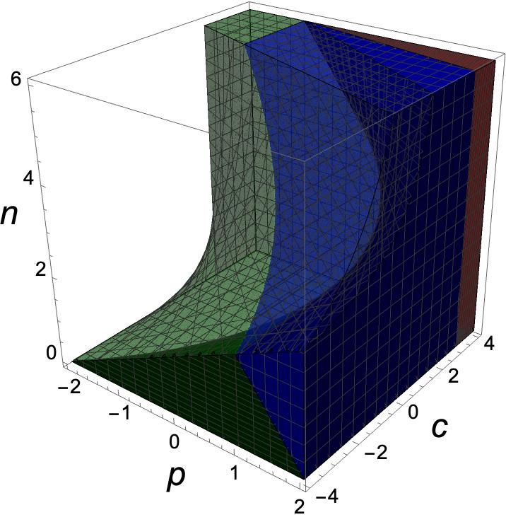
(a)  3d parameter space $(c,p,n)$

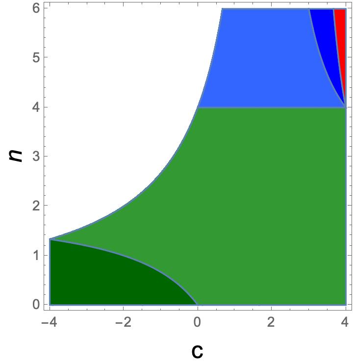
(b)  Plane $p=0$

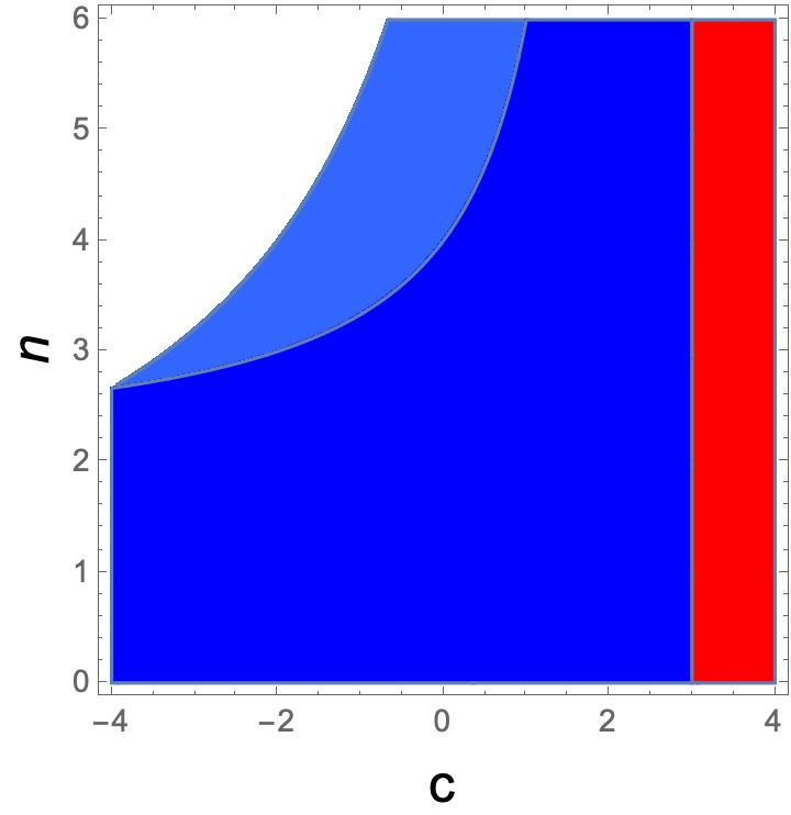
(c)  Plane $p=2$

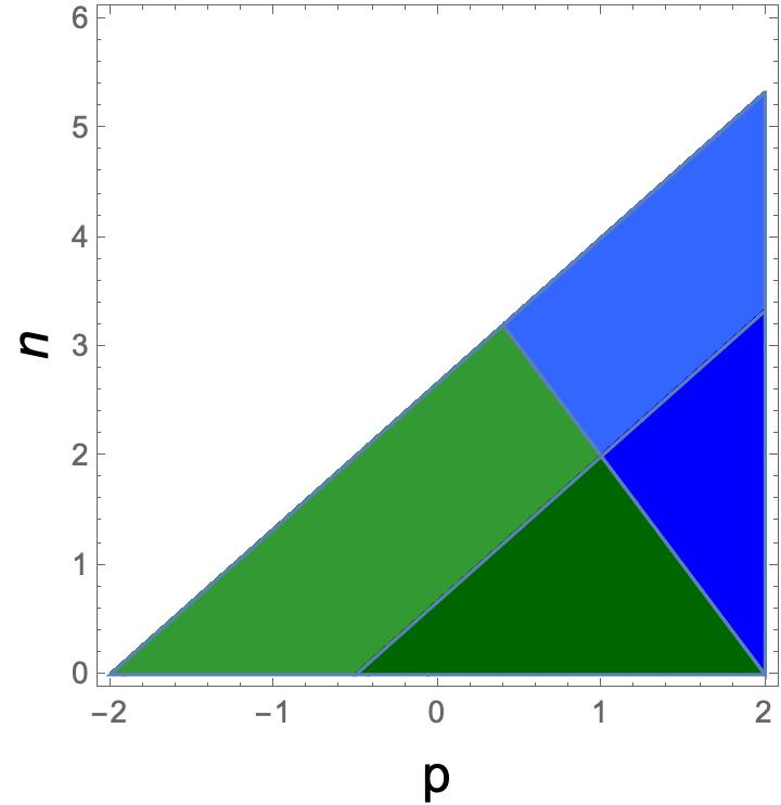
(d)  Plane $c=-1$

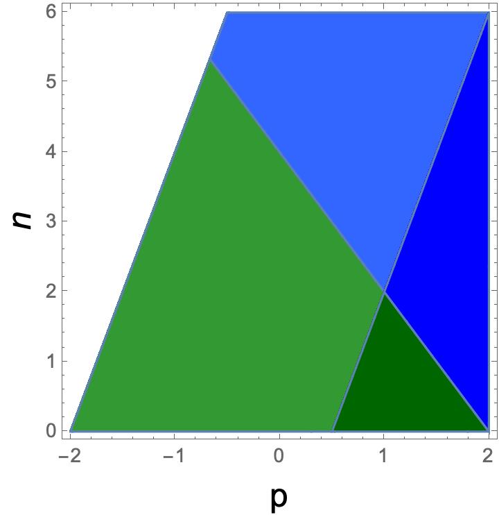
(e)  Plane $c=1$

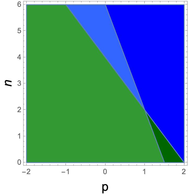
(f)  Plane $c=3$

Figure 1: The parameter space of WI in the weak dissipative regime ($Q<1$) and for the monomial class of inflaton potentials. The shaded areas indicate WI has a graceful exit, while empty (white) space indicates where there is no graceful exit. The shaded areas are classified based on the behavior of $Q$, $T/H$ and $T$ during inflation when all three increase (light green), $Q$ decreases and both $T/H$ and $T$ increase (dark green), $T$ decreases and both $Q$ and $T/H$ increases (light blue), $T/H$ increases and both $Q$ and $T$ decreases (dark blue), and all three decrease (dark red). Figure based on Ref. Das:2020lut .

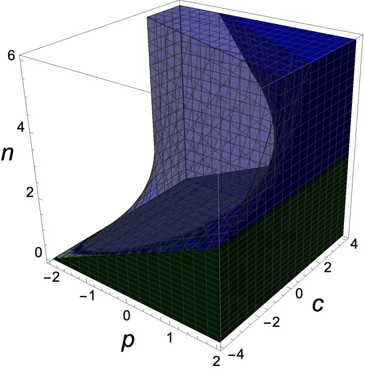
(a)  3d parameter space $(c,p,n)$

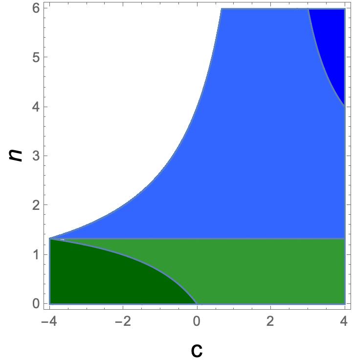
(b)  Plane $p=0$

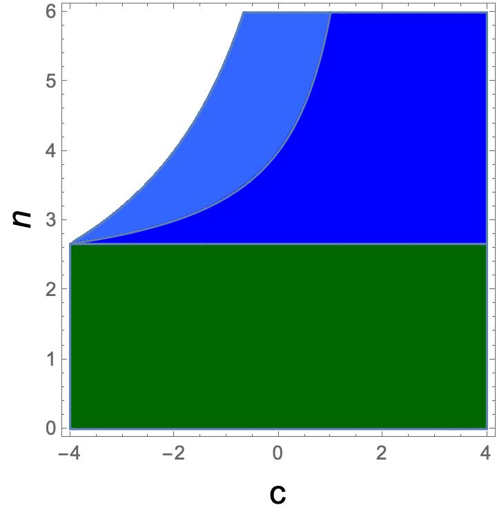
(c)  Plane $p=2$

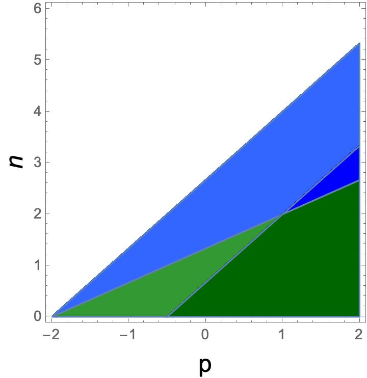
(d)  Plane $c=-1$

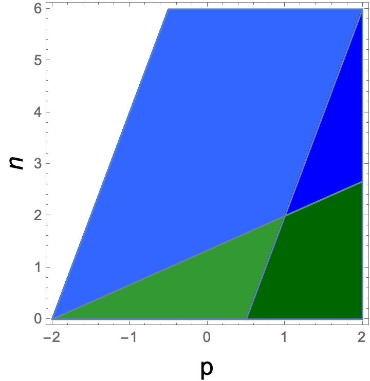
(e)  Plane $c=1$

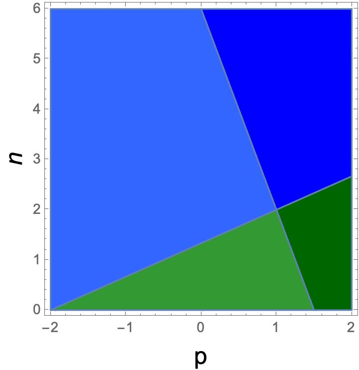
(f)  Plane $c=3$

Figure 2: The parameter space of WI in the strong dissipative regime ($Q>1$) and for the monomial class of inflaton potentials. The shaded areas is classified based on the behavior of $Q$, $T/H$ and $T$ during inflation when all three increase (light green), $Q$ decreases and both $T/H$and $T$ increase (dark green), $T$ decreases and both $Q$ and $T/H$ increase (light blue), and $T/H$ increases and both $Q$ and $T$ decrease (dark blue). Figure based on Ref. Das:2020lut .

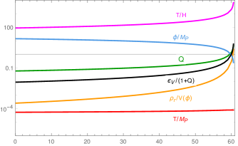
Figure 3: Evolution of the different quantities in the WI scenario for the case of $V(\phi)=\frac{1}{2}m^{2}\phi^{2}$, $\Upsilon=C_{T}T$, with $m=10^{-7}M_{\rm Pl}$ and $C_{T}=0.002$.

Given that, in Fig. 1 we show the space of parameters leading to different scenarios in WI when considering monomial potentials,

$$V(\phi)=\frac{V_{0}}{n}\left(\frac{\phi}{M_{\rm Pl}}\right)^{n},$$ (21)

and for different parametric forms for the dissipation coefficient in the weak dissipative regime. Using Eqs. (17) and (18) and the inequality (15), we find for which values in the space of parameters $(n,c,p)$, WI has graceful exit. One should note that the conditions for WI to have graceful exit is independent of being in the weak or in the strong dissipation regime as it is clear from Eq. (18). Moreover, we also used Eqs. (19) and (20) to see how $T/H$ and $T$ evolve in the region that WI has graceful exit.

In Fig. 2, we also illustrate the space of parameters for WI in the strong dissipation regime to allow to see how the region for evolution for $T/H$ and $T$ change. As we have discussed previously, $Q$ is a dynamical parameter, hence WI may start in the weak dissipative regime and be able to end in the strong dissipative regime, or vice versa. Therefore, $T/H$ and $T$ should not necessarily monotonically increase or decrease during inflation.

Comparing Figs. 1 and 2, one may easily observe that there are possibilities for which $T/H$ and $T$ first increase and then decrease, or vice versa depending on being in the weak or strong dissipation regime and $Q$ increases/decreases.

In Fig. 3, for illustration purposes, the dynamical parameters of WI for a quadratic potential and linear temperature dependent dissipation coefficient are plotted versus the number of e-folding. One can obviously see that the dissipation ratio $Q$, the temperature $T$ and the ratio $T/H$ all increases during the inflationary phase, as it was expected from Fig. 1. Moreover, the radiation to potential energy density increases and become order unity shortly after the end of the inflation. That is because the condition $\epsilon_{V}\simeq 1+Q$ is a weaker condition than $\epsilon_{H}=1$ to specify the end of the inflationary phase in WI scenario. In fact, the first condition points out that inflation ends when $\rho_{r}\simeq V/2$ while in reality one expects that inflation ends when the radiation energy density equals or suppresses the potential energy density as one can see in Fig. 3. In this sense, $\epsilon_{V}\simeq 1+Q$ predicts the end of inflation slightly earlier. In general, the weaker condition only underestimates the end of inflation by less than one e-folding. Thus, the condition $\epsilon_{V}=1+Q$ is still good enough as a way of estimating the instant where WI ends for all practical purposes. Furthermore, the inflaton field starts from super-Planckian values and ends sub-Planckian, with an overall super-Planckian field excursion, which is a typical feature of large field inflationary potentials and, in this case, for WI in the weak dissipative regime, as considered in the example shown in Fig. 3. Sub-Planckian field excursions in WI is possible in the strong dissipative regime of WI, as we will discuss later.

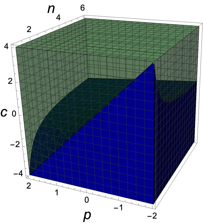
(a)  3d parameter space $(c,p,n)$ in weak dissipative regime

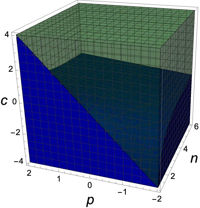
(b)  3d parameter space $(c,p,n)$ in strong dissipative regime

Figure 4: The parameter space in WI for the hiltop-like class of inflaton potentials. The shaded areas indicate WI has a graceful exit, while empty (white) space indicates where there is no graceful exit. The shaded areas is classified based on the behavior of $Q$, $T/H$ and $T$ during inflation when all three increase (dark green), and $Q$ decrease and both $T/H$ and $T$ increase (dark blue). Figure based on Ref. Das:2020lut .

As an additional example, in Fig. 4, we plotted the space of parameters for another class of potential, hiltop-like potentials, given by

$$V(\phi)=V_{0}[1-(\phi/\phi_{0})^{2n}]^{2},$$ (22)

with $n\geq 1$ and with the inflation taking place around the top (plateau) of the potential, $|\phi|\ll\phi_{0}$. We also consider that $\phi_{0}$ is sufficiently large such that inflation ends before the inflection point of the potential. Thus, we are considering that inflation takes place exactly in the concave part of the potential. Notice that here all the parameter space allows for graceful exit, and $T$ and $T/H$ always increase for all space of parameters. Finally, it deserves to be noticed that exponential potentials like

$$V(\phi)=V_{0}\exp({-\alpha{\phi}/{M_{\rm Pl}}}),$$ (23)

can lead to a power law inflation only for $\alpha<\sqrt{2}$ in CI scenario, while it does not have a graceful exit for $\alpha\geq\sqrt{2}$ Copeland:1997et . However, looking at Eq.(11), one can easily observe that the exponential potential not only can result in an accelerated expansion even for $\alpha>\sqrt{2}$, but also it has a graceful exit as long as the dissipation ratio is decreasing during inflation, i.e., when $c>2$, regardless of the value of $p$ for $\alpha\phi/M_{\rm Pl}>1$. This case and other forms of primordial inflaton potentials have been studied in details in Ref. Das:2020lut .

III Deriving dissipation coefficients in WI

The dynamics in WI is intrinsically a result of particle production processes able to happen during inflation. The generic idea is that as the inflaton evolves in time, moving around its potential, it might excite any other fields that are coupled to it. This in turn can produce relativistic particles and maintain a quasi-stationary radiation bath throughout the inflationary regime. At the end of the accelerated inflationary regime, the universe can then smoothly transit to the radiation dominated regime.

Crucial to the idea of WI is then the role played by the dissipation coefficient $\Upsilon$, e.g., in the inflaton effective evolution equation, Eq. (5). As in any inflation model, we expect the inflaton to be necessarily coupled to other fields, which similar to the case of CI as required for reheating, the energy density in the inflaton will eventually be transferred to radiation. The emergence of dissipative processes in this case is reminiscent of the so-called Caldeira and Leggett type of models Caldeira:1982iu . There is a relevant degree of freedom, in which we are interested in the dynamics and that here is the background inflaton field. The system (the inflaton background) is in turn coupled to other degrees of freedom, i.e., any other fields coupled to the inflaton, which are regarded as environmental degrees of freedom. Below, we sketch the general idea for completeness, but which can also be found in details in many other previous papers, in particular in the Refs. Gleiser:1993ea ; Berera:1998gx ; Berera:2001gs ; Berera:2004kc ; Berera:2008ar . We can describe the inflaton field and environment fields through a generic Lagrangian density of the form,

$${\cal L}[\Phi,X,Y]={\cal L}[\Phi]+{\cal L}[X]+{\cal L}[Y]+{\cal L}_{\rm int}[\Phi,X]+{\cal L}_{\rm int}[X,Y],$$ (24)

where here $\Phi$ is the inflaton field, or more specifically its zero mode, represented by the homogeneous background value, while $X$ is describing any field or degrees of freedom coupled directly to the inflaton field (like fermion fields or other bosons that can be scalars or vector fields), while $Y$ can be any other fields not necessarily coupled to the inflaton, like additional bosons and/or fermions, but that can be coupled to $X$. The different interactions are described by the terms in Eq. (24), ${\cal L}_{\rm int}[\Phi,X]$, for the interactions of the inflaton with the $X$ fields, and ${\cal L}_{\rm int}[X,Y]$, for the interactions between $X$ and $Y$, but not directly with the inflaton field.

The evolution of the inflaton field is then determined from Eq. (24) by integrating over the environment fields $X$ and $Y$. This can be done for example in the context of the in-in Schwinger closed-time path functional formalism (for a textbook account, see, for example, Ref. Bellac:2011kqa ) or, equivalently, through the influence functional formalism Calzetta:2008iqa . The formal expression for the evolution for a background field value $\Phi(x)$ turns out to be in the form of a stochastic equation of motion of the form Gleiser:1993ea ; Berera:1998gx ; Berera:2008ar

$$\partial^{2}\Phi+V_{\rm eff}^{\prime}(\Phi)+\int d^{4}x^{\prime}{\cal D}^{(X)}(x,x^{\prime})\dot{\Phi}_{c}(x^{\prime})=\xi(x),$$ (25)

where $V_{\rm eff}^{\prime}(\Phi)=dV_{\rm eff}(\Phi)/d\Phi$, with $V_{\rm eff}(\Phi)$ being the effective potential for $\Phi$. The term with ${\cal D}^{(X)}(x,x^{\prime})$, defined as

$$\Sigma^{(X)}_{\rho}(x,x^{\prime}){\rm sgn}(t-t^{\prime})=-\frac{\partial}{\partial t^{\prime}}{\cal D}^{(X)}(x,x^{\prime}),$$ (26)

describes the dissipative effects due to the interaction of the inflaton with the environment fields, while $\xi(x)$ represents stochastic noise fluctuations, which affect the dynamics of $\Phi_{c}$ and describe Gaussian processes with the general properties of having zero mean, $\langle\xi(x)\rangle=0$, and two-point correlation function given by

$$\langle\xi(x)\xi(x^{\prime})\rangle=\Sigma_{F}^{(X)}[\Phi_{c}](x,x^{\prime}).$$ (27)

In Eqs. (26) and (27), $\Sigma^{(X)}_{\rho}$ and $\Sigma_{F}^{(X)}$ are the self-energy terms in the Schwinger-Keldshy real time formalism of quantum field theory Calzetta:2008iqa . Furthermore, both noise and dissipation terms are related to each other through a generalized fluctuation dissipation relation Berera:2008ar , as expected for a Langevin-like evolution describing a stochastic process under both dissipation and noise terms.

If the field $\Phi$ is slowly varying on the response timescale $1/\Gamma$, with the $\Gamma$ derived from the self-energies terms coming from the $X$ and $Y$, then $\dot{\Phi}/\Phi\ll\Gamma$. Under these conditions, which are typically referred to as the adiabatic approximation, then a simple Taylor expansion of the non-local terms in Eq. (25) can be performed. Furthermore, if $\Gamma>H$, the produced radiation through the dissipative processes can be thermalized sufficiently fast. Under the further adiabatic condition that $\Gamma\gg\dot{T}/T$, then it is expected that the produced radiation can be maintained in a close to thermal equilibrium state at a temperature $T$. These conditions provide a clear separation of timescales in the system, which allows to approximate Eq. (25) in the form of a local, Markovian equation of motion Berera:2007qm , with a local dissipation coefficient $\Upsilon$ defined by

$$\Upsilon=\int d^{4}x^{\prime}\,\Sigma_{R}[\Phi](x,x^{\prime})\,(t^{\prime}-t),$$ (28)

where $\Sigma_{R}^{(X)}(x,x^{\prime})=\Sigma^{(X)}_{\rho}(x,x^{\prime})\theta(t-t^{\prime})$ is a retarded self-energy term. Overall, the Eq. (25), when working in a Friedmann-Lemaître-Robertson-Walker (FLRW) background metric, then becomes of the form

$$\left[\frac{\partial^{2}}{\partial t^{2}}+(3H+\Upsilon)\frac{\partial}{\partial t}-\frac{1}{a^{2}}\nabla^{2}\right]\Phi+\frac{\partial V_{\rm eff}(\Phi)}{\partial\Phi}=\xi_{T},$$ (29)

where $\xi_{T}$ describes thermal (Gaussian and white) noise fluctuations in the local approximation as defined above and it is connected to the dissipation coefficient through a Markovian fluctuation-dissipation relation,

$$\langle\xi_{T}({\bf x},t)\xi_{T}({\bf x}^{\prime},t^{\prime})\rangle=2\Upsilon Ta^{-3}\delta({\bf x}-{\bf x}^{\prime})\delta(t-t^{\prime}),$$ (30)

where the average here is to be interpreted as been taken over the statistical ensemble. Stochastic terms can also be ascribed for quantum contributions and will be important when deriving the perturbations equations. This will be discussed in the next section, Sec. IV.

The effective evolution equation for the inflaton, Eq. (5), then follows from the localized form for the effective equation of motion, Eq. (29) by separating the background field into its homogeneous term $\phi(t)$. On the other hand, the non-homogeneous fluctuations over $\phi(t)$, denoted as $\delta\phi({\bf x},t)$, will describe the fluctuations of the inflaton and to be considered in the density perturbation equations (see, next section). The latter are explicitly dependent on the stochastic noise term. From the above definitions, once a particular interaction Lagrangian density is given, the corresponding dissipation term $\Upsilon$ can be computed explicitly. Various examples of interactions and the resulting dissipation terms have been derived and given, e.g., in Ref. Bastero-Gil:2010dgy .

Below, we will summarize some of the most important microscopic particle physics constructions considered for WI. As already explained before, the particle physics implementation for WI seeks models for which a significant dissipation can be generated during inflation and at the same time the radiative and thermal corrections for the inflaton potential are kept under control, such that the flatness of the inflaton potential is not spoiled. The first particle physics models constructions in WI achieved this using quantum field theory models in supersymmetry (SUSY). This is the case of the first two models described below.

III.1 The distributed mass model

In the distributed mass model (DMM) Berera:1998px , there are a set of scalar $\chi_{j}$ and fermionic $\psi_{j}$ fields coupled to the inflaton through a series of couplings of the form $g^{2}(\phi-M_{j})^{2}\chi_{j}^{2}$ and $h(\phi-M_{j})\bar{\psi}_{j}\psi_{j}$, respectively. The idea is that as the inflaton is evolving, eventually the inflaton satisfies $\phi\sim M_{j}$. At this point, the masses of the fields coupled to it can become very light. In special, as these masses become smaller than the temperature, those fields will get thermally excited and the inflaton will be able to decay into those fields. A sequence of mass distributions $M_{j}$ can then be constructed in such a way that as the background inflaton field evolves, it is able to dissipate energy into these fields throughout the inflationary regime. This process can then be described by a dissipative term in the inflaton evolution equation Berera:1998gx . The idea is reminiscent of string theory model constructions Berera:1999wt . In this case, the inflaton is interpreted as an excited string zero mode. This string mode can then be interacting with massive string levels. As the string levels can be highly degenerate, a distribution of mass states can emerge as a type of fine structure splitting of those levels. The DMM realization for WI was also revised more recently in Ref. Bastero-Gil:2018yen . Both radiative and thermal corrections coming from the large set of bosonic and fermionic fields coupled to the inflaton can be well controlled by constructing the DMM in the context of SUSY. Despite the inflaton background field and thermal effects both break supersymmetry, there are still large cancellations between fermions and bosons contributions Hall:2004zr . The DMM can be implemented by a superpotential in the context of SUSY, given by

$$W=\sum_{j}\left[\frac{g}{2}(\Phi-M_{j})X_{j}^{2}+\frac{h}{2}X_{j}Y_{j}^{2}\right],$$ (31)

where $\Phi$, $X_{j}$ and $Y_{j}$ chiral superfields, with (complex) scalar and fermion components $\varphi$ and $\psi_{\varphi}$ for $\Phi$, $\chi_{j}$ and $\psi_{\chi_{j}}$ for $X_{j}$, and $\sigma_{j}$ and $\psi_{\sigma_{j}}$ for $Y_{j}$. The inflaton is associated with the real component of $\varphi$. The $g$ and $h$ are coupling constants and the sum is taken over an arbitrary distribution of supermultiplets $X_{j}$ and $Y_{j}$. From Eq. (31), we can derive the scalar $\mathcal{L}_{S}$ and fermionic $\mathcal{L}_{F}$ Lagrangian density interaction terms, which are defined, respectively, as Hall:2004zr

$$-\mathcal{L}_{S}=|\partial_{\Phi}W|^{2}+\sum_{j}|\partial_{X_{j}}W|^{2}+\sum_{j}|\partial_{Y_{j}}W|^{2},$$ (32)

and

$$-\mathcal{L}_{F}=\frac{1}{2}\sum_{n,m}\frac{\partial^{2}W}{\partial\xi_{n}\partial\xi_{m}}\bar{\psi}_{n}P_{L}\psi_{m}+\frac{1}{2}\sum_{n,m}\frac{\partial^{2}W^{\dagger}}{\partial\xi^{\dagger}_{n}\partial\xi^{\dagger}_{m}}\bar{\psi}_{n}P_{R}\psi_{m},$$ (33)

where $\xi_{n}$ is a superfield: $\Phi,X_{j},Y_{j}$ and $P_{L}=1-P_{R}=(1+\gamma_{5})/2$ are the chiral projection operators acting on Majorana 4-spinors. The expressions Eqs. (32) and (33), then lead to the explicit Lagrangian density relevant contributions that are given by Bastero-Gil:2018yen

$$-\mathcal{L}_{S} = g^{2}\sum_{j}\left(\phi-M_{j}\right)^{2}|\chi_{j}|^{2}+\frac{gh}{2}\sum_{j}\left(\phi-M_{j}\right)\left[\chi_{j}(\sigma_{j}^{\dagger})^{2}+\chi_{j}^{\dagger}\sigma_{j}^{2}\right]$$ (34)

$$+h^{2}\sum_{j}|\chi_{j}|^{2}|\sigma_{j}|^{2}+\frac{g^{2}}{4}\sum_{j}|\chi_{j}|^{4}+\frac{h^{2}}{4}\sum_{j}|\sigma_{j}|^{4},$$

and

$$-\mathcal{L}_{F} = \frac{g}{2}\sum_{j}\left(\phi-M_{j}\right)\bar{\psi}_{\chi_{j}}P_{L}\psi_{\chi_{j}}+\frac{g}{2}\sum_{j}\left(\phi-M_{j}\right)\bar{\psi}_{\chi_{j}}P_{R}\psi_{\chi_{j}}$$ (35)

$$+\frac{h}{2}\sum_{j}\chi_{j}\bar{\psi}_{\sigma_{j}}P_{L}\psi_{\sigma_{j}}+\frac{h}{2}\sum_{j}\chi^{\dagger}_{j}\bar{\psi}_{\sigma_{j}}P_{R}\psi_{\sigma_{j}}+h\sum_{j}\sigma_{j}\bar{\psi}_{\sigma_{j}}P_{L}\psi_{\chi_{j}}+h\sum_{j}\sigma^{\dagger}_{j}\bar{\psi}_{\sigma_{j}}P_{R}\psi_{\chi_{j}}.$$

From the interactions terms in Eqs. (34) and (35), we can determine the dissipation coefficient $\Upsilon$, which will receive contributions both from the scalar bosons Berera:1998gx ; Berera:1998px (see also Ref. Bastero-Gil:2018yen for details)

$$\Upsilon^{S}(\phi,T)=\sum_{j=1}^{N_{th}}\frac{32g^{4}}{\pi h^{2}\left(16\frac{m_{\chi_{j}}^{2}}{\tilde{m}_{\chi_{j}}^{2}}+\frac{\tilde{m}_{\chi j}^{2}}{T^{2}}\right)}\ln\left(\frac{2T}{\tilde{m}_{\chi_{j}}}\right)\frac{\left(\phi-M_{j}\right)^{2}}{\tilde{m}_{\chi_{j}}},$$ (36)

and from the fermions Bastero-Gil:2016qru ,

$$\Upsilon^{F}(T)=\sum_{j=1}^{N_{th}}C_{T}^{F}T\,,\quad C_{T}^{F}\simeq\frac{3g^{2}}{h^{2}[1-0.34\ln(h)]}\,,$$ (37)

where in the above equations, the sum run over the number $N_{th}$ of thermally excited field modes and the masses $m_{\chi_{j}}$ and $\tilde{m}_{\chi_{j}}$ are defined, respectively, as $m_{\chi_{j}}=g\left(\phi-M_{j}\right)$ and $\tilde{m}_{\chi_{j}}^{2}=m_{\chi_{j}}^{2}+g^{2}T^{2}/12+h^{2}T^{2}/8$. One notes that the dissipation coefficient in the DMM depends on the mass distribution $M_{j}$. Assuming Bastero-Gil:2018yen $M_{j}=\phi+j\Delta M(\phi,T,m,g)$, where $\Delta M$ denotes the mass gap in the tower of states, different functional forms for the dissipation coefficient in the DMM can be generated through different choices of $\Delta M(\phi,T,m,g)$. This motivates the parametric choice Eq. (16) adopted in many works in WI.

III.2 The two-stage mechanism model

Without a way of controlling the thermal corrections of the radiation fields that are directly coupled to the inflaton, it is expected that the finite temperature of the radiation bath will induce large thermal corrections to the inflaton mass, leading to $m_{\phi}\sim T>H$. If this occurs, successful realizations of WI in the simplest models are jeopardized. In this case, the additional friction caused by the dissipation effects through $\Upsilon$ cannot overcome the increase in the inflaton’s mass. In the DMM discussed above, even though there are couplings of the inflaton directly to the radiation fields, it is able to evade this problem by a judicious choice of the mass distribution function. But in other model realizations this is not a simple task to achieve, as discussed originally in Refs. Berera:1998gx ; Yokoyama:1998ju . However, we also recall that fields that are directly coupled to the inflaton will tend to acquire large masses during inflation due to the large background field value $\phi$. This then suggests that WI can be better implemented in scenarios where the inflaton does not couple directly to the radiation fields, but instead to heavy intermediate fields, which can be either bosons or fermions, with masses such that $m_{\chi},\,m_{\psi}>T$. This naturally leads to thermal corrections to the inflaton potential that are Boltzmann suppressed. Furthermore, once again, we can use SUSY to control potentially large radiative corrections to the inflaton. In turn, the heavy fields can be made coupled to the radiation fields, which remain decoupled from the inflaton sector. Once again, as the inflaton dynamics change the masses of the heavy fields, these can decay into the light radiation fields. These processes provide a way through which the inflaton can dissipate its energy into radiation. A significant dissipation can be generated depending on the field multiplicities. This is the two-stage decay mechanism model for WI.

The two-stage mechanism for WI can be implemented through a supersymmetric model with chiral superfields $\Phi$, $X$ and $Y_{i}$, $i=1,\ldots,N_{Y}$, and described by the superpotential

$$W={g\over 2}\Phi X^{2}+{h_{i}\over 2}XY_{i}^{2}+f(\Phi)~{},$$ (38)

where a sum over the index $i$ is implicit. The scalar component of the superfield $\Phi$ describes the inflaton field, with an expectation value $\phi/\sqrt{2}$, which we assume to be real, and the generic holomorphic function $f(\Phi)$ describes the self-interactions in the inflaton sector. The superpotential Eq. (38) leads to the Lagrangian density describing the interactions between the inflaton field $\phi$ with the other scalars and fermions as given by Bastero-Gil:2012akf

$$\mathcal{L}_{scalar} = V(\phi)+{1\over 2}g^{2}\phi^{2}|\chi|^{2}+{g\over 2}\sqrt{V(\phi)}\left(\chi^{2}+\chi^{\dagger 2}\right)+{g^{2}\over 4}|\chi|^{4}+$$ (39)

$$+ {h_{i}\over 2}{g\phi\over\sqrt{2}}\left(\chi\sigma_{i}^{\dagger 2}+\chi^{\dagger}\sigma_{i}^{2}\right)+{h_{i}h_{j}\over 4}\sigma_{i}^{2}\sigma_{j}^{\dagger 2}+h_{i}^{2}|\chi|^{2}|\sigma_{i}|^{2}~{},$$

and

$$\mathcal{L}_{fermion} = {g\phi\over\sqrt{2}}\bar{\psi}_{\chi}P_{L}\psi_{\chi}+h_{i}\chi\bar{\psi}_{\sigma_{i}}P_{L}\psi_{\sigma_{i}}+{h_{i}\over 2}\sigma_{i}\bar{\psi}_{\sigma_{i}}P_{L}\psi_{\chi}+\mathrm{h.c.}~{},$$ (40)

where the scalar components of the superfields $X$ and $Y_{i}$ were denoted by $\chi$ and $\sigma_{i}$, respectively, the fermionic components by $\psi_{\chi}$ and $\psi_{\sigma_{i}}$, respectively , $V(\phi)=|f^{\prime}(\phi)|^{2}$ is the potential driving inflation and $P_{L}=(1-\gamma_{5})/2$ is the left-handed chiral projector.

The leading dissipation coefficient obtained for this model and using the quantum field theory expression Eq. (28), can be explicitly derived and it is given by Bastero-Gil:2010dgy :

$$\Upsilon={4\over T}\left({g^{2}\over 2}\right)^{2}\varphi^{2}\int{d^{4}p\over(2\pi)^{4}}\rho_{\chi}^{2}n_{B}(1+n_{B})~{},$$ (41)

where $n_{B}(p_{0})=[e^{p_{0}/T}-1]^{-1}$ is the Bose-Einstein distribution and $\rho_{\chi}$ is the spectral function for the $\chi$ field,

$$\rho_{\chi}(p_{0},p)={4\omega_{p}\Gamma_{\chi}\over(p_{0}^{2}-\omega_{p}^{2})^{2}+4\omega_{p}^{2}\Gamma_{\chi}^{2}}~{},$$ (42)

with $\Gamma_{\chi}$ denoting the decay width for the heavy fields $\chi$, which includes contributions from both the bosonic and fermionic final states in the $Y_{i}$ multiplets, $\omega_{p}=\sqrt{\tilde{m}_{\chi}^{2}+p^{2}}$ for modes of 3-momentum $|\mathbf{p}|=p$ and energy $p_{0}$, while the thermal mass for the $\chi$ fields is $\tilde{m}_{\chi}^{2}=m_{\chi}^{2}+h^{2}N_{Y}T^{2}/8$ (where here we are assuming all couplings $h_{i}=h$) and $m_{\chi}=g\phi/\sqrt{2}$. For larger values of the mass and effective coupling, the main contribution to the dissipation coefficient comes from virtual $\chi$ modes with low momentum and energy, $p,p_{0}\ll m_{\chi}$, such that one can use the approximation $(p_{0}^{2}-\omega_{p}^{2})^{2}\simeq\tilde{m}_{\chi}^{4}$. In the case where these modes also have a narrow width and thermal mass corrections can be neglected, $\Gamma_{\chi}\ll\tilde{m}_{\chi}\sim m_{\chi}$, then the spectral function Eq. (42) can be simply expressed as Berera:2008ar ; Bastero-Gil:2010dgy $\rho_{\chi}\simeq 4\Gamma_{\chi}/m_{\chi}^{3}$. Under these circumstances, the dissipation coefficient $\Upsilon$ describing the dissipation mediated by the decay of virtual scalar modes $\chi\rightarrow{\rm light\,radiation\,fields}$, is given by Bastero-Gil:2012akf

$$\Upsilon=C_{\phi}{T^{3}\over\phi^{2}}~{},\qquad C_{\phi}\simeq{1\over 4}\alpha_{h}N_{X}~{},$$ (43)

for $\alpha_{h}=h^{2}N_{Y}/4\pi\lesssim 1$ and $N_{X,Y}$ are the chiral multiplets.

To obtain sufficient dissipation in these models, it is usually required large values for the numbers of multiplets $N_{X,Y}$. While these can be seen as a possible drawback for this model, there are well motivated scenarios where this can be naturally achieved, like in Ref. Bastero-Gil:2011zxb using brane constructions, or like in Ref. Matsuda:2012kc , where large field multiplicities can be allowed due to a Kaluza-Klein tower in extra-dimensional scenarios.

Instead of relying on SUSY as a way to suppress radiative corrections, we can try to arrange for special interactions of the inflaton with the environment fields such as to be able to control the thermal corrections to the inflaton potential. This can also be used to avoid the large multiplicities that would otherwise be required to produce sufficiently large dissipation, such that WI can be realized. To avoid these complications, we can make use of other simpler models exploring well motivated symmetry properties for the interactions. This is the case for the next three particle physics model constructions for WI to be discussed below.

III.3 The warm little inflaton model

In the warm little inflaton (WLI) model, first introduced in Ref. Bastero-Gil:2016qru , the inflaton is assumed to be a pseudo-Nambu-Goldstone boson (PNGB) of a gauge symmetry that is collectively broken. The idea is reminiscent of the “Little Higgs” models of electroweak symmetry breaking ArkaniHamed:2001nc ; Kaplan:2003aj ; ArkaniHamed:2003mz , where the Higgs boson is also considered to be a PNGB coming from a collectively broken global symmetry. A feature displayed by the type of construction in these type of models is that the PNGB has a mass that is naturally protected against large radiative corrections (for a review, see, e.g., Ref. Schmaltz:2005ky ).

The construction of the WLI model uses a very minimum set of ingredients. There are two complex scalar fields, $\phi_{1}$ and $\phi_{2}$, which share the same $U(1)$ symmetry. The scalar potential for them allow both fields to have a nonzero vacuum expectation value, $\langle\phi_{1}\rangle=\equiv M_{1}/\sqrt{2}$ and $\langle\phi_{2}\rangle\equiv M_{2}/\sqrt{2}$, where $M_{1}$ can be taken to be equal to $M_{2}$ without loss of generality, $M_{1}=M_{2}\equiv M$. With both fields sharing the same Abelian charge, after the Higgs mechanism, only one the phases of the complex scalar fields (the Nambu-Goldstone boson), or a linear combination of them, is absorbed as the longitudinal component of the $U(1)$ gauge boson, providing mass to it. The other phase (or linear independent combination of the phases) remains, however, as a physical degree of freedom, becoming, e.g., a singlet. The two complex scalar fields, in the broken phase, can then be expressed in the form

$$\phi_{1}={M\over\sqrt{2}}e^{i\phi/M}~{},\qquad\phi_{2}={M\over\sqrt{2}}e^{-i\phi/M}.$$ (44)

The radial modes in Eq. (44) decouple when $M\gtrsim T$ and the singlet $\phi$, the PNBG, is taken to be the inflaton. One notes that as such, we can assume for $\phi$ an arbitrary scalar potential that can be sufficiently flat to sustain inflation. Dissipation in the model comes from the coupling of $\phi_{1}$ and $\phi_{2}$ to other fields. For example, they can be coupled to left-handed fermions $\psi_{1}$ and $\psi_{2}$ with the same $U(1)$ charge of the scalar fields. The right-handed components of these fermion fields, $\psi_{1R}$ and $\psi_{2R}$, can be taken to be gauge singlets, in a construction similar as in the Glashow-Weinberg-Salam of the standard model of particle physics. A decay width for these fermions, which will contribute to the dissipation coefficient, can be generated by coupling them to additional Yukawa interactions, involving a scalar singlet $\sigma$ and chiral fermions $\psi_{\sigma R}$, carrying the same charge of $\psi_{1}$ and $\psi_{2}$, and $\psi_{\sigma L}$, with zero charge. For all these fields, we impose an interchange symmetry for the complex scalars $\phi_{1}$ and $\phi_{2}$, $\phi_{1}\leftrightarrow i\phi_{2}$, and also for the fermions $\psi_{1}$ and $\psi_{2}$, $\psi_{1L,R}\leftrightarrow\psi_{2L,R}$. The overall interaction Lagrangian density is Bastero-Gil:2016qru

$${\cal L}_{\rm int}=\mathcal{L}_{\phi\psi}+\mathcal{L}_{\psi\sigma},$$ (45)

with

$$\mathcal{L}_{\phi\psi} = -{g\over\sqrt{2}}(\phi_{1}+\phi_{2})\bar{\psi}_{1L}\psi_{1R}+i{g\over\sqrt{2}}(\phi_{1}-\phi_{2})\bar{\psi}_{2L}\psi_{2R},$$ (46)

and

$$\mathcal{L}_{\psi\sigma}=-h\sigma\sum_{i=1,2}\left(\bar{\psi}_{iL}\psi_{\sigma R}+\bar{\psi}_{\sigma L}\psi_{iR}\right),$$ (47)

which respects the symmetries imposed on the model. Due to the symmetries, and using Eq. (44), the masses for the fermions $\psi_{1}$ and $\psi_{2}$, $m_{1}$ and $m_{2}$, respectively, are then given by

$$m_{1}=gM\cos(\phi/M),\;\;\;m_{2}=gM\sin(\phi/M),$$ (48)

and, hence, they remain always bounded, $m_{1,2}\leq gM$, and they can be arranged to remain light during inflation if $gM\lesssim T\lesssim M$. The advantage of the interactions in Eq. (46) is that they lead to no quadratic corrections for $\phi$ in the inflaton potential, thus, the inflaton mass does not receive neither radiative nor thermal corrections. The inflaton potential is only affected by subleading Coleman-Weinberg corrections, as it was demonstrated in Ref. Bastero-Gil:2016qru .

With the above interactions, the dissipation coefficient for the WLI model becomes Bastero-Gil:2016qru

$$\Upsilon=C_{T}T~{},\qquad C_{T}\simeq\alpha(h)g^{2}/h^{2}~{},$$ (49)

where $\alpha(h)\simeq 3/[1-0.34\ln(h)]$.

The model has also been shown to produce a well-motivated dark matter candidate Rosa:2018iff . This can be possible because soon after inflation, the fermions coupled to the inflaton field are no longer light. The dissipation coefficient Eq. (49) becomes Boltzmann suppressed. For an inflaton potential augmented by quadratic term with a mass term $m_{\phi}$, then, when $H<m_{\phi}$, the inflaton field is underdamped and it will oscillate around the minimum of its potential. The equation of state oscillates around $w_{\phi}=0$, and the energy density scales as $\rho_{\phi}\propto 1/a^{3}$. This is the same behavior as ordinary matter. Due to the symmetries of the model, the inflaton rarely decays and an abundance of inflaton energy density can remain in the coherent oscillating state. This makes the inflaton in the WLI model to be a possible valid dark matter candidate.

III.4 The warm little inflaton model - scalar version

A variant Bastero-Gil:2019gao of the WLI model discussed above is when the complex scalar fields $\phi_{1}$ and $\phi_{2}$ are now coupled directly to other two complex scalar fields $\chi_{1}$ and $\chi_{2}$, instead of fermions. As in the previous model, it is also imposed the discrete interchange symmetry $\phi_{1}\leftrightarrow i\phi_{2}$, $\chi_{1}\leftrightarrow\chi_{2}$. The complex scalar fields $\chi_{1,2}$ can also have a Yukawa interaction to fermions, self-interact and also interact between each other. Then, the interacting Lagrangian density can now be expressed as Bastero-Gil:2019gao

$${\cal L}_{\rm int}=\mathcal{L}_{\phi\chi}+\mathcal{L}_{\chi\psi},$$ (50)

with

$$\mathcal{L}_{\phi\chi}=-{1\over 2}g^{2}|\phi_{1}+\phi_{2}|^{2}|\chi_{1}|^{2}-{1\over 2}g^{2}|\phi_{1}-\phi_{2}|^{2}|\chi_{2}|^{2},$$ (51)

and

$$\mathcal{L}_{\mathrm{\chi\psi}}\!=\!\!\!\!\!\sum_{\begin{subarray}{c}i\neq j=1,2\end{subarray}}\!\!\!\left(h\chi_{i}\bar{\psi}_{L}\psi_{R}\!+\!\mathrm{h.c.}\!-\!{\lambda\over 2}|\chi_{i}|^{4}\!-\!{\lambda^{\prime}}|\chi_{i}|^{2}|\chi_{j}|^{2}\!\right)\!.$$ (52)

One notes that under the parametrization given by Eq. (44), the masses for the scalar fields $\chi_{1}$ and $\chi_{2}$ are still of the same form as in Eq. (48). Hence, they are still bounded and can be light with respect to the temperature just the same way as in the previous model. In the high temperature regime, $m_{1,2}\ll T$, the inflaton potential receives leading order thermal corrections of the form $m_{1}^{2}(\phi)T^{2}/12+m_{1}^{2}(\phi)T^{2}/12=g^{2}M^{2}T^{2}/12$ and, thus, the inflaton mass here also does not receive any thermal corrections, while also not receiving any important radiative contributions.

In this scalar field variant of the WLI model, the dissipation coefficient now becomes Bastero-Gil:2019gao

$$\Upsilon\simeq{4g^{4}\over h^{2}}{M^{2}T^{2}\over\tilde{m}_{\chi}^{3}}\left[1+{1\over\sqrt{2\pi}}\left({\tilde{m}_{\chi}\over T}\right)^{3/2}\right]e^{-\tilde{m}_{\chi}/T},$$ (53)

where we have taken the average of the oscillatory terms for field excursions $\Delta\phi\gg M$ and $\tilde{m}_{\chi}$ is the thermal mass for the $\chi_{1,2}$ fields, which, under the same average over the oscillatory terms, is the same for both scalars and given by $\tilde{m}_{\chi}^{2}\simeq g^{2}M^{2}/2+\alpha^{2}T^{2}$, where $\alpha^{2}\simeq\left[h^{2}+2\lambda+\lambda^{\prime}\right]/12$ when taking the interactions in Eq. (52). It is noticed that when considering the leading thermal contribution in $\tilde{m}_{\chi}$, i.e., $\tilde{m}_{\chi}\sim\alpha T$, the dissipation coefficient (53) varies with the temperature as $\Upsilon(T)\propto T^{-1}$, realizing the case with $c=-1,p=0$ in Eq. (16). On the other hand, as the temperature of the thermal bath drops and the vacuum term $gM/\sqrt{2}$ in $\tilde{m}_{\chi}$ starts no longer to be negligible, it effectively would correspond to values of $c>-1$, with a limiting case of $c=2$ when $gM/\sqrt{2}\gg\alpha T$ and with an exponentially suppressed dissipation. As shown in Ref. Bastero-Gil:2019gao , this more complex behavior for the dissipation coefficient with the temperature of the environmental radiation bath makes it possible to produce a large dissipative regimes for WI, in which $Q\gg 1$ can be achieved in this model, with perturbations still consistent with the CMB measurements. On the other hand, the dissipation coefficient in the previous model, Eq. (49), in general can only produce perturbations consistent with the CMB observations in the weak dissipative regime of WI, i.e., $Q\ll 1$ (see, e.g., Ref. Benetti:2016jhf ). As this version of the WLI allows WI to be realized in the strong dissipative regime, the cosmological phenomenology that it allows is much richer and has quite appealing features, as we will see in the next section, Sec. V.

III.5 The axion-like warm inflaton model

A Goldstone boson $\phi$ enjoys a shift symmetry, with only derivatives of $\phi$ appearing in the action. This symmetry can still be softly broken such as to give $\phi$ an ultraviolet (UV) potential and the Goldstone boson becoming a PNGB, like in axion-like models. But even with the soft breaking of the shift symmetry, radiative and thermal corrections to the axion potential are naturally suppressed by the symmetry properties. This is how axions, for instance, can have very small masses, but that are still protected from large quantum corrections (for a general review on axions and their properties, see, e.g., Ref. Marsh:2015xka ). Thus, it is natural to try to construct WI by taking the inflaton as an axion-like field. One such successful construction was given in Ref. Berghaus:2019whh . The relevant interaction of the inflaton $\phi$ in this case is as in an axion interacting with a Yang-Mills field $A_{\mu}^{a}$ and with Lagrangian density given by

$${\cal L}_{\rm int}=\frac{\alpha_{g}}{8\pi}\frac{\phi}{f}\tilde{F}^{a\,\mu\nu}F^{a}_{\mu\nu},$$ (54)

where $\tilde{F}^{a\,\mu\nu}$ is the dual gauge field strength, $\tilde{F}^{a\,\mu\nu}=\frac{1}{2}\epsilon^{\mu\nu\alpha\beta}F^{a}_{\alpha\beta}$, $F_{\mu\nu}^{a}=\partial_{\mu}A_{\nu}^{a}-\partial_{\nu}A_{\mu}^{a}+gC^{abc}A_{\mu}^{b}A_{\nu}^{c}$, with $g$ the Yang-Mills coupling and $C^{abc}$ is the structure constant of the non-Abelian group. The coupling constant $\alpha_{g}$ is $\alpha_{g}\equiv g^{2}/(4\pi)$ with $f$ denoting a scale analogous to the axion decay constant in axion-like models Marsh:2015xka .

The interaction term Eq. (54) leads to a dissipation coefficient that has been shown to be related to the Chern-Simons diffusion rate Moore:2010jd ; Laine:2016hma and given by

$$\Upsilon=C_{\Upsilon}\frac{T^{3}}{f^{2}},\;\;\;C_{\Upsilon}=\kappa(\alpha_{g},N_{c},N_{f})\alpha_{g}^{5},$$ (55)

where $N_{c}$ is the dimension of the gauge group, $N_{f}$ is the representation of the fermions if any, and $\kappa$ is a dimensional quantity depending on $N_{c}$, $N_{f}$ and $\alpha_{g}$.

Successful WI dynamics have been shown to be possible in this model Berghaus:2019whh ; Goswami:2019ehb ; Laine:2021ego ; DeRocco:2021rzv . These studies have also shown the generality of WI in this type of model. Even by starting with quantum initial conditions for inflation, e.g., like in CI, the dissipative effects naturally drive the production of a radiation bath and that can thermalize during inflation in these axion-type of models. Hence, a WI dynamics naturally emerges given appropriate parameters in the model Laine:2021ego ; DeRocco:2021rzv . Besides of these attractive features, like in the scalar field variant of the WLI model, the dissipation coefficient Eq. (55) has the appeal of leading to WI in the strong dissipative regime $Q\gg 1$, yet, still being fully consistent with the CMB perturbations for many different potentials (for a recent exposition on this and a detailed computation of relevant observable quantities, see, e.g., Ref. Das:2022ubr ). This will be explicitly shown in the next section. Besides, it has a minimum setting of parameters and field ingredients that are necessary to lead to WI. This makes this construction specially attractive from the point of view of model building in WI, as far as its simplicity is concerned.

IV Cosmological Perturbations in WI

As we discussed previously in Sec.II, when $T>H$ thermal fluctuations of the inflaton field will become dominant. As a consequence of this, the source of density fluctuations in the WI scenario is the thermal fluctuations in the radiation field, which are then transferred to the inflaton field as adiabatic curvature perturbations. This is much different than in the CI case, where quantum fluctuations are responsible for generating the seeds for large scale structure formation. We will discuss here how dissipative effects change the dynamics of inhomogeneous fluctuations of the inflaton field. To study the scalar perturbations for WI, we start with the fully perturbed FLRW metric (here we are including only scalar perturbations), which is given by

$$ds^{2}=-(1+2\alpha)dt^{2}-2a\partial_{i}\beta dx^{i}dt+a^{2}\left[\delta_{ij}(1+2\varphi)+2\partial_{i}\partial_{j}\gamma\right]dx^{i}dx^{j},$$ (56)

where $\alpha$, $\beta$, $\gamma$, and $\varphi$ are the spacetime-dependent perturbed-order variables. Moreover, one needs to expand the inflaton field, the radiation energy density and also the radiation pressure around their background values in the FRLW metric, such that

$$\phi({\bf x},t) =\bar{\phi}(t)+\delta\phi({\bf x},t),$$ (57)

$$\rho_{r}({\bf x},t) =\bar{\rho}_{r}(t)+\delta\rho_{r}({\bf x},t),$$ (58)

$$p_{r}({\bf x},t) =\bar{p}_{r}(t)+\delta p_{r}({\bf x},t),$$ (59)

where $\bar{\phi}(t)$, $\bar{\rho}_{r}(t)$ and $\bar{p}_{r}(t)$ are the background values for the inflaton field, the radiation energy density and the pressure, while $\delta\phi(x,t)$, $\delta\rho_{r}({\bf x},t)$ and $\delta p_{r}({\bf x},t)$ are, respectively, their corresponding perturbations. Since the dissipation coefficient is generally a function of $\phi$ and $T$, Eq. (16), it must be treated similarly, i.e., $\Upsilon({\bf x},t)=\bar{\Upsilon}(t)+\delta\Upsilon({\bf x},t)$. Hence, working in momentum space, defining the Fourier transform with respect to the comoving coordinates, the equation of motion for the radiation and momentum fluctuations with comoving wavenumber $k$ are found to be given by Bastero-Gil:2011rva

$$\delta\dot{\rho_{r}}+3(1+\omega_{r})H\delta\rho_{r}=(1+\omega_{r})\rho_{r}\left(\kappa-3H\alpha\right)+\frac{k^{2}}{a^{2}}\Psi_{r}+\delta Q_{r}+Q_{r}\alpha\,,$$ (60)

$$\dot{\Psi}_{r}+3H\Psi_{r}=-\omega_{r}\delta\rho_{r}-(1+\omega_{r})\rho_{r}\alpha+J_{r},$$ (61)

where $\Psi_{r}$ is the momentum perturbation, $\omega_{r}$ is the equation of state for the radiation fluid, $\chi=a(\beta+a\dot{\gamma})$, $\kappa=3(H\alpha-\dot{\varphi})+k^{2}\chi/a^{2}$, and $J_{r}=-\Upsilon\dot{\phi}\delta\phi$ is the momentum source. Furthermore, $Q_{r}=\Upsilon\dot{\phi}^{2}$ and its perturbation $\delta Q_{r}$ is given by

$$\delta Q_{r}=\delta\Upsilon\dot{\phi}^{2}+2\Upsilon\dot{\phi}\delta\dot{\phi}-2\alpha\Upsilon\dot{\phi}^{2}\,.$$ (62)

In addition to Eqs. (60) and (61), one also has the evolution equation for the inflaton field fluctuations $\delta\phi$. Assuming the universe remains near thermal equilibrium during WI, the fluctuations of the inflaton field obey a fluctuation-dissipation relation Gleiser:1993ea . Therefore, the evolution of the inflaton fluctuations is achieved by perturbing the inflaton field equation, and adding stochastic quantum and thermal white noise terms, following the fluctuation-dissipation theorem, as follows (for further details, see also Ref. Ramos:2013nsa )

$$\delta\ddot{\phi}+3H\delta\dot{\phi}+\left(\frac{k^{2}}{a^{2}}+V_{,\phi\phi}\right)\delta\phi=\xi_{q}+\xi_{T}-\delta\Upsilon\dot{\phi}+\dot{\phi}(\kappa+\dot{\alpha})+(2\ddot{\phi}+3H\dot{\phi})\alpha-\Upsilon(\delta\dot{\phi}-\alpha\dot{\phi})\,,$$ (63)

where $\xi_{q,T}$ are stochastic Gaussian sources related to the quantum and thermal fluctuations with zero mean, $\langle\xi_{T}\rangle=\langle\xi_{q}\rangle=0$, and with appropriate amplitudes, which are defined by the two-point correlation functions:

$$\!\!\!\!\!\!\!\!\!\!\langle\xi_{T}({\bf k},t)\xi_{T}({\bf k}^{\prime},t^{\prime})\rangle = \frac{2\Upsilon T}{a^{3}}\delta(t-t^{\prime})(2\pi)^{3}\delta({\bf k}+{\bf k}^{\prime}),$$ (64)

$$\!\!\!\!\!\!\!\!\!\!\langle\xi_{q}({\bf k},t)\xi_{q}({\bf k}^{\prime},t^{\prime})\rangle = \frac{H^{2}(9+12\pi Q)^{1/2}(1+2n_{*})}{\pi a^{3}}\delta(t-t^{\prime})(2\pi)^{3}\delta({\bf k}+{\bf k}^{\prime}),$$ (65)

where $n$ denotes the inflaton statistical distribution due to the presence of the radiation bath. For a thermal equilibrium distribution, it assumes the Bose-Einstein distribution form, i.e., $n=1/[\exp(H/T)-1]$. To find the complete evolution of perturbations, one needs to specify the fluctuation of the dissipation coefficient. Considering the parametrization defined by Eq. (16), $\delta\Upsilon$ can be written as

$$\delta\Upsilon=\Upsilon\left[c\frac{\delta T}{T}+p\frac{\delta\phi}{\phi}\right].$$ (66)

Although dissipation implies departures from thermal equilibrium in the radiation fluid, the system has to be close-to-equilibrium for the calculation of the dissipative coefficient to hold, therefore, $p_{r}=\rho_{r}/3$, $\rho_{r}\propto T^{4}$ and $\delta T/T=\delta\rho_{r}/(4\rho_{r})$. Hence, the $\delta Q_{r}$ term in Eq. (60) can be explicitly written as

$$\delta Q_{r}=3HQ\dot{\phi}^{2}\left(\frac{c\delta\rho_{r}}{4\rho_{r}}+\frac{p\delta\phi}{\phi}\right)+6HQ\dot{\phi}\delta\dot{\phi}-6HQ\dot{\phi}^{2}\alpha\,.$$ (67)

From the above relations, the complete system of first-order perturbation equations for WI are given by

$$\delta\ddot{\phi} = -3H\left(1+Q\right)\delta\dot{\phi}-\left(\frac{k^{2}}{a^{2}}+V_{,\phi\phi}+\frac{3pHQ\dot{\phi}}{\phi}\right)\delta\phi+\xi_{q}+\xi_{T}-\frac{cH}{\dot{\phi}}\delta\rho_{r}+\dot{\phi}(\kappa+\dot{\alpha})+[2\ddot{\phi}+3H(1+Q)\dot{\phi}]\alpha,$$

$$\delta\dot{\rho_{r}} = -H\left(4-\frac{3cQ\dot{\phi}^{2}}{4\rho_{r}}\right)\delta\rho_{r}+\frac{k^{2}}{a^{2}}\Psi_{r}+6HQ\dot{\phi}\delta\dot{\phi}+\frac{3pHQ\dot{\phi^{2}}}{\phi}\delta\phi+\frac{4\rho_{r}}{3}\kappa-3H\left(Q\dot{\phi}^{2}+\frac{4\rho_{r}}{3}\right)\alpha,$$

$$\dot{\Psi}_{r} = -3H\Psi_{r}-3HQ\dot{\phi}\delta\phi-\frac{1}{3}\delta\rho_{r}-4\rho_{r}\frac{\alpha}{3}.$$ (70)

One can immediately realize from Eqs. (LABEL:deltaddotphi) and (LABEL:deltadotrhor) that the inflaton fluctuations $\delta\phi$ are coupled to the radiation fluctuations $\delta\rho_{r}$ when $c\neq 0$. As first realized in Ref. Graham:2009bf , such coupling results in a growing mode, if $c>0$ or a decreasing mode for $c<0$ in the curvature power spectrum as the dissipation ratio $Q$ increases. In other words, dissipation will increase the temperature more in regions where it is already higher than average making the power spectrum scale dependent and blue (red) for $c>0$ ($c<0$). The effect of this coupling between inflaton and radiation perturbations in WI is typically modeled by a function $G(Q)$, as we will show below.

The sets of perturbation equations (LABEL:deltaddotphi), (LABEL:deltadotrhor) and (70) are gauge ready equations. Hereafter, one can rewrite these equations in terms of gauge invariant quantities (see Ref. Bastero-Gil:2011rva ) or use an appropriate gauge choice Kodama:1984ziu ; Hwang:1991aj . Although any appropriate gauge can be chosen, here we will make use of the zero-shear gauge, i.e., $\chi=0$. This in particular have been shown to be more advantageous, as far as numerical stability is concerned when solving the complete system of equations. Thus, in the zero-shear gauge the relevant metric equations become

$$\kappa=\frac{3}{2M_{\rm Pl}^{2}}(\dot{\phi}\delta\phi-\Psi_{r})\,,$$ (71)

$$\alpha=-\varphi\,,$$ (72)

$$\dot{\varphi}=-H\varphi-\frac{1}{3}\kappa\,.$$ (73)

Once all the relevant perturbation equations have been defined, the power spectrum is determined from the definition of the comoving curvature perturbation Baumann:2009ds

$$\Delta_{\cal R}(k)=\frac{k^{3}}{2\pi^{2}}\langle|{\cal R}|^{2}\rangle\,,$$ (74)

where $\langle\ldots\rangle$ means here the ensemble average over different realization of the noise terms in Eq. (LABEL:deltaddotphi) and which satisfy Eqs. (64) and (65). Finally, the genral expression for $\mathcal{R}$ is composed of contributions from the inflaton momentum perturbations and from the radiation momentum perturbations Bastero-Gil:2011rva

$${\cal R}=\sum_{i=\phi,r}\frac{\bar{\rho}_{i}+{\bar{p}}_{i}}{\bar{\rho}+{\bar{p}}}{\cal R}_{i}\;,$$ (75)

$${\cal R}_{i}=-\varphi-\frac{H}{\bar{\rho}_{i}+{\bar{p}}_{i}}\Psi_{i}\,,$$ (76)

with ${\bar{p}}=\bar{p}_{\phi}+\bar{p}_{r}$, $\bar{\rho}_{\phi}+\bar{p}_{\phi}=\dot{\phi}^{2}$ and $\bar{\rho}_{r}+\bar{p}_{r}=4\bar{\rho}_{r}/3=Q\dot{\phi}^{2}$. As we have already mentioned, the inflaton field fluctuations and the radiation field fluctuations are coupled together in the case when $c\neq 0$. Therefore, to obtain the power spectrum for the inflaton fluctuations, one typically needs to numerically solve Eqs. (LABEL:deltaddotphi), (LABEL:deltadotrhor) and (70) along with the appropriate set of metric perturbation equations. However, an explicit analytic expression for the scalar of curvature power spectrum can be obtained for dissipation coefficients which are independent of temperature, i.e., when $c=0$. In this case, the equations for the inflaton and the radiation fluctuations become decoupled and one can obtain the curvature power spectrum using Green function techniques (see Refs. Ramos:2013nsa ; Graham:2009bf for details). This leads to the explicit result for the curvature perturbation,

$${\Delta_{\cal R}}\bigr{|}_{c=0} = \frac{H_{*}^{3}T_{*}}{4\pi^{2}\dot{\phi_{*}}^{2}}\left[\frac{3Q_{*}}{2\sqrt{\pi}}2^{2\alpha}\frac{\Gamma\left(\alpha\right)^{2}\Gamma\left(\nu-1\right)\Gamma\left(\alpha-\nu+3/2\right)}{\Gamma\left(\nu-\frac{1}{2}\right)\Gamma\left(\alpha+\nu-1/2\right)}\right.+\left.\frac{H_{*}}{T_{*}}\coth\left(\frac{H_{*}}{2T_{*}}\right)\right],$$ (77)

where $\nu=3(1+Q)/2$, $\alpha=\sqrt{\nu^{2}+3\beta_{V}Q/(1+Q)-3\eta_{V}}$, with $\beta_{V}$ and $\eta_{V}$ as already defined before, e.g., below Eq. (12). In Eq. (77) we also have that $\Gamma(x)$ is the Gamma-function, while the subindex $*$ means that all quantities are to be evaluated at the Hubble crossing time, e.g., when $k_{*}=a_{*}H_{*}$. This specific point during inflation and where the relevant modes crosses the Hubble radius can be defined as follows. First we note that we can relate the mode with comoving wavenumber $k_{*}$ that crossed the Hubble horizon, $a_{*}H_{*}=k_{*}$, with the one at present time, $a_{0}H_{0}$, as Liddle:2003as

$$\frac{k_{*}}{a_{0}H_{0}}=\frac{a_{*}}{a_{\rm end}}\frac{a_{\rm end}}{a_{\rm reh}}\frac{a_{\rm reh}}{a_{0}}\frac{H_{*}}{H_{0}},$$ (78)

where $a_{*}/a_{\rm end}=\exp(-N_{*})$ and $N_{*}$ is the number of e-folds lasting from the point where the modes left the Hubble radius until the end of inflation, where the scale factor is $a_{\rm end}$. Now, as we have already seen in Sec. II, WI ends when the radiation energy density takes over and starts dominating. Since in WI there is no need for a reheating phase after the end of inflation, this removes a significant source of uncertainty that is present in CI models, which is related the specific duration of the reheating phase and which affects the predictions that (cold) inflation can make regarding observables, like, for instance the tensor-to-scalar ratio and the spectral tilt of the spectrum. Hence, in WI we can simply set $a_{\rm end}/a_{\rm reh}=1$ in Eq. (78). This uniquely specifies the relevant number of e-folds $N_{*}$ in WI, which from Eq. (78), can be shown to be obtained through the relation Das:2020xmh

$$\frac{k_{*}}{a_{0}H_{0}}=e^{-N_{*}}\left[\frac{43}{11g_{s}(T_{\rm end})}\right]^{1/3}\frac{T_{0}}{T_{\rm end}}\frac{H_{*}}{H_{0}},$$ (79)

where $T_{\rm end}$ is the temperature at the end of WI and $g_{s}(T_{\rm end})$ is the number of relativistic degrees of freedom at that temperature.

Thus, by returning again to Eq. (77) and dropping the slow-roll coefficients as a first order approximation, we have that $\alpha\simeq\nu$ and Eq. (77) can be very well approximated by the result

$$\Delta_{\mathcal{R}}\bigr{|}_{c=0}\simeq\left(\frac{H_{*}}{\dot{\phi}_{*}}\right)^{2}\left(\frac{H_{*}}{2\pi}\right)^{2}\left(1+2n_{*}+\frac{2\sqrt{3}\pi Q_{*}}{\sqrt{3+4\pi Q_{*}}}{T_{*}\over H_{*}}\right).$$ (80)

In the case of dissipation coefficients that have an explicit temperature dependence, one needs to solve Eqs. (LABEL:deltaddotphi), (LABEL:deltadotrhor) and (70) to fully determine what is the effect of the coupling to radiation on the inflaton power spectrum. This then leads to a change of the result given by Eq. (80), which is usually parametrized by a multiplicative function of the dissipation coefficient, $G(Q)$, in Eq. (80), such that

$$\Delta_{\mathcal{R}}\bigr{|}_{c\neq 0}=\Delta_{\mathcal{R}}\bigr{|}_{c=0}G(Q_{*}).$$ (81)

Neglecting both the metric perturbations and the slow-roll parameters and also the field dependence in Eq. (66), in Ref. Graham:2009bf it was found that $G(Q)$ has an asymptotic behavior for $Q\gg 1$ given by $G(Q)\sim(Q/Q_{c})^{3c}$, where $Q_{c}$ is a constant depending on the value of $c$. Later, in Ref. Bastero-Gil:2011rva , it was shown that accounting for the neglected slow-roll first order quantities as considered in Ref. Graham:2009bf could actually overestimate the growing function $G(Q)$ by many orders of magnitude at large $Q$ values. For now, we only know how to obtain the growing function $G(Q)$ by numerically solving the full set of coupled background and perturbation equations and then numerically fitting the spectrum for a given form of the dissipation coefficient. For some specific representative cases of dissipation coefficients, for instance, for those with powers in the temperature $c=3$ (cubic), $c=1$ (linear) and $c=-1$ (inverse), the function $G(Q)$ for not too large values of $Q$, $Q_{*}\lesssim 200$, can be well approximated by

$$G_{\rm cubic}(Q_{*}) \simeq 1+4.981Q_{*}^{1.946}+0.127Q_{*}^{4.330},$$ (82)

$$G_{\rm linear}(Q_{*}) \simeq 1+0.335Q_{*}^{1.364}+0.0185Q_{*}^{2.315},$$ (83)

$$G_{\rm inverse}(Q_{*}) \simeq\frac{1+0.4Q_{*}^{0.77}}{(1+0.15Q_{*}^{1.09})^{2}}.$$ (84)

Once the growing function $G(Q)$ is specified, then from the expression for the power spectrum in WI, we can for instance obtain the scalar spectral index $n_{s}$, which is defined in general as

$$n_{s}-1\equiv\lim_{k\rightarrow k_{*}}\frac{d\ln\Delta_{\mathcal{R}}}{d\ln k}\simeq\lim_{k\rightarrow k_{*}}\frac{d\ln\Delta_{\mathcal{R}}}{dN}.$$ (85)

Using that

$$\frac{d\ln k}{dN}\approx 1-\epsilon_{V}/(1+Q),$$ (86)

we obtain for instance that Das:2022ubr

$$n_{s} = 1+\frac{(1+Q)}{1+Q-\epsilon_{V}}\left[\frac{d\ln\left(\frac{T}{H}\right)}{dN}\right.$$ (87)

$$+ \left.\frac{\frac{d\ln Q}{dN}\left(-3+Q\left\{3+2\pi\left[-1+Q\left(3+\sqrt{9+12Q\pi}\right)\right]\right\}\right)}{(1+Q)\left[3+Q\pi\left(4+\sqrt{9+12Q\pi}\right)\right]}\right.$$

$$+ \left.\frac{d\ln Q}{dN}{\cal A}(Q)+\frac{-6\epsilon_{V}+2\eta_{V}}{1+Q}\right],$$

where the function ${\cal A}(Q)$ is given by

$$\mathcal{A}(Q)=\frac{3+2\pi Q}{3+4\pi Q}+Q\frac{d\ln G(Q)}{dQ},$$ (88)

and the derivatives with respect to the number of e-folds appearing in Eq. (87) are given by Eqs. (18) and (19). One can easily observe from Eq. (87) that it reduces to the spectral index for CI, i.e., $n_{s}-1=-6{\epsilon_{V}}+2{\eta_{V}}$, when $Q\rightarrow 0$ and $T\to 0$.

Precise expressions for the spectral tilt and also for the running, $\alpha_{s}=dn_{s}(k)/d\ln(k)$, and for the running of the running, $\beta_{s}=d\alpha_{s}(k)/d\ln(k)$, have been given in Ref. Das:2022ubr and which are specially useful to analyze WI in the strong dissipative regime.

While the curvature power spectrum is significantly modified by dissipative effects, the tensor power spectrum remains unaffected since the gravitational interaction are weak. Therefore, we can write the tensor power spectrum as in CI,

$$\Delta_{T}=\frac{8}{M^{2}_{\rm Pl}}\left(\frac{H_{*}}{2\pi}\right)^{2}.$$ (89)

From Eq. (89), one can define the tensor spectral index similar to the scalar spectral one,

$$n_{t}\equiv\lim_{k\rightarrow k_{*}}\frac{d\ln\Delta_{T}}{d\ln k}\simeq-2\epsilon_{V}.$$ (90)

Finally, the tensor-to-scalar ratio $r$ is given by

$$r=\frac{\Delta_{T}}{\Delta_{\mathcal{R}}}=\frac{16\epsilon_{V}}{1+Q}\mathcal{F}^{-1},$$ (91)

which one can see that the CI result gets suppressed in WI by the factors $1+Q$ and $\mathcal{F}$, where

$$\mathcal{F}=\left(1+2n_{*}+\frac{2\sqrt{3}\pi Q_{*}}{\sqrt{3+4\pi Q_{*}}}{T_{*}\over H_{*}}\right)G(Q_{*}).$$ (92)

In particular, as a consequence of this, WI can produce a much reduced tensor-to-scalar ratio as compared to CI for the same type of primordial inflaton potentials. In particular, well-motivated potentials that became excluded in CI, like the simple quadratic and quartic power law inflaton potentials, can be made perfectly consistent with the CMB data, e.g., from Planck (see, for instance Refs. Benetti:2016jhf ; Motaharfar:2018zyb ). The Eq. (91) also implies that the Lyth bound Baumann:2009ds found in the context of CI and which relates the inflaton field excursion to the tensor-to-scalar ratio, $\Delta\phi/M_{\rm Pl}\sim\sqrt{r}$, will be violated in the WI scenario. Similarly, the dissipative effects will violate the consistency relation of CI where $r=-8n_{t}$. The violation of this relation happens in WI even in the weak dissipative regime, $Q<1$, since the fluctuations are in a thermally excited state for $T>H$, i.e., $n_{*}\neq 0$. We will see below, in Sec. V, that such smoking gun features, together with the much richer dynamics allowed by WI, can make WI to satisfy the swampland conjectures inspired from string theory.

It is useful to compare the typical energy scales from WI with those from CI. We note that the amplitude of gravitational wave perturbations, as well as the potential energy scale of CI, is constrained by the CMB. In particular, in CI we can relate the energy scale of the inflaton potential $V_{*}$ directly in terms of the tensor-to-scalar ratio as

$$V_{*}^{\rm CI}=\frac{3\pi^{2}\Delta_{\mathcal{R}}}{2}rM_{\rm Pl}^{4}<\left(1.4\times 10^{16}{\rm GeV}\right)^{4},$$ (93)

where we have used Eq. (89), with the value for the amplitude of the scalar power spectrum Planck:2018vyg , $\ln\left(10^{10}\Delta_{{\cal R}}\right)\simeq 3.047$ (TT,TE,EE-lowE+lensing+BAO 68$\%$ limits), i.e., $\Delta_{{\cal R}}\simeq 2.1\times 10^{-9}$, and that $r<0.036$, from the combined BICEP/Keck and Planck results BICEP:2021xfz . In WI, from Eq. (91) we have that

$$\Delta_{T}=\frac{16\epsilon_{V}^{wi}}{1+Q}\mathcal{F}^{-1}\Delta_{R}.$$ (94)

Using once again Eq. (89) and the first Friedmann equation in the slow-roll limit, we can find the energy scale in the case of WI (at pivot scale $k_{*}$) as

$$V_{*}^{\rm WI}=\frac{3\pi^{2}}{2}M_{\rm Pl}^{4}\frac{16\epsilon^{ci}}{1+Q_{*}}\mathcal{F}^{-1}\Delta_{R}.$$ (95)

This can be compared with the equivalent result in CI,

$$V_{*}^{\rm CI}=\frac{3\pi^{2}}{2}M_{\rm Pl}^{4}16\epsilon^{ci}_{V}\Delta_{R}.$$ (96)

Thus,

$$\frac{V_{*}^{\rm WI}}{V_{*}^{\rm CI}}=\mathcal{F}^{-1},$$ (97)

which means that the energy scale for the inflaton in WI is always smaller than the one expected from CI, Eq. (93). Likewise, we have for the ratio between Hubble scales in WI and in CI is given by

$$\frac{H^{\rm WI}_{*}}{H_{*}^{\rm CI}}=\frac{1}{\sqrt{\mathcal{F}}}.$$ (98)

As WI tends in general to predict a smaller tensor-to-scalar ratio than that of CI, this then translates in smaller energy scales in WI than in CI.

To conclude this section, let us briefly discuss about the amount of non-Gaussianity that is produced by dissipative effects during WI. The first rigorous attempt to estimate the non-linearity effects by WI was done in Ref. Moss:2007cv . In that reference, by considering the dissipation coefficient just as a function of the inflaton field ($c=0$), it was found that the non-linearity parameter could be approximated as $f_{NL}^{\rm warmS}=-15\ln\left(1+Q/14\right)-5/2$ in the strong dissipative regime. Then, the results were later generalized in Ref. Moss:2011qc for the case of temperature dependent dissipation coefficients ($c\neq 0$), while still in the strong dissipative regime. It was also realized that the coupling of inflaton and the radiation field fluctuations due to the temperature dependent dissipation coefficient would potentially make the non-linearity effects stronger. In fact, it was found that the non-linearity parameter will be larger for larger values for the exponent $c$, the power of the temperature in the dissipation coefficient. However, the most concrete results were obtained in Ref. Bastero-Gil:2014raa . Through a numerical method developed in Ref. Bastero-Gil:2014raa , the non-linearity parameter was calculated for the general form of the dissipation coefficient and in both weak and strong dissipative regimes. The results obtained for the non-linearity parameter turned out to be smaller than what was found originally in Ref. Moss:2007cv for the strong dissipative regime. According to the results reported in Ref. Bastero-Gil:2014raa , the non-Gaussianity parameter can significantly depend on the values of $T/H$ and also $Q$ in the weak dissipation regime, i.e., for $Q<0.1$ and it reaches its maximum at $Q\sim 10^{-3}$, when the thermal fluctuations start to become dominant. However, when the dissipation ratio is large, $Q>1$, the non-linearity parameter is independent of $T/H$ and it only mildly depends on $Q$. This happens because of the existence of the growing mode in the power spectrum, which enhances the amplitude of the power spectrum by a factor $Q^{\alpha}$ and modifies the bispectrum by a factor $Q^{2\alpha}$, while the effects partially cancel out in the $f_{NL}$. Furthermore, the non-linearity parameter is larger for large value of $c$ in the weak dissipation regime. However, as the dissipation ratio increases, it results in comparable non-linearity parameters in the strong dissipative regime. Apart from the magnitude of the non-linearity parameter, it was also found in Ref. Bastero-Gil:2014raa that WI predicts two distinct shapes for the non-linearity, depending whether WI happens in the weak or in the strong dissipative regime. This in particular makes WI distinguishable from CI if non-Gaussianities are detected in near future .

V Swampland Criteria, observational constraints and other applications

In this section we briefly review the implications of the swampland conjectures that have been discussed recently and put forward when applied to inflation models. We discuss how the swampland constraints are indicative of ruling out most, if not all, single field CI models, while WI is able to be in accordance with these swampland constraints and at the same time also satisfy all current observational constraints. Finally, we conclude the section by discussing about some of the recent applications concerning WI and the efforts to using it to elucidate some of the outstanding pre/post-inflationary phenomena.

V.1 WI and swampland conjectures

It is always assumed that inflation can be described using low energy effective field theory (EFT), since the energy scale of inflation is below the Planck scale when the currently observable scale exits the Hubble horizon. However, this does not mean that any inflationary model can be ultraviolate complete. Therefore, it is important to try to distinguish those EFTs that can be consistently embedded into a quantum theory of gravity from those that cannot. This was the starting point of the swampland program and aiming at distinguishing those EFTs, which belongs to the landscape of string theory, from those that inhibit in the swampland. By having the correct criteria to identify the boundary between the landscape and the swampland, this resulted in a series of conjectures known as the swampland conjectures (see, e.g., Ref. Palti:2019pca for a review of these ideas). In fact, these conjectures, although speculative, are the very first theoretical constraints originating from string theory and that can have direct implication on the inflationary cosmology.

As discussed in Ref. Ooguri:2006in , low-energy EFTs can become inapplicable during compactification in string theory. This is because the mass of quantum gravity states decreases exponentially rapid as the field excursion in the moduli space increases, i.e., a tower of massive states become exponentially light as $\exp(-\alpha\Delta\phi/M_{\rm Pl})$, with $\alpha\sim{\cal O}(1)$. As a result, if the scalar field has excursions beyond the Planck scale, $\Delta\phi>M_{\rm Pl}$, a large number of new light states must be considered. Thus, it has then been speculated that the change of any scalar field arising in the EFT in its field space is confined by a positive constant number of order one,

$$\frac{\Delta\phi}{M_{\rm Pl}}<c_{1}.$$ (99)

The above constraint (99) is called the swampland distance conjecture (SDC). This bound arises from the fact that if the scalar field moves by a range that is larger than the upper bound given by Eq. (99), thus making a super-Planckian field excursion, then a tower of new string states becomes light, as said above, and they must be included in the low energy EFT. The SDC has an immediate implication for inflation models. In fact, SDC indicates that large field inflationary models, which generically are known to lead to super-Planckian field excursions in the context of CI (we will see below how WI can evade the constraint given by Eq. (99)), tend to be ruled out as a consistent EFT model. Since the field excursion is related to the tensor-to-scalar ratio through the Lyth bound, hence one may infer that SDC is indicating that the Lyth bound should be violated in a non-trivial way such as to make inflation consistent with SDC and the observational data. As we have already discussed in the previous section IV, WI naturally violates the Lyth bound. Furthermore, in WI the inflaton field can be slowed down not only because of the Hubble friction but also from the explicit dissipation term. If the dissipation term is large enough, in particular in the strong dissipative regime $Q\gg 1$, the inflaton excursions can be made sufficiently short such as to satisfy Eq. (99). This feature of WI in the strong dissipative regime has been observed by many recent realizations of this regime (see, for instance, Refs. Kamali:2019xnt ; Das:2020xmh ; Motaharfar:2021egj ).

Several years after introducing the SDC, it was discussed that constructing metastable de Sitter vacuum is notoriously difficult in string theory. This has lead to the conjecture that metastable de Sitter vacua should belong to the swampland rather than to the landscape of string theory. As a consequence of this difficulty in building appropriate de Sitter vacua, it can then be translated in conditions that potentials for scalar fields should satisfy and which are known as the swampland de Sitter conjecture (SdSC). These conditions imply in bounds on the slope of the scalar potentials in an EFT and which can be expressed in the form Garg:2018reu ; Ooguri:2018wrx ,

$$\frac{\mid\nabla V\mid}{V}\,\geq\,\frac{c_{2}}{M_{\rm Pl}},$$ (100)

or

$$\frac{min(\nabla_{i}\nabla_{j}V)}{V}\,\leq\,-\frac{c_{3}}{M_{\rm Pl}^{2}},$$ (101)

where $\nabla$ is the gradient in field space, $c_{2}$ and $c_{3}$ are universal and positive constants of order one and $min(\nabla_{i}\nabla_{j}V)$ is the minimum eigenvalue of the Hessian $\nabla_{i}\nabla_{j}V$ in an orthonormal frame. The conditions given by Eqs. (100) and (101) mean that either a useful potential has to be sufficiently steep, or else sufficiently tachyonic near its maximum, if it has one. It was shown in Ref. Ooguri:2018wrx that the first de Sitter condition, given by Eq. (100), is related to the distance condition, Eq. (99), in the weak coupling regime and which can be demonstrated by using Bousso’s covariant entropy bound Bousso:1999xy . Looking at the conditions given by Eqs. (100) and (101), one can easily realize that these conditions can be translated into conditions on the slow-roll coefficients $\epsilon_{V}$ and $\eta_{V}$, such that they must satisfy Garg:2018reu ,

$$\epsilon_{V}\equiv\frac{M_{\rm Pl}^{2}}{2}\left(\frac{V,_{\phi}}{V}\right)^{2}\geq\frac{c_{2}^{2}}{2},\quad{\rm or}\quad\eta_{V}\equiv M_{\rm Pl}^{2}\frac{V,_{\phi\phi}}{V}\leq-c_{3},$$ (102)

thus, requiring the potential slow-roll parameters to be of order unity. This is obviously in contrast to the slow-roll conditions imposed in CI models, where $\epsilon_{V}\ll 1$ and $\eta_{V}\ll 1$. Hence, the first condition rules out all single field CI models, while the second condition is still consistent with those inflationary potential with tachyonic instability, such as hiltop potentials Kinney:2018kew . Recalling that $\epsilon_{H}=-\dot{H}/H^{2}$, and that in the context of CI $\epsilon_{H}\simeq\epsilon_{V}$, hence, in the CI scenario one cannot achieve slow-roll inflationary phase for steep potentials. Moreover, the SdSC also excludes any extrema of scalar field potentials in field space, i.e., $|\nabla_{\phi}V|/V\rightarrow 0$. This is in clear contrast with the reheating phase after the end of inflation, which requires the inflaton potential to have a minimum. Therefore, the SdSC also indicates that inflation should terminate using a new mechanism rather than the so-called reheating phase in CI scenario. Both of these issues are again possible to be overcame in the context of WI. Recalling again that in WI both slow-roll parameters $\epsilon_{V}$ and $\eta_{V}$ are replaced by $\epsilon_{H}\simeq\epsilon_{wi}=\epsilon_{V}/(1+Q)$ (see, e.g., Eq. (11)) and $\eta_{wi}=\eta_{V}/(1+Q)$. Hence, in WI there is no problem of having $\epsilon_{V}$ and $\eta_{V}$ larger than 1, provided that $Q\gg 1$. WI in the strong dissipative regime comes again to the rescue, making inflation perfectly consistent with the SdSC as shown explicitly in the models worked out in Refs. Kamali:2019xnt ; Das:2020xmh ; Motaharfar:2021egj for example.

It is also important to note that the so-called $\eta$-problem of cold inflation Baumann:2014nda , is reminiscent of the SdSC. The $\eta$-problem in related to the fact that to have inflation, one requires $V_{\phi\phi}\equiv m_{\phi}^{2}\ll H^{2}$, such that Hubble friction dominates during inflation. However, the inflaton potential is prone to receive large corrections and which can drive the inflaton mass above the Hubble scale $H$. This is the ”eta-problem”, which appears in, e.g., F-term supergravity and string theory. If the inflaton mass is driven to super-Hubble values, we have a tension with the slow-roll conditions. As argued a long time ago already Berera:1999ws ; Berera:2004vm ; BasteroGil:2009ec , WI in the strong dissipative regime provides a natural solution for the $\eta$-problem, as we have seen also here when the SdSC constraint is satisfied by WI.

As WI intrinsically leads to entropy production as a consequence of particle production, it might change the above swampland conditions. This is specially for the case of the de Sitter conjecture, which, as mentioned above, can be related to entropic phenomena. It has been shown in Ref. Brandenberger:2020oav that extra entropy produced as a result of particle production in the context of WI has a negligible effect and WI remains fully consistent with the SDC and SdSC.

In addtion to the above swampland conjectures, very recently, another conjecture called the Trans-Planckian censorship Conjecture (TCC) was also been proposed Bedroya:2019snp ; Bedroya:2019tba . The TCC proposal is based on the trans-Planckian problem of inflationary models, which severely constraint inflationary models. The TCC requests that the Hubble horizon must hide sub-Planckian modes during the early stages of accelerated expansion,

$$\left(\frac{a_{f}}{a_{i}}\right)\ell_{\rm Pl}<\frac{1}{H_{f}},$$ (103)

where $a_{i}$ and $a_{f}$ are, respectively, the scale factors at the beginning and at the end of the evolution, $H_{f}$ is the Hubble parameter at the end of that evolution and $\ell_{\rm Pl}$ is a length scale of the order of the Planck scale. The TCC bound can be translated into an upper bound on the duration of inflation. If we assume a constant Hubble horizon, or a period of quasi-de Sitter inflation and instant reheating phase at the end of inflation, the TCC implies in an upper limit for the energy scale of inflation Bedroya:2019tba

$$V^{\frac{1}{4}}<6\times 10^{8}\rm{GeV}\sim 3\times 10^{-10}M_{\rm Pl},$$ (104)

which, in turn, it can be translated to an upper bound on the tensor-to-scalar ratio parameter,

$$r<10^{-31}.$$ (105)

The result given by Eq. (105) tightly constrains the slow-roll epoch needed to resolve the shortcomings of the standard big bang cosmology according to the standard CI picture. In fact, to make CI models compatible with the TCC, one needs to modify the dynamics of the CI scenario in such a way that the tensor-to-scalar ratio can be suppressed significantly. By accounting for a non-standard evolution after the end of inflation, it has been shown Mizuno:2019bxy that it can lead to a more accessible result for $r$, $r<10^{-8}$, which is weaker than the upper bound given by Eq. (105). But the result is still very constraining on the energy scale of inflation. Turning now to WI, one can see how it can evade the TCC bound discussed here. As explained in Sec. IV, the dissipative effects in WI produce a modified primordial scalar of curvature power spectrum, Eq. (80), which is enhanced by the dissipation and thermal effects. Again, for $Q\gg 1$, this results in a highly suppressed tensor-to-scalar ratio, Eq. (91), which can make WI also consistent with the TCC Kamali:2019xnt ; Das:2020xmh ; Motaharfar:2021egj . All of this is achieved with WI also leading to consistent results for the spectral tilt $n_{s}$ and also for its runnings Das:2022ubr , thus consistent with the current results from Planck Planck:2018jri .

There have been also discussions concerning eternal inflation and the swampland and whether eternal inflation would be in the landscape or in the swamp of EFTs in the context of quantum gravity theories (see, e.g., Refs. Kinney:2018kew ; Dimopoulos:2018upl ; Brahma:2019iyy ). Interestingly, WI again here seems to play a significant role. The dissipative and thermal characteristics of WI have been shown to provide a way of suppressing the emergence of eternal inflation and, in the strong dissipative regime, even possibly avoiding it to happen Vicente:2015hga .

Although all these swampland conjectures explained above are speculative and there are not strong evidences to strengthen them, it is worth to see that WI is able to satisfy and to be consistent with all of the constraints that these conditions bring and also in a natural way.

V.2 Other applications and recent results in WI

As we have discussed in Sections II and IV, WI enlarges the class of potentials that can be made observationally consistent with the observational data in comparison to CI scenario. For instance, simple potentials for the inflaton, like the quadratic and quartic monomials potentials, the Higgs-like symmetry breaking potential and the Coleman-Weinberg type of potentials, which are all well motivated in the context of particle physics, have been shown to the excluded by the Planck data in the context of CI Planck:2018jri . However, in WI, because of the different dynamics resulted from the dissipative effects, they can all be made fully consistent with the observations and this can happen for a large range of space of parameters, as discussed, e.g., in Ref. Benetti:2016jhf .

Considering also the natural inflation potential Freese:1990rb , i.e., $V(\phi)=\Lambda^{4}[1+\cos\left(\phi/f\right)]$ in the WI scenario, it was found that although in CI the model is now borderline consistent with the observations for super-Planckian values for the decay constant $f$, it can become consistent with the observations even in the case of sub-Planckian values for $f$ in the context of the WI picture, as shown in case of a simplified constant dissipation coefficient form Visinelli:2011jy ; Mishra:2011vh ; Kamali:2019ppi . A sub-Planckian value for $f$ is favorable from a model building and EFT perspective. However, very recently Montefalcone:2022jfw , this model was again reconsidered in WI in the cases of linear and cubic temperature dependent dissipation coefficients and it was found that due to the growing mode function $G(Q)$, the model is not consistent with the observations in the case of sub-Planckian values for $f$.

The results and studies in WI can also be extended to the case of noncanonical type of models. For instance, it has been shown that for the quartic potential, $V=\lambda\phi^{4}$, the combination of dissipative effects with G-inflation make this potential consistent with observation even for large values for the self-coupling $\lambda$ Motaharfar:2018mni .

Moreover, there are several papers in the literature which studied WI using some quasi-de Sitter form of scale factor, e.g., intermediate and logamediate inflation, and other noncanonical versions of field theory, e.g., tachyonic fields, in the high dissipative regime Herrera:2006ck ; delCampo:2009xi ; Herrera:2011zz ; Setare:2012fg ; Setare:2013ula ; Setare:2014oka ; Kamali:2016frd ; Motaharfar:2016dqt ; Mohammadi:2020vgs , while there have been also many studies involving different forms of inflaton potentials and in other interesting contexts Dymnikova:2001ga ; Dymnikova:2001jy ; Vicente:2015hga ; Gashti:2022pvu ; Santos:2022exm ; Payaka:2022jtb ; Bouabdallaoui:2022wyp ; Reyimuaji:2020bkm ; Graef:2018ulg ; Berera:2018tfc ; Herrera:2018cgi ; Bastero-Gil:2017yzb ; Wang:2019ozs ; Harko:2021gnz ; Bose:2022wla ; Harko:2020cev ; Sheikhahmadi:2019gzs ; Bertolami:2022knd ; Motaharfar:2021gwi ; AlHallak:2022haa ; Montefalcone:2022owy .

The analysis of the dynamics from the point of view of a dynamical system realization is important for many reasons. It not only can bring general information about the dynamics that the system can present but also regarding its stability. In this context, several studies have analyzed WI from a dynamical system perspective, as, for example in the Refs. deOliveira:1997jt ; Moss:2008yb ; delCampo:2010by ; Bastero-Gil:2012vuu ; Li:2018sfs ; Alho:2022qri . WI has also been contrasted with the observational data through explicit statistical analysis, as in Refs. Benetti:2016jhf ; Arya:2017zlb ; Bastero-Gil:2017wwl ; Arya:2018sgw ; Benetti:2019kgw . The inflaton itself in WI can be a source and responsible for cosmic magnetic field generation Berera:1998hv , and in combination with the intrinsic dissipative effects lead to a successful baryogenesis scenario Brandenberger:2003kc ; Bastero-Gil:2011clw ; Bastero-Gil:2014oga . Moreover, the gravitino problem was also considered in the context of WI BuenoSanchez:2010ygd ; Bartrum:2012tg . More recently, a focus has been given to WI in topics like dark energy Dimopoulos:2019gpz ; Rosa:2019jci ; Lima:2019yyv ; Gangopadhyay:2020bxn ; Basak:2021cgk ; Saleem:2021ytj , dark matter Rosa:2018iff ; Levy:2020zfo ; Zhang:2021zol ; Sa:2020fvn ; DAgostino:2021vvv and in problems related to primoridial black hole formation and in providing additional sources of gravitational waves Arya:2019wck ; Bastero-Gil:2021fac ; Correa:2022ngq ; Arya:2022xzc ; Ballesteros:2022hjk , just to cite a few of the many recent developments in the context of WI.

VI Conclusions

Warm inflation provides a framework for understanding the dynamics of the early universe from a perspective that differs from that of the standard cold inflation. Warm inflation accounts for the explicit dissipative effects that are expected to be present in any dynamical physical theory with interacting particles and fields. When these dissipative effects are strong enough to overcome the dilution of the radiation during the rapid expansion in the primordial inflation epoch, a rich dynamics and new phenomena emerge that are not present during the usual cold inflation picture.

In warm inflation the generation of density perturbations can be entirely classical, formed by thermal fluctuations instead of quantum fluctuations in the case of cold inflation. This overcomes several issues related to classicalization of perturbations in the case of cold inflation. Furthermore, warm inflation predicts a very small, if not substantially small, tensor-to-scalar ratio due to the thermal and dissipative effects. As a result, simple inflaton potential models that are well motivated in the context of renormalizable quantum field theory and particle physics can be made fully consistent with the cosmological observations from Planck. On the other hand, in cold inflation all these simple potentials and models are ruled out by the current cosmological data.

With the advent of the use of the swampland conjectures, which are derived from string theory and give indications of what a consistent effective field theory should satisfy to be able to descent from a quantum gravity theory, have posed strong constraints on cold inflation models. Warm inflation is also here shown to solve these issues. Warm inflation, in particular in the regime of strong dissipation, provides a way to overcome all the constraints brought by the swampland conjectures. Thus, warm inflation provides a viable solution for resolving the tension between quantum field theory and quantum gravity. From the swampland perspective, warm inflation is then more natural and less prone to falling into the swampland.

At its conception about 28 years ago, warm inflation appeared to be an amusement, not expected to have any significant protagonism in cosmology when compared to the mainstream cold inflation picture. Since then, the warm inflation idea has evolved and moved to a mature and relevant subject, providing a picture towards which an understanding of some of the fundamental problems in cosmology might have a better chance to be understood than in terms of the cold inflation scenario. Ideas in the context of warm inflation has been developing rapidly in the recent years, as this review tried to demonstrate. These have been happening both from a more fundamental quantum field theory perspective, but also from the wealthy of applications that have now been considered. Warm inflation has now become a promising and growing area of research, with the potential to provide new insights into the physics of the early universe.

References

- (1) A. Berera and L. Z. Fang, Thermally induced density perturbations in the inflation era, Phys. Rev. Lett. 74 (1995), 1912-1915 doi:10.1103/PhysRevLett.74.1912 [arXiv:astro-ph/9501024 [astro-ph]].
- (2) A. Berera, Warm inflation, Phys. Rev. Lett. 75 (1995), 3218-3221 doi:10.1103/PhysRevLett.75.3218 [arXiv:astro-ph/9509049 [astro-ph]].
- (3) A. Berera, M. Gleiser and R. O. Ramos, A First principles warm inflation model that solves the cosmological horizon / flatness problems, Phys. Rev. Lett. 83 (1999), 264-267 doi:10.1103/PhysRevLett.83.264 [arXiv:hep-ph/9809583 [hep-ph]].
- (4) A. Berera, I. G. Moss and R. O. Ramos, Warm Inflation and its Microphysical Basis, Rept. Prog. Phys. 72 (2009), 026901 doi:10.1088/0034-4885/72/2/026901 [arXiv:0808.1855 [hep-ph]].
- (5) M. Bastero-Gil and A. Berera, Warm inflation model building, Int. J. Mod. Phys. A 24 (2009), 2207-2240 doi:10.1142/S0217751X09044206 [arXiv:0902.0521 [hep-ph]].
- (6) A. H. Guth, The Inflationary Universe: A Possible Solution to the Horizon and Flatness Problems, Phys. Rev. D 23 (1981), 347-356 doi:10.1103/PhysRevD.23.347
- (7) K. Sato, Cosmological Baryon Number Domain Structure and the First Order Phase Transition of a Vacuum, Phys. Lett. B 99 (1981), 66-70 doi:10.1016/0370-2693(81)90805-4
- (8) A. Albrecht and P. J. Steinhardt, Cosmology for Grand Unified Theories with Radiatively Induced Symmetry Breaking, Phys. Rev. Lett. 48 (1982), 1220-1223 doi:10.1103/PhysRevLett.48.1220
- (9) A. D. Linde, A New Inflationary Universe Scenario: A Possible Solution of the Horizon, Flatness, Homogeneity, Isotropy and Primordial Monopole Problems, Phys. Lett. B 108 (1982), 389-393 doi:10.1016/0370-2693(82)91219-9
- (10) A. D. Linde, Chaotic Inflation, Phys. Lett. B 129 (1983), 177-181 doi:10.1016/0370-2693(83)90837-7
- (11) S. Bartrum, M. Bastero-Gil, A. Berera, R. Cerezo, R. O. Ramos and J. G. Rosa, The importance of being warm (during inflation), Phys. Lett. B 732 (2014), 116-121 doi:10.1016/j.physletb.2014.03.029 [arXiv:1307.5868 [hep-ph]].
- (12) M. Bastero-Gil, A. Berera, R. O. Ramos and J. G. Rosa, General dissipation coefficient in low-temperature warm inflation, JCAP 01 (2013), 016 doi:10.1088/1475-7516/2013/01/016 [arXiv:1207.0445 [hep-ph]].
- (13) M. Bastero-Gil, A. Berera and J. G. Rosa, Warming up brane-antibrane inflation, Phys. Rev. D 84 (2011), 103503 doi:10.1103/PhysRevD.84.103503 [arXiv:1103.5623 [hep-th]].
- (14) T. Matsuda, Particle production and dissipation caused by the Kaluza-Klein tower, Phys. Rev. D 87 (2013) no.2, 026001 doi:10.1103/PhysRevD.87.026001 [arXiv:1212.3030 [hep-th]].
- (15) A. Berera and R. O. Ramos, Construction of a robust warm inflation mechanism, Phys. Lett. B 567 (2003), 294-304 doi:10.1016/j.physletb.2003.06.028 [arXiv:hep-ph/0210301 [hep-ph]].
- (16) M. Bastero-Gil, A. Berera, R. O. Ramos and J. G. Rosa, Warm Little Inflaton, Phys. Rev. Lett. 117 (2016) no.15, 151301 doi:10.1103/PhysRevLett.117.151301 [arXiv:1604.08838 [hep-ph]].
- (17) M. Bastero-Gil, A. Berera, R. O. Ramos and J. G. Rosa, Towards a reliable effective field theory of inflation, Phys. Lett. B 813 (2021), 136055 doi:10.1016/j.physletb.2020.136055 [arXiv:1907.13410 [hep-ph]].
- (18) K. V. Berghaus, P. W. Graham and D. E. Kaplan, Minimal Warm Inflation, JCAP 03 (2020), 034 doi:10.1088/1475-7516/2020/03/034 [arXiv:1910.07525 [hep-ph]].
- (19) A. Berera, Warm inflation at arbitrary adiabaticity: A Model, an existence proof for inflationary dynamics in quantum field theory, Nucl. Phys. B 585 (2000), 666-714 doi:10.1016/S0550-3213(00)00411-9 [arXiv:hep-ph/9904409 [hep-ph]].
- (20) A. Berera, Warm inflation solution to the eta problem, PoS AHEP2003 (2003), 069 doi:10.22323/1.010.0069 [arXiv:hep-ph/0401139 [hep-ph]].
- (21) S. Das, Note on single-field inflation and the swampland criteria, Phys. Rev. D 99 (2019) no.8, 083510 doi:10.1103/PhysRevD.99.083510 [arXiv:1809.03962 [hep-th]].
- (22) M. Motaharfar, V. Kamali and R. O. Ramos, Warm inflation as a way out of the swampland, Phys. Rev. D 99 (2019) no.6, 063513 doi:10.1103/PhysRevD.99.063513 [arXiv:1810.02816 [astro-ph.CO]].
- (23) S. Das, Warm Inflation in the light of Swampland Criteria, Phys. Rev. D 99 (2019) no.6, 063514 doi:10.1103/PhysRevD.99.063514 [arXiv:1810.05038 [hep-th]].
- (24) S. Das, Distance, de Sitter and Trans-Planckian Censorship conjectures: the status quo of Warm Inflation, Phys. Dark Univ. 27 (2020), 100432 doi:10.1016/j.dark.2019.100432 [arXiv:1910.02147 [hep-th]].
- (25) V. Kamali, M. Motaharfar and R. O. Ramos, Warm brane inflation with an exponential potential: a consistent realization away from the swampland, Phys. Rev. D 101 (2020) no.2, 023535 doi:10.1103/PhysRevD.101.023535 [arXiv:1910.06796 [gr-qc]].
- (26) R. Brandenberger, V. Kamali and R. O. Ramos, Strengthening the de Sitter swampland conjecture in warm inflation, JHEP 08 (2020), 127 doi:10.1007/JHEP08(2020)127 [arXiv:2002.04925 [hep-th]].
- (27) S. Das and R. O. Ramos, Runaway potentials in warm inflation satisfying the swampland conjectures, Phys. Rev. D 102 (2020) no.10, 103522 doi:10.1103/PhysRevD.102.103522 [arXiv:2007.15268 [hep-th]].
- (28) A. Berera and J. R. Calderón, Trans-Planckian censorship and other swampland bothers addressed in warm inflation, Phys. Rev. D 100 (2019) no.12, 123530 doi:10.1103/PhysRevD.100.123530 [arXiv:1910.10516 [hep-ph]].
- (29) A. Berera, S. Brahma and J. R. Calderón, Role of trans-Planckian modes in cosmology, JHEP 08 (2020), 071 doi:10.1007/JHEP08(2020)071 [arXiv:2003.07184 [hep-th]].
- (30) V. Kamali, Reheating After Swampland Conjecture, JHEP 01 (2020), 092 doi:10.1007/JHEP01(2020)092 [arXiv:1902.00701 [gr-qc]].
- (31) V. Kamali, M. Artymowski and M. R. Setare, Constant roll warm inflation in high dissipative regime, JCAP 07 (2020) no.07, 002 doi:10.1088/1475-7516/2020/07/002 [arXiv:1905.04814 [gr-qc]].
- (32) A. Berera, R. Brandenberger, V. Kamali and R. Ramos, Thermal, trapped and chromo-natural inflation in light of the swampland criteria and the trans-Planckian censorship conjecture, Eur. Phys. J. C 81 (2021) no.5, 452 doi:10.1140/epjc/s10052-021-09240-3 [arXiv:2006.01902 [hep-th]].
- (33) V. Kamali, Non-minimal Higgs inflation in the context of warm scenario in the light of Planck data, Eur. Phys. J. C 78 (2018) no.11, 975 doi:10.1140/epjc/s10052-018-6449-x [arXiv:1811.10905 [gr-qc]].
- (34) V. Kamali, S. Ebrahimi and A. Alaei, Intermediate class of warm pseudoscalar inflation, Eur. Phys. J. C 81 (2021) no.6, 562 doi:10.1140/epjc/s10052-021-09367-3 [arXiv:2111.10540 [gr-qc]].
- (35) M. Benetti and R. O. Ramos, Warm inflation dissipative effects: predictions and constraints from the Planck data, Phys. Rev. D 95 (2017) no.2, 023517 doi:10.1103/PhysRevD.95.023517 [arXiv:1610.08758 [astro-ph.CO]].
- (36) G. Obied, H. Ooguri, L. Spodyneiko and C. Vafa, De Sitter Space and the Swampland, [arXiv:1806.08362 [hep-th]].
- (37) H. Ooguri, E. Palti, G. Shiu and C. Vafa, Distance and de Sitter Conjectures on the Swampland, Phys. Lett. B 788 (2019), 180-184 doi:10.1016/j.physletb.2018.11.018 [arXiv:1810.05506 [hep-th]].
- (38) W. H. Kinney, S. Vagnozzi and L. Visinelli, The zoo plot meets the swampland: mutual (in)consistency of single-field inflation, string conjectures, and cosmological data, Class. Quant. Grav. 36 (2019) no.11, 117001 doi:10.1088/1361-6382/ab1d87 [arXiv:1808.06424 [astro-ph.CO]].
- (39) A. Bedroya and C. Vafa, Trans-Planckian Censorship and the Swampland, JHEP 09 (2020), 123 doi:10.1007/JHEP09(2020)123 [arXiv:1909.11063 [hep-th]].
- (40) P. Agrawal, G. Obied, P. J. Steinhardt and C. Vafa, On the Cosmological Implications of the String Swampland, Phys. Lett. B 784 (2018), 271-276 doi:10.1016/j.physletb.2018.07.040 [arXiv:1806.09718 [hep-th]].
- (41) A. Bedroya, R. Brandenberger, M. Loverde and C. Vafa, Trans-Planckian Censorship and Inflationary Cosmology, Phys. Rev. D 101 (2020) no.10, 103502 doi:10.1103/PhysRevD.101.103502 [arXiv:1909.11106 [hep-th]].
- (42) M. Bastero-Gil, A. Berera and R. O. Ramos, Shear viscous effects on the primordial power spectrum from warm inflation, JCAP 07 (2011), 030 doi:10.1088/1475-7516/2011/07/030 [arXiv:1106.0701 [astro-ph.CO]].
- (43) I. G. Moss and C. Xiong, On the consistency of warm inflation, JCAP 11 (2008), 023 doi:10.1088/1475-7516/2008/11/023 [arXiv:0808.0261 [astro-ph]].
- (44) M. Bastero-Gil, A. Berera, R. Cerezo, R. O. Ramos and G. S. Vicente, Stability analysis for the background equations for inflation with dissipation and in a viscous radiation bath, JCAP 11 (2012), 042 doi:10.1088/1475-7516/2012/11/042 [arXiv:1209.0712 [astro-ph.CO]].
- (45) S. del Campo, R. Herrera, D. Pavón and J. R. Villanueva, On the consistency of warm inflation in the presence of viscosity, JCAP 08 (2010), 002 doi:10.1088/1475-7516/2010/08/002 [arXiv:1007.0103 [astro-ph.CO]].
- (46) X. M. Zhang and J. Y. Zhu, Consistency of the tachyon warm inflationary universe models, JCAP 02 (2014), 005 doi:10.1088/1475-7516/2014/02/005 [arXiv:1311.5327 [gr-qc]].
- (47) X. M. Zhang and j. Y. Zhu, Extension of warm inflation to noncanonical scalar fields, Phys. Rev. D 90 (2014) no.12, 123519 doi:10.1103/PhysRevD.90.123519 [arXiv:1402.0205 [gr-qc]].
- (48) M. Motaharfar, E. Massaeli and H. R. Sepangi, Power spectra in warm G-inflation and its consistency: stochastic approach, Phys. Rev. D 96 (2017) no.10, 103541 doi:10.1103/PhysRevD.96.103541 [arXiv:1705.04049 [gr-qc]].
- (49) A. Cid, On the consistency of tachyon warm inflation with viscous pressure, Phys. Lett. B 743 (2015), 127-133 doi:10.1016/j.physletb.2015.02.025 [arXiv:1503.00714 [gr-qc]].
- (50) Z. P. Peng, J. N. Yu, X. M. Zhang and J. Y. Zhu, Consistency of warm -inflation, Phys. Rev. D 94 (2016) no.10, 103531 doi:10.1103/PhysRevD.94.103531 [arXiv:1611.02789 [gr-qc]].
- (51) S. Das and R. O. Ramos, Graceful exit problem in warm inflation, Phys. Rev. D 103 (2021) no.12, 12 doi:10.1103/PhysRevD.103.123520 [arXiv:2005.01122 [gr-qc]].
- (52) M. Gleiser and R. O. Ramos, Microphysical approach to nonequilibrium dynamics of quantum fields, Phys. Rev. D 50 (1994), 2441-2455 doi:10.1103/PhysRevD.50.2441 [arXiv:hep-ph/9311278 [hep-ph]].
- (53) A. Berera, M. Gleiser and R. O. Ramos, Strong dissipative behavior in quantum field theory, Phys. Rev. D 58 (1998), 123508 doi:10.1103/PhysRevD.58.123508 [arXiv:hep-ph/9803394 [hep-ph]].
- (54) E. J. Copeland, A. R. Liddle and D. Wands, Exponential potentials and cosmological scaling solutions, Phys. Rev. D 57 (1998), 4686-4690 doi:10.1103/PhysRevD.57.4686 [arXiv:gr-qc/9711068 [gr-qc]].
- (55) A. O. Caldeira and A. J. Leggett, Path integral approach to quantum Brownian motion, Physica A 121 (1983), 587-616 doi:10.1016/0378-4371(83)90013-4
- (56) A. Berera and R. O. Ramos, The Affinity for scalar fields to dissipate, Phys. Rev. D 63 (2001), 103509 doi:10.1103/PhysRevD.63.103509 [arXiv:hep-ph/0101049 [hep-ph]].
- (57) A. Berera and R. O. Ramos, Dynamics of interacting scalar fields in expanding space-time, Phys. Rev. D 71 (2005), 023513 doi:10.1103/PhysRevD.71.023513 [arXiv:hep-ph/0406339 [hep-ph]].
- (58) M. L. Bellac, Thermal Field Theory, Cambridge University Press, 2011, ISBN 978-0-511-88506-8, 978-0-521-65477-7 doi:10.1017/CBO9780511721700
- (59) E. A. Calzetta and B. L. B. Hu, Nonequilibrium Quantum Field Theory, Cambridge University Press, 2022, ISBN 978-1-00-929003-6, 978-1-00-928998-6, 978-1-00-929002-9, 978-0-511-42147-1, 978-0-521-64168-5 doi:10.1017/9781009290036
- (60) A. Berera, I. G. Moss and R. O. Ramos, Local Approximations for Effective Scalar Field Equations of Motion, Phys. Rev. D 76 (2007), 083520 doi:10.1103/PhysRevD.76.083520 [arXiv:0706.2793 [hep-ph]].
- (61) M. Bastero-Gil, A. Berera and R. O. Ramos, Dissipation coefficients from scalar and fermion quantum field interactions, JCAP 09 (2011), 033 doi:10.1088/1475-7516/2011/09/033 [arXiv:1008.1929 [hep-ph]].
- (62) A. Berera and T. W. Kephart, The Ubiquitous Inflaton in String-Inspired Models, Phys. Rev. Lett. 83 (1999), 1084-1087 doi:10.1103/PhysRevLett.83.1084 [arXiv:hep-ph/9904410 [hep-ph]].
- (63) M. Bastero-Gil, A. Berera, R. Hernández-Jiménez and J. G. Rosa, Warm inflation within a supersymmetric distributed mass model, Phys. Rev. D 99 (2019) no.10, 103520 doi:10.1103/PhysRevD.99.103520 [arXiv:1812.07296 [hep-ph]].
- (64) L. M. H. Hall and I. G. Moss, Thermal effects on pure and hybrid inflation, Phys. Rev. D 71 (2005), 023514 doi:10.1103/PhysRevD.71.023514 [arXiv:hep-ph/0408323 [hep-ph]].
- (65) J. Yokoyama and A. D. Linde, Is warm inflation possible?, Phys. Rev. D 60 (1999), 083509 doi:10.1103/PhysRevD.60.083509 [arXiv:hep-ph/9809409 [hep-ph]].
- (66) N. Arkani-Hamed, A. G. Cohen and H. Georgi, Electroweak symmetry breaking from dimensional deconstruction, Phys. Lett. B 513 (2001), 232-240 doi:10.1016/S0370-2693(01)00741-9 [arXiv:hep-ph/0105239 [hep-ph]].
- (67) D. E. Kaplan and N. J. Weiner, Little inflatons and gauge inflation, JCAP 02 (2004), 005 doi:10.1088/1475-7516/2004/02/005 [arXiv:hep-ph/0302014 [hep-ph]].
- (68) N. Arkani-Hamed, H. C. Cheng, P. Creminelli and L. Randall, Pseudonatural inflation, JCAP 07 (2003), 003 doi:10.1088/1475-7516/2003/07/003 [arXiv:hep-th/0302034 [hep-th]].
- (69) M. Schmaltz and D. Tucker-Smith, Little Higgs review, Ann. Rev. Nucl. Part. Sci. 55 (2005), 229-270 doi:10.1146/annurev.nucl.55.090704.151502 [arXiv:hep-ph/0502182 [hep-ph]].
- (70) J. G. Rosa and L. B. Ventura, Warm Little Inflaton becomes Cold Dark Matter, Phys. Rev. Lett. 122 (2019) no.16, 161301 doi:10.1103/PhysRevLett.122.161301 [arXiv:1811.05493 [hep-ph]].
- (71) D. J. E. Marsh, Axion Cosmology, Phys. Rept. 643 (2016), 1-79 doi:10.1016/j.physrep.2016.06.005 [arXiv:1510.07633 [astro-ph.CO]].
- (72) G. D. Moore and M. Tassler, The Sphaleron Rate in SU(N) Gauge Theory, JHEP 02 (2011), 105 doi:10.1007/JHEP02(2011)105 [arXiv:1011.1167 [hep-ph]].
- (73) M. Laine and A. Vuorinen, Basics of Thermal Field Theory, Lect. Notes Phys. 925 (2016), pp.1-281, doi:10.1007/978-3-319-31933-9 [arXiv:1701.01554 [hep-ph]].
- (74) S. Das, G. Goswami and C. Krishnan, Swampland, axions, and minimal warm inflation, Phys. Rev. D 101 (2020) no.10, 103529 doi:10.1103/PhysRevD.101.103529 [arXiv:1911.00323 [hep-th]].
- (75) M. Laine and S. Procacci, Minimal warm inflation with complete medium response, JCAP 06 (2021), 031 doi:10.1088/1475-7516/2021/06/031 [arXiv:2102.09913 [hep-ph]].
- (76) W. DeRocco, P. W. Graham and S. Kalia, Warming up cold inflation, JCAP 11 (2021), 011 doi:10.1088/1475-7516/2021/11/011 [arXiv:2107.07517 [hep-ph]].
- (77) S. Das and R. O. Ramos, Running and running of the running of the scalar spectral index in warm inflation, Universe 9 (2023), 76 doi:10.3390/universe9020076 [arXiv:2212.13914 [astro-ph.CO]].
- (78) R. O. Ramos and L. A. da Silva, Power spectrum for inflation models with quantum and thermal noises, JCAP 03 (2013), 032 doi:10.1088/1475-7516/2013/03/032 [arXiv:1302.3544 [astro-ph.CO]].
- (79) M. Bastero-Gil, A. Berera, R. O. Ramos and J. G. Rosa, Adiabatic out-of-equilibrium solutions to the Boltzmann equation in warm inflation, JHEP 02 (2018), 063 doi:10.1007/JHEP02(2018)063 [arXiv:1711.09023 [hep-ph]].
- (80) C. Graham and I. G. Moss, Density fluctuations from warm inflation, JCAP 07 (2009), 013 doi:10.1088/1475-7516/2009/07/013 [arXiv:0905.3500 [astro-ph.CO]].
- (81) H. Kodama and M. Sasaki, Cosmological Perturbation Theory, Prog. Theor. Phys. Suppl. 78 (1984), 1-166 doi:10.1143/PTPS.78.1
- (82) J. c. Hwang, Perturbations of the Robertson-Walker space - Multicomponent sources and generalized gravity, Astrophys. J. 375 (1991), 443-462 doi:10.1086/170206
- (83) D. Baumann, Inflation, doi:10.1142/9789814327183_0010 [arXiv:0907.5424 [hep-th]].
- (84) A. R. Liddle and S. M. Leach, How long before the end of inflation were observable perturbations produced?, Phys. Rev. D 68 (2003), 103503 doi:10.1103/PhysRevD.68.103503 [arXiv:astro-ph/0305263 [astro-ph]].
- (85) H. P. De Oliveira, Density perturbations in warm inflation and COBE normalization, Phys. Lett. B 526 (2002), 1 doi:10.1016/S0370-2693(01)01496-4 [arXiv:gr-qc/0202045 [gr-qc]].
- (86) M. Bastero-Gil, A. Berera and J. R. Calderón, Reexamination of the warm inflation curvature perturbations spectrum, JCAP 07 (2019), 019 doi:10.1088/1475-7516/2019/07/019 [arXiv:1904.04086 [astro-ph.CO]].
- (87) M. Bastero-Gil, A. Berera, I. G. Moss and R. O. Ramos, Cosmological fluctuations of a random field and radiation fluid, JCAP 05 (2014), 004 doi:10.1088/1475-7516/2014/05/004 [arXiv:1401.1149 [astro-ph.CO]].
- (88) M. Motaharfar and R. O. Ramos, Dirac-Born-Infeld warm inflation realization in the strong dissipation regime, Phys. Rev. D 104 (2021) no.4, 043522 doi:10.1103/PhysRevD.104.043522 [arXiv:2105.01131 [hep-th]].
- (89) M. Motaharfar, E. Massaeli and H. R. Sepangi, Warm Higgs G-inflation: predictions and constraints from Planck 2015 likelihood, JCAP 10 (2018), 002 doi:10.1088/1475-7516/2018/10/002 [arXiv:1807.09548 [gr-qc]].
- (90) Y. Qiu and L. Sorbo, Spectrum of tensor perturbations in warm inflation, Phys. Rev. D 104 (2021) no.8, 083542 doi:10.1103/PhysRevD.104.083542 [arXiv:2107.09754 [astro-ph.CO]].
- (91) X. B. Li, H. Wang and J. Y. Zhu, Gravitational waves from warm inflation, Phys. Rev. D 97 (2018) no.6, 063516 doi:10.1103/PhysRevD.97.063516 [arXiv:1803.10074 [gr-qc]].
- (92) I. Arraut, The Astrophysical Scales Set by the Cosmological Constant, Black-Hole Thermodynamics and Non-Linear Massive Gravity, Universe 3, no.2, 45 (2017) doi:10.3390/universe3020045 [arXiv:1305.0475 [gr-qc]].
- (93) N. Aghanim et al. [Planck], Planck 2018 results. VI. Cosmological parameters, Astron. Astrophys. 641 (2020), A6 [erratum: Astron. Astrophys. 652 (2021), C4] doi:10.1051/0004-6361/201833910 [arXiv:1807.06209 [astro-ph.CO]].
- (94) P. A. R. Ade et al. [BICEP and Keck], Phys. Rev. Lett. 127 (2021) no.15, 151301 doi:10.1103/PhysRevLett.127.151301 [arXiv:2110.00483 [astro-ph.CO]].
- (95) I. G. Moss and C. Xiong, Non-Gaussianity in fluctuations from warm inflation, JCAP 04 (2007), 007 doi:10.1088/1475-7516/2007/04/007 [arXiv:astro-ph/0701302 [astro-ph]].
- (96) I. G. Moss and T. Yeomans, Non-gaussianity in the strong regime of warm inflation, JCAP 08 (2011), 009 doi:10.1088/1475-7516/2011/08/009 [arXiv:1102.2833 [astro-ph.CO]].
- (97) M. Bastero-Gil, A. Berera, I. G. Moss and R. O. Ramos, Theory of non-Gaussianity in warm inflation, JCAP 12 (2014), 008 doi:10.1088/1475-7516/2014/12/008 [arXiv:1408.4391 [astro-ph.CO]].
- (98) M. Mirbabayi and A. Gruzinov, Shapes of non-Gaussianity in warm inflation, [arXiv:2205.13227 [astro-ph.CO]].
- (99) E. Palti, The Swampland: Introduction and Review, Fortsch. Phys. 67 (2019) no.6, 1900037 doi:10.1002/prop.201900037 [arXiv:1903.06239 [hep-th]].
- (100) H. Ooguri and C. Vafa, On the Geometry of the String Landscape and the Swampland, Nucl. Phys. B 766 (2007), 21-33 doi:10.1016/j.nuclphysb.2006.10.033 [arXiv:hep-th/0605264 [hep-th]].
- (101) S. K. Garg and C. Krishnan, Bounds on Slow Roll and the de Sitter Swampland, JHEP 11 (2019), 075 doi:10.1007/JHEP11(2019)075 [arXiv:1807.05193 [hep-th]].
- (102) R. Bousso, A Covariant entropy conjecture, JHEP 07 (1999), 004 doi:10.1088/1126-6708/1999/07/004 [arXiv:hep-th/9905177 [hep-th]].
- (103) W. H. Kinney, Eternal Inflation and the Refined Swampland Conjecture, Phys. Rev. Lett. 122 (2019) no.8, 081302 doi:10.1103/PhysRevLett.122.081302 [arXiv:1811.11698 [astro-ph.CO]].
- (104) D. Baumann and L. McAllister, Inflation and String Theory, Cambridge University Press, 2015, ISBN 978-1-107-08969-3, 978-1-316-23718-2 doi:10.1017/CBO9781316105733 [arXiv:1404.2601 [hep-th]].
- (105) L. Aalsma and G. Shiu, Chaos and complementarity in de Sitter space, JHEP 05 (2020), 152 doi:10.1007/JHEP05(2020)152 [arXiv:2002.01326 [hep-th]].
- (106) S. Mizuno, S. Mukohyama, S. Pi and Y. L. Zhang, Universal Upper Bound on the Inflationary Energy Scale from the Trans-Planckian Censorship Conjecture, Phys. Rev. D 102 (2020) no.2, 021301 doi:10.1103/PhysRevD.102.021301 [arXiv:1910.02979 [astro-ph.CO]].
- (107) V. Kamali and R. Brandenberger, Relaxing the TCC Bound on Inflationary Cosmology?, Eur. Phys. J. C 80 (2020) no.4, 339 doi:10.1140/epjc/s10052-020-7908-8 [arXiv:2001.00040 [hep-th]].
- (108) Y. Akrami et al. [Planck], Planck 2018 results. X. Constraints on inflation, Astron. Astrophys. 641 (2020), A10 doi:10.1051/0004-6361/201833887 [arXiv:1807.06211 [astro-ph.CO]].
- (109) K. Dimopoulos, Phys. Rev. D 98 (2018) no.12, 123516 doi:10.1103/PhysRevD.98.123516 [arXiv:1810.03438 [gr-qc]].
- (110) S. Brahma and S. Shandera, JHEP 11 (2019), 016 doi:10.1007/JHEP11(2019)016 [arXiv:1904.10979 [hep-th]].
- (111) G. S. Vicente, L. A. da Silva and R. O. Ramos, Eternal inflation in a dissipative and radiation environment: Heated demise of eternity, Phys. Rev. D 93 (2016) no.6, 063509 doi:10.1103/PhysRevD.93.063509 [arXiv:1509.08983 [astro-ph.CO]].
- (112) K. Freese, J. A. Frieman and A. V. Olinto, Natural inflation with pseudo - Nambu-Goldstone bosons, Phys. Rev. Lett. 65 (1990), 3233-3236 doi:10.1103/PhysRevLett.65.3233
- (113) L. Visinelli, Natural Warm Inflation, JCAP 09 (2011), 013 doi:10.1088/1475-7516/2011/09/013 [arXiv:1107.3523 [astro-ph.CO]].
- (114) H. Mishra, S. Mohanty and A. Nautiyal, Warm natural inflation, Phys. Lett. B 710 (2012), 245-250 doi:10.1016/j.physletb.2012.02.005 [arXiv:1106.3039 [hep-ph]].
- (115) V. Kamali, Warm pseudoscalar inflation, Phys. Rev. D 100 (2019) no.4, 043520 doi:10.1103/PhysRevD.100.043520 [arXiv:1901.01897 [gr-qc]].
- (116) G. Montefalcone, V. Aragam, L. Visinelli and K. Freese, Observational Constraints on Warm Natural Inflation, [arXiv:2212.04482 [gr-qc]].
- (117) R. Herrera, S. del Campo and C. Campuzano, Tachyon warm inflationary universe models, JCAP 10 (2006), 009 doi:10.1088/1475-7516/2006/10/009 [arXiv:astro-ph/0610339 [astro-ph]].
- (118) S. del Campo and R. Herrera, Warm-Intermediate inflationary universe model, JCAP 04 (2009), 005 doi:10.1088/1475-7516/2009/04/005 [arXiv:0903.4214 [astro-ph.CO]].
- (119) R. Herrera and E. San Martin, Warm-intermediate inflationary universe model in braneworld cosmologies, Eur. Phys. J. C 71 (2011), 1701 doi:10.1140/epjc/s10052-011-1701-7 [arXiv:1108.1371 [gr-qc]].
- (120) M. R. Setare and V. Kamali, Tachyon Warm-Intermediate Inflationary Universe Model in High Dissipative Regime, JCAP 08 (2012), 034 doi:10.1088/1475-7516/2012/08/034 [arXiv:1210.0742 [hep-th]].
- (121) M. R. Setare and V. Kamali, Tachyon Warm-Logamediate Inflationary Universe Model in High Dissipative Regime, Phys. Rev. D 87 (2013), 083524 doi:10.1103/PhysRevD.87.083524 [arXiv:1305.0740 [hep-th]].
- (122) M. R. Setare and V. Kamali, Warm-Intermediate Inflationary Universe Model with Viscous Pressure in High Dissipative Regime, Gen. Rel. Grav. 46 (2014), 1698 doi:10.1007/s10714-014-1698-y [arXiv:1403.0186 [gr-qc]].
- (123) V. Kamali, S. Basilakos and A. Mehrabi, Tachyon warm-intermediate inflation in the light of Planck data, Eur. Phys. J. C 76 (2016) no.10, 525 doi:10.1140/epjc/s10052-016-4380-6 [arXiv:1604.05434 [gr-qc]].
- (124) M. Motaharfar and H. R. Sepangi, Warm-tachyon Gauss–Bonnet inflation in the light of Planck 2015 data, Eur. Phys. J. C 76 (2016) no.11, 646 doi:10.1140/epjc/s10052-016-4474-1 [arXiv:1604.00453 [gr-qc]].
- (125) A. Mohammadi, T. Golanbari, H. Sheikhahmadi, K. Sayar, L. Akhtari, M. A. Rasheed and K. Saaidi, Warm tachyon inflation and swampland criteria, Chin. Phys. C 44 (2020) no.9, 095101 doi:10.1088/1674-1137/44/9/095101 [arXiv:2001.10042 [gr-qc]].
- (126) I. Dymnikova and M. Khlopov, Decay of cosmological constant as Bose condensate evaporation, Mod. Phys. Lett. A 15 (2000), 2305-2314 doi:10.1142/S0217732300002966 [arXiv:astro-ph/0102094 [astro-ph]].
- (127) I. Dymnikova and M. Khlopov, Decay of cosmological constant in selfconsistent inflation, Eur. Phys. J. C 20 (2001), 139-146 doi:10.1007/s100520100625
- (128) S. N. Gashti and J. Sadeghi, Refined swampland conjecture in warm vector hybrid inflationary scenario, Eur. Phys. J. Plus 137 (2022) no.6, 731 doi:10.1140/epjp/s13360-022-02961-8
- (129) F. B. M. d. Santos, R. Silva, S. S. da Costa, M. Benetti and J. S. Alcaniz, Warm -exponential inflation and the Swampland Conjectures, [arXiv:2209.06153 [astro-ph.CO]].
- (130) A. Payaka, W. Amaek and P. Channuie, Warm deformed R2 inflation, Nucl. Phys. B 986 (2023), 116052 doi:10.1016/j.nuclphysb.2022.116052 [arXiv:2203.11041 [gr-qc]].
- (131) Z. Bouabdallaoui, A. Errahmani, M. Bouhmadi-López and T. Ouali, Scalar warm inflation in holographic cosmology, Phys. Rev. D 105 (2022) no.4, 043513 doi:10.1103/PhysRevD.105.043513 [arXiv:2203.05047 [hep-th]].
- (132) Y. Reyimuaji and X. Zhang, Warm-assisted natural inflation, JCAP 04 (2021), 077 doi:10.1088/1475-7516/2021/04/077 [arXiv:2012.07329 [astro-ph.CO]].
- (133) L. L. Graef and R. O. Ramos, Probability of Warm Inflation in Loop Quantum Cosmology, Phys. Rev. D 98 (2018) no.2, 023531 doi:10.1103/PhysRevD.98.023531 [arXiv:1805.05985 [gr-qc]].
- (134) A. Berera, J. Mabillard, M. Pieroni and R. O. Ramos, Identifying Universality in Warm Inflation, JCAP 07 (2018), 021 doi:10.1088/1475-7516/2018/07/021 [arXiv:1803.04982 [astro-ph.CO]].
- (135) R. Herrera, Reconstructing warm inflation, Eur. Phys. J. C 78 (2018) no.3, 245 doi:10.1140/epjc/s10052-018-5741-0 [arXiv:1801.05138 [gr-qc]].
- (136) Y. y. Wang, J. Y. Zhu and X. M. Zhang, Observational Constraints on Two-field Warm Inflation, Phys. Rev. D 99 (2019) no.10, 103529 doi:10.1103/PhysRevD.99.103529 [arXiv:1905.02414 [gr-qc]].
- (137) T. Harko and H. Sheikhahmadi, Warm inflation with non-comoving scalar field and radiation fluid, Eur. Phys. J. C 81 (2021) no.2, 165 doi:10.1140/epjc/s10052-021-08964-6 [arXiv:2102.04728 [gr-qc]].
- (138) A. Bose and S. Chakraborty, Does fractal universe favour warm inflation: Observational support?, Nucl. Phys. B 978 (2022), 115767 doi:10.1016/j.nuclphysb.2022.115767 [arXiv:2204.05712 [gr-qc]].
- (139) T. Harko and H. Sheikhahmadi, Irreversible thermodynamical description of warm inflationary cosmological models, Phys. Dark Univ. 28 (2020), 100521 doi:10.1016/j.dark.2020.100521 [arXiv:2003.02257 [gr-qc]].
- (140) H. Sheikhahmadi, A. Mohammadi, A. Aghamohammadi, T. Harko, R. Herrera, C. Corda, A. Abebe and K. Saaidi, Constraining chameleon field driven warm inflation with Planck 2018 data, Eur. Phys. J. C 79 (2019) no.12, 1038 doi:10.1140/epjc/s10052-019-7571-0 [arXiv:1907.10966 [gr-qc]].
- (141) O. Bertolami and P. M. Sá, Multi-field cold and warm inflation and the de Sitter swampland conjectures, JCAP 09 (2022), 001 doi:10.1088/1475-7516/2022/09/001 [arXiv:2204.13794 [gr-qc]].
- (142) M. Motaharfar and P. Singh, Role of dissipative effects in the quantum gravitational onset of warm Starobinsky inflation in a closed universe, Phys. Rev. D 104 (2021) no.10, 106006 doi:10.1103/PhysRevD.104.106006 [arXiv:2102.09578 [gr-qc]].
- (143) M. AlHallak, K. K. A. Said, N. Chamoun and M. S. El-Daher, On Warm Natural Inflation and Planck 2018 constraints, [arXiv:2211.07775 [gr-qc]].
- (144) G. Montefalcone, V. Aragam, L. Visinelli and K. Freese, Constraints on the scalar-field potential in warm inflation, [arXiv:2209.14908 [gr-qc]].
- (145) H. P. de Oliveira and R. O. Ramos, Dynamical system analysis for inflation with dissipation, Phys. Rev. D 57 (1998), 741-749 doi:10.1103/PhysRevD.57.741 [arXiv:gr-qc/9710093 [gr-qc]].
- (146) X. B. Li, Y. Y. Wang, H. Wang and J. Y. Zhu, Dynamic analysis of noncanonical warm inflation, Phys. Rev. D 98 (2018) no.4, 043510 doi:10.1103/PhysRevD.98.043510 [arXiv:1804.05360 [gr-qc]].
- (147) A. Alho, V. Bessa and F. C. Mena, Dynamics of interacting monomial scalar field potentials and perfect fluids, [arXiv:2212.02942 [gr-qc]].
- (148) R. Arya, A. Dasgupta, G. Goswami, J. Prasad and R. Rangarajan, Revisiting CMB constraints on warm inflation, JCAP 02 (2018), 043 doi:10.1088/1475-7516/2018/02/043 [arXiv:1710.11109 [astro-ph.CO]].
- (149) M. Bastero-Gil, S. Bhattacharya, K. Dutta and M. R. Gangopadhyay, Constraining Warm Inflation with CMB data, JCAP 02 (2018), 054 doi:10.1088/1475-7516/2018/02/054 [arXiv:1710.10008 [astro-ph.CO]].
- (150) R. Arya and R. Rangarajan, Study of warm inflationary models and their parameter estimation from CMB, Int. J. Mod. Phys. D 29 (2020) no.08, 2050055 doi:10.1142/S0218271820500558 [arXiv:1812.03107 [astro-ph.CO]].
- (151) M. Benetti, L. Graef and R. O. Ramos, Observational Constraints on Warm Inflation in Loop Quantum Cosmology, JCAP 10 (2019), 066 doi:10.1088/1475-7516/2019/10/066 [arXiv:1907.03633 [astro-ph.CO]].
- (152) A. Berera, T. W. Kephart and S. D. Wick, GUT cosmic magnetic fields in a warm inflationary universe, Phys. Rev. D 59 (1999), 043510 doi:10.1103/PhysRevD.59.043510 [arXiv:hep-ph/9809404 [hep-ph]].
- (153) R. H. Brandenberger and M. Yamaguchi, Spontaneous baryogenesis in warm inflation, Phys. Rev. D 68 (2003), 023505 doi:10.1103/PhysRevD.68.023505 [arXiv:hep-ph/0301270 [hep-ph]].
- (154) M. Bastero-Gil, A. Berera, R. O. Ramos and J. G. Rosa, Warm baryogenesis, Phys. Lett. B 712 (2012), 425-429 doi:10.1016/j.physletb.2012.05.032 [arXiv:1110.3971 [hep-ph]].
- (155) M. Bastero-Gil, A. Berera, R. O. Ramos and J. G. Rosa, Observational implications of mattergenesis during inflation, JCAP 10 (2014), 053 doi:10.1088/1475-7516/2014/10/053 [arXiv:1404.4976 [astro-ph.CO]].
- (156) J. C. Bueno Sanchez, M. Bastero-Gil, A. Berera, K. Dimopoulos and K. Kohri, The gravitino problem in supersymmetric warm inflation, JCAP 03 (2011), 020 doi:10.1088/1475-7516/2011/03/020 [arXiv:1011.2398 [hep-ph]].
- (157) S. Bartrum, A. Berera and J. G. Rosa, Gravitino cosmology in supersymmetric warm inflation, Phys. Rev. D 86 (2012), 123525 doi:10.1103/PhysRevD.86.123525 [arXiv:1208.4276 [hep-ph]].
- (158) K. Dimopoulos and L. Donaldson-Wood, Warm quintessential inflation, Phys. Lett. B 796 (2019), 26-31 doi:10.1016/j.physletb.2019.07.017 [arXiv:1906.09648 [gr-qc]].
- (159) J. G. Rosa and L. B. Ventura, Warm Little Inflaton becomes Dark Energy, Phys. Lett. B 798 (2019), 134984 doi:10.1016/j.physletb.2019.134984 [arXiv:1906.11835 [hep-ph]].
- (160) G. B. F. Lima and R. O. Ramos, Unified early and late Universe cosmology through dissipative effects in steep quintessential inflation potential models, Phys. Rev. D 100 (2019) no.12, 123529 doi:10.1103/PhysRevD.100.123529 [arXiv:1910.05185 [astro-ph.CO]].
- (161) M. R. Gangopadhyay, S. Myrzakul, M. Sami and M. K. Sharma, Paradigm of warm quintessential inflation and production of relic gravity waves, Phys. Rev. D 103 (2021) no.4, 043505 doi:10.1103/PhysRevD.103.043505 [arXiv:2011.09155 [astro-ph.CO]].
- (162) S. Basak, S. Bhattacharya, M. R. Gangopadhyay, N. Jaman, R. Rangarajan and M. Sami, The paradigm of warm quintessential inflation and spontaneous baryogenesis, JCAP 03 (2022) no.03, 063 doi:10.1088/1475-7516/2022/03/063 [arXiv:2110.00607 [astro-ph.CO]].
- (163) R. Saleem and F. Mehmood, A study of warm inflation model inspired by some inhomogeneous dark energy fluids, Eur. Phys. J. Plus 136 (2021) no.5, 570 doi:10.1140/epjp/s13360-021-01535-4
- (164) M. Levy, J. G. Rosa and L. B. Ventura, Warm inflation, neutrinos and dark matter: a minimal extension of the Standard Model, JHEP 12 (2021), 176 doi:10.1007/JHEP12(2021)176 [arXiv:2012.03988 [hep-ph]].
- (165) X. M. Zhang, K. Li, Y. F. Guo, P. C. Chu, H. Liu and J. Y. Zhu, Two models unifying warm inflation with dark matter and dark energy, Phys. Rev. D 104 (2021) no.10, 103513 doi:10.1103/PhysRevD.104.103513 [arXiv:2111.14138 [gr-qc]].
- (166) P. M. Sá, Triple unification of inflation, dark energy, and dark matter in two-scalar-field cosmology, Phys. Rev. D 102 (2020) no.10, 103519 doi:10.1103/PhysRevD.102.103519 [arXiv:2007.07109 [gr-qc]].
- (167) R. D’Agostino and O. Luongo, Cosmological viability of a double field unified model from warm inflation, Phys. Lett. B 829 (2022), 137070 doi:10.1016/j.physletb.2022.137070 [arXiv:2112.12816 [astro-ph.CO]].
- (168) R. Arya, Formation of Primordial Black Holes from Warm Inflation, JCAP 09 (2020), 042 doi:10.1088/1475-7516/2020/09/042 [arXiv:1910.05238 [astro-ph.CO]].
- (169) M. Bastero-Gil and M. S. Díaz-Blanco, Gravity waves and primordial black holes in scalar warm little inflation, JCAP 12 (2021) no.12, 052 doi:10.1088/1475-7516/2021/12/052 [arXiv:2105.08045 [hep-ph]].
- (170) M. Correa, M. R. Gangopadhyay, N. Jaman and G. J. Mathews, Primordial black-hole dark matter via warm natural inflation, Phys. Lett. B 835 (2022), 137510 doi:10.1016/j.physletb.2022.137510 [arXiv:2207.10394 [gr-qc]].
- (171) R. Arya and A. K. Mishra, Scalar induced gravitational waves from warm inflation, Phys. Dark Univ. 37 (2022), 101116 doi:10.1016/j.dark.2022.101116 [arXiv:2204.02896 [astro-ph.CO]].
- (172) G. Ballesteros, M. A. G. García, A. P. Rodríguez, M. Pierre and J. Rey, Primordial black holes and gravitational waves from dissipation during inflation, JCAP 12 (2022), 006 doi:10.1088/1475-7516/2022/12/006 [arXiv:2208.14978 [astro-ph.CO]].