Leveraging polyhedral reductions for solving Petri net reachability problems

Abstract

We propose a new method that takes advantage of structural reductions to accelerate the verification of reachability properties on Petri nets. Our approach relies on a state space abstraction, called polyhedral abstraction, which involves a combination between structural reductions and sets of linear arithmetic constraints between the marking of places. We propose a new data-structure, called a Token Flow Graph (TFG), that captures the particular structure of constraints occurring in polyhedral abstractions. We leverage TFGs to efficiently solve two reachability problems: first to check the reachability of a given marking; then to compute the concurrency relation of a net, that is all pairs of places that can be marked together in some reachable marking. Our algorithms are implemented in a tool, called Kong, that we evaluate on a large collection of models used during the 2020 edition of the Model Checking Contest. Our experiments show that the approach works well, even when a moderate amount of reductions applies.

Keywords— Petri nets, Structural reductions, Reachability, Concurrent places

1 Introduction

We propose a new method that takes advantage of structural reductions to accelerate the verification of reachability properties on Petri nets. In a nutshell, we compute a reduced net $(N_{2},m_{2})$, from an initial marked net $(N_{1},m_{1})$, and prove properties about the initial net by exploring only the state space of the reduced one. A difference with previous works on structural reductions, e.g. [5], is that our approach is not tailored to a particular class of properties—such as the absence of deadlocks—but could be applied to more general problems.

To demonstrate the versatility of this approach, we apply it to two specific problems: first to check the reachability of a given marking; then to compute the concurrency relation of a net, that is all pairs of places that can be marked together in some reachable marking.

On the theoretical side, the correctness of our approach relies on a new state space abstraction method, that we called polyhedral abstraction in [1, 2], which involves a set of linear arithmetic constraints between the marking of places in the initial and the reduced net. The idea is to define relations of the form $(N_{1},m_{1})\vartriangleright_{E}(N_{2},m_{2})$, where $E$ is a system of linear equations that relates the possible markings of $N_{1}$ and $N_{2}$. More precisely, the goal is to preserve enough information in $E$ so that we can rebuild the reachable markings of $N_{1}$ knowing only those of $N_{2}$.

On the practical side, we derive polyhedral abstractions by computing structural reductions from an initial net, incrementally. We say in this case that we compute a polyhedral reduction. While there are many examples of the benefits of structural reductions when model-checking Petri nets, the use of an equation system ($E$) for tracing back the effect of reductions is new, and we are hopeful that this approach can be applied to other problems.

Our algorithms rely on a new data structure, called a Token Flow Graph (TFG) in [3], that captures the particular structure of constraints occurring in the linear system $E$. We describe TFGs and show how to leverage this data structure in order to accelerate the computation of solutions for the two reachability problems we mentioned: (1) marking reachability and (2) concurrency relation. We use the term acceleration to stress the “multiplicative effect” of TFGs. Indeed, we propose a framework that, starting from a tool for solving problem (1) or (2), provide an augmented version of this tool that takes advantage of reductions. The augmented tool can compute the solution for an initial instance, say on some net $N$, by solving it on a reduced version of $N$, and then reconstructing a correct solution for the initial instance. In each case, our approach takes the form of an “inverse transform” that relies only on $E$ and that does not involve expensive pre-processing on the reduced net.

For the marking reachability problem, we illustrate our approach by augmenting the tool Sift, which is an explicit-state model-checker for Petri nets that can check reachability properties on the fly. For the concurrency relation, we augment the tool cæsar.bdd, part of the CADP toolbox [9, 18], that uses BDD techniques to explore the state space of a net and find concurrent places.

We show that our approach can result in massive speed-ups since the reduced net may have far fewer places than the initial one, and since the number of places is often a predominant parameter in the complexity of reachability problems.

Outline and contributions

After describing some related works, we define the semantics of Petri nets and the notion of concurrent places in Sect. 3. We define a simplified notion of “reachability equivalence” in Sect. 4, that we call a polyhedral abstraction. Section 5 and 6 contain our main contributions. We describe Token Flow Graphs (TFGs) in Sect. 5 and prove several results about them in Sect. 6. These results allow us to reason about the reachable places of a net by playing a token game on the nodes of a TFG. We use TFGs to define a decision procedure for the reachability problem in Sect. 7. Next, in Sect. 8, we define a similar algorithm for finding concurrent places and show how to adapt it to situations where we only have partial knowledge of the residual concurrency relation.

Our approach has been implemented and computing experiments show that reductions are effective on a large set of models (Sect. 9). Our benchmark is built from an independently managed collection of Petri nets corresponding to the nets used during the 2020 edition of the Model Checking Contest [4]. We observe that, even with a moderate amount of reductions (say we can remove $25\%$ of the places), we can compute complete results much faster with reductions than without; often by several orders of magnitude. We also show that we perform well with incomplete relations, where we are both faster and more accurate.

Many results and definitions were already presented in [3]. This extended version contains several additions. First, we extend our method based on polyhedral reductions and the TFG to the reachability problem, whereas [3] was only about computing the concurrency relation. For this second problem, we give detailed proofs for all our results about TFGs that justify the intimate connection between solutions of the linear system $E$ and reachable markings of a net. Our paper also contains definitions and proofs for new axioms that are useful when computing incomplete concurrency relations; that is in the case where we only have partial knowledge on the concurrent places. Finally, we provide more experimental results about the performance of our tool.

2 Related work

We consider works related to the two problems addressed in this paper, with a particular emphasis on concurrent places, which provides the most original results. We also briefly discuss the use of structural reductions in model-checking.

2.1 Marking reachability

Reachability for Petri nets is an important and difficult problem with many practical applications. In this work, we consider the simple problem of checking whether a given marking $m^{\prime}_{1}$ is reachable by firing a sequence of transitions in a net $N_{1}$, starting from an initial marking $m_{1}$.

In a previous work [1, 2], we used polyhedral abstraction and symbolic model-checking to augment the verification of “generalized” reachability properties, in the sense that we check whether it is possible to reach a marking that satisfies a property $\phi$ expressed as a Boolean combination of linear constraints between places, such as $(p_{0}+p_{1}=p_{2}+1)\wedge(p_{0}\leqslant p_{2})$ for example.

This more general problem corresponds to one of the examinations in the Model Checking Contest (MCC) [4], an annual competition of model-checkers for Petri nets. Many optimization techniques are used in this context: symbolic techniques, such as $k$-induction; standard abstraction techniques used with Petri nets, like stubborn sets and partial order reduction; the use of the “state equation”; reduction to integer linear programming problems; etc.

Assume that $(N_{2},m_{2})$ is the polyhedral reduction of $(N_{1},m_{1})$, with the associated set of equations $E$. The main result of [1, 2] is that it is possible to build a formula $\phi_{E}$ such that $\phi$ is reachable in $N_{1}$ if and only if $\phi_{E}$ is reachable in $N_{2}$. This means that we can easily augment any model-checker—if it is able to handle generalized reachability properties—so as to benefit from structural reductions for free.

In this paper, we use TFGs to prove a stronger property for the marking reachability problem (see Sect. 7), namely that, given a target marking $m^{\prime}_{1}$ for $N_{1}$, we are able to effectually compute a marking $m^{\prime}_{2}$ of $N_{2}$ such that $m^{\prime}_{1}$ is reachable in $N_{1}$ if and only if $m^{\prime}_{2}$ is reachable in $N_{2}$. This can be more efficient than our previous method, since the transformed property $\phi_{E}$ can be quite complex in practice, event though the property for marking reachability is a simple conjunction of equality constraints. For instance, we can perform our experiments using only a basic, explicit-state model-checker.

This application of polyhedral reductions, while not as original as our results with the concurrency relation, highlights the fact that TFGs provide an effective method to exploit reductions. It also bears witness to the versatility of our approach.

2.2 Concurrency relation

The main result of our work is a new approach for computing the concurrency relation of a Petri net. This problem has practical applications, for instance because of its use for decomposing a Petri net into the product of concurrent processes [10, 11]. It also provides an interesting example of safety property that nicely extends the notion of dead places; meaning places that can never be reached in an execution. These problems raise difficult technical challenges and provide an opportunity to test and improve new model-checking techniques [12].

Naturally, it is possible to compute the concurrency relation by checking, individually, the reachability of each pair of places. But this amounts to solving a quadratic number of coverability properties—where the parameter is the number of places in the net—and one would expect to find smarter solutions, even if it is only for some specific cases. We are also interested in partial solutions, where computing the whole state space is not feasible.

Several works address the problem of finding or characterizing the concurrent places of a Petri net. This notion is mentioned under various names, such as coexistency defined by markings [19], concurrency graph [28] or concurrency relation [13, 20, 21, 25, 29]. The main motivation is that the concurrency relation characterizes the sub-parts, in a net, that can be simultaneously active. Therefore, it plays a useful role when decomposing a net into a collection of independent components. This is the case in [29], where the authors draw a connection between concurrent places and the presence of “sequential modules” (state machines). Another example is the decomposition of nets into unit-safe NUPNs (Nested-Unit Petri Nets) [10, 11], for which the computation of the concurrency relation is one of the main bottlenecks.

We know only a couple of tools that support the computation of the concurrency relation. A recent tool is part of the Hippo platform [29], available online. Our reference tool in this paper is cæsar.bdd, from the CADP toolbox [9, 18]. It supports the computation of a partial relation and can output the “concurrency matrix” of a net using a specific, compressed, textual format [12]. We adopt the same format since we use cæsar.bdd to compute the concurrency relation on the residual net, $N_{2}$, and as a yardstick in our benchmarks.

2.3 Model-checking with reductions

Concerning our use of structural reductions, our main result can be interpreted as an example of reduction theorem [23], that allows to deduce properties of an initial model ($N_{1}$) from properties of a simpler, coarser-grained version ($N_{2}$). But our notion of reduction is more complex and corresponds to the one pioneered by Berthelot [5], but with the addition of linear equations.

Several tools use reductions for checking reachability properties, but none specializes in computing the concurrency relation. We can mention Tapaal [8], an explicit-state model-checker that combines partial-order reduction techniques and structural reductions or, more recently, ITS-Tools [27], which combines several techniques, including structural reductions and the use of SAT and SMT solvers.

In our work, we focus on reductions that preserve the reachable states and use “reduction equations” to keep traceability information between initial and reduced nets. Our work is part of a trilogy.

Our approach was first used for model counting [6, 7], as a way to efficiently compute the number of reachable states. It was implemented in a symbolic model-checker called Tedd, which is part of the Tina toolbox [22]. It also relies on an ancillary tool, called Reduce, that applies structural reductions and returns the set of reduction equations. We reuse this tool in our experiments.

The second part of our trilogy [1, 2] defines a method for taking advantage of net reductions in combination with a SMT-based model-checker and led to a new dedicated tool, called SMPT. This work introduced the notion of polyhedral abstraction. The main goal here was to provide a formal framework for our approach, in the form of a new semantic equivalence between Petri nets.

Finally, this paper is an extended version of [3], that introduces the notion of Token Flow Graph and describes a new application, to accelerate the computation of concurrent places. Our goal here is to provide effective algorithms that can leverage the notion of polyhedral abstraction. It is, in some sense, the practical or algorithmic counterpart of the theory developed in [1, 2]. This work is also associated with a new tool, called Kong, that we describe in Sect. 9.

3 Petri nets

Some familiarity with Petri nets is assumed from the reader. We recall some basic terminology. Throughout the text, comparison $(=,\geqslant)$ and arithmetic operations $(-,+)$ are extended pointwise to functions and tuples.

Definition 3.1 (Petri net).

A Petri net $N$ is a tuple $(P,T,\mathrm{Pre},\mathrm{Post})$ where:

• $P=\{p_{1},\dots,p_{n}\}$ is a finite set of places,

• $T=\{t_{1},\dots,t_{k}\}$ is a finite set of transitions (disjoint from $P$),

• $\mathrm{Pre}:T\rightarrow(P\rightarrow\mathbb{N})$ and $\mathrm{Post}:T\rightarrow(P\rightarrow\mathbb{N})$ are the pre- and post-condition functions (also called the flow functions of $N$).

We often simply write that $p$ is a place of $N$ when $p\in P$. A state $m$ of a net, also called a marking, is a total mapping $m:P\rightarrow\mathbb{N}$ which assigns a number of tokens, $m(p)$, to each place of $N$. A marked net $(N,m_{0})$ is a pair composed of a net and its initial marking $m_{0}$.

A transition $t\in T$ is enabled at marking $m\in\mathbb{N}^{P}$ when $m(p)\geqslant\mathrm{Pre}(t,p)$ for all places $p$ in $P$. (We can also simply write $m\geqslant\mathrm{Pre}(t)$, where $\geqslant$ stands for the component-wise comparison of markings.) A marking $m^{\prime}$ is reachable from a marking $m$ by firing transition $t$, denoted $m\mathbin{\smash[t]{\mathrel{\mathop{\mathord{\smash{-}}\mkern-6.0mu\cleaders\hbox{$\mkern-2.0mu\mathord{\smash{-}}\mkern-2.0mu$}\hfill\mkern-6.0mu\mathord{\rightarrow}}\limits^{\ t\ }}}}m^{\prime}$, if: (1) transition $t$ is enabled at $m$; and (2) $m^{\prime}=m-\mathrm{Pre}(t)+\mathrm{Post}(t)$. When the identity of the transition is unimportant, we simply write this relation $m\mathbin{\smash[t]{\mathrel{\mathop{\mathord{\smash{-}}\mkern-6.0mu\cleaders\hbox{$\mkern-2.0mu\mathord{\smash{-}}\mkern-2.0mu$}\hfill\mkern-6.0mu\mathord{\rightarrow}}\limits^{\ \ }}}}m^{\prime}$. More generally, marking $m^{\prime}$ is reachable from $m$ in $N$, denoted $m\mathbin{\smash[t]{\mathrel{\mathop{\mathord{\smash{-}}\mkern-6.0mu\cleaders\hbox{$\mkern-2.0mu\mathord{\smash{-}}\mkern-2.0mu$}\hfill\mkern-6.0mu\mathord{\rightarrow}}\limits^{\ \ }}}}^{\star}m^{\prime}$ if there is a (possibly empty) sequence of reductions such that $m\mathbin{\smash[t]{\mathrel{\mathop{\mathord{\smash{-}}\mkern-6.0mu\cleaders\hbox{$\mkern-2.0mu\mathord{\smash{-}}\mkern-2.0mu$}\hfill\mkern-6.0mu\mathord{\rightarrow}}\limits^{\ \ }}}}\dots\mathbin{\smash[t]{\mathrel{\mathop{\mathord{\smash{-}}\mkern-6.0mu\cleaders\hbox{$\mkern-2.0mu\mathord{\smash{-}}\mkern-2.0mu$}\hfill\mkern-6.0mu\mathord{\rightarrow}}\limits^{\ \ }}}}m^{\prime}$. We denote $R(N,m_{0})$ the set of markings reachable from $m_{0}$ in $N$.

A marking $m$ is $k$-bounded when each place has at most $k$ tokens and a marked Petri net $(N,m_{0})$ is bounded when there is a constant $k$ such that all reachable markings are $k$-bounded. While most of our results are valid in the general case—with nets that are not necessarily bounded and without any restrictions on the flow functions (the weights of the arcs)—our tool and our experiments on the concurrency relation focus on the class of $1$-bounded nets, also called safe nets.

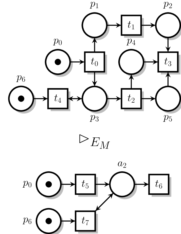
Figure 1: An example of Petri net, $M_{1}$ (top), and one of its polyhedral abstraction, $M_{2}$ (bottom), with $E_{M}\triangleq(p_{5}=p_{4}),(a_{1}=p_{1}+p_{2}),(a_{2}=p_{3}+p_{4}),(a_{1}=a_{2})$.

Given a marked net $(N,m_{0})$, we say that places $p,q$ of $N$ are concurrent when there exists a reachable marking $m$ with both $p$ and $q$ marked. The concurrent places problem consists in enumerating all such pairs of places.

Definition 3.2 (Dead and concurrent places).

We say that a place $p$ of $(N,m_{0})$ is nondead if there is $m$ in $R(N,m_{0})$ such that $m(p)>0$. Similarly, we say that places $p,q$ are concurrent, denoted $p\mathbin{\|}q$, if there is $m$ in $R(N,m_{0})$ such that both $m(p)>0$ and $m(q)>0$. By extension, we use the notation $p\mathbin{\|}p$ when $p$ is nondead. We say that $p,q$ are nonconcurrent, denoted $p\mathbin{\#}q$, when they are not concurrent.

Relation with linear arithmetic constraints

Many results in Petri net theory are based on a relation with linear algebra and linear programming techniques [24, 26]. A celebrated example is that the potentially reachable markings (an over-approximation of the reachable markings) of a net $(N,m_{0})$ are non-negative, integer solutions to the state equation problem, $m=I\cdot\sigma+m_{0}$, with $I$ an integer matrix defined from the flow functions of $N$ called the incidence matrix and $\sigma$ a vector in $\mathbb{N}^{k}$. It is known that solutions to the system of linear equations $\sigma^{T}\cdot I=\vec{0}$ lead to place invariants, $\sigma^{T}\cdot m=\sigma^{T}\cdot m_{0}$, that can provide some information on the decomposition of a net into blocks of nonconcurrent places, and therefore information on the concurrency relation.

For example, for net $M_{1}$ (Fig. 1), we can compute invariant $p_{4}-p_{5}=0$. This is enough to prove that places $p_{4}$ and $p_{5}$ are concurrent, if we can prove that at least one of them is nondead. Likewise, an invariant of the form $p+q=1$ is enough to prove that $p$ and $q$ are $1$-bounded and cannot be concurrent. Unfortunately, invariants provide only an over-approximation of the set of reachable markings, and it may be difficult to find whether a net is part of the few known classes where the set of reachable markings equals the set of potentially reachable ones [17].

Our approach shares some similarities with this kind of reasoning. A main difference is that we will use equation systems to draw a relation between the reachable markings of two nets; not to express constraints about (potentially) reachable markings inside one net. Like with invariants, this will allow us, in many cases, to retrieve information about the concurrency relation without “firing any transition”, that is without exploring the state space.

In the following, we will often use place names as variables, and markings $m:P\to\mathbb{N}$ as partial solutions to a set of linear equations. For the sake of simplicity, all our equations will be of the form $x=y_{1}+\dots+y_{l}$ or $y_{1}+\dots+y_{l}=k$ (with $k$ a constant in $\mathbb{N}$).

Given a system of linear equations $E$, we denote $\mathit{fv}({E})$ the set of all its variables. We are only interested in the non-negative integer solutions of $E$. Hence, in our case, a solution to $E$ is a total mapping from variables in $\mathit{fv}({E})$ to $\mathbb{N}$ such that all the equations in $E$ are satisfied. We say that $E$ is consistent when there is at least one such solution. Given these definitions, we say that the mapping $m:\{p_{1},\dots,p_{n}\}\to\mathbb{N}$ is a (partial) solution of $E$ if the system $E\mathbin{\raisebox{0.77498pt}{{,}}}\lfloor{m}\rfloor$ is consistent, where $\lfloor{m}\rfloor$ is the sequence of equations $p_{1}=m(p_{1})\mathbin{\raisebox{0.77498pt}{{,}}}\dots\mathbin{\raisebox{0.77498pt}{{,}}}p_{n}=m(p_{n})$. (In some sense, we use $\lfloor{m}\rfloor$ as a substitution.) For instance, places $p,q$ are concurrent if the system $p=1+x\mathbin{\raisebox{0.77498pt}{{,}}}q=1+y\mathbin{\raisebox{0.77498pt}{{,}}}\lfloor{m}\rfloor$ is consistent, where $m$ is a reachable marking and $x,y$ are some fresh (slack) variables.

Given two markings $m_{1}:P_{1}\to\mathbb{N}$ and $m_{2}:P_{2}\to\mathbb{N}$, from possibly different nets, we say that $m_{1}$ and $m_{2}$ are compatible, denoted $m_{1}\equiv m_{2}$, if they have equal marking on their shared places: $m_{1}(p)=m_{2}(p)$ for all $p$ in $P_{1}\cap P_{2}$. This is a necessary and sufficient condition for the system $\lfloor{m_{1}}\rfloor\mathbin{\raisebox{0.77498pt}{{,}}}\lfloor{m_{2}}\rfloor$ to be consistent.

4 Polyhedral abstraction

We recently defined a notion of polyhedral abstraction [1, 2] based on our previous work applying structural reductions to model counting [6, 7]. We only need a simplified version of this notion here, which entails an equivalence between the state space of two nets, $(N_{1},m_{1})$ and $(N_{2},m_{2})$, “up-to” a system $E$ of linear equations.

Definition 4.1 ($E$-equivalence).

We say that $(N_{1},m_{1})$ is $E$-equivalent to $(N_{2},m_{2})$, denoted $(N_{1},m_{1})\vartriangleright_{E}(N_{2},m_{2})$, if and only if:

(A1)

$E\mathbin{\raisebox{0.77498pt}{{,}}}\lfloor{m}\rfloor$ is consistent for all markings $m$ in $R(N_{1},m_{1})$ or $R(N_{2},m_{2})$;

(A2)

initial markings are compatible, meaning $E\mathbin{\raisebox{0.77498pt}{{,}}}\lfloor{m_{1}}\rfloor\mathbin{\raisebox{0.77498pt}{{,}}}\lfloor{m_{2}}\rfloor$ is consistent;

(A3)

assume $m^{\prime}_{1},m^{\prime}_{2}$ are markings of $N_{1},N_{2}$, respectively, such that $E\mathbin{\raisebox{0.77498pt}{{,}}}\lfloor{m^{\prime}_{1}}\rfloor\mathbin{\raisebox{0.77498pt}{{,}}}\lfloor{m^{\prime}_{2}}\rfloor$ is consistent, then $m^{\prime}_{1}$ is reachable if and only if $m^{\prime}_{2}$ is reachable:

$m^{\prime}_{1}\in R(N_{1},m_{1})\iff m_{2}^{\prime}\in R(N_{2},m_{2})$.

By definition, relation $\vartriangleright_{E}$ is symmetric. We deliberately use a symbol oriented from left to right to stress the fact that $N_{2}$ should be a reduced version of $N_{1}$. In particular, we expect to have fewer places in $N_{2}$ than in $N_{1}$.

Given a relation $(N_{1},m_{1})\vartriangleright_{E}(N_{2},m_{2})$, each marking $m^{\prime}_{2}$ reachable in $N_{2}$ can be associated to a unique subset of markings reachable in $N_{1}$, defined from the solutions to $E\mathbin{\raisebox{0.77498pt}{{,}}}\lfloor{m^{\prime}_{2}}\rfloor$ (by conditions (A1) and (A3)). We can show [1, 2] that this gives a partition of the reachable markings of $(N_{1},m_{1})$ into “convex sets”—hence the name polyhedral abstraction—each associated to a reachable marking in $N_{2}$. Our approach is particularly useful when the state space of $N_{2}$ is very small compared to the one of $N_{1}$. In the extreme case, we can even find examples where $N_{2}$ is the “empty” net (a net with zero places, and therefore a unique marking), but this condition is not a requisite in our approach.

We can illustrate this result using the two marked nets $M_{1},M_{2}$ in Fig. 1, for which we can prove that $M_{1}\vartriangleright_{E_{M}}M_{2}$ (detailed in [1, 2]). We have that $m^{\prime}_{2}\triangleq({p_{0}}={0}\mathbin{\raisebox{0.77498pt}{{,}}}{p_{6}}={1}\mathbin{\raisebox{0.77498pt}{{,}}}{a_{2}}={1})$ is reachable in $M_{2}$, which means that every solution to the system $p_{0}=0\mathbin{\raisebox{0.77498pt}{{,}}}p_{6}=1\mathbin{\raisebox{0.77498pt}{{,}}}p_{4}=p_{5}\mathbin{\raisebox{0.77498pt}{{,}}}p_{1}+p_{2}=1\mathbin{\raisebox{0.77498pt}{{,}}}p_{3}+p_{4}=1$ gives a reachable marking of $M_{1}$. Moreover, every solution such that $p_{i}\geqslant 1$ and $p_{j}\geqslant 1$ gives a witness that $p_{i}\mathbin{\|}p_{j}$. For instance, $p_{1},p_{4},p_{5}$ and $p_{6}$ are certainly concurrent together. We should exploit the fact that, under some assumptions about $E$, we can find all such “pairs of variables” without the need to explicitly solve systems of the form $E\mathbin{\raisebox{0.77498pt}{{,}}}\lfloor{m}\rfloor$; just by looking at the structure of $E$.

For this current work, we do not need to explain how to derive or check that an equivalence statement is correct in order to describe our method. In practice, we start from an initial net, $(N_{1},m_{1})$, and derive $(N_{2},m_{2})$ and $E$ using a combination of several structural reduction rules. You can find a precise description of our set of rules in [7] and a proof that the result of these reductions always leads to a valid $E$-equivalence in [1, 2]. The system of linear equations obtained using this process exhibits a graph-like structure. In the next section, we describe a set of constraints that formalizes this observation. This is one of the contributions of this paper, since we never defined something equivalent in our previous works. We show with our benchmarks (Sect. 9) that these constraints are general enough to give good results on a large set of models.

5 Token Flow Graphs

We introduce a set of structural constraints on the equations occurring in an equivalence statement $(N_{1},m_{1})\vartriangleright_{E}(N_{2},m_{2})$. The goal is to define an algorithm that is able to easily compute information on the concurrency relation of $N_{1}$, given the concurrency relation on $N_{2}$, by taking advantage of the structure of the equations in $E$.

We define the Token Flow Graph (TFG) of a system $E$ of linear equations as a Directed Acyclic Graph (DAG) with one vertex for each variable occurring in $E$. Arcs in the TFG are used to depict the relation induced by equations in $E$. We consider two kinds of arcs. Arcs for redundancy equations, $q\mathbin{{\rightarrow}\!{\bullet}}p$, to represent equations of the form $p=q$ (or $p=q+r+\dots$), expressing that the marking of place $p$ can be reconstructed from the marking of $q,r,\dots$ In this case, we say that place $p$ is removed by arc $q\mathbin{{\rightarrow}\!{\bullet}}p$, because the marking of $q$ may influence the marking of $p$, but not necessarily the other way round. Figure 2 illustrates such reduction rules on a subpart of the net $M_{1}$ given in Fig. 1. In this case, place $p_{4}$ has the same $\mathrm{Pre}$ and $\mathrm{Post}$ relation than $p_{5}$, thus both places are redundant. And so, by removing place $p_{5}$ we obtain the TFG on the right, corresponding to the equation $p_{5}=p_{4}$ (modeled by a “black dot” arc).

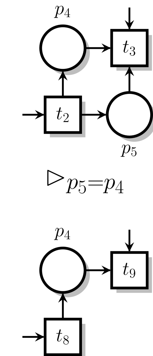
Figure 2: Redundancy reduction applied on a subpart of the net $M_{1}$ from Fig. 1 (left) and its corresponding TFG (right).

 

The second kind of arcs, $a\mathbin{{\circ}\!{\rightarrow}}p$, is for agglomeration equations. It represents equations of the form $a=p+q$, generated when we agglomerate several places into a new one. In this case, we expect that if we can reach a marking with $k$ tokens in $a$, then we can certainly reach a marking with $k_{1}$ tokens in $p$ and $k_{2}$ tokens in $q$ when $k=k_{1}+k_{2}$ (see property Agglomeration in Lemma 6.2). Hence, the marking of $p$ and $q$ can be reconstructed from the marking of $a$. Thus, we say that places p and q are removed. We also say that node $a$ is inserted; it does not exist in $N_{1}$ but may appear as a new place in $N_{2}$ unless it is removed by a subsequent reduction. We can have more than two places in an agglomeration. Figure 3 illustrates an example of such reduction obtained by agglomerating places $p_{1},p_{2}$ together, in net $M_{1}$ of Fig. 1, into a new place $a_{1}$. Thus, the TFG in Fig 3 (right) depicts the obtained equation $a_{1}=p_{1}+p_{2}$ (modeled by “white dot” arcs).

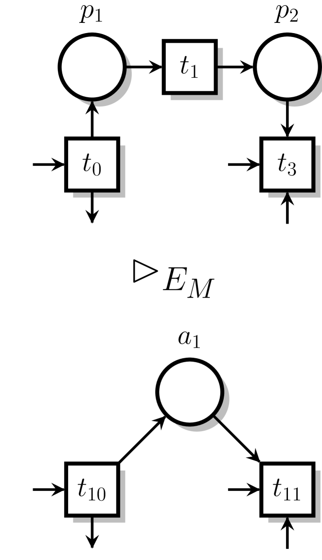
Figure 3: Agglomeration reduction applied on a subpart of the net $M_{1}$ from Fig. 1 (left) and its corresponding TFG (right).

 

A TFG can also include nodes for constants, used to express invariant statements on the markings of the form $p+q=k$. To this end, we assume that we have a family of disjoint sets $K(n)$ (also disjoint from place and variable names), for each $n$ in $\mathbb{N}$, such that the “valuation” of a node $v\in K(n)$ will always be $n$. We use $K$ to denote the set of all constants. We may write $v^{n}$ (instead of just $v$) for a constant node whose value is $n$.

Definition 5.1 (Token Flow Graph).

A TFG with set of places $P$ is a directed (bi)graph $(V,R,A)$ such that:

• $V=P\cup S$ is a set of vertices (or nodes) with $S\subset K$ a finite set of constants,

• $R\in V\times V$ is a set of redundancy arcs, $v\mathbin{{\rightarrow}\!{\bullet}}v^{\prime}$,

• $A\in V\times V$ is a set of agglomeration arcs, $v\mathbin{{\circ}\!{\rightarrow}}v^{\prime}$, disjoint from $R$.

The main source of complexity in our approach arises from the need to manage interdependencies between $A$ and $R$ arcs, that is situations where redundancies and agglomerations are combined. This is not something that can be easily achieved by looking only at the equations in $E$ and thus motivates the need for a specific data-structure.

We define several notations that will be useful in the following. We use the notation $v\rightarrow v^{\prime}$ when we have $(v\mathbin{{\rightarrow}\!{\bullet}}v^{\prime})$ in $R$ or $(v\mathbin{{\circ}\!{\rightarrow}}v^{\prime})$ in $A$. We say that a node $v$ is a root if it is not the target of an arc. It is a $\circ$-leaf when it has no output arc of the form $(v\mathbin{{\circ}\!{\rightarrow}}v^{\prime})$. A sequence of nodes $(v_{1},\dots,v_{n})$ in $V^{n}$ is a path if for all $1\leqslant i<n$ we have $v_{i}\rightarrow v_{i+1}$. We use the notation $v\rightarrow^{\star}v^{\prime}$ when there is a path from $v$ to $v^{\prime}$ in the graph, or when $v=v^{\prime}$. We write $v\mathbin{{\circ}\!{\rightarrow}}X$ when $X$ is the largest subset $\{v_{1},\dots,v_{k}\}$ of $V$ such that $X\neq\emptyset$ and for all $i\in 1..k$, $v\mathbin{{\circ}\!{\rightarrow}}v_{i}\in A$. Similarly, we write $X\mathbin{{\rightarrow}\!{\bullet}}v$ when $X$ is the largest, non-empty set of nodes $\{v_{1},\dots,v_{k}\}$ such that for all $i\in 1..k$, $v_{i}\mathbin{{\rightarrow}\!{\bullet}}v\in R$. Finally, the notation $\mathord{\downarrow}{v}$ denotes the set of successors of $v$, that is: $\mathord{\downarrow}{v}\triangleq\{v^{\prime}\in V\,\mid\,v\rightarrow^{\star}v^{\prime}\}$.

We display an example of Token Flow Graphs in Fig. 4, where “black dot” arcs model edges in $R$ and “white dot” arcs model edges in $A$. The idea is that each relation $X\mathbin{{\rightarrow}\!{\bullet}}v$ or $v\mathbin{{\circ}\!{\rightarrow}}X$ corresponds to one equation $v=\sum_{v_{i}\in X}v_{i}$ in $E$, and that all the equations in $E$ should be reflected in the TFG. We want to avoid situations where the same place is removed more than once, or where some place occurs in the TFG but is never mentioned in $N_{1},N_{2}$ or $E$. We also have the roots (without eventual constant nodes) that match to the places in $N_{2}$, and the $\mathbin{{\circ}\!{\rightarrow}}$-leaves to the places in $N_{1}$. All these constraints can be expressed using a suitable notion of well-formed graph.

Definition 5.2 (Well-formed TFG).

A TFG $G=(V,R,A)$ for the equivalence statement $(N_{1},m_{1})\vartriangleright_{E}(N_{2},m_{2})$ is well-formed when all the following constraints are met, where $P_{1}$ and $P_{2}$ stand for the set of places in $N_{1}$ and $N_{2}$:

(T1)

no unused names: $V\setminus K=P_{1}\cup P_{2}\cup\mathit{fv}({E})$;

(T2)

nodes in $K$ are roots: if $v\in V\cap K$ then $v$ is a root of $G$;

(T3)

nodes can be removed only once: it is not possible to have $p\mathbin{{\circ}\!{\rightarrow}}q$ and $p^{\prime}\rightarrow q$ with $p\neq p^{\prime}$, or to have both $p\mathbin{{\rightarrow}\!{\bullet}}q$ and $p\mathbin{{\circ}\!{\rightarrow}}q$;

(T4)

we have all and only the equations in $E$: we have $v\mathbin{{\circ}\!{\rightarrow}}X$ or $X\mathbin{{\rightarrow}\!{\bullet}}v$ if and only if the equation $v=\sum_{v_{i}\in X}v_{i}$ is in $E$;

(T5)

$G$ is acyclic;

(T6)

nodes in $G$ match nets: the set of roots of $G$, without constants $K$, equals the set $P_{2}$. The set of $\circ$-leaves of $G$, without constants $K$, equals the set $P_{1}$.

Given a relation $(N_{1},m_{1})\vartriangleright_{E}(N_{2},m_{2})$, the well-formedness conditions are enough to ensure the unicity of a TFG (up-to the choice of constant nodes) when we set each equation to be either in $A$ or in $R$. In this case, we denote this TFG $\llbracket{E}\rrbracket$. In practice, we use a tool called Reduce to generate the $E$-equivalence from the initial net $(N_{1},m_{1})$. This tool outputs a sequence of equations suitable to build a TFG and, for each equation, it adds a tag indicating if it is a Redundancy or an Agglomeration. We display in Fig. 4 the equations generated by Reduce for the net $M_{1}$ given in Fig. 1.

    # R |- p5 = p4
    # A |- a1 = p2 + p1
    # A |- a2 = p4 + p3
    # R |- a1 = a2
    

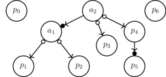
Figure 4: Equations generated from net $M_{1}$, in Fig. 1, and their associated TFG.

The constraints (T1)–(T6) are not artificial or arbitrary. In practice, we compute $E$-equivalences using multiple steps of structural reductions, and a TFG exactly records the constraints and information generated during these reductions. In some sense, equations $E$ abstract a relation between the semantics of two nets, whereas a TFG records the structure of reductions between places.

6 Semantics

By construction, there is a strong connection between “systems of reduction equations”, $E$, and their associated graph, $\llbracket{E}\rrbracket$. We show that a similar relation exists between solutions of $E$ and “valuations” of the graph (which we call configurations thereafter).

A configuration $c$ of a TFG $(V,R,A)$ is a partial function from $V$ to $\mathbb{N}$. We use the notation $c(v)=\bot$ when $c$ is not defined on $v$, and we always assume that $c(v)=n$ when $v$ is a constant node in $K(n)$.

Configuration $c$ is total when $c(v)$ is defined for all nodes $v$ in $V$; otherwise it is said partial. We use the notation $c_{\mid N}$ for the configuration obtained from $c$ by restricting its domain to the set of places in the net $N$. We remark that when $c$ is defined over all places of $N$ then $c_{\mid N}$ can be viewed as a marking. As for markings, we say that two configurations $c$ and $c^{\prime}$ are compatible, denoted $c\equiv c^{\prime}$, if they have same value on the nodes where they are both defined: $c(p)=c^{\prime}(p)$ when $c(v)\neq\bot$ and $c^{\prime}(v)\neq\bot$. (Same holds when comparing a configuration to a marking.) We also use $\lfloor{c}\rfloor$ to represent the system $v_{1}=c(v_{1})\mathbin{\raisebox{0.77498pt}{{,}}}\dots\mathbin{\raisebox{0.77498pt}{{,}}}v_{k}=c(v_{k})$ where the $(v_{i})_{i\in 1..k}$ are the nodes such that $c(v_{i})\neq\bot$. We say that a configuration $c$ is well-defined when the valuation of the nodes agrees with the equations of $\llbracket{E}\rrbracket$.

Definition 6.1 (Well-defined configuration).

Configuration $c$ is well-defined when for all nodes $p$ the following two conditions hold:

(CBot)

if $v\rightarrow w$ then $c(v)=\bot$ if and only if $c(w)=\bot$;

(CEq)

if $c(v)\neq\bot$ and $v\mathbin{{\circ}\!{\rightarrow}}X$ or $X\mathbin{{\rightarrow}\!{\bullet}}v$ then $c(v)=\sum_{v_{i}\in X}c(v_{i})$.

We prove that the well-defined configurations of a TFG $\llbracket{E}\rrbracket$ are partial solutions of $E$, and reciprocally. Therefore, because all the variables in $E$ are nodes in the TFG (condition (T1)) we have an equivalence between solutions of $E$ and total, well-defined configurations of $\llbracket{E}\rrbracket$.

Lemma 6.1 (Well-defined configurations are solutions).

Assume $\llbracket{E}\rrbracket$ is a well-formed TFG for the equivalence $(N_{1},m_{1})\vartriangleright_{E}(N_{2},m_{2})$. If $c$ is a well-defined configuration of $\llbracket{E}\rrbracket$ then $E\mathbin{\raisebox{0.77498pt}{{,}}}\lfloor{c}\rfloor$ is consistent. Conversely, if $c$ is a total configuration of $\llbracket{E}\rrbracket$ such that $E\mathbin{\raisebox{0.77498pt}{{,}}}\lfloor{c}\rfloor$ is consistent then $c$ is also well-defined.

Proof: We prove each property separately.

Assume $c$ is a well-defined configuration of $\llbracket{E}\rrbracket$. Since $E$ is a system of reduction equations, it is a sequence of equalities $\phi_{1},\dots,\phi_{k}$ where each equation $\phi_{i}$ has the form $x_{i}=y_{1}+\dots+y_{n}$. Also, since $\llbracket{E}\rrbracket$ is well-formed we have that $X_{i}\mathbin{{\rightarrow}\!{\bullet}}v_{i}$ or $x_{i}\mathbin{{\circ}\!{\rightarrow}}X_{i}$ (only one case is possible) with $X_{i}=\{y_{1},\dots,y_{n}\}$ for all indices $i\in 1..k$. We define $I$ the subset of indices in $1..k$ such that $c(x_{i})$ is defined. By condition (CBot) we have $c(x_{i})\neq\bot$ if and only if $c(v)\neq\bot$ for all $v\in X_{i}$. Therefore, if $c(x_{i})\neq\bot$, we have by condition (CEq) that $\phi_{i}\mathbin{\raisebox{0.77498pt}{{,}}}\lfloor{c}\rfloor$ is consistent. Moreover, the values of all the variables in $\phi_{i}$ are determined by $\lfloor{c}\rfloor$ (these variables have the same value in every solution). As a consequence, the system combining $\lfloor{c}\rfloor$ and the $(\phi_{i})_{i\in I}$ has a unique solution. On the opposite, if $c(x_{i})=\bot$ then no variables in $\phi_{i}$ are defined by $\lfloor{c}\rfloor$. Nonetheless, we know that system $E$ is consistent. Indeed, by property of $E$-equivalence, we know that $E\mathbin{\raisebox{0.77498pt}{{,}}}\lfloor{m_{1}}\rfloor$ has solutions, so it is also the case with $E$. Therefore, the system combining the equations in $(\phi_{i})_{i\notin I}$ is consistent. Since this system shares no variables with the equations in $(\phi_{i})_{i\in I}$, we have that $E\mathbin{\raisebox{0.77498pt}{{,}}}\lfloor{c}\rfloor$ is consistent.

For the second case, we assume $c$ total and $E\mathbin{\raisebox{0.77498pt}{{,}}}\lfloor{c}\rfloor$ consistent. Since $c$ is total, condition (CBot) is true ($c(v)\neq\bot$ for all nodes in $\llbracket{E}\rrbracket$). Assume we have $(N_{1},m_{1})\vartriangleright_{E}(N_{2},m_{2})$. For condition (CEq), we rely on the fact that $\llbracket{E}\rrbracket$ is well-formed (T4). Indeed, for all equations in $E$ we have a corresponding relation $X\mathbin{{\rightarrow}\!{\bullet}}v$ or $v\mathbin{{\circ}\!{\rightarrow}}X$. Hence $E\mathbin{\raisebox{0.77498pt}{{,}}}\lfloor{c}\rfloor$ consistent implies that $c(v)=\sum_{w\in X}c(w)$.

We can prove several properties related to how the structure of a TFG constrains possible values in well-defined configurations. These results can be thought of as the equivalent of a “token game”, which explains how tokens can propagate along the arcs of a TFG. This is useful in our context since we can assess that two nodes are concurrent when we can mark them in the same configuration. (A similar result holds for finding pairs of nonconcurrent nodes.)

Our first result shows that we can always propagate tokens from a node to its children, meaning that if a node has a token, we can find one in its successors (possibly in a different well-defined configuration). Property (Backward) states a dual result; if a child node is marked then one of its parents must be marked.

Lemma 6.2 (Token propagation).

Assume $\llbracket{E}\rrbracket$ is a well-formed TFG for the equivalence $(N_{1},m_{1})\vartriangleright_{E}(N_{2},m_{2})$ and $c$ a well-defined configuration of $\llbracket{E}\rrbracket$.

(Agglomeration)

if $p\mathbin{{\circ}\!{\rightarrow}}\{q_{1},\dots,q_{k}\}$ and $c(p)\neq\bot$ then for every sequence $(l_{i})_{i\in 1..k}$ of $\mathbb{N}^{k}$ such that $c(p)=\sum_{i\in 1..k}l_{i}$, we can find a well-defined configuration $c^{\prime}$ such that $c^{\prime}(p)=c(p)$, and $c^{\prime}(q_{i})=l_{i}$ for all $i\in 1..k$, and $c^{\prime}(v)=c(v)$ for every node $v$ not in $\mathord{\downarrow}{p}$.

(Forward)

if $p,q$ are nodes such that $c(p)\neq\bot$ and $p\rightarrow^{\star}q$ then we can find a well-defined configuration $c^{\prime}$ such that $c^{\prime}(q)\geqslant c^{\prime}(p)=c(p)$ and $c^{\prime}(v)=c(v)$ for every node $v$ not in $\mathord{\downarrow}{p}$.

(Backward)

if $c(p)>0$ then there is a root $v$ such that $v\rightarrow^{\star}p$ and $c(v)>0$.

Proof: We prove each property separately. Without loss of generality, we assume there exists an (arbitrary) total ordering on nodes.

Agglomeration: let $p$ be a node such that $p\mathbin{{\circ}\!{\rightarrow}}X$, with $X=\{q_{1},\dots,q_{k}\}$, and let $(l_{1},\dots,l_{k})\in\mathbb{N}^{k}$ be a sequence such that $c(p)=\sum_{i\in 1..k}l_{i}$. We define configuration $c^{\prime}$ as a recursive function. The base cases are defined by: $c^{\prime}(p)=c(p)$, for all $i\in 1..k$, $c^{\prime}(q_{i})=l_{i}$, and $c^{\prime}(v)=c(v)$ for all the nodes $v$ such that $v\notin\mathord{\downarrow}{p}$. The recursive cases concern only the nodes that are successors of nodes in $X$. Let $w$ be such a node. It cannot be a root (since $w$ is a successor of a node in $X$), hence it has at least one parent $x$. We consider two cases:

• Either $x\mathbin{{\rightarrow}\!{\bullet}}w$ holds: then, let $Y$ be the set of parents of $w$ (as expected, $x\in Y$). Property (T3) of Definition 5.2 implies that $Y\mathbin{{\rightarrow}\!{\bullet}}w$ holds, and we define $c^{\prime}(w)=\sum_{y\in Y}c^{\prime}(y)$.

• Or $x\mathbin{{\circ}\!{\rightarrow}}w$ holds: then $x$ is the only parent of $w$ by property (T3). Let $Y$ be the set of agglomeration children of $x$: we have $x\mathbin{{\circ}\!{\rightarrow}}Y$, and $w\in Y$. We define $c^{\prime}(w)=c^{\prime}(x)$ if $w$ is the smallest node of $Y$ (according to the total ordering on nodes), or $c^{\prime}(w)=0$ otherwise. This entails $c^{\prime}(x)=\sum_{y\in Y}c^{\prime}(y)$ (where all terms are defined as zero except one defined as $c^{\prime}(x)$).

Note that the recursion always implies the parents of a given node, and is therefore well-founded since a TFG is a DAG. It is immediate to check that $c^{\prime}$ is well-defined: by construction, (CEq) is satisfied on all nodes where $c^{\prime}$ is defined.

Forward: take a well-defined configuration $c$ of $\llbracket{E}\rrbracket$ and assume we have two nodes $p,q$ such that $c(p)\neq\bot$ and $p\rightarrow^{\star}q$. The proof is by induction on the length of the path from $p$ to $q$. The initial case is when $p=q$, which is trivial. Otherwise, assume $p\rightarrow r\rightarrow^{\star}q$. It is enough to find a well-defined configuration $c^{\prime}$ such that $c^{\prime}(r)\geqslant c^{\prime}(p)=c(p)$. Since the nodes not in $\mathord{\downarrow}{p}$ are not in the paths from $p$ to $q$, we can ensure $c^{\prime}(v)=c(v)$ for any node $v$ not in $\mathord{\downarrow}{p}$. The proof proceeds by a case analysis on $p\rightarrow r$:

• Either $X\mathbin{{\rightarrow}\!{\bullet}}r$ with $p\in X$. Then by (CEq) we have $c(r)=c(p)+\sum_{v\in X,v\neq p}c(v)\geqslant c(p)$ and we can choose $c^{\prime}=c$.

• Or we have $p\mathbin{{\circ}\!{\rightarrow}}X$ with $r\in X$. By (Agglomeration) we can find a well-defined configuration $c^{\prime}$ such that $c^{\prime}(r)=c^{\prime}(p)=c(p)$ (and also $c^{\prime}(v)=0$ for all $v\in X\setminus\{r\}$).

Backward: let $c$ be a well-defined configuration of $\llbracket{E}\rrbracket$ and assume we have $c(p)>0$. The proof is by reverse structural induction on the DAG. If $p$ is a root, the result is immediate ; otherwise, $p$ has at least one parent $q$ such that $q\rightarrow p$. As above, we proceed by case analysis.

• Either $X\mathbin{{\rightarrow}\!{\bullet}}p$ with $q\in X$. By (CEq), we have $c(p)=\sum_{v\in X}c(v)>0$. Hence there must be at least one node $q^{\prime}$ in $X$ such that $c(q^{\prime})>0$ and we conclude by induction hypothesis on $q^{\prime}$, which is a parent of $p$.

• Or we have $q\mathbin{{\circ}\!{\rightarrow}}X$ with $p\in X$. By (CEq), we have $c(q)=\sum_{v\in X}c(v)\geqslant c(p)>0$, and we conclude by induction hypothesis on $q$, which is again a parent of $p$.

Until this point, none of our results rely on the properties of $E$-equivalence. We now prove that there is an equivalence between the reachable markings –of $N_{1}$ and $N_{2}$– and configurations of $\llbracket{E}\rrbracket$. More precisely, we prove (Theorem 6.3) that every reachable marking in $N_{1}$ or $N_{2}$ can be extended into a well-defined configuration of $\llbracket{E}\rrbracket$. This entails that we can reconstruct all the reachable markings of $N_{1}$ by looking at well-defined configurations obtained from the reachable markings of $N_{2}$. Our algorithm for computing the concurrency relation (see Sect. 8) will be a bit smarter since we do not need to enumerate exhaustively all the markings of $N_{2}$. Instead, we only need to know which roots can be marked together.

Theorem 6.3 (Configuration reachability).

Assume $\llbracket{E}\rrbracket$ is a well-formed TFG for the equivalence $(N_{1},m_{1})\vartriangleright_{E}(N_{2},m_{2})$. If $m$ is a marking in $R(N_{1},m_{1})$ or $R(N_{2},m_{2})$ then there exists a total, well-defined configuration $c$ of $\llbracket{E}\rrbracket$ such that $c\equiv m$. Conversely, given a total, well-defined configuration $c$ of $\llbracket{E}\rrbracket$, marking $c_{\mid N_{1}}$ is reachable in $(N_{1},m_{1})$ if and only if $c_{\mid N_{2}}$ is reachable in $(N_{2},m_{2})$.

Proof: We prove each point separately.

First, we take a marking $m$ in $R(N_{1},m_{1})$ (the case $m$ in $R(N_{2},m_{2})$ is similar). By property (A1) of Definition 4.1, $E\mathbin{\raisebox{0.77498pt}{{,}}}\lfloor{m}\rfloor$ is consistent. Hence, it admits a non-negative integer solution $c$, meaning a valuation for all the variables and places in $\mathit{fv}({E}),N_{1}$ and $N_{2}$ such that $E\mathbin{\raisebox{0.77498pt}{{,}}}\lfloor{c}\rfloor$ is consistent and $c(p)=m(p)$ if $p\in N_{1}$. We may freely extend $c$ to include constants in $K$ (whose values are fixed), thus according to condition (T1) of Definition 5.2, this solution $c$ is defined over all the nodes of $\llbracket{E}\rrbracket$. It is well-defined by virtue of Lemma 6.1.

For the converse property, we assume that $c$ is a total, well-defined configuration of $\llbracket{E}\rrbracket$ and that $c_{\mid N_{1}}$ is in $R(N_{1},m_{1})$ (the case $c_{\mid N_{2}}$ in $R(N_{2},m_{2})$ is again similar). Since $c$ is a well-defined configuration, from Lemma 6.1 we have that $E\mathbin{\raisebox{0.77498pt}{{,}}}\lfloor{c}\rfloor$ is consistent. Therefore we have that $E\mathbin{\raisebox{0.77498pt}{{,}}}\lfloor{c_{\mid N_{1}}}\rfloor\mathbin{\raisebox{0.77498pt}{{,}}}\lfloor{c_{\mid N_{2}}}\rfloor$ is consistent. By condition (A3) of Definition 4.1, we have $c_{\mid N_{2}}$ in $R(N_{2},m_{2})$, as needed.

The second result of this theorem justifies the following definition.

Definition 6.2 (Reachable configuration).

Configuration $c$ is reachable for an equivalence statement $(N_{1},m_{1})\vartriangleright_{E}(N_{2},m_{2})$ if $c$ is total, well-defined and $c_{\mid N_{1}}\in R(N_{1},m_{1})$ (resp. $c_{\mid N_{2}}\in R(N_{2},m_{2})$).

The previous fundamental results demonstrate the possibilities of TFGs to reason about the state space of the initial net from the one of the reduced net, and vice versa.

7 Marking reachability

We illustrate the benefit of Token Flow Graphs by describing a simple model-checking algorithm. The goal is to decide if a marking, say $m_{1}^{\prime}$, is reachable in the initial net $(N_{1},m_{1})$, by checking a reachability property on the smaller net $(N_{2},m_{2})$. We start by proving some auxiliary results.

Lemma 7.1 (Unicity of marking reduction).

Assume $\llbracket{E}\rrbracket$ is a well-formed TFG for the equivalence $(N_{1},m_{1})\vartriangleright_{E}(N_{2},m_{2})$. Given a marking $m_{1}^{\prime}$ of $N_{1}$ there exists at most one total, well-defined configuration $c$ such that $c\equiv m_{1}^{\prime}$.

Proof: Let $c_{1}$ and $c_{2}$ be two total, well-defined configurations such that $c_{1}\equiv m_{1}^{\prime}$ and $c_{2}\equiv m_{1}^{\prime}$. Let $X$ be the set of nodes $x$ such that $c_{1}(x)\neq c_{2}(x)$. By contradiction, we assume $X$ is not empty (that is, we assume $c_{1}\neq c_{2}$). For each node $x$ in $X$, we know that $x$ does not belong to $P_{1}$, since $c_{1}$ and $c_{2}$ agree on $m_{1}^{\prime}$. Consequently, by virtue of property (T6) of Definition 5.2, each $x$ in $X$ admits an output $x\mathbin{{\circ}\!{\rightarrow}}y$. More generally, for each $x$ in $X$, we have $x\mathbin{{\circ}\!{\rightarrow}}Y$ for some non-empty set $Y$. We consider an element $x_{0}$ of $X$ such that $x_{0}\mathbin{{\circ}\!{\rightarrow}}Y_{0}$ holds with $Y_{0}$ disjoint from $X$ (such an element $x_{0}$ necessarily exists if $X$ is not empty, otherwise $X$ would contain a cycle of $\circ$-arcs, which is forbidden by the acyclic property (T5) of the well-formed TFG). Then, since $c_{1}$ is well-defined, we know that $c_{1}(x_{0})=\sum_{y\in Y_{0}}c_{1}(y)$ by property (CEq). However, we have $c_{1}(y)=c_{2}(y)$ for all $y\in Y_{0}$ since $Y_{0}$ is disjoint from $X$. Hence, $c_{1}(x_{0})=\sum_{y\in Y_{0}}c_{2}(y)=c_{2}(x_{0})$, which contradicts $x_{0}\in X$. As a conclusion, $X$ must be empty, that is $c_{1}=c_{2}$. There can be at most one well-defined configuration.

Then, as a corollary of this lemma and of Theorem 6.3, we get:

Theorem 7.2 (Reachability decision).

Assume $\llbracket{E}\rrbracket$ is a well-formed TFG for the equivalence $(N_{1},m_{1})\vartriangleright_{E}(N_{2},m_{2})$. Deciding if a marking $m^{\prime}_{1}$ is reachable in $R(N_{1},m_{1})$ amounts to construct a total, well-defined configuration $c$ such that $c\equiv m^{\prime}_{1}$ and then check if $c_{\mid N_{2}}$ is reachable in $R(N_{2},m_{2})$.

Hence, given an equivalence $(N_{1},m_{1})\vartriangleright_{E}(N_{2},m_{2})$ and the associated TFG $\llbracket{E}\rrbracket$, we first extend our marking of interest $m_{1}^{\prime}$ into a total well-defined configuration $c$, as done by Algorithm 1, next. (Lemma 7.1 ensures that if such configuration exists, then it is unique.) As stated in Theorem 7.2, if $c$ restricted to $N_{2}$ is a marking reachable in $(N_{2},m_{2})$, then $m_{1}^{\prime}$ is reachable in $(N_{1},m_{1})$. Otherwise, $\neg\lfloor{m_{1}^{\prime}}\rfloor$ is an invariant on $R(N_{1},m_{1})$.

We illustrate this algorithm by taking two concrete examples on the marked net $M_{1}$ given in Fig. 1. Assume we want to decide if marking $m_{1}^{\prime}\triangleq({p_{0}}={0}\mathbin{\raisebox{0.77498pt}{{,}}}{p_{1}}={2}\mathbin{\raisebox{0.77498pt}{{,}}}{p_{2}}={0}\mathbin{\raisebox{0.77498pt}{{,}}}{p_{3}}={1}\mathbin{\raisebox{0.77498pt}{{,}}}{p_{4}}={1}\mathbin{\raisebox{0.77498pt}{{,}}}{p_{5}}={1}\mathbin{\raisebox{0.77498pt}{{,}}}{p_{6}}={0})$ is reachable in $(N_{1},m_{1})$, for $m_{1}$ as depicted in Fig. 1. This marking can be extended into a total, well-defined configuration $c$, with $c(a_{1})=c(a_{2})=2$. And so, deciding of the reachability of marking $m_{1}^{\prime}$ in $(N_{1},m_{1})$ is equivalent to decide if marking $m_{2}^{\prime}\triangleq({p_{0}}={0}\mathbin{\raisebox{0.77498pt}{{,}}}{a_{2}}={2}\mathbin{\raisebox{0.77498pt}{{,}}}{p_{6}}={0})$ is reachable in $(N_{2},m_{2}^{\prime})$ (which it is not). Observe that $m_{1}^{\prime}$ would be reachable if the initial marking $m_{1}$ was $({p_{0}}=2,{p_{6}}=1)$ and the other places empty. Conversely, assume our marking of interest is $m_{1}^{\prime\prime}$ such that $m_{1}^{\prime\prime}(p_{4})=2$ and $m_{1}^{\prime\prime}(p_{1})=m_{1}^{\prime\prime}(p_{2})=0$. It is not possible to extend this marking into a well-defined configuration $c$, since $c(a_{1})=m_{1}^{\prime\prime}(p_{1})+m_{1}^{\prime\prime}(p_{2})=0$ and $c(a_{1})=c(a_{2})>m_{1}^{\prime\prime}(p_{4})$. In this case, we directly obtain that $m_{1}^{\prime\prime}$ is not reachable in $(N_{1},m_{1})$, for every initial marking $m_{1}$.

The Reachable function (see Algorithm 1) is a direct implementation of Theorem 7.2: it builds a total configuration $c$, then checks that it is well-defined (we omit the function well-defined, which is obvious), and finally finds out if $c_{\mid N_{2}}$ is reachable in $(N_{2},m_{2})$. This algorithm relies on the recursive procedure BottomUp (see Algorithm 2) which extends the marking of interest $m_{1}^{\prime}$ into a total, well-defined configuration if there is one.

Algorithm 1 Reachable($m_{1}^{\prime}$, $\llbracket{E}\rrbracket$, $(N_{2},m_{2})$)

1:In:

$m_{1}^{\prime}$	:	a marking of $N_{1}$
$(N_{2},m_{2})$	:	reduced net such that
		$(N_{1},m_{1})\vartriangleright_{E}(N_{2},m_{2})$ holds
$\llbracket{E}\rrbracket$	:	well-formed TFG for
		the $E$-equivalence above

Out: a boolean indicating if $m_{1}^{\prime}\in R(N_{1},m_{1})$

2:$c\leftarrow\vec{\bot}$ ;; c is a configuration for $\llbracket{E}\rrbracket$

3:for all $p\in P_{1}$ do $c[p]\leftarrow m_{1}[p]$

4:for all $v^{n}\in K$ do $c[v]\leftarrow n$

5:;; $\llbracket{E}\rrbracket$ is $(V,R,A)$, as in Definition 5.1

6:for all $v\in V$ do BottomUp$(c,v,\llbracket{E}\rrbracket)$

7:return well-defined$(c)\land c_{\mid N_{2}}\in R(N_{2},m_{2})$

Algorithm 2 BottomUp($c,v,\llbracket{E}\rrbracket$)

1:

In:	$\llbracket{E}\rrbracket$ : the TFG structure
	$v$, a node in $\llbracket{E}\rrbracket$
In out:	$c$, a partial configuration of $\llbracket{E}\rrbracket$
Post:	$c$ is defined for all nodes of $\mathord{\downarrow}{v}$

2:for all $v^{\prime}$ such that $v\rightarrow v^{\prime}$ do

3:    BottomUp$(c,v^{\prime},\llbracket{E}\rrbracket)$

4:end for

5:if $v\mathbin{{\circ}\!{\rightarrow}}X$ then $c[v]\leftarrow\sum_{v^{\prime}\in X}c[v^{\prime}]$

We note that the second algorithm, which is recursive, always terminates since it simply follows the TFG structure. We still have to prove that Algorithm 1 always returns the correct answer.

Proof: We consider two cases:

• Case C1: the algorithm returns false because $c$ is not well-defined (line 7). In this case we show, next, that no well-defined configuration $c$ extending $m^{\prime}_{1}$ exists, and thus $m^{\prime}_{1}$ is not reachable by Theorem 6.3.

• Case C2: the algorithm returns the value of $c_{\mid N_{2}}\in R(N_{2},m_{2})$. In this case, thanks to Theorem 7.2, it suffices to show that $c$ is total, well-defined, and extends $m^{\prime}_{1}$.

We start by case C2, which basically states the soundness of the algorithm. Let us show that $c$ is total: for every node $v$, if $v$ is a constant, or if it belongs to $P_{1}$, it is set by lines 3 and 4 of Algorithm 1. Otherwise, $v$ is not a $\circ$-leaf (by property (T6) of Definition 5.2), hence it is set by line 5 of Algorithm 2, which is invoked on every node of the TFG (line 6, Algorithm 1). Additionally, $c$ is well-defined, because it passed the test line 7. It also extends $m^{\prime}_{1}$ by consequence of line 3 (those values are not overwritten later in Algorithm 2, because of property (T6)).

Case C1 states the completeness of the algorithm. By contraposition, we assume there exists a total well-defined configuration $c^{\prime}$ extending $m^{\prime}_{1}$, and show by induction on the recursive calls to BottomUp, that the algorithm builds a configuration $c$ equal to $c^{\prime}$. More precisely, we show that an invocation of $BottomUp(c,v,\llbracket{E}\rrbracket)$ returns a configuration $c$ that coincides with $c^{\prime}$ on all nodes of $\mathord{\downarrow}{v}$. The initial configuration $c$ built by the algorithm extends $m^{\prime}_{1}$ and sets the constants (lines 3 and 4 of Algorithm 1). Then, for any invocation of $BottomUp(c,v,\llbracket{E}\rrbracket)$, for every node $w$ in $\mathord{\downarrow}{v}$, if $w$ is a node in $P_{1}$, then $c(v)=c^{\prime}(v)$ holds immediately. Otherwise, $w$ is not a $\circ$-leaf. If $w\neq v$, then $w$ is in $\mathord{\downarrow}{u}$ for some child $u$ of $v$, and $c(v)=c^{\prime}(v)$ holds by induction hypothesis on the recursive call to $BottomUp(c,u,\llbracket{E}\rrbracket)$ that occurred on line 3. If $w=v$, then $c(v)$ is set by line 5, that is $c(v)=\sum_{v^{\prime}\in X}c(v^{\prime})$. By induction hypothesis, we have $c(v^{\prime})=c^{\prime}(v^{\prime})$ for all $v^{\prime}$ children of $v$ (the recursive call occurred also on line 3). Hence, $c(v)=\sum_{v^{\prime}\in X}c^{\prime}(v^{\prime})=c^{\prime}(v)$ by property (Ceq) since $c^{\prime}$ is well-defined. Consequently, $c(w)=c^{\prime}(w)$ for all $w$ in $\mathord{\downarrow}{v}$. As a result, $c=c^{\prime}$, since BottomUp is invoked on all nodes of the TFG.

State space partition

We can use the previous results to derive an interesting result about the state space of equivalent Petri nets, in the case where the associated TFG is well-formed. Indeed, we can prove that, in this case, we can build a partition of the reachable markings of $(N_{1},m_{1})$ that is in bijection with the reachable markings of $(N_{2},m_{2})$.

Given a marking $m_{2}^{\prime}$ of the reduced net $N_{2}$ we define $Inv(m_{2}^{\prime})$ as the set of markings of the initial net $N_{1}$ which are in relation with $m^{\prime}_{2}$.

$$Inv(m_{2}^{\prime})\triangleq\{c_{\mid N_{1}}\mid c\text{ total, well-defined }\land c\equiv m_{2}^{\prime}\}$$

Theorem 7.3 (State space partition).

Assume $\llbracket{E}\rrbracket$ is a well-formed TFG for the equivalence $(N_{1},m_{1})\vartriangleright_{E}(N_{2},m_{2})$. The family of sets $P\triangleq\{Inv(m_{2}^{\prime})\mid m_{2}^{\prime}\in R(N_{2},m_{2})\}$ is a partition of $R(N_{1},m_{1})$.

Proof: The set $P$ is partition as a consequence of the following points:

No empty set in P: for any $m_{2}^{\prime}$ in $R(N_{2},m_{2})$, by Theorem 6.3, there exists a total, well-defined configuration $c$ such that $c\equiv m$. Thus, $Inv(m_{2}^{\prime})$ is not empty. This implies $\emptyset\notin P$.

The union $\cup_{A\in P}A$ covers $R(N_{1},m_{1})$: take $m_{1}^{\prime}$ in $R(N_{1},m_{1})$. From Theorem 6.3 there exists a total, well-defined configuration $c$ such that $c\equiv m$ and $c_{\mid N_{2}}\in R(N_{2},m_{2})$. Hence, the sets in $P$ cover $R(N_{1},m_{1})$.

Pairwise disjoint: take two different markings $m_{2}^{\prime}$ and $m_{2}^{\prime\prime}$ in $R(N_{2},m_{2})$. From Lemma 7.1 we have $Inv(m_{2}^{\prime})\cap Inv(m_{2}^{\prime\prime})=\emptyset$ since every marking of $(N_{1},m_{1})$ can be extended into at most one possible configuration $c$.

As a corollary, when a marked net $(N_{1},m_{1})$ can be partially reduced, we know how to partition its state space into a union of disjoint convex sets; meaning sets of markings defined as solutions to a system of linear equations.

8 Concurrency relation

In this section, we present an acceleration algorithm to compute the concurrency relation of a Petri net using TFGs. The philosophy is quite different from the previous algorithm for reachability decision. Here, given an equivalence statement $(N_{1},m_{1})\vartriangleright_{E}(N_{2},m_{2})$ the idea is to compute the concurrency relation directly on the reduced net $(N_{2},m_{2})$, and track the information back to the initial net $(N_{1},m_{1})$ using the corresponding TFG $\llbracket{E}\rrbracket$.

In the following, we will focus on safe nets. Fortunately, our reduction rules preserve safeness (see Corollary 8.1.1). Hence, we do not need to check if $(N_{2},m_{2})$ is safe when $(N_{1},m_{1})$ is. The fact that the nets are safe has consequences on configurations.

Lemma 8.1 (Safe configurations).

Assume $\llbracket{E}\rrbracket$ is a well-formed TFG for $(N_{1},m_{1})\vartriangleright_{E}(N_{2},m_{2})$ with $(N_{1},m_{1})$ a safe Petri net. Then for every total, well-defined configuration $c$ of $\llbracket{E}\rrbracket$ such that $c_{\mid N_{1}}$ reachable in $(N_{1},m_{1})$, and every node $v$ (not in $K$), we have $c(v)\in\{0,1\}$.

Proof: We prove the result by contradiction. Take a total, well-defined configuration $c$ such that $c_{\mid N_{1}}$ is reachable in $(N_{1},m_{1})$ and a node $v$ such that $c(v)>1$. Since $(N_{1},m_{1})$ is safe, $v$ does not belong to $P_{1}$. From property (T6) of Definition 5.2 we have that $v$ is not a $\circ$-leaf, thus $v$ has some output arcs such that $v\mathbin{{\circ}\!{\rightarrow}}X$. Additionally, property (T6) also entails that there exists a place $p$ of $N_{1}$ such that $v\to^{\star}p$. By Lemma 6.2 (Forward), we can find a well-defined configuration $c^{\prime}$ of $\llbracket{E}\rrbracket$ such that $c^{\prime}(p)\geqslant c^{\prime}(v)=c(v)>1$ and $c^{\prime}(w)=c(w)$ for every node $w$ not in $\mathord{\downarrow}{v}$. The latter implies $c^{\prime}_{\mid N_{2}}=c_{\mid N_{2}}$. Then, by Theorem 6.3, $c^{\prime}_{\mid N_{1}}$ is reachable in $(N_{1},m_{1})$. However, $c^{\prime}(p)>1$ is in contradiction with the safeness of $(N_{1},m_{1})$.

Corollary 8.1.1 (Safeness preservation).

Assume $\llbracket{E}\rrbracket$ is a well-formed TFG for $(N_{1},m_{1})\vartriangleright_{E}(N_{2},m_{2})$. If $(N_{1},m_{1})$ is safe then $(N_{2},m_{2})$ is safe.

We base our approach on the fact that we can extend the notion of concurrent places (in a marked net), to the notion of concurrent nodes in a TFG, meaning nodes that can be marked together in a reachable configuration (as defined in Definition 6.2).

By Theorem 6.3, if we take reachable markings in $N_{2}$—meaning we fix the values of roots in $\llbracket{E}\rrbracket$—we can find places of $N_{1}$ that are marked together by propagating tokens from the roots to the leaves (Lemma 6.2). In our algorithm, next, we show that we can compute the concurrency relation of $N_{1}$ by considering two cases: (1) we start with a token in a single root $p$, with $p$ nondead, and propagate this token forward until we find a configuration with two places in $N_{1}$ marked together (which is basically due to some redundant places); or (2) we do the same but placing a token in two separate roots, $p_{1},p_{2}$, such that $p_{1}\mathbin{\|}p_{2}$.

8.1 Description of the algorithm

We assume that $\llbracket{E}\rrbracket$ is a well-formed TFG for the relation $(N_{1},m_{1})\vartriangleright_{E}(N_{2},m_{2})$. We use symbol $\mathbin{\|}_{2}$ for the concurrency relation on $(N_{2},m_{2})$ and $\mathbin{\|}_{1}$ on $(N_{1},m_{1})$. The set of nodes of $\llbracket{E}\rrbracket$ is $P$.

We define an algorithm that takes as inputs a well-formed TFG $\llbracket{E}\rrbracket$ plus the concurrency relation $\mathbin{\|}_{2}$ on the net $(N_{2},m_{2})$, and outputs the concurrency relation $\mathbin{\|}_{1}$ on $(N_{1},m_{1})$. Actually, our algorithm computes a concurrency matrix, $\mathrm{C}$, that is a symmetric matrix such that $\mathrm{C}[v,w]=1$ when the nodes $v,w$ can be marked together in a reachable configuration, and $0$ otherwise. We prove (Theorem 8.7) that the relation induced by $\mathrm{C}$ matches with $\mathbin{\|}_{1}$ on $N_{1}$. Our algorithm can be pragmatically interrupted after a given time limit, it then returns a partial relation $\mathbin{\|}_{2}$. Undefined cases are written $\mathrm{C}[v,w]=\bullet$ in matrix $\mathrm{C}$, which is then qualified as incomplete.

The complexity of computing the concurrency relation is highly dependent on the number of places in the net. For this reason, we say that our algorithm performs some sort of “dimensionality reduction”, because it allows us to solve a problem in a high-dimension space (the number of places in $N_{1}$) by solving it first on a lower dimension space (since $N_{2}$ may have far fewer places) and then transporting back the result to the original net. In practice, we compute the concurrency relation on $(N_{2},m_{2})$ using the tool cæsar.bdd from the CADP toolbox; but we can rely on any kind of “oracle” to compute this relation for us. This step is not necessary when the initial net is fully reducible, in which case the concurrency relation for $N_{2}$ is trivial and all the roots in $\llbracket{E}\rrbracket$ are constants.

To simplify our notations, we assume that $v\mathbin{\|}_{2}w$ when $v$ is a constant node in $K(1)$ and $w$ is nondead. On the opposite, $v\mathbin{\#}_{2}w$ when $v\in K(0)$ or $w$ is dead.

Our algorithm is divided into two main functions, 3 and 4. It also implicitly relies on an auxiliary function that returns the successors $\mathord{\downarrow}{x}$ for a given node $x$ (we omit the details). In the main function, Matrix, we iterate over the nondead roots of $\llbracket{E}\rrbracket$ and recursively propagates the information that node $v$ is nondead: the call to Propagate in line 5 updates the concurrency matrix $\mathrm{C}$ by finding all the concurrent nodes that arise from a unique root $v$. We can prove all such cases arise from redundancy arcs with their origin in $\mathord{\downarrow}{v}$. More precisely, we prove in Lemma 8.5 that if $v\mathbin{{\rightarrow}\!{\bullet}}w$ holds, then the nodes in the set $\mathord{\downarrow}{v}\setminus\mathord{\downarrow}{w}$ are concurrent to all the nodes in $\mathord{\downarrow}{w}$. This is made explicit in the for loop, line 11 of Algorithm 4. Next, in the second for loop of Matrix, we compute the concurrent nodes that arise from two distinct nondead roots $(v,w)$. In this case, we can prove that all the successors of $v$ are concurrent with successors of $w$: all the pairs in $\mathord{\downarrow}{v}\times\mathord{\downarrow}{w}$ are concurrent.

Algorithm 3 Matrix($\llbracket{E}\rrbracket$, $\mathbin{\|}_{2}$)

1:

In:	$\llbracket{E}\rrbracket$ : the TFG structure
	$\mathbin{\|}_{2}$: concurrency relation on $(N_{2},m_{2})$
Out:	the concurrency matrix $\mathrm{C}$.

2:$\mathrm{C}\leftarrow\vec{0}$ ;; C is a matrix indexed by $P\times P$

3:;; $v$ ($\in P_{2}$) is nondead iff $v\mathbin{\|}_{2}v$ holds

4:for all $v$ nondead root node in $\llbracket{E}\rrbracket$ do

5:    $\text{Propagate}(\llbracket{E}\rrbracket,\mathrm{C},v)$

6:end for

7:;; $v$ and $w$ ($\in P_{2}$) are concurrent iff $v\mathbin{\|}_{2}w$ holds

8:for all $(v,w)$ distinct concurrent roots in $\llbracket{E}\rrbracket$ do

9:    for all$(v^{\prime},w^{\prime})\in\mathord{\downarrow}{v}\times\mathord{\downarrow}{w}$ do

10:         $\mathrm{C}[v^{\prime},w^{\prime}]\leftarrow 1$

11:         $\mathrm{C}[w^{\prime},v^{\prime}]\leftarrow 1$

12:    end for

13:end for

14:return $\mathrm{C}$

Algorithm 4 Propagate($\llbracket{E}\rrbracket$, $C$, $v$)

1:

In:	$\llbracket{E}\rrbracket$ : the TFG structure
	$v$: node
In out:	the concurrency matrix $\mathrm{C}$.
Post:	$\mathrm{C}$ contains all the concurrency
	relations induced by knowing that
	$v$ is nondead.

2:;; This loop includes $\mathrm{C}[v,v]\leftarrow 1$

3:for all $w\in\mathord{\downarrow}{v}$ do

4:    $\mathrm{C}[v,w]\leftarrow 1$

5:    $\mathrm{C}[w,v]\leftarrow 1$

6:end for

7:for all $w$ such that $v\rightarrow w$ do

8:    $\text{Propagate}(\llbracket{E}\rrbracket,\mathrm{C},w)$

9:end for

10:for all $w$ such that $v\mathbin{{\rightarrow}\!{\bullet}}w$ do

11:    for $(v^{\prime},w^{\prime})\in((\mathord{\downarrow}{v}\setminus\mathord{\downarrow}{w})\times\mathord{\downarrow}{w})$ do

12:         $\mathrm{C}[v^{\prime},w^{\prime}]\leftarrow 1$

13:         $\mathrm{C}[w^{\prime},v^{\prime}]\leftarrow 1$

14:    end for

15:end for

We can perform a cursory analysis of the complexity of our algorithm. We update the matrix by recursively invoking Propagate, along the edges of $\llbracket{E}\rrbracket$, starting from the roots. (Of course, an immediate optimization consists in marking the visited nodes, so that the function Propagate is never invoked twice on the same node. We do not provide the details of this optimization, since it has no impact on soundness, completeness, or theoretical complexity.) More precisely, we call Propagate only on the nodes that are nondead in $\llbracket{E}\rrbracket$. Hence, our algorithm performs a number of function calls that is linear in the number of nondead nodes. During each call to Propagate, we may update at most $O(N^{2})$ values in $\mathrm{C}$, where $N$ is the number of nodes in $\llbracket{E}\rrbracket$ (see the for loop on line 11). As a result, the complexity of our algorithm is in $O(N^{3})$, given the concurrency relation $\mathbin{\|}_{2}$. This has to be compared with the complexity of building then checking the state space of the net, which is PSPACE. Thus, computing the concurrency relation $\mathbin{\|}_{2}$ of $(N_{2},m_{2})$, with a lower dimension, and tracing it back to $(N_{1},m_{1})$ is quite benefiting.

In practice, our algorithm is efficient and its execution time is often negligible when compared to the other tasks involved when computing the concurrency relation. We give some results on our performances in Sect. 9.

8.2 Proof of correctness

The soundness and completeness proofs of the algorithm rely on the following definition:

Definition 8.1 (Concurrent nodes).

The concurrency relation of $\llbracket{E}\rrbracket$, denoted $\mathop{\mathcal{C}}$, is the relation between pairs of nodes in $\llbracket{E}\rrbracket$ such that $v\mathop{\mathcal{C}}w$ holds if and only if there is a total, well-defined configuration $c$ where: (1) $c$ is reachable, meaning $c_{\mid N_{2}}\in R(N_{2},m_{2})$; and (2) $c(v)>0$ and $c(w)>0$.

The concurrency relation $\mathop{\mathcal{C}}$ of $\llbracket{E}\rrbracket$ is a generalization of both the concurrency relation $\mathbin{\|}_{1}$ of $N_{1}$ and $\mathbin{\|}_{2}$ of $N_{2}$: for any pair of places $(p,q)\in P_{1}^{2}$, by Theorem 6.3, we have $p\mathbin{\|}_{1}q$ if and only if $p\mathop{\mathcal{C}}q$. Similarly for $(p,q)\in P_{2}^{2}$: $p\mathbin{\|}_{2}q$ if and only if $p\mathop{\mathcal{C}}q$. We say in the latter case that $p,q$ are concurrent roots. As a result, $\mathop{\mathcal{C}}$ is symmetric and $v\mathop{\mathcal{C}}v$ means that $v$ is nondead (that is, there is a valuation $c$ with $c(v)>0$). We can extend this notion to constants: we say that two roots $v_{1},v_{2}$ are concurrent when $v_{1}\mathop{\mathcal{C}}v_{2}$ holds, and that root $v_{1}$ is nondead when we have $v_{1}\mathop{\mathcal{C}}v_{1}$. This includes cases where $v_{1}$ or $v_{2}$ are in $K(1)$ (they are constants with value $1$).

We prove some properties about the relation $\mathop{\mathcal{C}}$ that are direct corollaries of our token propagation properties. For all the following results, we implicitly assume that $\llbracket{E}\rrbracket$ is a well-formed TFG for the relation $(N_{1},m_{1})\vartriangleright_{E}(N_{2},m_{2})$, that both marked nets are safe, and that $\mathop{\mathcal{C}}$ is the concurrency relation of $\llbracket{E}\rrbracket$.

8.2.1 Checking nondead nodes

We start with a property (Lemma 8.2) stating that the successors of a nondead node are also nondead. Lemma 8.3 provides a dual result, useful to prove the completeness of our approach; it states that it is enough to explore the nondead roots to find all the nondead nodes.

Lemma 8.2.

If $v\mathop{\mathcal{C}}v$ and $v\to^{\star}w$ then $w\mathop{\mathcal{C}}w$ and $v\mathop{\mathcal{C}}w$.

Proof: Assume $v\mathop{\mathcal{C}}v$. This means that there is a total, well-defined configuration $c$ such that $c(v)>0$ and $c_{\mid N_{2}}\in R(N_{2},m_{2})$. Now take a successor node of $v$, say $v\to^{\star}w$. By Lemma 6.2, we can find another reachable configuration $c^{\prime}$ such that $c^{\prime}(w)\geqslant c^{\prime}(v)=c(v)$ and $c^{\prime}(x)=c(x)$ for all nodes $x$ not in $\mathord{\downarrow}{v}$. Therefore we have both $w\mathop{\mathcal{C}}w$ and $v\mathop{\mathcal{C}}w$.

Lemma 8.3.

If $v\mathop{\mathcal{C}}v$ then there is a root $v_{0}$ such that $v_{0}\mathop{\mathcal{C}}v_{0}$ and $v_{0}\to^{\star}{v}$.

Proof: Assume $v\mathop{\mathcal{C}}v$. Then there is a total, well-defined configuration $c$ such that $c_{\mid N_{2}}\in R(N_{2},m_{2})$ and $c(v)>0$. By the backward propagation property of Lemma 6.2 we know that there is a root, say $v_{0}$, such that $c(v_{0})\geqslant c(v)$ and $v_{0}\to^{\star}v$. Hence $v_{0}$ is nondead in $\llbracket{E}\rrbracket$.

8.2.2 Checking concurrent nodes

We can prove similar results for concurrent nodes instead of nondead ones. We consider the two cases considered by function Matrix: when concurrent nodes are obtained from two concurrent roots (Lemma 8.4); or when they are obtained from a single nondead root (Lemma 8.5), because of redundancy arcs. Finally, Lemma 8.6 provides the associated completeness result.

Lemma 8.4.

Assume $v,w$ are two nodes in $\llbracket{E}\rrbracket$ such that $v\notin\mathord{\downarrow}{w}$ and $w\notin\mathord{\downarrow}{v}$. If $v\mathop{\mathcal{C}}w$ then $v^{\prime}\mathop{\mathcal{C}}w^{\prime}$ for all pairs of nodes $(v^{\prime},w^{\prime})\in\mathord{\downarrow}{v}\times\mathord{\downarrow}{w}$.

Proof: Assume $v\mathop{\mathcal{C}}w$, $v\notin\mathord{\downarrow}{w}$ and $w\notin\mathord{\downarrow}{v}$. By definition, there exists a total, well-defined configuration $c$ such that $c(v),c(w)>0$ and $c_{\mid N_{2}}\in R(N_{2},m_{2})$.

Take a successor $v^{\prime}$ in $\mathord{\downarrow}{v}$, by applying the token propagation from Lemma 6.2 we can construct a total, well-defined configuration $c^{\prime}$ of $\llbracket{E}\rrbracket$ such that $c^{\prime}(v^{\prime})\geqslant c^{\prime}(v)=c(v)$ and $c^{\prime}(x)=c(x)$ for any node $x$ not in $\mathord{\downarrow}{v}$. Hence, $c^{\prime}(w)=c(w)>0$.

We can use the token propagation property again, on $c^{\prime}$. This gives a total, well-defined configuration $c^{\prime\prime}$ such that $c^{\prime\prime}(w^{\prime})\geqslant c^{\prime\prime}(w)=c^{\prime}(w)=c(w)$ and $c^{\prime\prime}(x)=c^{\prime}(x)$ for any node $x$ not in $\mathord{\downarrow}{w}$.

We still have to prove $v^{\prime}\notin\mathord{\downarrow}{w}$ (which would be immediate in a tree structure, but requires extra proof in our DAG structure). Then, we will be able to conclude by observing that it implies $c^{\prime\prime}(v^{\prime})=c^{\prime}(v^{\prime})\geqslant c(v)$ and therefore $v^{\prime}\mathop{\mathcal{C}}w^{\prime}$ as needed.

We prove $v^{\prime}\notin\mathord{\downarrow}{w}$ by contradiction. Indeed, assume $v^{\prime}\in\mathord{\downarrow}{w}$. Hence, $\mathord{\downarrow}{v}\cap\mathord{\downarrow}{w}\neq\emptyset$. Moreover, since $E$ is a well-formed TFG, there must exist (condition (T3)) three nodes $p,q,r$ such that $X\mathbin{{\rightarrow}\!{\bullet}}r$, $p\in\mathord{\downarrow}{v}\cap X$ and $q\in\mathord{\downarrow}{w}\cap X$. Like in the proof of Lemma 6.2 we can propagate the tokens contained in $v,w$ to $p,q$, and obtain $c^{\prime\prime}(r)>1$ from (CEq), which contradicts our assumption that the nets are safe.

Lemma 8.5.

If $v\mathop{\mathcal{C}}v$ and $v\mathbin{{\rightarrow}\!{\bullet}}w$ then $v^{\prime}\mathop{\mathcal{C}}w^{\prime}$ for every pair of nodes $(v^{\prime},w^{\prime})$ such that $v^{\prime}\in(\mathord{\downarrow}{(}v)\setminus\mathord{\downarrow}{w})$ and $w^{\prime}\in\mathord{\downarrow}{w}$.

Proof: Assume $v\mathop{\mathcal{C}}v$ and $v\mathbin{{\rightarrow}\!{\bullet}}w$. By definition, there is a total, well-defined configuration $c$ such that $c(v)>0$ and $c_{\mid N_{2}}\in R(N_{2},m_{2})$. Furthermore, by $v\mathbin{{\rightarrow}\!{\bullet}}w$ and condition (CEq), we have $c(w)>0$.

Take $w^{\prime}$ in $\mathord{\downarrow}{w}$. From Lemma 6.2 we can find a total, well-defined configuration $c^{\prime}$ such that $c^{\prime}(w^{\prime})\geqslant c^{\prime}(w)=c(w)>0$ and $c^{\prime}(x)=c(x)$ for any node $x$ not in $\mathord{\downarrow}{w}$. Since $v$ is not in $\mathord{\downarrow}{w}$ we have $c^{\prime}(v)=c(v)$. Likewise, places from $N_{2}$ are roots and therefore cannot be in $\mathord{\downarrow}{w}$. So we have $c^{\prime}_{\mid N_{2}}\equiv c_{\mid N_{2}}$, which means $c^{\prime}_{\mid N_{2}}$ is reachable in $(N_{2},m_{2})$. At this point we have $v\mathop{\mathcal{C}}w^{\prime}$.

Now, consider $v^{\prime}\in\mathord{\downarrow}{v}\setminus\mathord{\downarrow}{w}$ with $v^{\prime}\neq v$ (the expected result already holds if $v^{\prime}=v$). Necessarily, there exists $v_{0}\neq w$ such that $v\rightarrow v_{0}$ and $v_{0}\rightarrow^{\star}v^{\prime}$. We can use the forward propagation in Lemma 6.2 on $c^{\prime}$ to find a total, well-defined configuration $c^{\prime\prime}$ such that $c^{\prime\prime}(v_{0})\geqslant c^{\prime\prime}(v)=c^{\prime}(v)$ and $c^{\prime\prime}(x)=c(x)$ for all nodes $x$ not in $\mathord{\downarrow}{v}$, and so, $c^{\prime\prime}_{\mid N_{2}}$ is reachable in $(N_{2},m_{2})$. Since configuration $c^{\prime\prime}$ is well-defined we have (condition (CEq)) that $c^{\prime\prime}(w)\geqslant c^{\prime\prime}(v)$. We consider three cases:

• Either $v_{0}\notin\mathord{\downarrow}{w}$ and $w\notin\mathord{\downarrow}{v_{0}}$, and we conclude by Lemma 8.4 that $v^{\prime}\mathop{\mathcal{C}}w^{\prime}$ holds for every node $v^{\prime}\in\mathord{\downarrow}{v_{0}}$.

• Or $v_{0}\in\mathord{\downarrow}{w}$: this case cannot happen since by hypothesis $v^{\prime}\notin\mathord{\downarrow}{w}$ and $v_{0}\rightarrow^{\star}v^{\prime}$.

• Or $w\in\mathord{\downarrow}{v_{0}}$: by applying the same proof than the one at the end of Lemma 8.4, we can show that this case leads to a non-safe marking, which is therefore excluded.

As a result, we have $v^{\prime}\mathop{\mathcal{C}}w^{\prime}$ for all $v^{\prime}\in\mathord{\downarrow}{v}\setminus\mathord{\downarrow}{w}$ and all $w^{\prime}\in\mathord{\downarrow}{w}$.

Lemma 8.6.

If $v\mathop{\mathcal{C}}w$ holds with $v\notin\mathord{\downarrow}{w}$ and $w\notin\mathord{\downarrow}{v}$, then one of the following two conditions is true.

(Redundancy)

There is a nondead node $v_{0}$ such that $v_{0}\mathbin{{\rightarrow}\!{\bullet}}w_{0}$ and either $(v,w)$ or $(w,v)$ are in $(\mathord{\downarrow}{v_{0}}\setminus\mathord{\downarrow}{w_{0}})\times\mathord{\downarrow}{w_{0}}$.

(Distinct)

There is a pair of distinct roots $(v_{0},w_{0})$ such that $v_{0}\mathop{\mathcal{C}}w_{0}$ with $v\in\mathord{\downarrow}{v_{0}}$ and $w\in\mathord{\downarrow}{w_{0}}$.

Proof: Assume $v\mathop{\mathcal{C}}w$. Then there is a total, well-defined configuration $c$ such that $c_{\mid N_{2}}\in R(N_{2},m_{2})$ and $c(v),c(w)=1$ (the nets are safe). By the backward-propagation property in Lemma 6.2 there exists two roots $v_{0}$ and $w_{0}$ such that $c(v_{0})=c(w_{0})=1$ with $v\in\mathord{\downarrow}{v_{0}}$ and $w\in\mathord{\downarrow}{w_{0}}$. We need to consider two cases:

• Either $v_{0}\neq w_{0}$, that is condition (Distinct).

• Or we have $v_{0}=w_{0}$. We prove that there must be a node $v_{1}$ such that $v_{0}\to^{\star}v_{1}$ and $v_{1}\mathbin{{\rightarrow}\!{\bullet}}w_{1}$ with either $(v,w)$ or $(w,v)$ in $(\mathord{\downarrow}{v_{1}}\setminus\mathord{\downarrow}{w_{1}})\times\mathord{\downarrow}{w_{1}}$. We prove this result by contradiction. Indeed, if no such node exists then both $v$ and $w$ can be reached from $v_{0}$ by following only edges in $A$ (agglomeration arcs). Consider $v_{0}\mathbin{{\circ}\!{\rightarrow}}Y$, there are two nodes $v^{\prime},w^{\prime}\in Y$ such that $v\in\mathord{\downarrow}{v^{\prime}}$ and $w\in\mathord{\downarrow}{w^{\prime}}$. Since $c$ well-defined, from (CEq) either $c(v^{\prime})=0$ or $c(w^{\prime})=0$. Take $c(v^{\prime})=0$ and the agglomeration path from $v^{\prime}$ to $v$, as $v^{\prime}\mathbin{{\circ}\!{\rightarrow}}a_{0}\mathbin{{\circ}\!{\rightarrow}}\dots\mathbin{{\circ}\!{\rightarrow}}a_{n}=v$ with $n\in\mathbb{N}$. By induction on this path, we necessarily have $c(a_{i})=0$ for all $i\in 0..n$, since $c$ is well-defined and a node can only have on parent (condition (T3)). Hence, $c(v^{\prime})=0$ that contradicts $v\mathop{\mathcal{C}}w$.

8.2.3 Algorithm is sound and complete

Theorem 8.7.

If $\mathrm{C}$ is the matrix returned by a call to $Matrix(\llbracket{E}\rrbracket,\|)$, with $\|$ the concurrency relation between roots of $\llbracket{E}\rrbracket$ (meaning $N_{2}$ and constants), then for all nodes $v,w$ we have $v\mathop{\mathcal{C}}w$ if and only if $\mathrm{C}[v,w]=1$.

Proof: First, let us remark that the call to $Matrix(\llbracket{E}\rrbracket,\|)$ always terminates, since the only recursion (Propagate) follows the DAG structure. We divide the proof into two different cases: first we show that the computation of nondead nodes (the diagonal of $\mathrm{C}$ and the nondead nodes of $\mathop{\mathcal{C}}$) is sound and complete. Next, we prove soundness and completeness for pairs of distinct nodes.

Nondead places, diagonal of $\mathrm{C}$:

(Completeness) If $v\mathop{\mathcal{C}}v$ holds for some node $v$, then, by Lemma 8.3, there exists a nondead root $v_{0}$ with $v\in\mathord{\downarrow}{v_{0}}$. Hence, Algorithm 3 invokes Propagate on line 5 with $v_{0}$. Then, all nodes in $\mathord{\downarrow}{v_{0}}$ are recursively visited by line 8 in Algorithm 4 including $v$. As a consequence, $\mathrm{C}[v,v]$ is set to $1$ on line 4 (and remains equal to $1$ until the end of algorithm, since no line of the algorithm sets values of $\mathrm{C}$ to $0$ after the initialization line 2). This concludes the completeness part for nondead places.

(Soundness) Conversely, assume $\mathrm{C}[v,v]=1$ for some node $v$. We consider three subcases:

• $\mathrm{C}[v,v]$ was set on line 10 or 11 of Algorithm 3: this means that there exist two distinct concurrent roots $v_{0}$ and $w_{0}$ such that $v\in\mathord{\downarrow}{v_{0}}\cap\mathord{\downarrow}{w_{0}}$. Hence $v_{0}$ is nondead (as well as $w_{0}$). This implies that $v$ is nondead by Lemma 8.2.

• $\mathrm{C}[v,v]$ was set on line 4 of Algorithm 4: the for loops on line 4 of Algorithm 3 and on line 7 of Algorithm 4 ensure that Propagate is only invoked on successors of nondead roots of $\llbracket{E}\rrbracket$. Hence, $v$ belongs to $\mathord{\downarrow}{v_{0}}$ for some nondead root $v_{0}$, and thus $v\mathop{\mathcal{C}}v$ holds by Lemma 8.2.

• $\mathrm{C}[v,v]$ was set on line 12 or 13 of Algorithm 4: this subcase is not possible, since these lines only consider pairs $(v^{\prime},w^{\prime})$ of distinct nodes.

To conclude this first case, the algorithm is sound and complete with respect to nondead places and the diagonal of $\mathrm{C}$.

Concurrent places:

(Completeness) We assume $v\mathop{\mathcal{C}}w$ holds for two distinct nodes $v$ and $w$. This implies that both $v$ and $w$ are nondead, that is $v\mathop{\mathcal{C}}v$ and $w\mathop{\mathcal{C}}w$. If we have $v\in\mathord{\downarrow}{w}$, then $\mathrm{C}[v,w]$ is set to $1$ on line 4 or 5 of Algorithm 4, and similarly if $w\in\mathord{\downarrow}{v}$, which is the expected result. Hence, we now assume that $v\notin\mathord{\downarrow}{w}$ and $w\notin\mathord{\downarrow}{w}$, and thus Lemma 8.6 applies. We consider the two cases of the lemma:

• (Redundancy): then, $\mathrm{C}[v,w]$ is set to $1$ on line 12 or 13 of Algorithm 4.

• (Distinct): then $\mathrm{C}[v,w]$ is set to $1$ on line 10 or 11 of Algorithm 3.

This concludes the completeness of the algorithm for concurrent places.

(Soundness) We assume $\mathrm{C}[v,w]=1$ for some distinct nodes $v$, $w$. We consider three subcases:

• $\mathrm{C}[v,w]$ was set on line 10 or 11 of Algorithm 3: we conclude by Lemma 8.4 that $v\mathop{\mathcal{C}}w$ holds.

• $\mathrm{C}[v,w]$ was set on line 4 or 5 of Algorithm 4: we conclude by Lemma 8.2.

• $\mathrm{C}[v,w]$ was set on line 12 or 13 of Algorithm 4: we conclude by Lemma 8.5.

This concludes the soundness of the algorithm for concurrent places.

As a result, the algorithm is sound and complete for nondead places and for concurrent places.

8.3 Extensions to incomplete concurrency relations

With our approach, we only ever writes 1s into the concurrency matrix $\mathrm{C}$. This is enough since we know relation $\mathbin{\|}_{2}$ exactly and, in this case, relation $\mathbin{\|}_{1}$ must also be complete (we can have only $0$s or $1$s in $\mathrm{C}$). This is made clear by the fact that $\mathrm{C}$ is initialized with ${0}$s everywhere. We can extend our algorithm to support the case where we only have a partial knowledge of $\mathbin{\|}_{2}$. This is achieved by initializing $\mathrm{C}$ with the special value $\bullet$ (undefined) and adding rules that let us “propagate $0$s” on the TFG, in the same way that our total algorithm only propagates $1$s. For example, we know that if $\mathrm{C}[v,w]=0$ ($v,w$ are nonconcurrent) and $v\mathbin{{\circ}\!{\rightarrow}}w^{\prime}$ (we know that always $c(v)\geqslant c(w^{\prime})$ on reachable configurations) then certainly $\mathrm{C}[w^{\prime},w]=0$. Likewise, we can prove that following rule for propagating “dead nodes” is sound: if $X\mathbin{{\rightarrow}\!{\bullet}}v$ and $\mathrm{C}[w,w]=0$ (node $w$ is dead) for all $w\in X$ then $\mathrm{C}[v,v]=0$.

Partial knowledge on the concurrency relation can be useful. Indeed, many use cases can deal with partial knowledge or only rely on the nonconcurrency relation (a $0$ on the concurrency matrix). This is the case, for instance, when computing NUPN partitions, where it is always safe to replace a $\bullet$ with a $1$. It also means that knowing that two places are nonconcurrent is often more valuable than knowing that they are concurrent; $0$s are better than $1$s.

We have implemented an extension of our algorithm for the case of incomplete matrices using this idea, and we report some results obtained with it. Unfortunately, we do not have enough space to describe the full algorithm here. It is slightly more involved than for the complete case and is based on a collection of six additional axioms. While we can show that the algorithm is sound, completeness takes a different meaning: we show that when nodes $p$ and $q$ are successors of roots $v_{1}$ and $v_{2}$ such that $\mathrm{C}[v_{i},v_{i}]\neq\bullet$ for all $i\in 1..2$ then necessarily $\mathrm{C}[p,q]\neq\bullet$.

In the following, we use the notation $v\mathop{\bar{\mathcal{C}}}w$ to say $\neg(v\mathrm{C}w)$; meaning $v,w$ are nonconcurrent according to $\mathrm{C}$. With our notations, $v\mathop{\bar{\mathcal{C}}}v$ means that $v$ is dead: there is no well-defined, reachable configuration $c$ with $c(v)>0$.

8.3.1 Propagation of dead nodes

We prove that a dead node, $v$, is necessarily nonconcurrent to all the other nodes. Also, if all the “direct successors” of a node are dead then also is the node.

Lemma 8.8.

Assume $v$ a node in $\llbracket{E}\rrbracket$. If $v\mathop{\bar{\mathcal{C}}}v$ then for all nodes $w$ in $\llbracket{E}\rrbracket$ we have $v\mathop{\bar{\mathcal{C}}}w$.

Proof: Assume $v\mathop{\bar{\mathcal{C}}}v$. Then for any total, well-defined configuration $c$ such that $c_{\mid N_{2}}$ is reachable in $(N_{2},m_{2})$ we have $c(v)=0$. By definition of the concurrency relation $\mathop{\mathcal{C}}$, $v$ cannot be concurrent to any node.

Lemma 8.9.

Assume $v$ a node in $\llbracket{E}\rrbracket$ such that $v\mathbin{{\circ}\!{\rightarrow}}X$ or $X\mathbin{{\rightarrow}\!{\bullet}}v$. Then $v\mathop{\bar{\mathcal{C}}}v$ if and only if $w\mathop{\bar{\mathcal{C}}}w$ for all nodes $w$ in $X$.

Proof: We prove by contradiction both directions.

Assume $v\mathop{\bar{\mathcal{C}}}v$ and take $w\in X$ such that $w\mathop{\mathcal{C}}w$. Then there is a total, well-defined configuration $c$ such that $c(w)>0$. Necessarily, since $v\mathop{\bar{\mathcal{C}}}v$ we have $c(v)=0$, which contradicts (CEq).

Next, assume $v\mathop{\mathcal{C}}v$ and $w\mathop{\bar{\mathcal{C}}}w$ for every node $w\in X$. Then there is a total, well-defined configuration $c$ such that $c(v)>0$. Necessarily, for all nodes $w\in X$ we have $c(w)=0$, which also contradicts (CEq).

These properties imply the soundness of the following three axioms:

1. If $\mathrm{C}[v,v]=0$ then $\mathrm{C}[v,w]=0$ for all node $w$ in $\llbracket{E}\rrbracket$.

2. If $v\mathbin{{\circ}\!{\rightarrow}}X$ or $X\mathbin{{\rightarrow}\!{\bullet}}v$ and $\mathrm{C}[w,w]=0$ for all nodes $w\in X$ then $\mathrm{C}[v,v]=0$.

3. If $v\mathbin{{\circ}\!{\rightarrow}}X$ or $X\mathbin{{\rightarrow}\!{\bullet}}v$ and $\mathrm{C}[v,v]=0$ then $\mathrm{C}[w,w]=0$ for all nodes $w\in X$.

8.3.2 Nonconcurrency between siblings

We prove that direct successors of a node are nonconcurrent from each other (in the case of safe nets). This is basically a consequence of the fact that $c(v)=c(w)+c(w^{\prime})+\dots$ and $c(v)\leqslant 1$ implies that at most one of $c(w)$ and $c(w^{\prime})$ can be equal to $1$ when the configuration is fixed.

Lemma 8.10.

Assume $v$ a node in $\llbracket{E}\rrbracket$ such that $v\mathbin{{\circ}\!{\rightarrow}}X$ or $X\mathbin{{\rightarrow}\!{\bullet}}v$. For every pair of nodes $w,w^{\prime}$ in $X$, we have that $w\neq w^{\prime}$ implies $w\bar{C}w^{\prime}$.

Proof: The proof is by contradiction. Take a pair of distinct nodes $w,w^{\prime}$ in $X$ and assume $w\mathop{\mathcal{C}}w^{\prime}$. Then there exists a total, well-defined configuration $c$ such that $c(w)=1$ and $c(w^{\prime})=1$, with $c_{\mid N_{2}}$ reachable in $(N_{2},m_{2})$. Since $c$ must satisfy (CEq) we have $c(v)\geqslant 2$, which contradicts the fact that our nets are safe, see Lemma 8.1.

This property implies the soundness of the following axiom:

1. If $v\mathbin{{\circ}\!{\rightarrow}}X$ or $X\mathbin{{\rightarrow}\!{\bullet}}v$ then $\mathrm{C}[w,w^{\prime}]=0$ for all pairs of nodes $w,w^{\prime}\in X$ such that $w\neq w^{\prime}$.

8.3.3 Heredity and nonconcurrency

We prove that if $v$ and $v^{\prime}$ are nonconcurrent, then $v^{\prime}$ must be nonconcurrent from all the direct successors of $v$ (and reciprocally). This is basically a consequence of the fact that $c(v)=c(w)+\dots$ and $c(v)+c(v^{\prime})\leqslant 1$ implies that $c(w)+c(v^{\prime})\leqslant 1$.

Lemma 8.11.

Assume $v$ a node in $\llbracket{E}\rrbracket$ such that $v\mathbin{{\circ}\!{\rightarrow}}X$ or $X\mathbin{{\rightarrow}\!{\bullet}}v$. Then for every node $v^{\prime}$ such that $v\mathop{\bar{\mathcal{C}}}v^{\prime}$ we also have $w\mathop{\bar{\mathcal{C}}}v^{\prime}$ for every node $w$ in $X$. Conversely, if $w\mathop{\bar{\mathcal{C}}}v^{\prime}$ for every node $w$ in $X$ then $v\mathop{\bar{\mathcal{C}}}v^{\prime}$.

Proof: We prove by contradiction each property separately.

Assume $v\mathop{\bar{\mathcal{C}}}v^{\prime}$ and take $w\in X$ such that $w\mathop{\mathcal{C}}v^{\prime}$. Then there is a total, well-defined configuration $c$ such that $c(w),c(v^{\prime})>0$. Necessarily, since $v\mathop{\bar{\mathcal{C}}}v^{\prime}$ we must have $c(v)=0$ or $c(v^{\prime})=0$. We already know that $c(v^{\prime})>0$, so $c(v)=0$, which contradicts (CEq) since $w\in X$.

Next, assume $w\mathop{\bar{\mathcal{C}}}v^{\prime}$ for all nodes $w\in X$ and we have $v\mathop{\mathcal{C}}v^{\prime}$. Then there is a total, well-defined configuration $c$ such that $c(v),c(v^{\prime})>0$. Necessarily, for all nodes $w\in X$ we have $c(w)=0$ or $c(v^{\prime})=0$. We already know that $c(v^{\prime})>0$, so $c(w)=0$ for all nodes $w\in X$, which also contradicts (CEq).

These properties imply the soundness of the following two axioms:

1. If $v\mathbin{{\circ}\!{\rightarrow}}X$ or $X\mathbin{{\rightarrow}\!{\bullet}}v$ and $\mathrm{C}[w,v^{\prime}]=0$ for all nodes $w\in X$ then $\mathrm{C}[v,v^{\prime}]=0$.

2. If $v\mathbin{{\circ}\!{\rightarrow}}X$ or $X\mathbin{{\rightarrow}\!{\bullet}}v$ and $\mathrm{C}[v,v^{\prime}]=0$ then $\mathrm{C}[w,v^{\prime}]=0$ for all nodes $w$ in $X$.

9 Experimental results

We have implemented a new tool, called Kong, for Koncurrent places Grinder, that is in charge of performing the “inverse transforms” that we described in Sect. 7 and 8. This tool is open-source, under the GPLv3 license, and is freely available on GitHub .

We use the extensive database of models provided by the Model Checking Contest (MCC) [4, 15] to experiment with our approach. Kong takes as inputs Petri nets defined using either the Petri Net Markup Language (PNML) [16], or the Nest-Unit Petri Net (NUPN) format [11].

We do not compute net reductions with Kong directly, but rather rely on another tool, called Reduce, that is developed inside the Tina toolbox [22]. We used version 2.0 of Kong and 3.7 of the Tina toolbox.

9.1 Toolchains description

We describe the toolchains used for the marking reachability decision procedure and for the computation of concurrency matrices.

Figure 5 depicts the toolchain used for checking if a given marking, $m_{1}^{\prime}$, is reachable in an input net $(N_{1},m_{1})$. In this case, marking $m_{1}^{\prime}$ is defined in an input file, using a simple textual format. The tool Kong retrieves the reduction system, $E$, computed with Reduce and uses it to project $m_{1}^{\prime}$ into a marking $m_{2}^{\prime}$, if possible. If the projection returns an error, we know that $m_{1}^{\prime}$ cannot be reachable. Otherwise, we call an auxiliary tool, in this case Sift, to explore the state space of $(N_{2},m_{2})$ and try to find marking $m^{\prime}_{2}$.

Figure 5: Toolchain of the reachability decision procedure.

We describe our second toolchain in Fig. 6. After computing a polyhedral reduction with Reduce, we compute the concurrency matrix of the reduced net $(N_{2},m_{2})$ using cæsar.bdd, which is part of the CADP toolbox [9, 18]. Our experimental results have been computed with version v3.6 of cæsar.bdd, part of CADP version 2022-b "Kista", published in February 2022. The tool Kong takes this concurrency relation, denoted $\mathbin{\|}_{2}$, and the reduction system, $E$, then reconstructs the concurrency relation on the initial net.

Figure 6: Toolchain of the concurrency acceleration algorithm.

9.2 Benchmarks and distribution of reduction ratios

Our benchmark is built from a collection of $102$ models used in the MCC 2020 competition. Most models are parametrized, and therefore there can be several different instances for the same model. There are about $1\,000$ instances of Petri nets ($588$ that are safe), whose size vary widely, from $9$ to $50\,000$ places, and from $7$ to $200\,000$ transitions. Overall, the collection provides a large number of examples with various structural and behavioral characteristics, covering a lager variety of use cases.

9.2.1 Distribution of reduction ratios

Since we rely on how much reduction we can find in nets, we computed the reduction ratio ($r$), obtained using Reduce, on all the instances (see Fig. 7(a)). The ratio is calculated as the quotient between the number of places that can be removed, and the number of places in the initial net. A ratio of $100\%$ ($r=1$) means that the net is fully reduced; the residual net has no places and all the roots in its TFG are constants.

We see that there is a surprisingly high number of models whose size is more than halved with our approach (about $25$% of the instances have a ratio $r\geqslant 0.5$), with approximately half of the instances that can be reduced by a ratio of $30\%$ or more. We consider two values for the reduction ratio: one for reductions leading to a well-formed TFG (in light orange), the other for the best possible reduction with Reduce (in dark blue), used for instance in the SMPT model-checker [1, 2]. The same trends can be observed for the safe nets (Fig. 7(b)).

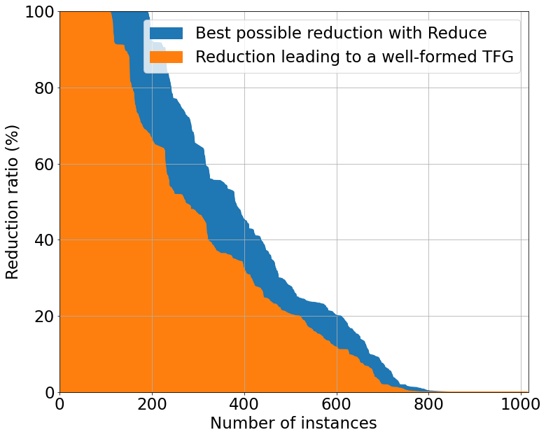
(a) All instances

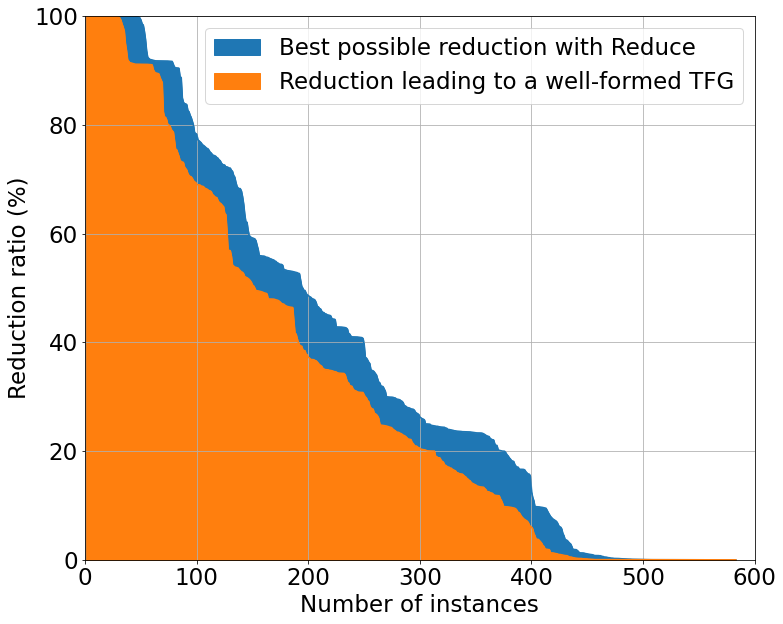
(b) Safe instances

Figure 7: Distribution of reduction ratios over: (a) all the instances in the MCC (b) all the safe instances in the MCC.

We also observe that we lose few opportunities to reduce a net due to our well-formedness constraint. Actually, we mostly lose the ability to simplify some instances of “partial” marking graphs that could be reduced using inhibitor arcs, or weights on the arcs (two features not supported by cæsar.bdd).

9.2.2 Benchmark for marking reachability

We evaluated the performance of Kong for the marking reachability problem using a selection of $426$ Petri nets taken from instances with a reduction ratio greater than $1\%$. To avoid any bias introduced by models with a large number of instances, we selected at most $5$ instances with a similar reduction ratio from each model. For each instance, we generated $5$ queries that are markings found using a “random walk” on the state space of the net (for this, we used the tool Walk that is part of the Tina distribution). We ran Kong  and Sift on each of those queries with a time limit of $5\text{\,}\mathrm{min}$.

9.2.3 Benchmark for concurrency relation

We evaluated the performance of Kong on the $424$ instances of safe Petri nets with a reduction ratio greater than $1\%$. We ran Kong  and cæsar.bdd on each of those instances, in two main modes: first with a time limit of $15\text{\,}\mathrm{min}$ to compare the number of totally solved instances (when the tool compute a complete concurrency matrix); next with a timeout of $60\text{\,}\mathrm{s}$ to compare the number of values (the filling ratios) computed in the partial matrices. Computation of a partial concurrency matrix with cæsar.bdd is done in two phases: first a “BDD exploration” phase that can be stopped by the user; then a post-processing phase that cannot be stopped. In practice this means that the execution time on the initial net is often longer than with the reduced one: the mean computation time for cæsar.bdd is about $48\text{\,}\mathrm{s}$ and less than $12\text{\,}\mathrm{s}$ for Kong. In each test, we compared the output of Kong  with the values obtained on the initial net with cæsar.bdd, and achieved $100\%$ reliability.

Next, we give details about the results obtained with our experiments and analyze the impact of using reductions.

9.3 Results on marking reachability

We display our results in the charts of Fig. 8, which compare the time needed to compute a given number of queries, with and without using reductions. (Note that we use a logarithmic scale for the time value). We consider two different samples of instances. First only the instances with a high reduction ratio (in the interval $[0.5,1]$), then the complete set of instances.

We observe a clear advantage when we use reductions. For instance, with instances that have a reduction ratio in the interval $[0.5,1]$, and with a time limit of $5\text{\,}\mathrm{min}$, we almost double the number of computed queries (from $181$ with Sift alone, versus $357$ with Kong). On the opposite, the small advantage of Sift alone, when the running time is below $0.1\text{\,}\mathrm{s}$, can be explained by the fact that we integrate the running time of Reduce to the one of Kong.

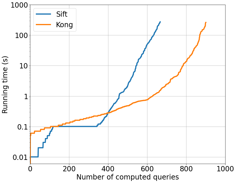
(a) $r\in]0,1]$

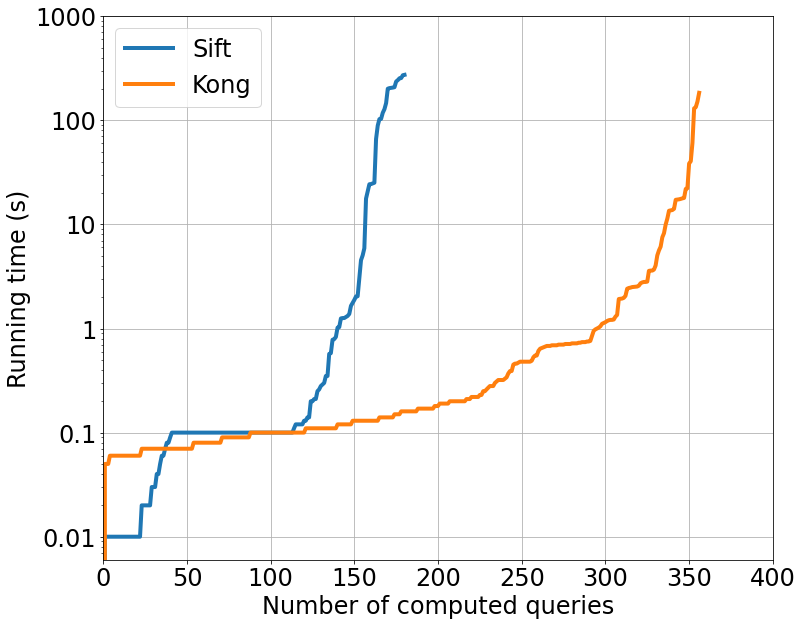
(b) $r\in[0.5,1]$

Figure 8: Minimal running time to compute a given number of reachability queries for: (a) all instances, (b) instances with $r\in[0.5,1]$.

9.4 Totally computed concurrency matrices

Our next results are for the computation of complete matrices, with a timeout of $15\text{\,}\mathrm{min}$. We give the number of computed instances in the table below. We split the results along three different categories of instances, Low/Fair/High, associated with different ratio ranges. We observe that we can compute more results with reductions than without ($+30\%$). As could be expected, the gain is greater on category High ($+86\%$), but it is still significant with the Fair instances ($+28\%$).

Reduction Ratio ($r$)			# Test Cases		# Computed Matrices
					Kong		cæsar.bdd
Low	$r\in\;]0,0.25[$		$160$		${85}$		${87}$		$\times$trunc(85 / 87, 2)
Fair	$r\in\;[0.25,0.5[$		$112$		${49}$		${38}$		$\times$trunc(49 / 38, 2)
High	$r\in\;[0.5,1]$		$152$		${95}$		${51}$		$\times$trunc(95 / 51, 2)
Total	$r\in\;]0,1]$		$\fpeval{160+112+152}$		${\fpeval{85+49+95}}$		${\fpeval{87+38+51}}$		$\times$trunc(85 + 49 + 95 / 87 + 38 + 51, 2)

Like in the previous case, we study the speed-up obtained with Kong using charts that compare the time needed to compute a given number of instances; see Fig. 9.

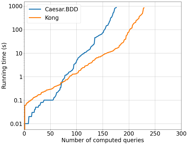
(a) $r\in]0,1]$

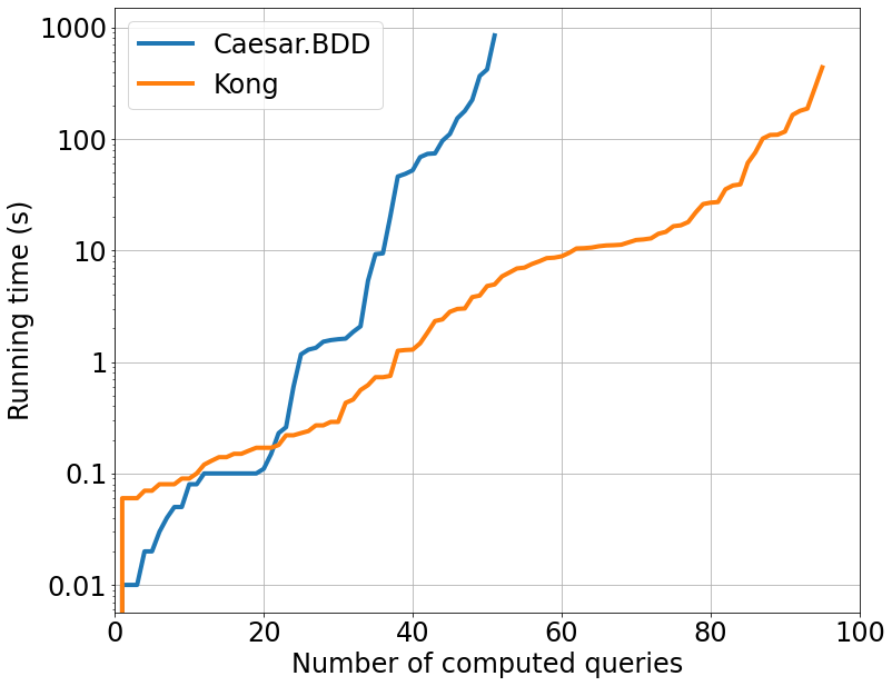
(b) $r\in[0.5,1]$

Figure 9: Minimal running time to compute a given number of concurrency matrices for: (a) all instances, (b) instances with $r\in[0.5,1]$.

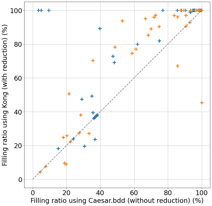
Figure 10: Comparing the filling ratio for partial matrices with Kong ($y$-axis) and cæsar.bdd ($x$-axis) for instances with $r\in[0.25,0.5[$ (light orange) and $r\in[0.5,1]$ (dark blue). (Computations done with a BDD exploration timeout of $60\text{\,}\mathrm{s}$.)

9.5 Results with partial matrices

We can also compare the “accuracy” of our approach when we have incomplete results. To this end, we compute the concurrency relation with a timeout of $60\text{\,}\mathrm{s}$ on cæsar.bdd. We compare the filling ratio obtained with and without reductions. For a net with $n$ places, this ratio is given by the formula ${2\,\mbox{{}\rm\sf\leavevmode\hbox{}\hbox{}$\mathrm{C}$\/}}/{(n^{2}+n)}$,where$\mbox{{}\rm\sf\leavevmode\hbox{}\hbox{}$\mathrm{C}$\/}$isthenumberof$0$sand$1$sinthematrix.\par Wedisplayourresultsusingascatterplotwithlinearscale,seeFig.~{}\ref{fig:partial_computations}.Weobservethatalmostallthedatapointsareononesideofthediagonal,meaninginthiscasethatreductionsincreasethenumberofcomputedvalues,withmanyexamples(toplineoftheplot)wherewecancomputethecompleterelationin$$60\text{\,}\mathrm{s}$$onlyusingreductions.Thegraphicdoesnotdiscriminatebetweenthenumberof$1$sand$0$s,butweobtainsimilargoodresultswhenweconsiderthefillingratioforonlytheconcurrentplaces(the$1$s)oronlythenonconcurrentplaces(the$0$s).\par\par\par\par\@@numbered@section{section}{toc}{Conclusion and further work} \par We propose a new method to transpose the computation of reachability problems from an initial ``high-dimensionality'' domain (the set of places in the initial net) into a smaller one (the set of places in the reduced net). Our approach is based on a combination of structural reductions with linear equations first proposed in~{}\cite[cite]{[\@@bibref{}{berthomieu2018petri,berthomieu_counting_2019}{}{}]}. \par Our main contribution, in the current work, is the definition of a new data-structure that precisely captures the structure of these linear equations, what we call the Token Flow Graph (TFG). We show how to use the TFGs to accelerate the marking reachability problem, and also for computing the concurrency relation, both in the complete and partial cases. \par We have several ideas on how to apply TFGs to other problems and how to extend them. A natural application would be for model counting (our original goal in~{}\cite[cite]{[\@@bibref{}{berthomieu2018petri}{}{}]}), where the TFG could lead to new algorithms for counting the number of (integer) solutions in the systems of linear equations that we manage. \par Another possible application is the \emph{max-marking} problem, which means finding the maximum of the expression $\sum_{p\in P}m(p)$ over all reachable markings. On safe nets, this amounts to finding the maximal number of places that can be marked together. We can easily adapt our algorithm to compute this value and could even adapt it to compute the result when the net is not safe. \par We can even manage a more general problem, related to the notion of \emph{max-concurrent} sets of places. We say that the set $S$ is concurrent if there is a reachable $m$ such that $m(p)>0$ for all places $p$ in $S$. (This subsumes the case of pairs and singleton of places.) The set $S$ is \emph{max-concurrent} if no superset $S^{\prime}\supsetneq S$ is concurrent. \par Computing the max-concurrent sets of a net is interesting for several reasons. First, it gives an alternative representation of the concurrency relation that can sometimes be more space efficient: (1) the max-concurrent sets provide a unique cover of the set of places of a net, and (2) we have $p\mathbin{\|}q$ if and only if there is $S$ max-concurrent such that $\{p,q\}\subset S$. Obviously, on safe nets, the size of the biggest max-concurrent set is the answer to the \emph{max-marking} problem. \par For future work, we would like to answer even more difficult questions, such as proofs of Generalized Mutual Exclusion Constraints~{}\cite[cite]{[\@@bibref{}{giua1992generalized}{}{}]}, that requires checking invariants involving weighted sums over the marking of places, of the form $\sum_{p\in P}w_{p}.m(p)$. Another possible extension will be to support non-ordinary nets (which would require adding weights on the arcs of the TFG) and nets that are not safe (which can already be done with our current approach, but require changing some ``axioms'' used in our algorithm).\\ \par\noindent{Acknowledgements.} We would like to thank Pierre Bouvier and Hubert Garavel for their insightful suggestions that helped improve the quality of this paper. \par\par\bibstyle{plain} \thebibliography\lx@bibitem{tacas} Nicolas Amat, Bernard Berthomieu, and Silvano Dal~{}Zilio. \lx@bibnewblock On the combination of polyhedral abstraction and {SMT}-based model checking for {Petri} nets. \lx@bibnewblock In {\em Application and Theory of Petri Nets and Concurrency (Petri Nets)}, volume 12734 of {\em{LNCS}}. Springer, 2021. \par\lx@bibitem{fi2022} Nicolas Amat, Bernard Berthomieu, and Silvano {Dal Zilio}. \lx@bibnewblock A polyhedral abstraction for {Petri} nets and its application to {SMT}-based model checking. \lx@bibnewblock{\em Fundamenta Informaticae}, 187(2-4), 2022. \par\lx@bibitem{spin2021} Nicolas Amat, Silvano Dal~{}Zilio, and Didier Le~{}Botlan. \lx@bibnewblock Accelerating the computation of dead and concurrent places using reductions. \lx@bibnewblock In {\em Model Checking Software {(SPIN)}}, volume 12864 of {\em{LNCS}}. Springer, 2021. \par\lx@bibitem{mcc2019} Elvio Amparore, Bernard Berthomieu, Gianfranco Ciardo, Silvano Dal~{}Zilio, Francesco Gall{\`{a}}, Lom~{}Messan Hillah, Francis Hulin-Hubard, Peter~{}Gj{\o}l Jensen, Lo{\"{i}}g Jezequel, Fabrice Kordon, Didier Le~{}Botlan, Torsten Liebke, Jeroen Meijer, Andrew Miner, Emmanuel Paviot-Adet, Ji{\v{r}}{\'{i}} Srba, Yann Thierry-Mieg, Tom van Dijk, and Karsten Wolf. \lx@bibnewblock Presentation of the 9th edition of the {Model Checking Contest}. \lx@bibnewblock In {\em Tools and Algorithms for the Construction and Analysis of Systems ({TACAS})}, volume 11429 of {\em{LNCS}}. Springer, 2019. \par\lx@bibitem{berthelot_transformations_1987} G.~{}Berthelot. \lx@bibnewblock Transformations and {Decompositions} of {Nets}. \lx@bibnewblock In {\em Petri Nets: Central Models and their Properties}, volume 254 of {\em{LNCS}}. Springer, 1987. \par\lx@bibitem{berthomieu2018petri} Bernard Berthomieu, Didier Le~{}Botlan, and Silvano Dal~{}Zilio. \lx@bibnewblock Petri net reductions for counting markings. \lx@bibnewblock In {\em Model Checking Software {(SPIN)}}, volume 10869 of {\em{LNCS}}. Springer, 2018. \par\lx@bibitem{berthomieu_counting_2019} Bernard Berthomieu, Didier Le~{}Botlan, and Silvano Dal~{}Zilio. \lx@bibnewblock Counting {Petri} net markings from reduction equations. \lx@bibnewblock{\em International Journal on Software Tools for Technology Transfer}, 2019. \par\lx@bibitem{bonneland2019stubborn} Frederik~{}M B{\o}nneland, Jakob Dyhr, Peter~{}G Jensen, Mads Johannsen, and Ji{\v{r}}{\'{\i}} Srba. \lx@bibnewblock Stubborn versus structural reductions for {Petri} nets. \lx@bibnewblock{\em Journal of Logical and Algebraic Methods in Programming}, 102, 2019. \par\lx@bibitem{pbhg2021} Pierre Bouvier and Hubert Garavel. \lx@bibnewblock Efficient algorithms for three reachability problems in safe petri nets. \lx@bibnewblock In {\em Application and Theory of Petri Nets and Concurrency (Petri Nets)}, volume 12734 of {\em{LNCS}}. Springer, 2021. \par\lx@bibitem{janicki_automatic_2020} Pierre Bouvier, Hubert Garavel, and Hern{\'{a}}n Ponce-de Le{\'{o}}n. \lx@bibnewblock Automatic decomposition of {Petri} nets into automata networks -- a synthetic account. \lx@bibnewblock In {\em Application and {Theory} of {Petri} {Nets} and {Concurrency} (Petri Nets)}, volume 12152. Springer, 2020. \par\lx@bibitem{garavel_nested-unit_2019} Hubert Garavel. \lx@bibnewblock Nested-unit {Petri} nets. \lx@bibnewblock{\em Journal of Logical and Algebraic Methods in Programming}, 104:60--85, April 2019. \par\lx@bibitem{garavel2021proposal} Hubert Garavel. \lx@bibnewblock{Proposal for Adding Useful Features to Petri-Net Model Checkers}. \lx@bibnewblock Research Report 03087421, {Inria Grenoble - Rh{\^{o}}ne-Alpes}, December 2020. \par\lx@bibitem{garavel_state_2004} Hubert Garavel and Wendelin Serwe. \lx@bibnewblock State {Space} {Reduction} for {Process} {Algebra} {Specifications}. \lx@bibnewblock In {\em Algebraic {Methodology} and {Software} {Technology}}, volume 3116 of {\em{LNCS}}. Springer, 2004. \par\lx@bibitem{giua1992generalized} Alessandro Giua, Frank DiCesare, and Manuel Silva. \lx@bibnewblock Generalized mutual exclusion contraints on nets with uncontrollable transitions. \lx@bibnewblock In {\em IEEE International Conference on Systems, Man, and Cybernetics}. IEEE, 1992. \par\lx@bibitem{HillahK17} Lom{-}Messan Hillah and Fabrice Kordon. \lx@bibnewblock{Petri Nets Repository}: A tool to benchmark and debug {Petri} net tools. \lx@bibnewblock In {\em Application and Theory of Petri Nets and Concurrency (Petri Nets)}, volume 10258 of {\em LNCS}. Springer, 2017. \par\lx@bibitem{hillah2010pnml} Lom-Messan Hillah, Fabrice Kordon, Laure Petrucci, and Nicolas Treves. \lx@bibnewblock{PNML} framework: an extendable reference implementation of the {Petri Net Markup Language}. \lx@bibnewblock In {\em International Conference on Applications and Theory of Petri Nets}, volume 6128 of {\em{LNCS}}. Springer, 2010. \par\lx@bibitem{hujsa:hal-02992521} Thomas Hujsa, Bernard Berthomieu, Silvano Dal~{}Zilio, and Didier Le~{}Botlan. \lx@bibnewblock{Checking marking reachability with the state equation in {Petri} net subclasses}. \lx@bibnewblock Technical Report 20278, LAAS-CNRS, November 2020. \par\lx@bibitem{cadp} INRIA. \lx@bibnewblock{CADP}. \lx@bibnewblock\url{https://cadp.inria.fr/}, 2020. \par\lx@bibitem{janicki_nets_1984} Ryszard Janicki. \lx@bibnewblock Nets, sequential components and concurrency relations. \lx@bibnewblock{\em Theoretical Computer Science}, 29(1-2), 1984. \par\lx@bibitem{kovalyov_concurrency_1992} A.~{}V. Kovalyov. \lx@bibnewblock Concurrency relations and the safety problem for {Petri} nets. \lx@bibnewblock In {\em Application and {Theory} of {Petri} {Nets}}, volume 616 of {\em{LNCS}}, Berlin, Heidelberg, 1992. Springer. \par\lx@bibitem{kovalyov_polynomial_2000} Andrei Kovalyov. \lx@bibnewblock A {Polynomial} {Algorithm} to {Compute} the {Concurrency} {Relation} of a {Regular} {STG}. \lx@bibnewblock In {\em Hardware {Design} and {Petri} {Nets}}. Springer, Boston, MA, 2000. \par\lx@bibitem{tinaToolbox} LAAS-CNRS. \lx@bibnewblock Tina {Toolbox}. \lx@bibnewblock\url{http://projects.laas.fr/tina}, 2020. \par\lx@bibitem{lipton_reduction_1975} Richard~{}J. Lipton. \lx@bibnewblock Reduction: a method of proving properties of parallel programs. \lx@bibnewblock{\em Communications of the ACM}, 18(12), 1975. \par\lx@bibitem{murata1989petri} Tadao Murata. \lx@bibnewblock Petri nets: Properties, analysis and applications. \lx@bibnewblock{\em Proceedings of the IEEE}, 77(4), 1989. \par\lx@bibitem{semenov_combining_1995} A.~{}Semenov and A.~{}Yakovlev. \lx@bibnewblock Combining partial orders and symbolic traversal for efficient verification of asynchronous circuits. \lx@bibnewblock In {\em Proceedings of {ASP}-{DAC}'95/{CHDL}'95/{VLSI}'95 with {EDA} {Technofair}}, 1995. \par\lx@bibitem{silva1996linear} Manuel Silva, Enrique Terue, and Jos{\'{e}}~{}Manuel Colom. \lx@bibnewblock Linear algebraic and linear programming techniques for the analysis of place/transition net systems. \lx@bibnewblock In {\em Lectures on Petri Nets I: Basic Models: Advances in Petri Nets}, volume 1491 of {\em{LNCS}}. Springer, 1996. \par\lx@bibitem{thierry-mieg_structural_2020} Yann Thierry-Mieg. \lx@bibnewblock Structural reductions revisited. \lx@bibnewblock In {\em Application and Theory of Petri Nets and Concurrency (Petri Nets)}, volume 12152 of {\em{LNCS}}. Springer, 2020. \par\lx@bibitem{wisniewski_prototyping_2018} Remigiusz Wisniewski, Andrei Karatkevich, Marian Adamski, Aniko Costa, and Luis Gomes. \lx@bibnewblock Prototyping of {Concurrent} {Control} {Systems} with {Application} of {Petri} {Nets} and {Comparability} {Graphs}. \lx@bibnewblock{\em IEEE Transactions on Control Systems Technology}, 26(2), 2018. \par\lx@bibitem{wisniewski2019c} Remigiusz Wi{\'{s}}niewski, Monika Wi{\'{s}}niewska, and Marcin Jarnut. \lx@bibnewblock{C-exact} hypergraphs in concurrency and sequentiality analyses of cyber-physical systems specified by safe {Petri} nets. \lx@bibnewblock{\em IEEE Access}, 7, 2019. \par\endthebibliography \par\@add@PDF@RDFa@triples\par\end{document}$